A Bayesian analysis of kaon photoproduction with the Regge-plus-resonance model

Abstract

We address the issue of unbiased model selection and propose a methodology based on Bayesian inference to extract physical information from kaon photoproduction $p(\gamma,K^{+})\Lambda$ data. We use the single-channel Regge-plus-resonance (RPR) framework for $p(\gamma,K^{+})\Lambda$ to illustrate the proposed strategy. The Bayesian evidence $\mathcal{Z}$ is a quantitative measure for the model’s fitness given the world’s data. We present a numerical method for performing the multidimensional integrals in the expression for the Bayesian evidence. We use the $p(\gamma,K^{+})\Lambda$ data with an invariant energy $W>2.6$ GeV in order to constrain the background contributions in the RPR framework with Bayesian inference. Next, the resonance information is extracted from the analysis of differential cross sections, single and double polarization observables. This background and resonance content constitutes the basis of a model which is coined RPR-2011. It is shown that RPR-2011 yields a comprehensive account of the kaon photoproduction data and provides reasonable predictions for $p(e,e^{\prime}K^{+})\Lambda$ observables.

I Introduction

How to extract the nucleon resonance $(N^{\ast})$ content of the open strangeness photoproduction reactions $p(\gamma,K^{+})\Lambda$ is a long-standing question. Various analyses lead to disparate outcomes concerning the set of resonances that are likely to contribute David et al. (1996); Ireland et al. (2004); Julia-Diaz et al. (2006); Mart and Bennhold (1999); Shklyar et al. (2005); Usov and Scholten (2006); Shyam et al. (2010); Maxwell (2012). The recent availability of abundant high-statistics data has not profoundly changed the situation so far. This indeterminacy for the open strangeness channel is in stark contrast to the situation for pionic channels, where the contributing resonances can be successfully identified by means of a partial wave analysis for invariant energies $W<1.8$ GeV. In open strangeness channels, this technique is less powerful as the nonresonant, or background, contributions are larger. The importance of background contributions calls for a framework which accounts for resonant and nonresonant processes and which provides a means to constrain both classes of reaction mechanisms independently.

An efficient way of pinpointing the background amplitude involves Regge phenomenology Corthals et al. (2006); Anisovich et al. (2011). We will describe the $p(\gamma,K^{+})\Lambda$ reaction in the so-called Regge-plus-resonance (RPR) model, which combines ingredients of Regge phenomenology with elements of a typical isobar approach. The latter belongs to the class of tree-level effective Lagrangian models. In the RPR framework, the background amplitude is constrained by optimizing the adjustable parameters of a Reggeized background model to data obtained at sufficiently high energies so that the contribution of individual resonances is projected to become marginal Corthals et al. (2006); Sibirtsev et al. (2007).

Even with a properly constrained background contribution, the identification of the contributing resonances to $p(\gamma,K^{+})\Lambda$ remains a precarious task. Adding resonances increases the amount of adjustable parameters and improves the quality of the fit to the data. It stands to reason that one should not add more resonances than strictly necessary, in order to obtain a good model. One of the guiding principles for model selection is Occam’s razor Rodriguez-Fernandez (1999). This principle dictates that if one has to choose between a simple and a more complex model, all else being equal, the simpler one should be preferred. In a realistic situation, however, all else is not equal, and this guiding principle should somehow be translated to a quantitative measure which balances between model complexity on the one hand and accuracy on the other hand. Such a measure can be derived from first principles using Bayesian inference. This measure, called the Bayesian evidence $\mathcal{Z}$, evaluates the overall performance of the model while penalizing for excessive complexity.

In recent years, much effort has been directed towards a more comprehensive description of both electromagnetic and hadronic meson production reactions from the nucleon within coupled-channels frameworks Julia-Diaz et al. (2006); Anisovich et al. (2011); Suzuki et al. (2010). Ideally, one would like to apply Bayesian inference to a state-of-the-art dynamical coupled-channels model. However, due to the multidimensional integrals involved in the computation of the Bayesian evidence, one is stricken by the curse of dimensionality: at worst, the computational cost increases exponentially with the number of adjustable parameters. Even if the number of adjustable parameters is kept in check, the sheer number of model evaluations required for a Monte Carlo integration calls for a realistic model of modest complexity. In this work, we will apply Bayesian inference to the single-channel RPR framework for kaon photoproduction. We will consider several variants of the RPR model and use Bayesian inference to select the most probable model given the world’s data. The RPR model has been shown to efficiently describe the $p(\gamma,K^{+})\Lambda$ observables over a broad energy range Corthals et al. (2006); Corthals et al. (2007a); Vancraeyveld et al. (2009). The RPR framework, as it will be used in this work, has a modest number of adjustable parameters. The background in the RPR framework consists of Reggeized $K^{+}(494)$ and $K^{\ast+}(892)$ exchange in the $t$ channel. With these assumptions, the background part has two unknown phases and three unknown coupling constants. In addition to the background, the RPR model incorporates $N^{\ast}$ in the $s$ channel. The improved version of the RPR model, as it will be introduced in this work, uses consistent $N^{*}$ interaction Lagrangians and this is an enormous asset in order to reduce the number of coupling strengths Vrancx et al. (2011). For each added $N^{\ast}$ one introduces one unknown coupling constant for $J=\frac{1}{2}$ and two unknown coupling constants for $J\geq\frac{3}{2}$.

The outline of the remainder of this paper is as follows. In Section II.1 the observables and kinematics of the $N(\gamma,K)Y$ and $N(e,e^{\prime}K)Y$ reactions are introduced. In Section  II.2 we summarize the underlying assumptions of the Regge-plus-resonance formalism used to describe these reactions. Section III discusses a Bayesian approach to model selection. The computation of the Bayesian evidence is a high-dimensional problem which requires dedicated numerical methods and strategies. In Section III.4 we provide details of these methods. A proof of principle of the adopted numerical strategy is described in Section III.5. Bayesian methodology is applied to determine the Reggeized background amplitude in Section IV. In Section V, we determine the optimal resonant content for $p(\gamma,K^{+})\Lambda$ by evaluating a set of 11 candidate resonances. For each of them we compute the relative resonance probability and the results are presented in Section V.3. The results for the various photoproduction observables and predictions for electroproduction observables are presented in Sections V.4 and V.5. A conclusion is given in Section VI.

II Regge-plus-resonance formalism

II.1 Observables and kinematics

II.1.1 Photoproduction

The unpolarized cross section for $N(\gamma,K)Y$ has the following expression

$$d\sigma =\int\frac{1}{\nu_{rel}(2\omega)(2E_{N})}\frac{d^{3}\bm{p}_{K}}{\left(2\pi\right)^{3}}\frac{1}{2E_{K}}\frac{d^{3}\bm{p}_{Y}}{\left(2\pi\right)^{3}}\frac{1}{2E_{Y}}\left(2\pi\right)^{4}$$

$$\times \delta^{\left(4\right)}\left(p_{N}+k-p_{K}-p_{Y}\right)\frac{1}{4}\sum_{{\lambda_{\gamma}},\lambda_{N},\lambda_{Y}}\left|\mathcal{M}^{\lambda_{N}\lambda_{Y}}_{\lambda_{\gamma}}\right|^{2},$$ (1)

where $\nu_{rel}$ is the relative photon-nucleon energy, the $p_{N}(E_{N},\vec{p}_{N})$, $k(\omega,\vec{k})$, $p_{K}(E_{K},\vec{p}_{K})$, and $p_{Y}(E_{Y},\vec{p}_{Y})$ are the four-momenta of the nucleon, photon, kaon, and hyperon. The $\lambda_{\gamma}$, $\lambda_{N}$ and $\lambda_{Y}$ denote the photon, nucleon, and hyperon polarization.

In the center-of-momentum (c.m.) frame, the particles’ four-momenta are defined as follows:

$$k^{\ast} =(\omega^{\ast},\bm{k^{\ast}}) p_{K}^{\ast} =(E^{\ast}_{K},\bm{p}^{\ast}_{K})$$

$$p_{N}^{\ast} =(E^{\ast}_{N},-\bm{k}^{\ast}) p_{Y}^{\ast} =(E^{\ast}_{Y},\bm{p}^{\ast}_{Y})=(E^{\ast}_{Y},-\bm{p}^{\ast}_{K}).$$ (2)

The $\bm{z}$-axis is the propagation direction of the incident photon, and the $\bm{xz}$-plane is the reaction plane.

Inserting the c.m. momenta of Eq. (2) into Eq. (1) yields the expression for the unpolarized differential cross section at fixed $\left(s=W^{2}=\left(k^{\ast}+p_{N}^{\ast}\right)^{2},t=\left(p_{K}^{\ast}-k^{\ast}\right)^{2}\right)$

$$\frac{d\sigma}{d\Omega^{\ast}_{K}}= \,\frac{1}{64\pi^{2}}\frac{\left|\bm{p}^{\ast}_{K}\right|}{\omega^{\ast}}\frac{1}{\left(E_{N}^{\ast}+\omega^{\ast}\right)^{2}}$$

$$\times \frac{1}{4}\sum_{{\lambda_{\gamma}},\lambda_{N},\lambda_{Y}}\left|\mathcal{M}^{\lambda_{N}\lambda_{Y}}_{\lambda_{\gamma}}\right|^{2},$$ (3)

where the transition amplitude can be written as the product of the photon polarization vector $\varepsilon^{\mu}_{{\lambda_{\gamma}}}$ and the hadronic current $\mathcal{M}^{\lambda_{N}\lambda_{Y}}_{\lambda_{\gamma}}=\varepsilon^{\mu}_{{\lambda_{\gamma}}}J^{\lambda_{N}\lambda_{Y}}_{\mu}$. The hadronic current adopts the form

$$J^{\lambda_{N}\lambda_{Y}}_{\mu} =\,\overline{u}_{\lambda_{Y}}^{Y}(p_{Y})\;T_{\mu}\;\,u_{\lambda_{N}}^{N}(p_{N})\;,$$ (4)

where $\,u_{\lambda_{Y}}^{Y}(p_{Y})$ and $\,u_{\lambda_{N}}^{N}(p_{N})$ are the hyperon and nucleon spinors.

The target ($T$) and recoil ($P$) asymmetries are defined as

$$T,P=\frac{d\sigma^{\lambda_{X}=+\frac{1}{2}}-d\sigma^{\lambda_{X}=-\frac{1}{2}}}{d\sigma^{\lambda_{X}=+\frac{1}{2}}+d\sigma^{\lambda_{X}=-\frac{1}{2}}},$$ (5)

where $d\sigma\equiv\frac{d\sigma}{d\Omega_{K}^{\ast}}$, and $\lambda_{X}$ is the nucleon and hyperon spin projection on the $\bm{y}$-axis, respectively. The beam asymmetry $\Sigma$ follows the definition

$$\Sigma=\frac{d\sigma^{\perp}-d\sigma^{\parallel}}{2d\sigma},$$ (6)

where $\sigma^{\perp}$($\sigma^{\parallel}$) refers to a linear photon polarization along the $\bm{y}$($\bm{x}$) axis.

Double polarization observables are defined as

$$\frac{d\sigma^{(++)}+d\sigma^{(--)}-d\sigma^{(+-)}-d\sigma^{(-+)}}{d\sigma^{(++)}+d\sigma^{(--)}+d\sigma^{(+-)}+d\sigma^{(-+)}},$$ (7)

where $(+-)$ is a shorthand notation for $(\lambda_{A}=+s_{A},\lambda_{B}=-s_{B})$, the polarizations of the particles $A$ and $B$ that determine the asymmetry. Beam-recoil $p(\gamma,K^{+})\Lambda$ double polarization data are available for circularly $(C_{x},C_{z})$ and obliquely $(O_{x},O_{z})$ polarized photon beams. These are more commonly expressed in the “primed” reference frame, which is rotated about the $\bm{y}=\bm{y}^{\prime}$-axis over an angle $\theta_{K}^{\ast}$, with $\theta_{K}^{\ast}$ the angle between the incoming photon and the outgoing kaon momentum in the c.m. frame.

II.1.2 Electroproduction

For incoming and outgoing electron four-momenta $k_{1}(\epsilon_{1},\vec{k}_{1})$ and $k_{2}(\epsilon_{2},\vec{k}_{2})$ the electroproduction cross section in the one-photon exchange approximation (OPEA) has the following form

$$d\sigma= \int\frac{1}{\nu_{{rel}}2\epsilon_{1}2E_{N}}\frac{d^{3}\bm{p}_{Y}}{\left(2\pi\right)^{3}}\frac{1}{2E_{Y}}\frac{d^{3}\bm{k}_{2}}{\left(2\pi\right)^{3}}\frac{1}{2\epsilon_{2}}\frac{d^{3}\bm{p}_{K}}{\left(2\pi\right)^{3}}\frac{1}{2E_{K}}$$

$$\times\left(2\pi\right)^{4}\delta^{(4)}\left(p_{N}+k_{1}-p_{K}-p_{Y}-k_{2}\right)\frac{1}{4}\sum_{\lambda_{i}}\left|\mathcal{T}_{\lambda_{i}}\right|^{2},$$ (8)

where the hadronic part of the reaction is evaluated in the $\gamma^{\ast}N$ c.m. frame and the leptonic part in the laboratory frame $\left(p_{N}^{\text{lab}}\equiv(m_{N},\bm{0})\right)$. This yields the following expression for the unpolarized differential cross section

$$\frac{d^{3}\sigma}{d\epsilon_{2}^{\text{lab}}d\Omega_{2}^{\text{lab}}d\Omega^{\ast}_{K}}= \frac{1}{32(2\pi)^{5}}\frac{1}{m_{N}}\frac{\left|\bm{p}^{\ast}_{K}\right|}{W}\frac{\epsilon_{2}^{\text{lab}}}{\epsilon_{1}^{\text{lab}}}$$

$$\times \frac{1}{4}\sum_{\lambda_{1}\lambda_{2}\lambda_{N}\lambda_{Y}}{\left|\mathcal{T}^{\lambda_{1}\lambda_{2}}_{\lambda_{N}\lambda_{Y}}\right|^{2}},$$ (9)

where $\epsilon_{1}^{\text{lab}}$ ($\epsilon_{2}^{\text{lab}}$) is the incoming (outgoing) electron energy in the lab frame and $W$ is the invariant energy.

In the transition amplitude $\mathcal{T}^{\lambda_{1}\lambda_{2}}_{\lambda_{N}\lambda_{Y}}$, $\lambda_{1}$ and $\lambda_{2}$ are the polarizations (for high-energy electrons equal to the helicities) of the incoming and outgoing electron. This amplitude has a leptonic and a hadronic current, connected by a photon propagator

$$\mathcal{T}^{\lambda_{1}\lambda_{2}}_{\lambda_{N}\lambda_{Y}}=e\;l_{\mu}^{\lambda_{1}\lambda_{2}}\;\left(\frac{-g^{\mu\nu}}{k^{2}}\right)\;J^{\lambda_{N}\lambda_{Y}}_{\nu},$$ (10)

where the hadronic current $J^{\lambda_{N}\lambda_{Y}}_{\nu}$ is defined in Eq. (4), $l_{\mu}^{\lambda_{1}\lambda_{2}}$ is the leptonic current, and $k^{2}=(k_{2}-k_{1})^{2}=-Q^{2}$.

Therefore, $\mathcal{T}^{\lambda_{1}\lambda_{2}}_{\lambda_{N}\lambda_{Y}}$ can be linked to $\mathcal{M}_{\lambda_{\gamma}}^{\lambda_{N}\lambda_{Y}}$ and one can write

$$\mathcal{T}^{\lambda_{1}\lambda_{2}}_{\lambda_{N}\lambda_{Y}}=\frac{e}{Q^{2}}\sum_{{\lambda_{\gamma}}=-1,0,+1}{(-1)^{\lambda_{\gamma}}L_{\lambda_{\gamma}}^{\lambda_{1}\lambda_{2}\ast}\mathcal{M}_{\lambda_{\gamma}}^{\lambda_{N}\lambda_{Y}}},$$ (11)

where the photon propagator was rewritten using the relation

$$\sum_{{\lambda_{\gamma}}=0,\pm 1}{\left(-1\right)^{\lambda_{\gamma}}\varepsilon^{\ast\mu}_{{\lambda_{\gamma}}}\varepsilon^{\nu}_{{\lambda_{\gamma}}}}=g^{\mu\nu}+\frac{k^{\mu}k^{\nu}}{Q^{2}},$$ (12)

and $Q^{2}=-k^{2}$ is the photon virtuality.

The tensor $L_{{\lambda_{\gamma}}}^{\lambda_{1}\lambda_{2}}$ is defined as a contraction between the photon polarization four-vector and the leptonic current

$$L_{{\lambda_{\gamma}}}^{\lambda_{1}\lambda_{2}\ast}=l^{\lambda_{1}\lambda_{2}}_{\mu}\varepsilon^{\ast\mu}_{\lambda_{\gamma}}.$$ (13)

Using Eq. (11) in the OPEA, one can conveniently separate the quantum electrodynamics (QED) part from the hadronic part, by defining the two tensors

$$\mathcal{L}_{{\lambda_{\gamma}}{\lambda_{\gamma}}^{\prime}} =\sum_{\lambda_{1},\lambda_{2}}(-1)^{{\lambda_{\gamma}}+{\lambda_{\gamma}}^{\prime}}L_{{\lambda_{\gamma}}}^{\lambda_{1}\lambda_{2}}\left(L_{{\lambda_{\gamma}}}^{\lambda_{1}\lambda_{2}}\right)^{\dagger}\;,$$ (14)

$$\mathcal{H}_{{\lambda_{\gamma}}{\lambda_{\gamma}}^{\prime}} =\sum_{\lambda_{N},\lambda_{Y}}\mathcal{M}_{\lambda_{\gamma}}^{\lambda_{N}\lambda_{Y}}\left(\mathcal{M}_{{\lambda_{\gamma}}^{\prime}}^{\lambda_{N}\lambda_{Y}}\right)^{\dagger}.$$ (15)

This allows one to replace the squared transition amplitude in Eq. (9) by

$$\sum_{\lambda_{1},\lambda_{2},\lambda_{N},\lambda_{Y}}\left|\mathcal{T}^{\lambda_{1}\lambda_{2}}_{\lambda_{N}\lambda_{Y}}\right|^{2}=\frac{e^{2}}{Q^{4}}\sum_{{\lambda_{\gamma}},{\lambda_{\gamma}}^{\prime}=0,\pm 1}\mathcal{L}_{{\lambda_{\gamma}}{\lambda_{\gamma}}^{\prime}}\mathcal{H}_{{\lambda_{\gamma}}{\lambda_{\gamma}}^{\prime}}.$$ (16)

After this replacement, the separated cross sections or structure functions emerge. They do not depend on the kaon azimuthal angle $\phi^{\ast}_{K}$ and are defined as

$$\dfrac{d\sigma_{T}}{d\Omega^{\ast}_{K}} =\chi\left(\mathcal{H}_{1,1}+\mathcal{H}_{-1,-1}\right)\;,$$ (17)

$$\dfrac{d\sigma_{L}}{d\Omega^{\ast}_{K}} =2\chi\mathcal{H}_{0,0}\;,$$ (18)

$$\dfrac{d\sigma_{TT}}{d\Omega^{\ast}_{K}} =-\chi\left(\mathcal{H}_{1,-1}+\mathcal{H}_{-1,1}\right)\;,$$ (19)

$$\dfrac{d\sigma_{LT}}{d\Omega^{\ast}_{K}} =-\chi\left(\mathcal{H}_{0,1}+\mathcal{H}_{1,0}-\mathcal{H}_{-1,0}-\mathcal{H}_{0,-1}\right)\;,$$ (20)

where $\chi=\frac{1}{\left(16\pi\right)^{2}Wm_{N}}\frac{\left|\bm{p}_{K}^{\ast}\right|}{\left(\omega^{\text{lab}}-\frac{Q^{2}}{2m_{N}}\right)}$.

Expressing Eq. (9) in terms of the separated cross sections, we obtain

$$\frac{d^{3}\sigma}{d\epsilon_{2}^{\text{lab}}d\Omega_{2}^{\text{lab}}d\Omega^{\ast}_{K}}= \,\Gamma\left(\dfrac{d\sigma_{T}}{d\Omega^{\ast}_{K}}+\varepsilon\dfrac{d\sigma_{L}}{d\Omega^{\ast}_{K}}+\varepsilon\dfrac{d\sigma_{TT}}{d\Omega^{\ast}_{K}}\cos{(2\phi^{\ast}_{K})}\right.$$

$$+ \left.\sqrt{\varepsilon(1+\varepsilon)}\dfrac{d\sigma_{LT}}{d\Omega^{\ast}_{K}}\cos{(\phi^{\ast}_{K})}\right),$$ (21)

in which the dependence on $\phi^{\ast}_{K}$ has been made explicit. The virtual photon flux

$$\Gamma= \frac{\alpha}{2\pi^{2}}\frac{\epsilon_{2}^{\text{lab}}}{\epsilon_{1}^{\text{lab}}}\frac{\left(\omega_{\text{lab}}-\frac{Q^{2}}{2m_{N}}\right)}{Q^{2}}\frac{1}{1-\varepsilon},$$ (22)

and the virtual photon (transverse) polarization

$$\varepsilon= \left(1+\frac{2\left|\bm{k}_{\text{lab}}\right|^{2}}{Q^{2}}\tan^{2}\frac{\theta_{e}}{2}\right)^{-1},$$ (23)

are defined in terms of the electron scattering angle $\theta_{e}$ and the virtual photon three-momentum in the lab frame $\bm{k}_{\text{lab}}$.

II.2 Regge-plus-resonance formalism

This section deals with the dynamics of kaon production as described by the Regge-plus-resonance (RPR) framework introduced in Refs. Corthals (2006); Corthals et al. (2006); Corthals et al. (2007b, a). The RPR model conjoins the economic description of high-energy data by means of Regge phenomenology with a single-channel hadrodynamical approach in the resonance region. We have stressed the importance of the background diagrams in $KY$ photoproduction for a correct determination of the resonance parameters. In a isobar model, in which the amplitude is described as a sum of tree-level $s$, $t$ and $u$-channel diagrams David et al. (1996); Janssen et al. (2002), the determination of the background is highly model dependent Janssen (2001). Another issue with isobar models is there violation of the Froissart bound Donnachie et al. (2002); Froissart (1961, 2010). Indeed, the background amplitude of isobar models displays a power-law $s^{\alpha}$ dependence at large energies where the exponent $\alpha$ depends linearly on the spin of the exchanged particles Donnachie et al. (2002). The RPR approach overcomes these shortcomings by describing the nonresonant contributions to the total amplitude by means of Regge theory Corthals et al. (2006).

II.2.1 Regge background

Guidal, Laget and Vanderhaeghen showed that the exchange of a limited number of Regge trajectories in the $t$-channel reproduces the high-energy, forward-angle data of both photoproduction Guidal et al. (1997) and electroproduction Vanderhaeghen et al. (1998); Guidal et al. (2003); Guidal (1997) of pions and kaons off the nucleon. Along those lines, the RPR background is obtained by Reggeizing the first materializations of the lightest kaon trajectories, $K^{+}(494)$ and $K^{\ast+}(892)$. The Reggeized amplitudes are obtained by replacing the $t$-channel Feynman propagator by a Regge one with the appropriate signature.

The odd-spin and even-spin kaon trajectories are observed to coincide. The measured $t$-dependence of the $d\sigma/d\Omega_{K}^{\ast}$ at large $s$ does not display any pronounced structure, and this gives additional support to the strong degeneracy of the trajectories. Therefore, the Regge propagator reduces to

$$\mathcal{P}^{K}_{\text{Regge}}(s,t)=\left(\dfrac{s}{s_{0}}\right)^{\alpha_{K}(t)}\dfrac{\pi\alpha_{K}^{\prime}}{\sin\left(\pi\alpha_{K}(t)\right)}\begin{Bmatrix}1\\ e^{-i\pi\alpha_{K}(t)}\end{Bmatrix}\\ \times\dfrac{1}{\Gamma\left(1+\alpha_{K}(t)\right)}\;,$$ (24)

where $\alpha_{K}^{\prime}$ is the slope of the trajectory and the scale factor $s_{0}$ is fixed at $1\;\mathrm{GeV}^{2}$.

The relative sign between the odd-spin and even-spin propagators determines the phase ($1$ or $e^{-i\pi\alpha_{K}(t)}$) of $\mathcal{P}^{K}_{\text{Regge}}$ and cannot be determined from first principles. The issue of determining this phase by comparing model predictions with data will be addressed in Section IV.

For vector mesons, we obtain the proper pole positions by subtracting the spin from the trajectories in the Regge propagator. For the $K^{\ast+}(892)$, the resulting propagator is

$$\mathcal{P}^{K^{\ast}}_{\text{Regge}}(s,t)=\left(\dfrac{s}{s_{0}}\right)^{\alpha_{K^{\ast}}(t)-\alpha_{0}}\dfrac{\pi\alpha_{K^{\ast}}^{\prime}}{\sin\left(\pi(\alpha_{K^{\ast}}(t)-\alpha_{0})\right)}\\ \times\begin{Bmatrix}1\\ e^{-i\pi(\alpha_{K^{\ast}}(t)-\alpha_{0})}\end{Bmatrix}\dfrac{1}{\Gamma\left(1+\alpha(t)_{K^{\ast}}-\alpha_{0}\right)}\;,$$ (25)

where $\alpha_{0}=1$. The employed parametrization for the $K^{+}(494)$ and $K^{\ast+}(892)$ trajectories is given by Janssen (2001)

$$\alpha_{K}(t) =0.70\;\mathrm{GeV}^{-2}\left(t-m_{K}^{2}\right),$$ (26)

$$\alpha_{K^{*}}(t) =1+0.85\;\mathrm{GeV}^{-2}\left(t-m_{K^{*}}^{2}\right)\;.$$ (27)

II.2.2 Gauge restoration

The $K^{+}(494)$ exchange diagram in the $t$-channel breaks gauge invariance. One way of restoring it is to add the electric part of the $s$-channel Born-diagram with the same coupling constant as in the $K^{+}$ exchange diagram. This procedure is also applicable for a Reggeized $t$-channel. It turns out to be essential for a proper description of the forward-angle differential cross sections and of the beam asymmetries in charged pion photoproduction Guidal et al. (1997).

For $p(\gamma,K^{+})\Lambda$, the gauge-restoring $s$-channel contribution is pivotal to account for the plateau in the differential cross sections at very forward kaon angles or small $|t|$ Guidal et al. (1997). The differential cross section for $p(\gamma,K^{+})\Lambda$ is shown in Fig. 1.

Along similar lines, gauge invariance for electroproduction can be restored by adopting the same $Q^{2}$-dependence in both the electromagnetic coupling of the $K^{+}$ exchange diagram and the electric part of the $s$-channel Born term. In practice, this implies that a monopole kaon form factor is assigned to the electric part of the proton exchange diagram Guidal et al. (2000). This procedure has been shown to result in a reasonable prediction of the $\sigma_{L}/\sigma_{T}$ ratio Guidal et al. (2003).

II.2.3 Adding resonance contributions

While Regge theory provides a fair description of meson photoproduction observables at high energies and forward angles, there are arguments that it can also be applied in the resonance region. Indeed, the notion of reggeon-resonance duality states that the amplitude should be reproduced by summing over all diagrams of a certain channel, be it the $s$, $u$ or $t$-channel Dolen et al. (1968).

Even though the smooth $s$ dependence of the Regge amplitude does not allow one to describe the structures in the resonance region, the global trends can be fairly reproduced Guidal et al. (2003). Furthermore, the forward peaking of the differential cross sections supports large contributions from the nonresonant $t$-channel background.

Inspired by these observations, Corthals et al. Corthals et al. (2006); Corthals et al. (2007b, a); Corthals (2006) developed a hybrid model for $KY$ photoproduction dubbed Regge-plus-resonance (RPR). We will refer to this model as RPR-2007. The RPR-2007 model uses amplitudes which consist of $s$-channel resonances and Reggeized $t$-channel background terms. This approach has also been successfully applied to the electromagnetic production of $\pi\pi$ Holvoet (2002), as well as $\eta$ and $\eta^{\prime}$ Chiang et al. (2003).

The Regge background amplitude of RPR-2007 is constrained to above-resonance ($\sqrt{s}>3$ GeV), forward-angle ($\cos{\theta_{K}^{\ast}}>0.35$) data. By extrapolating the resulting amplitude to smaller $\sqrt{s}$, one gets a parameter-free background for the resonance region. The $s$-channel resonances are coherently added to the background amplitude, resulting in a hybrid amplitude for the resonance and high-$s$ region. RPR-2007 describes the data for forward-angle photo- and electroproduction of $K^{+}\Lambda$ and $K^{+}\Sigma^{0}$ Corthals et al. (2006); Corthals et al. (2007b, a). With regard to the $N^{\ast}$’s, it includes the established PDG resonances S${}_{11}(1650)$, P${}_{11}(1710)$, P${}_{13}(1720)$, the less established P${}_{13}(1900)$, as well as the missing D${}_{13}(1900)$. The resonance parameters of the RPR-2007 model are constrained to the $\cos{\theta_{K}^{\ast}}>0.35$ data.

Figure 1: (color online). The $p(\gamma,K^{+})\Lambda$ differential cross section as a function of $\cos{\theta_{K}^{\ast}}$ for the laboratory photon-energy bins $\omega_{\text{lab}}=1575$ MeV, 1875 MeV and 2175 MeV. The line denotes the RPR-2007 result and the data are from references Glander et al. (2004); Hicks et al. (2007); Bradford et al. (2006); McCracken et al. (2010). The RPR-2007 model is optimized against the $\cos{\theta_{K}^{\ast}}>0.35$ data (indicated with the arrow).

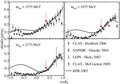
In Fig. 1 we confront the predictions of the RPR-2007 model with a selection of differential cross-section data. At forward angles the data are nicely described, in stark contrast to the situation at backward kaon angles. This failure of the model at backward angles can be largely attributed to the adopted description for the spin-3/2 resonance diagrams in RPR-2007 Vrancx et al. (2011). Obviously, unphysical bumps at backward angles manifest themselves and the situation worsens with increasing lab photon energy $\omega_{lab}$. In the forthcoming Section it is pointed out how the introduction of consistent high-spin interactions can remedy this situation.

II.2.4 Consistent high-spin interactions

In the RPR-2007 framework, spin-3/2 resonances are described by the Rarita-Schwinger formalism Rarita and Schwinger (1941). Rarita-Schwinger fields, however, contain lower-spin components, which are not physical. In the noninteracting Rarita-Schwinger theory these unphysical components are eliminated by imposing the so-called “Rarita-Schwinger constraints”. These constraints, however, do not prevent the unphysical components from participating in the interacting theory. The spurious lower-spin components generate non-localities, violate causality Velo and Zwanziger (1969), and must therefore be avoided.

The spin-3/2 interaction Lagrangians that are used in the RPR-2007 model are inconsistent since they allow for the propagation of the unphysical spin-1/2 modes of the Rarita-Schwinger field. These Lagrangians involve the coupling of the spin-3/2 Rarita-Schwinger field through the so-called “off-shell tensor”, which contains a free parameter. This off-shell parameter is associated with the unphysical contribution to the spin-3/2 interaction. The spin-3/2 resonance exchange diagrams of the RPR-2007 model contain three off-shell parameters.

In Ref. Vrancx et al. (2011) a consistent theory for the interaction of high-spin fermions was devised. There it was shown that an interaction theory that is invariant under the so-called “unconstrained Rarita-Schwinger gauge” is consequently a consistent theory, i.e. the unphysical components of the Rarita-Schwinger field decouple from a gauge-invariant interaction.

In the updated version of the RPR framework, dubbed RPR-2011, the exchange of spin-3/2 resonances is described by the consistent interaction theory of Ref. Vrancx et al. (2011). In addition, the RPR model has been extended to include the exchange of spin-5/2 resonances. The expressions for the $KYR(3/2)$ and $KYR(5/2)$ interaction Lagrangians read Vrancx et al. (2011)

$$\mathcal{L}_{KYR(3/2)} =\frac{if_{KYR(3/2)}}{m_{K}^{2}}\overline{\Psi}^{\mu}_{R}\Gamma\psi_{Y}\partial_{\mu}\phi_{K}+\textrm{H.c.},$$ (28)

$$\mathcal{L}_{KYR(5/2)} =-\frac{f_{KYR(5/2)}}{m_{K}^{4}}\overline{\Psi}^{\mu\nu}_{R}\Gamma^{\prime}\psi_{Y}\partial_{\mu}\partial_{\nu}\phi_{K}+\textrm{H.c.}$$ (29)

Here, $\psi_{Y}$ and $\phi_{K}$ represent the hyperon spinor and the kaon field. The factors $f_{KYR(3/2)}$ and $f_{KYR(5/2)}$ are strong coupling constants. Further, $\Gamma=1,\Gamma^{\prime}=\gamma_{5}$ for even parity resonances and $\Gamma=\gamma_{5},\Gamma^{\prime}=1$ for odd parity resonances. The explicitly gauge-invariant fields $\Psi^{\mu}_{R}$ and $\Psi^{\mu\nu}_{R}$ describe the consistent spin-3/2 and the spin-5/2 resonances and read

$$\Psi_{R}^{\mu} =i(\partial^{\mu}\gamma_{\nu}\psi_{R}^{\nu}-\not{\partial}\psi_{R}^{\mu}),$$ (30)

$$\Psi_{R}^{\mu\nu} =\partial^{\mu}\partial_{\lambda}\psi_{R}^{\nu\lambda}+\partial^{\nu}\partial_{\lambda}\psi_{R}^{\mu\lambda}-\partial^{\mu}\partial^{\nu}\gamma_{\lambda}\gamma_{\rho}\psi_{R}^{\lambda\rho}-\partial^{2}\psi_{R}^{\mu\nu},$$ (31)

where $\psi_{R}^{\mu}$ and $\psi_{R}^{\mu\nu}$ denote the spin-3/2 and spin-5/2 Rarita-Schwinger fields. The interaction Lagrangians for the $\gamma pR(3/2)$ and $\gamma pR(5/2)$ couplings are given by

$$\mathcal{L}_{\gamma pR(3/2)}^{(1)} =\frac{ie\kappa^{(1)}_{pR(3/2)}}{4m_{p}^{2}}\overline{\Psi}_{R}^{\mu}\Gamma^{\prime}\gamma^{\nu}\psi_{p}F_{\nu\mu}+\textrm{H.c.},$$ (32)

$$\mathcal{L}_{\gamma pR(3/2)}^{(2)} =-\frac{e\kappa^{(2)}_{pR(3/2)}}{8m_{p}^{3}}\overline{\Psi}_{R}^{\mu}\Gamma^{\prime}\partial^{\nu}\psi_{p}F_{\nu\mu}+\textrm{H.c.},$$ (33)

and

$$\mathcal{L}_{\gamma pR(5/2)}^{(1)} =-\frac{e\kappa^{(1)}_{pR(5/2)}}{16m_{p}^{4}}\overline{\Psi}_{R}^{\mu\nu}\Gamma\gamma^{\lambda}\partial_{\mu}\psi_{p}F_{\lambda\mu}+\textrm{H.c.},$$ (34)

$$\mathcal{L}_{\gamma pR(5/2)}^{(2)} =-\frac{ie\kappa^{(2)}_{pR(5/2)}}{32m_{p}^{5}}\overline{\Psi}_{R}^{\mu\nu}\Gamma\partial^{\lambda}\partial_{\mu}\psi_{p}F_{\lambda\mu}+\textrm{H.c.}$$ (35)

The electromagnetic tensor $F_{\mu\nu}$ contains the photon field $A_{\mu}$ and is given by $F_{\mu\nu}=\partial_{\mu}A_{\nu}-\partial_{\nu}A_{\mu}$. Further, $\psi_{p}$ represents the proton spinor and $\kappa^{(1)}_{pR(3/2)},\kappa^{(2)}_{pR(3/2)},\kappa^{(1)}_{pR(5/2)},$ and $\kappa^{(2)}_{pR(5/2)}$ are electromagnetic coupling constants.

The RPR-2007 model employs a Gaussian hadronic form factor (HFF) to regularize the transition amplitude beyond a certain energy scale. From the expressions (30) and (31) for the explicitly gauge-invariant fields, it is seen that the power of the momentum dependence of a consistent interaction rises with the spin of the exchanged particle. In Ref. Vrancx et al. (2011) it is shown that unlike a Gaussian HFF a “multidipole-Gauss form factor” is capable of suppressing this momentum dependence. The functional form of this HFF reads

$$F_{mG}(s;m_{R},\Lambda_{R},\Gamma_{R},J_{R})=\exp{\left(-\dfrac{(s-m_{R}^{2})^{2}}{\Lambda_{R}^{4}}\right)}\\ \times\left(\dfrac{m_{R}^{2}\widetilde{\Gamma}_{R}^{2}(J_{R})}{\left(s-m_{R}^{2}\right)^{2}+m_{R}^{2}\widetilde{\Gamma}_{R}^{2}(J_{R})}\right)^{J_{R}-\frac{1}{2}}\;,$$ (36)

where $\widetilde{\Gamma}_{R}(J_{R})$ is defined as

$$\widetilde{\Gamma}_{R}(J_{R})=\dfrac{\Gamma_{R}}{\sqrt{2^{\frac{1}{2J_{R}}-1}}}.$$ (37)

In this expression, $m_{R},\Lambda_{R},\Gamma_{R},$ and $J_{R}$ denote the mass, the cut-off energy, the decay width, and the spin of the exchanged resonance. For $J_{R}=1/2$, Eq. (36) reduces to the familiar Gaussian HFF. The RPR-2011 model uses the multidipole-Gauss HFF of Eq. (36) in order to regularize the high-energy behavior of the consistent spin-3/2 and spin-5/2 transition amplitudes. We use one common cut-off $\Lambda_{R}$ for all resonances.

III Bayesian inference

In this Section we outline how Bayesian inference can be used to constrain a framework like RPR against a set of data.

III.1 Model comparison

Using Bayes’ theorem, $P(A|B)\,P(B)=P(B|A)\,P(A)$, one can straightforwardly derive a quantity of interest for model comparison: the probability $P(M|\left\{d_{k}\right\})$ of a model $M$, given a set of experimental data $\left\{d_{k}\right\}$

$$P(M|\left\{d_{k}\right\})=\frac{P(\left\{d_{k}\right\}|M)\,P(M)}{P(\left\{d_{k}\right\})}.$$ (38)

The quantity $P(\left\{d_{k}\right\}|M)$ is referred to as the marginal likelihood or the Bayesian evidence ($\mathcal{Z}$). If the model $M$ can have different outcomes, which are parametrized with a set of numbers $\bm{\alpha_{M}}$, marginalization yields

$$\mathcal{Z} \equiv P(\left\{d_{k}\right\}|M)=\int P(\left\{d_{k}\right\},\bm{\alpha_{M}}|M)\,d\bm{\alpha_{M}},$$ (39)

$$=\int\mathcal{L}(\bm{\alpha_{M}})\,\pi(\bm{\alpha_{M}})\,d\bm{\alpha_{M}}.$$ (40)

This expression states that the Bayesian evidence is the integral of the product of two distributions: $(i)$ the probability of the dataset $\left\{d_{k}\right\}$, given the set of parameters $\bm{\alpha_{M}}$ and the model $M$, and $(ii)$ the probability of the set of parameters $\bm{\alpha_{M}}$, given the model $M$. The first factor, $P(\left\{d_{k}\right\}|\bm{\alpha_{M}},M)$, can be identified as the likelihood function, $\mathcal{L}(\bm{\alpha_{M}})$. Any prior knowledge of the parameters’ probability distribution before considering the data $\left\{d_{k}\right\}$ is contained in the second factor $P(\bm{\alpha_{M}}|M)$, which is referred to as the prior distribution $\pi(\bm{\alpha_{M}})$.

The quantity of interest for model comparison is the relative probability of a model $M_{A}$ versus a model $M_{B}$, given the available experimental data $\left\{d_{k}\right\}$. By applying Bayes’ theorem (38), the evidence ratio or Bayes factor readily emerges from the expression for this probability ratio:

$$\frac{P(M_{A}|\left\{d_{k}\right\})}{P(M_{B}|\left\{d_{k}\right\})} =\frac{P(\left\{d_{k}\right\}|M_{A})}{P(\left\{d_{k}\right\}|M_{B})}\,\frac{P(M_{A})}{P(M_{B})}$$ (41)

$$=\frac{\mathcal{Z_{A}}}{\mathcal{Z_{B}}}\;\;\mathrm{for}\,P(M_{A})=P(M_{B}).$$ (42)

The natural logarithm of the evidence ratio can be interpreted qualitatively with the aid of Jeffreys’ scale Jeffreys (1961); Kass and Raftery (1995), given in Table 1.

Table 1: Jeffreys’ scale for the natural logarithms of evidence ratios $\Delta\ln\mathcal{Z}=\ln\frac{\mathcal{Z_{A}}}{\mathcal{Z_{B}}}$ Jeffreys (1961); Kass and Raftery (1995). It provides a translation between the evidence ratio or Bayes factor and a qualitative assessment of the premise that model $A$ is more probable than model $B$.

	$|\Delta\ln\mathcal{Z}|$	$<1$	Not worth more than a bare mention
$1<$	$|\Delta\ln\mathcal{Z}|$	$<2.5$	Significant
$2.5<$	$|\Delta\ln\mathcal{Z}|$	$<5$	Strong to very strong
$5<$	$|\Delta\ln\mathcal{Z}|$		Decisive

III.2 Probability of a resonance

Bayesian inference can also be used to extract the physical properties from the data. For example, does the fit to a set of photoproduction data provide evidence for the introduction of a hitherto unknown resonance? We present a procedure to calculate the relative probability of a certain nucleon resonance within a model for $KY$ production, such as the RPR model. This procedure will help fill the need for an unbiased quantity that expresses the need for introducing an unknown resonance.

Note that all probabilities mentioned in this subsection are implicitly conditional on a given framework. The dependence on the RPR framework $\mathcal{M}_{RPR}$ is implied from now on, but will be omitted for the sake of clarity, i.e. $P\left(X\right)\equiv P\left(X\;|\;\mathcal{M}_{RPR}\right)$. One can write the probability of a given resonance $R$, given experimental data $\left\{d_{k}\right\}$ as

$$P\left(R\;|\left\{d_{k}\right\}\right) =\sum_{M_{i}}P\left(R,M_{i}\;|\left\{d_{k}\right\}\right),$$ (43)

$$=\sum_{M_{i}}P\left(R\;|M_{i},\left\{d_{k}\right\}\right)P\left(M_{i}\;|\left\{d_{k}\right\}\right).$$ (44)

The conditional probability $P\left(R\;|M_{i},\left\{d_{k}\right\}\right)$ simply reduces to one if the resonance $R$ is included in the set of resonances $S_{i}$ used in the model variant $M_{i}$, and zero otherwise. Therefore, the summation covers only a limited set of models,

$$P\left(R\;|\left\{d_{k}\right\}\right) =\sum_{M_{i}|R\in S_{i}}P\left(M_{i}\;|\left\{d_{k}\right\}\right),$$ (45)

$$=\sum_{M_{i}|R\in S_{i}}P\left(\left\{d_{k}\right\}|M_{i}\right)\frac{P\left(M_{i}\right)}{P\left(\left\{d_{k}\right\}\right)}.$$ (46)

Applying Bayes’ theorem, one finds that the evidence $P\left(\left\{d_{k}\right\}|M_{i}\right)$ appears in equation (46). Assuming that there is no preference for any specific model before comparing it to data, the factor $\frac{P(M_{i})}{P(\left\{d_{k}\right\})}$ is equal for all model variants $i$. Therefore, the factor can be omitted in all subsequent calculations for the probability ratios. This again reduces the calculation of relative probabilities $P\left(R_{1}\;|\left\{d_{k}\right\}\right)/P\left(R_{2}\;|\left\{d_{k}\right\}\right)$ to the evaluation of the evidence integrals of the form of Eq. 40.

III.3 Likelihood function

Experimental data are usually reported to have normally distributed errors and to be independent. The addition of $N$ squared normally distributed, independent random variables with mean 0 and variance 1 results in a variable $X=\sum^{N}_{i=1}x^{2}_{i}$ that obeys a chi-square distribution Feller (1972); Spiegel et al. (2000)

$$f^{N}(X)=\dfrac{X^{N/2-1}e^{-X/2}}{2^{N/2}\Gamma(\frac{N}{2})}.$$ (47)

The quantity $\chi^{2}(\bm{\alpha_{M}})$ is defined as

$$\chi^{2}(\bm{\alpha_{M}})=\sum_{i=1}^{N}\dfrac{\left(d_{i}-f_{i}(\bm{\alpha}_{M})\right)^{2}}{\sigma_{i}^{2}},$$ (48)

where $N$ is the total number of data points, $\sigma_{i}$ is the error on data point $d_{i}$, and $f_{i}(\bm{\alpha}_{M})$ is the corresponding model prediction. The quantity $\chi^{2}(\bm{\alpha_{M}})$ represents a sum of squares of normally distributed variables and is expected to obey the chi-square distribution of Eq. (47).

With a likelihood function of the form (47), we get the log-likelihood

$$\ln{\mathcal{L}(\bm{\alpha_{M}})}=\left(\frac{k}{2}-1\right)\ln{\chi^{2}(\bm{\alpha_{M}})}-\frac{k}{2}\ln{2}\\ -\ln{\Gamma\left(\frac{k}{2}\right)}-\frac{\chi^{2}(\bm{\alpha_{M}})}{2}\;,$$ (49)

where $k$ is the number of degrees of freedom: this is equal to the number of data points $N$ minus the number of free parameters. This correction is necessary because by constraining the free parameters using the data, one effectively decreases the number of degrees of freedom.

The $\chi^{2}(\bm{\alpha_{M}})$ and $\mathcal{L}(\bm{\alpha_{M}})$ are unknown functions of the model parameters $\bm{\alpha_{M}}$ and the numerical computation of the Bayesian evidence $\mathcal{Z}$ with the aid of the Eq. (40) involves a multidimensional integral $\int d\bm{\alpha}_{M}$ over the full parameter space. This is highly nontrivial from the numerical point of view. In the forthcoming section III.4 we outline the adopted strategy in order to compute the Bayesian evidence.

III.4 Numerical computation of the Bayesian evidence

For low-dimensional problems ($d\lesssim 10$), the Nested Sampling (NS) Monte Carlo algorithm by Skilling Sivia and Skilling (2006); Skilling (2006) provides an efficient means to compute the Bayesian evidence. The posterior distribution ${P(\bm{\alpha_{M}}|\left\{d_{k}\right\},M)}$ can also be computed by this algorithm. We employ this method to determine the Reggeized background amplitude of the RPR-2011 model De Cruz et al. (2010). The results of this analysis are reported in Section IV.

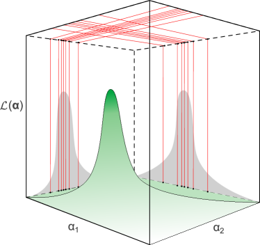
In high-dimensional problems, NS has been criticized for having a sharply decreasing acceptance rate as the likelihood constraint becomes more exclusive Chopin and Robert (2010). Therefore, high-dimensional problems call for an alternative numerical technique. If there is no need to determine the posterior distribution, or if the parameters are so-called “nuisance parameters”, whose value are of no interest, other Monte-Carlo integration methods can be employed. One such method is the vegas algorithm by Lepage Lepage (1978). vegas uses importance sampling: the points are sampled from a proposal distribution which approximates the normalized integrand. The proposal distribution is discretized in the form of an adaptive grid, of which each cell is sampled with an equal probability. This idea is illustrated in Fig. 2. The vegas algorithm is most suitable if the integrand $\mathcal{L}(\bm{\alpha_{M}})$ can be approximated by a separable function.

Figure 2: (color online). The likelihood function $\mathcal{L}(\bm{\alpha})$ (green surface) and the proposal distribution determined by vegas, represented by a grid (red lines) with a number of bins per dimension (here 8).

We have adapted the GNU Scientific Library (GSL) implementation Galassi et al. (2009) of the vegas algorithm to the integrand of the evidence integral, which can assume very small values. This adapted vegas method, which we will refer to as log-vegas, requires a function which returns the natural logarithm of the integrand. The integral is computed while ensuring minimal loss of numerical accuracy that would occur by exponentiation of this function. This measure is indispensable for the integration of small quantities such as a likelihood.

Like any stochastic integration method, the log-vegas algorithm is apt to miss a highly localized maximum. We remedy this by locating the maximum with a genetic algorithm (GA) before performing the integration. We combine a rough search in the full parameter space using a GA and a subsequent fine search in a selected part of the parameter space using the gradient-based methods of minuit, the optimization module of the root library Antcheva et al. (2011). This strategy has been successfully applied to a precise determination of resonance parameters by Ireland et al. Ireland et al. (2004).

The next step is to reduce the integration space to the volume around the peak, with a range of the order of three standard deviations in each dimension. The standard deviation around the maximum can be calculated using the minos routine of minuit Antcheva et al. (2011).

The first question that springs to mind is whether we do not risk underestimating the evidence by limiting the integration domain to the peak volume. We have addressed this concern by applying this method to a toy example, which is detailed in the following Section.

III.5 Toy example

As a proof of principle, we apply the methods outlined in Section III.4 to a tractable and realistic-sized problem. To this end, we use an event described by the function $m_{d}(x)$ which is expressed in terms of a sum of $d$ Legendre polynomials:

$$m_{d}(x) =\sum_{l=0}^{d-1}a_{l}P_{l}(x) x\in[-1,1].$$ (50)

The parameters $a_{l}(l=0,\ldots,d-1)$ are uniformly distributed in in $[-10,10]$ and randomly generated. A mock data set with Gaussian noise is generated from $m_{d}(x)$. The effectiveness of the GA is assessed by testing whether the values $a_{l}$ can be determined from the mock data. In the next step it is investigated whether Bayesian inference can determine which model was used to generate a particular set of mock data. In essence, this amounts to use Bayesian inference to find the dimension $d$ of the model from which the mock data are generated.

We investigate the performance of a GA for models with a complexity ranging from $d=1$ to $d=12$. We consider 4000 data points, a size comparable to that of the world’s $K^{+}\Lambda$ photoproduction data set. For each data set, we attempt to determine the parameters of the underlying model. We scale the population size in the GA linearly with $d$. Due to its random character, convergence times can vary greatly between the different GA runs. To account for this, we have repeated the GA 40 times for each value of $d$, using a different, random set of parameters for each run. We have found that convergence occurs for all trial runs, and that the original parameters are reproduced by the GA with an error per parameter of the order of 0.5%.

Can one determine the model which best describes a given data set from a number of model variants? This key question can be rigorously addressed using Bayesian inference. To illustrate the potential of this method, we generate mock data using the toy model of Eq. (50) at a fixed $d$. In a next step, we try to determine the underlying model (including its dimension $d$) by calculating the Bayesian evidences for different trial models using the log-vegas method. This procedure is tested for data sets generated by models of different complexity: from $d=1$ up to $d=12$.

Figure 3: (color online). The $-\ln{\mathcal{Z}}$ values calculated with the log-vegas algorithm (red squares) and with a combined GA+minuit+log-vegas integration (blue diamonds), for different model dimensions. Each box corresponds with a model with dimension $d$, indicated with the grey band. The mock data set has 100 points.

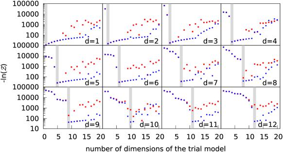
The results of the log-vegas integrations over the entire parameter space are compared to those limited to the peak volume in Fig. 3. We find that the maximum evidence value corresponds to the correct model up to at least $d=12$.

Two striking conclusions can be drawn from Fig. 3. A first observation is that in the low-dimensional problems ($d\lesssim 10$), where the log-vegas result can be considered accurate, the two methods provide a comparable value for the computed integrals. This means that the likelihood in the parameter space outside the peak region is small as compared to the maximum likelihood. Second, the results for high-dimensional models ($d\gtrsim 10$) indicate that the bulk of the evidence is somehow overlooked by the global log-vegas integration. The global integrals for high-dimensional problems can be orders of magnitudes smaller than those that cover only the region around the peak. This indicates that the search space for the log-vegas integration is too large in these high-dimensional problems, and a more dedicated search strategy is required. The results of Fig. 3 indicate that a combined GA+minuit+log-vegas integration strategy is apt to the task of dealing with high-dimensional problems.

IV Background selection in the RPR model

In this section, we apply Bayesian inference to select the optimum model variant for the RPR background amplitude.

IV.1 Parameters of the Reggeized background model

The unknown phases in Eqs. (24) and (25) give rise to several model candidates. The possibility of the $K^{+}$ and $K^{\ast+}$ trajectories having a constant phase is excluded, as this gives rise to a recoil asymmetry $P=0$, which disagrees with the data. In the forthcoming, the remaining three possibilities, namely (rotating $K^{+}$ /rotating $K^{\ast+}$), (rotating $K^{+}$/constant $K^{\ast+}$), and (constant $K^{+}$/rotating $K^{\ast+}$), will be referrred as RR, RC, and CR. Apart from these variants, the background model has three continuous parameters proportional to the product of the strong and electromagnetic couplings,

$$eg_{K^{+}\Lambda p}\qquad, e\,G_{K^{\ast+}}^{v,t}=e\,g_{{K^{\ast+}}\,\Lambda p}^{v,t}\ \kappa_{K^{+}{K^{\ast+}}}\;.$$ (51)

Here, $\kappa_{K^{+}K^{*+}}$ is the transition magnetic moment for $K^{*+}(892)\rightarrow\gamma K^{+}(494)$ decay. Further, the parameters feature the strong coupling constant $g_{K^{+}\Lambda p}$ of the $K^{+}$ trajectory and the tensor and vector couplings $g_{{K^{\ast+}}\,\Lambda p}^{v,t}$ of the $K^{\ast+}$ trajectory.

IV.1.1 Likelihood distribution and data

As discussed in Section III.3, the likelihood distribution of the model parameters with regard to the data is the chi-square distribution of Eq. (47). Recently, the CLAS collaboration published $K^{+}\Lambda$ McCracken et al. (2010) and $K^{+}\Sigma^{0}$ Dey et al. (2010) photoproduction data, featuring high-statistics differential cross-sections and recoil polarizations. The data covers nearly the full angular range and has 1.620 GeV $\lesssim W\lesssim$ 2.840 GeV. The broad energy range makes it a great testing ground for both isobar, Regge and hybrid models such as RPR. Indeed, it includes measurements taken at energies up to $W=2.840$ GeV, which is well above the resonance region.

Sibirtsev et al. Sibirtsev et al. (2007) demonstrated that the $p(\gamma,\pi^{+})n$ and $n(\gamma,\pi^{-})p$ reactions display Regge-like behavior for invariant mass energies as low as 2.6 GeV. Furthermore, Schumacher and Sargsian Schumacher and Sargsian (2011) pointed out that in the small-$|t|$ limit, the differential cross section for $p(\gamma,K^{+})\Lambda$ exhibits Regge-like scaling behavior $\propto s^{-2}$ down to $W\approx 2.3$ GeV. One would therefore expect that a Regge background model optimized to the $W>$ 3 GeV SLAC and DESY data De Cruz et al. (2010), provides a fair description of the $W>$ 2.6 GeV CLAS data. However, this is not the case. Fig. 4 shows the $W>$ 2.6 GeV $K^{+}\Lambda$ photoproduction data, as well as the prediction of the Reggeized background model optimized to the $W>3$ GeV data. Clearly, the Regge model overshoots the CLAS data by at least a factor of 2. There is an obvious discontinuity in the $W$ dependence between the SLAC and CLAS data at $\cos{\theta_{K}^{\ast}}\approx$ 0.865, 0.8, and 0.7.

Figure 4: (color online). The $p(\gamma,K^{+})\Lambda$ differential cross sections as a function of $W$ for various $\cos\theta_{K}^{\ast}$. The dashed lines represent the best model (RR) of Ref. De Cruz et al. (2010) which follows from a Bayesian analysis of the $W>3$ GeV data. The full lines correspond to the best model (RR) from Table 2, optimized against the $2.6$ GeV $<W<3$ GeV CLAS data. The lines and the data are color coded according to $\cos{\theta_{K}^{\ast}}$: from 0.4 (blue) to 1.0 (red). The orange lines correspond to $\cos{\theta_{K}^{\ast}}=0.95$, the other lines have a value that corresponds to the CLAS $\cos{\theta_{K}^{\ast}}$ bins, i. e. 0.865, 0.8, 0.7, 0.6, 0.5 and 0.4. Data are from Refs. McCracken et al. (2010) and Boyarski et al. (1969).

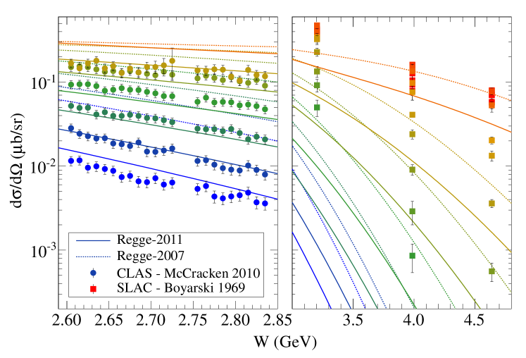
Dey et al. Dey and Meyer (2011) showed that a small set of $p(\gamma,K^{+})\Lambda$ data from CEA Elings et al. (1967) is inconsistent with the CLAS data. They find similar discrepancies between new CLAS data and old high-energy data from SLAC, DESY and CEA for other pseudoscalar meson production reactions. They conclude that there is a persistent normalization issue in the old high-energy differential cross-section data for a number of reactions, including $p(\gamma,K^{+})\Lambda$ and $p(\gamma,K^{+})\Sigma^{0}$. The observations of Fig. 4 add support to these findings.

Because of these observations, we opt to use the data from CLAS, which is consistent with other differential cross-section measurements in the resonance region Bradford et al. (2006); Sumihama et al. (2006), in order to constrain the adjustable parameters in the Reggeized background model. We employ the statistical methods described in Ref. De Cruz et al. (2010), using the 2.6 GeV $<W<$ 3 GeV CLAS data to compute the likelihood function. Below this energy region, resonance contributions become more important Sibirtsev et al. (2007). Because the validity of Regge theory is limited to small $|t|$, we use $\cos{\theta_{K}^{\ast}}>0.35$ data to constrain the background parameters. With these criteria, we retain 132 differential cross sections and 130 recoil polarization $P$. This is over a factor of four more data than for the combined SLAC/DESY data used in the analysis reported in Ref. De Cruz et al. (2010).

IV.1.2 Prior distribution

We opt to use a uniform prior distribution $U$ for the coupling constants of Eq. (51). Under conditions of highly concentrated likelihood, compared to which the prior distribution varies mildly, the likelihood dominates the shape of the posterior distribution Sivia and Skilling (2006). Accordingly, the evidence calculations will not be largely affected by the choice with regard to the shape of the prior distribution. A sensitivity analysis will verify this assumption.

The assumption that SU(3) symmetry is broken at the 20% level yields the following prior ranges for $g_{K^{+}\Lambda p}$  Donoghue and Holstein (1982); Adelseck and Saghai (1990)

$$-4.5\leq \frac{g_{K^{+}\Lambda p}}{\sqrt{4\pi}}\leq-3.0\;.$$ (52)

To our knowledge, for the $K^{\ast+}\Lambda p$ vertex, no reliable theoretical constraints are available Guidal (1997). We choose a uniform distribution between $-$100 and +100 as the initial prior for $\left(G_{K^{\ast+}}^{v},G_{K^{\ast+}}^{t}\right)$. To test the sensitivity of the results to the prior width, the calculations are repeated for a prior width of 2000 and 20000.

IV.1.3 Asymptotic behavior

In the Regge (large $s$ and small $|t|$) limit, one can approximate $s$ by $-u$ for fixed values of $t$. This implies that the energy dependence of the cross section, which follows the power law $s^{\alpha(t)}$ according to Regge theory, can be replaced by $(\frac{s-u}{2})^{\alpha(t)}$ Janssen (2001); Anisovich et al. (2010). In an analysis of $W>3$ GeV data, this difference is not relevant, but at the energies considered here the difference between the two asymptotic behaviors becomes noticeable. Therefore, we have investigated both options using Bayesian inference.

IV.2 Results

IV.2.1 Optimum background model variant

Table 2: Logarithms of the evidence ratios ($\Delta\ln{\mathcal{Z}}\equiv\ln{\left(\mathcal{Z}/\mathcal{Z}_{max}\right)}$) for the six model variants resulting from phase combinations and asymptotic behavior options in the two-trajectory Regge model for $\gamma p\to K^{+}\Lambda$. The prior for the coupling constant $g_{K^{+}\Lambda p}$ is defined by the Eq. (52). The results are listed in order of decreasing probability for the lowest prior width, $\pi=U(-100,100)$ for the $G_{K^{\ast+}}^{t,v}$ couplings.

$K^{+}$ / $K^{*+}$ phase	asymp.	$\pi=U(-100,100)$	$\pi=U(-1000,1000)$	$\pi=U(-10000,10000)$
RR	$s$	0.0	0.0	0.0
RC	$s$	$-32.7$ $\pm$ $1.4$	$-33.5$ $\pm$ $2.7$	$-31$ $\pm$ $13$
RR	$(s-u)/2$	$-359.7$ $\pm$ $1.1$	$-360.8$ $\pm$ $7.2$	$-389$ $\pm$ $57$
RC	$(s-u)/2$	$-432.9$ $\pm$ $1.1$	$-435$ $\pm$ $8.9$	$-472$ $\pm$ $58$
CR	$s$	$-2257.2$ $\pm$ $1.1$	$-2259.3$ $\pm$ $6.4$	$-2282$ $\pm$ $31$
CR	$(s-u)/2$	$-2425.5$ $\pm$ $1.1$	$-2426.3$ $\pm$ $2.6$	$-2440$ $\pm$ $27$

Table 3: Logarithms of the evidence ratios ($\Delta\ln{\mathcal{Z}}\equiv\ln{\left(\mathcal{Z}/\mathcal{Z}_{max}\right)}$) for the six model variants resulting from phase combinations and asymptotic behavior options in the two-trajectory Regge model for $\gamma p\to K^{+}\Lambda$. A deviation of up to 40% from the SU(3) prediction for $g_{K^{+}\Lambda p}$ is allowed. The results are listed in order of decreasing probability for the lowest prior width, $\pi=U(-100,100)$ for the $G_{K^{\ast+}}^{t,v}$ couplings.

$K^{+}$ / $K^{*+}$ phase	asymp.	$\pi=U(-100,100)$	$\pi=U(-1000,1000)$	$\pi=U(-10000,10000)$
RR	$s$	0.0	0.0	0.0
RC	$s$	$-17.8$ $\pm$ $1.1$	$-17.4$ $\pm$ $2.9$	$-15$ $\pm$ $18$
RR	$(s-u)/2$	$-359.7$ $\pm$ $1.0$	$-364.0$ $\pm$ $16.0$	$-387$ $\pm$ $37$
RC	$(s-u)/2$	$-432.7$ $\pm$ $1.2$	$-434.9$ $\pm$ $5.3$	$-474$ $\pm$ $68$
CR	$s$	$-2257.1$ $\pm$ $1.2$	$-2261.5$ $\pm$ $7.7$	$-2272$ $\pm$ $28$
CR	$(s-u)/2$	$-2425.6$ $\pm$ $1.1$	$-2426.3$ $\pm$ $3.0$	$-2426$ $\pm$ $22$

The results of our analysis are listed in Table 2. The data clearly favor a model featuring an $s^{\alpha(t)}$ dependence in the cross section and two rotating trajectories. Indeed, the difference in $\ln{\mathcal{Z}}$ with the second-best variant is $32.7\pm 1.4$, which exceeds the value of 5 required for a decisive statement.

The values of the coupling constants from the best model variant are

$$\frac{g_{K^{+}\Lambda p}}{\sqrt{4\pi}} =-3.6\pm 0.3,$$

$$G_{K^{\ast+}}^{v} =9.0\pm 0.5,$$

$$G_{K^{\ast+}}^{t} =20.9\pm 0.4.$$ (53)

In comparison with the Bayesian analysis of Ref. De Cruz et al. (2010) which was based on the $W>$ 3 GeV data, the tensor coupling $G_{K^{\ast+}}^{t}$ has changed sign, and its magnitude has decreased by about a factor of two. In Ref. De Cruz et al. (2010) which was based on the $W>3$ GeV data, the likelihood hypersurface exhibited a distinct multimodal behavior, with different combinations of the coupling constants’ relative signs giving similar likelihoods. Interestingly, the increased amount of data used here causes the likelihood to be concentrated in only one quadrant of the parameter space in $\left(G_{K^{\ast+}}^{v},G_{K^{\ast+}}^{t}\right)$ and all sign issues for the coupling constants can be resolved.

The expectation value (53) for $g_{K^{+}\Lambda p}$ is close to its SU(3) prediction of Eq. (52). Nevertheless, we have repeated the analyses with a prior for $g_{K^{+}\Lambda p}$ broader than the condition of Eq. (52) in order to to test whether stronger SU(3) flavor symmetry breaking is compatible with the data. The results of this analysis are listed in Table 3. By comparing the results of Tables 2 and 3 one can conclude that the order of the models is unaffected by the operation of broadening the boundaries for the $g_{K^{+}\Lambda p}$ priors. Also the extracted value for $g_{K^{+}\Lambda p}$ is not significantly affected by the broader limits on its prior distribution. Its expectation value becomes $\frac{g_{K^{+}\Lambda p}}{\sqrt{4\pi}}=-3.7\pm 0.3$ which is again compatible with the SU(3) value of $-3.75$.

IV.2.2 High-energy predictions

The high-energy differential cross section as calculated by the best model variant for $p(\gamma,K^{+})\Lambda$ is represented by the full lines in Fig. 4. As expected, the predictions are incompatible with the SLAC data. We attribute this to the normalization discrepancy discussed in Ref. Dey and Meyer (2011) and Section IV.1.1. The polarization observables $\Sigma$ Boyarski et al. (1969); Quinn et al. (1979) and $P$ Vogel et al. (1972) are not sensitive to normalization issues. Predictions for $\Sigma$ at $\omega_{\text{lab}}=16$ GeV are shown in Fig. 5 for $K^{+}\Lambda$. Fig. 5(a) shows the predictions for $P$ at $\omega_{\text{lab}}=5$ GeV. These predictions display an excellent agreement with data. By constraining the Reggeized background at $2.6$ GeV $<W<$ 3 GeV, one can predict $P$ and $\Sigma$ at $W>3$ GeV. This highlights the predictive power of a Regge model at high $W$, and corroborates the assumption that the Reggeized background model can be constrained against $W\gtrsim$ 2.5 GeV observables.

(a)

Figure 5: (color online). Predictions of the best Regge model from Table 2 (full red line) for the $p(\gamma,K^{+})\Lambda$ observables $\Sigma$ and $P$ at $W>3$ GeV, as a function of $-t$. (a) $\Sigma$ at $\omega_{\text{lab}}=16$ GeV. Data are from Ref. Boyarski et al. (1969). (b) $P$ at $\omega_{\text{lab}}=5$ GeV. Data are from Ref. Vogel et al. (1972).

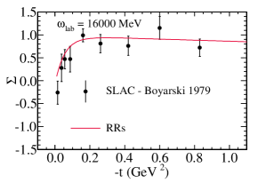
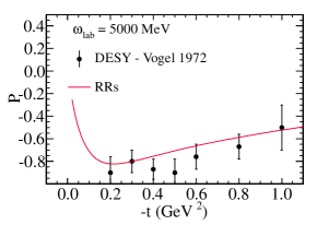
Summarizing the background evaluations, we find that the optimum two-trajectory Regge model for $p(\gamma,K^{+})\Lambda$ features two rotating phases and positive vector and tensor couplings. We also find that an asymptotic $s^{\alpha(t)}$ dependence of the Regge amplitude is preferred over a $\left((s-u)/2\right)^{\alpha(t)}$ one. This model will be referred to as Regge-2011 and determines the prior for the background amplitude of the RPR-2011 model.

V Resonance selection in the RPR model

Given the world’s $p(\gamma,K^{+})\Lambda$ data, this section addresses the following questions: (a) From a proposed set of resonances, what subset features in the most probable model? (b) What is the probability of a proposed resonance $R$? Bayesian inference allows one to answer these questions in a quantitative way.

V.1 Data and resonances

An overview of the available $p(\gamma,K^{+})\Lambda$ data is listed in Table 4. In view of the normalization issue discussed in Section IV, the data from SLAC Boyarski et al. (1969) and DESY Vogel et al. (1972) are not included in the analysis presented below. The total number of data points which we incorporate is 6148, of which 3455 are differential cross sections, 2241 are single and 452 are double polarization results. We stress that after accounting for the error bars all data carry the same weight.

Table 4: Overview of the published experimental data for the reaction $p(\gamma,K^{+})\Lambda$.

Observable	#data	Experiment	Year	Reference
$\frac{d\sigma}{d\Omega}$	56	SLAC	1969	Boyarski Boyarski et al. (1969)
	720	SAPHIR	2004	Glander Glander et al. (2004)
	1377	CLAS	2006	Bradford Bradford et al. (2006)
	12	LEPS	2007	Hicks Hicks et al. (2007)
	2066	CLAS	2010	McCracken McCracken et al. (2010)
$\Sigma$	9	SLAC	1979	Quinn Quinn et al. (1979)
	45	LEPS	2003	Zegers Zegers et al. (2003)
	54	LEPS	2006	Sumihama Sumihama et al. (2006)
	4	LEPS	2007	Hicks Hicks et al. (2007)
	66	GRAAL	2007	Lleres Lleres et al. (2007)
$T$	3	BONN	1978	Althoff Althoff et al. (1978)
	66	GRAAL	2008	Lleres Lleres et al. (2009)
$P$	7	DESY	1972	Vogel Vogel et al. (1972)
	233	CLAS	2004	McNabb McNabb et al. (2004)
	66	GRAAL	2007	Lleres Lleres et al. (2007)
	1707	CLAS	2010	McCracken McCracken et al. (2010)
$C_{x}\;,C_{z}$	320	CLAS	2007	Bradford Bradford et al. (2007)
$O_{x^{\prime}}\;,O_{z^{\prime}}$	132	GRAAL	2008	Lleres Lleres et al. (2009)

We use the differential cross section data measured by the CLAS collaboration Bradford et al. (2006); McCracken et al. (2010) and LEPS Hicks et al. (2007). Due to unresolved discrepancies with other data sets Bydzovsky and Mart (2007), the SAPHIR differential cross-section data Glander et al. (2004) is excluded. This decision is motivated by the fact that the different cross-section measurements by CLAS are internally consistent McCracken et al. (2010) and consistent with the LEPS data Hicks et al. (2007). To date, there is no independent measurement that confirms the SAPHIR data.

The single polarization data consists of two sets of recoil polarization data published by the CLAS collaboration McNabb et al. (2004); McCracken et al. (2010), as well as a set from GRAAL Lleres et al. (2007). The beam asymmetry data used in our analysis includes results from LEPS Zegers et al. (2003); Sumihama et al. (2006); Hicks et al. (2007) and GRAAL Lleres et al. (2007). The included target asymmetries were determined by means of beam-recoil measurements by the GRAAL collaboration Lleres et al. (2009). The included double polarization observables are beam-recoil asymmetries, consisting of $C_{x}$ and $C_{z}$ data by CLAS Bradford et al. (2007) and GRAAL’s measurements of $O_{x^{\prime}}$ and $O_{z^{\prime}}$ Lleres et al. (2009).

The 11 resonances considered in this work and their properties are listed in Table 5. We have “established” as well as “missing” nucleon resonances. As for their quantum numbers, mass, width and transition form factors, we take the values quoted by the PDG. If these are not available, we employ the values determined by analyses based on CQM predictions Mart and Bennhold (1999). This allows us to keep the number of adjustable parameters small.

Table 5: The nucleon resonances evaluated in the analysis given in the notation $L_{2I,2J}(M)$, along with their PDG status, spin ($J$) and parity ($\pi$), Breit-Wigner mass ($M$), width ($\Gamma$), and the uncertainty on the width ($\Delta\Gamma$).

Resonance	PDG status	$J^{\pi}$	$M\text{(MeV)}$	$\Gamma\text{(MeV)}$	$\Delta\Gamma\text{(MeV)}$
$S_{11}(1535)$	${\star}{\star}{\star}{\star}$	$1/2^{-}$	$1535$	$150$	$\pm 25$
$S_{11}(1650)$	${\star}{\star}{\star}{\star}$	$1/2^{-}$	$1650$	$150$	$\pm 20$
$D_{15}(1675)$	${\star}{\star}{\star}{\star}$	$5/2^{-}$	$1675$	$150$	$-20/+15$
$F_{15}(1680)$	${\star}{\star}{\star}{\star}$	$5/2^{+}$	$1685$	$130$	$\pm 10$
$D_{13}(1700)$	${\star}{\star}{\star}$	$3/2^{-}$	$1700$	$100$	$\pm 50$
$P_{11}(1710)$	${\star}{\star}{\star}$	$1/2^{+}$	$1710$	$100$	$-50/+150$
$P_{13}(1720)$	${\star}{\star}{\star}{\star}$	$3/2^{+}$	$1720$	$150$	$-50/+100$
$D_{13}(1900)$	missing	$3/2^{-}$	$1895$	$200$	$-$
$P_{13}(1900)$	${\star}{\star}$	$3/2^{+}$	$1900$	$500$	$-360/+80$
$P_{11}(1900)$	missing	$1/2^{+}$	$1895$	$200$	$-$
$F_{15}(2000)$	${\star}{\star}$	$5/2^{+}$	$2000$	$140$	$-40/+30$

The established four-star resonances listed by the PDG are $S_{11}(1650)$, $D_{15}(1675)$, $F_{15}(1680)$ and $P_{13}(1720)$. The four-star $S_{11}(1535)$ lies below the kaon production threshold, but is included because of its large decay width and its strong predicted coupling to the open strangeness sector An and Saghai (2011). To our knowledge, the contribution of the three-star $D_{13}(1700)$ to $p(\gamma,K^{+})\Lambda$ is confirmed only by the Giessen analysis Shklyar et al. (2005). The $P_{11}(1710)$, which is found in some $K^{+}\Lambda$ analyses, is evaluated as well. The importance of this resonance in the $\pi N$ system was questioned in the most recent SAID analyses Arndt et al. (2006); Workman et al. (2012); Arndt et al. . The $P_{11}(1710)$ has also been identified in the $\pi\pi N$ system Khemchandani et al. (2008).

Furthermore, the two-star resonances $P_{13}(1900)$ and $F_{15}(2000)$ are evaluated. The first of these, $P_{13}(1900)$, was found to couple to $K^{+}\Lambda$ by the Giessen group Shklyar et al. (2007) and by the RPR-2007 model, and accounts for the structure in the energy dependence of the differential cross-section data at $W\approx$ 1900 MeV. Schumacher and Sargsian Schumacher and Sargsian (2011) show that the differential cross section data from CLAS McCracken et al. (2010) supports one or more resonances at $W\approx 2$ GeV. Therefore, the consideration of the $F_{15}(2000)$ seems justified. The missing $D_{13}(1900)$ and $P_{11}(1900)$ resonances earlier introduced in the Ghent isobar model Janssen et al. (2002); Janssen (2001), the RPR-2007 model Corthals et al. (2006); Corthals (2006), and Kaon-Maid Mart and Bennhold (1999) are also evaluated.

A conclusive statement with regard to the $M\approx 1900$ MeV resonances is extremely useful to improve our understanding of the nucleon’s structure. Indeed, quark-diquark models do not predict a resonance at this energy Lichtenberg et al. (1982); Ferretti et al. (2011). By contrast, a number of resonances with a mass of around 1900 MeV is predicted by CQMs Capstick and Roberts (2000); Loring et al. (2001).

V.2 Likelihood function

When calculating the likelihood function against a single data set, one usually does not take systematic errors $\sigma_{\text{sys}}$ into account. However, this course of action is not valid when multiple data sets are combined, as it would result in an underestimate of the likelihood. Assuming that systematic errors are independent and normally distributed, the total errors can be determined by adding the systematic and statistical contributions in quadrature,

$$\sigma_{\text{tot}}^{2}=\sigma_{\text{stat}}^{2}+\sigma_{\text{sys}}^{2}\;.$$ (54)

A more conservative estimate is to add the systematic and statistical errors linearly

$$\sigma_{\text{tot}}^{\prime}=\sigma_{\text{stat}}+\sigma_{\text{sys}}\;.$$ (55)

The numerical calculations for the Bayesian evidences are very demanding and it is prohibitive to run the calculations with various choices for the values of $\sigma_{\text{tot}}$. In what follows, we outline an approximate method which allows one to relate the evidences computed with Eq. (54) to those which use Eq. (55).

Most often, the systematic errors $\sigma_{\text{sys}}$ are computed by taking the squared sum of a number of partial systematic errors $\sigma_{\text{sys}}^{i}$ from different sources. This approach is prone to underestimate the $\sigma_{\text{sys}}$. For a systematic error that is dominated by two errors with a comparable magnitude $\sigma_{\text{sys,1}}\approx\sigma_{\text{sys},2}$, one obtains in the conservative approach

$$\sigma^{\prime}_{\text{sys}}=\sum_{i}\sigma_{\text{sys},i}\approx 2\sigma_{\text{sys},1}\approx\sqrt{2}\sigma_{\text{sys}}.$$ (56)

In a scenario where $\sigma_{\text{stat}}\approx\sigma_{\text{sys}}$, the estimate (54) leads to $\sigma_{\text{tot}}\approx\sqrt{2}\sigma_{\text{stat}}$ and to the following value for a more conservative estimate of $\sigma^{\prime}_{\text{tot}}$

$$\sigma^{\prime}_{\text{tot}}=\sigma_{\text{stat}}+\sigma^{\prime}_{\text{sys}}\approx\sigma_{\text{stat}}+\sqrt{2}\sigma_{\text{sys}}\approx\frac{1+\sqrt{2}}{\sqrt{2}}\sigma_{\text{tot}}.$$ (57)

One can convert the $\mathcal{Z}$ values computed with the errors of Eq. (54) into a $\mathcal{Z}^{\prime}$ which use $\sigma^{\prime}_{\text{tot}}$. If the errors are multiplied by $c$, the log-chi-square distribution $\ln\mathcal{L}(\bm{\alpha}_{M})$ of Eq. (49) scales as

$$S(k,\chi_{R}^{2}(\bm{\alpha}_{M}),c) \equiv\ln\left(\dfrac{\mathcal{L}(\bm{\alpha}_{M})}{\mathcal{L}^{\prime}_{c}(\bm{\alpha}_{M})}\right)$$

$$=(k-2)\ln{c}-\chi^{2}_{R}\frac{k}{2}\;\frac{c^{2}-1}{c^{2}}.$$ (58)

Here, $k$ denotes the number of degrees of freedom, $\chi_{R}^{2}\equiv\chi^{2}/k$ is the reduced chi-squared as computed with the values $\sigma_{\text{tot}}$. One can estimate the evidence resulting from the scaled likelihood function $\mathcal{L}^{\prime}_{c}(\bm{\alpha}_{M})$ as follows. Inserting a uniform prior into the Eq. (40) yields the following expression for $\mathcal{Z}$

$$\mathcal{Z}=\dfrac{1}{\Delta}\int_{\bm{\alpha}_{\text{0}}}^{\bm{\alpha}_{\text{1}}}\mathcal{L}(\bm{\alpha})d\bm{\alpha}\approx\dfrac{1}{\Delta}\int_{D}\mathcal{L}(\bm{\alpha}_{\text{max}})d\bm{\alpha},$$ (59)

where $\Delta\equiv\prod_{i}\left(\Delta{\alpha}_{i}\right)$ is the volume of the prior hypercube. Indeed, if $\mathcal{L}(\bm{\alpha})$ is the chi-square distribution with $\chi_{R}^{2}(\bm{\alpha})$ far from its optimal value of 1 (e.g. $\chi_{R}^{2}=4$), it falls rapidly with increasing $\chi^{2}(\bm{\alpha})$, and the bulk of the likelihood originates from a volume $D$ where $\mathcal{L}(\bm{\alpha})\approx\mathcal{L}_{\text{max}}$, or $\chi_{R}^{2}(\bm{\alpha})\approx\chi^{2}_{R,\text{min}}$, as illustrated in Fig. 6.

Figure 6: The integral over the likelihood function (black curve) can be approximated by the contribution for which $\mathcal{L}(\alpha)\approx\mathcal{L}_{\text{max}}$, or conversely, for which $\chi^{2}(\alpha)=\chi^{2}_{\text{min}}$ (grey box).

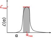
By expressing the corrected likelihood $\mathcal{L}^{\prime}_{c}(\bm{\alpha})$ in terms of the likelihood $\mathcal{L}(\bm{\alpha})$ and the scaling factor of Eq. (58), the expression for $\mathcal{Z}^{\prime}$ becomes

$$\mathcal{Z^{\prime}} \approx\dfrac{1}{\Delta}\int_{D}\mathcal{L}^{\prime}_{c}(\bm{\alpha_{\text{max}}})d\bm{\alpha}$$

$$\approx\dfrac{1}{\Delta}\int_{D}\mathcal{L}(\bm{\alpha}_{\text{max}})e^{-S\left(k,\chi_{R}^{2}({\bm{\alpha}_{\text{max}})},c\right)}\;d\bm{\alpha}$$ (60)

$$\approx\mathcal{Z}\;e^{-S\left(k,\chi^{2}_{R,\text{min}},c\right)},$$ (61)

which yields our final result

$$\ln\mathcal{Z}^{\prime} \approx\ln\mathcal{Z}-S\left(k,\chi^{2}_{R,\text{min}},c\right).$$ (62)

The expression (54) for $\sigma_{\text{tot}}$ presupposes stringent independences between the various contributions. The $\sigma_{\text{tot}}^{\prime}$ of Eq. (55) provides a more conservative estimate of the evidence. In order to avoid overestimating the amount of information that is provided by the data, we will use $\sigma_{\text{tot}}^{\prime}$ in the forthcoming analyses.

V.3 Identifying the resonance content of $p(\gamma,K^{+})\Lambda$

The 11 proposed resonances of Table 5 give rise to $2^{11}=2048$ model variants. The Bayesian evidence $\mathcal{Z}^{\prime}$ of Eq. (62) is computed for each model, resulting in a map of the RPR model space, shown in Fig. 7.

Figure 7: (color online). The evidences $(-\ln{\mathcal{Z}^{\prime}})$ of the 2048 model variants in the RPR model space (blue circles), as a function of the number of free $N^{\ast}$ parameters. The latter value equals the number of $N^{\ast}$ couplings plus one for the $\Lambda_{R}$. The smaller the value of $-\ln\mathcal{Z}^{\prime}$ the higher the evidence. The best model for a fixed number of parameters is indicated with a red square. The model with the highest evidence, RPR-2011, is denoted with a black diamond.

Figure 8: (color online). The evidences $(-\ln{\mathcal{Z}^{\prime}})$ of the 2048 model variants in the RPR model space (blue circles). The purple diamonds correspond with the subset of models which contain the resonance indicated in the top right corner of each panel.

Figure 9: (color online). The evidences $(-\ln{\mathcal{Z}^{\prime}})$ of the 2048 model variants in the RPR model space (blue circles). The orange diamonds correspond with the subset of models which do not contain the resonance indicated in the top right corner of each panel.

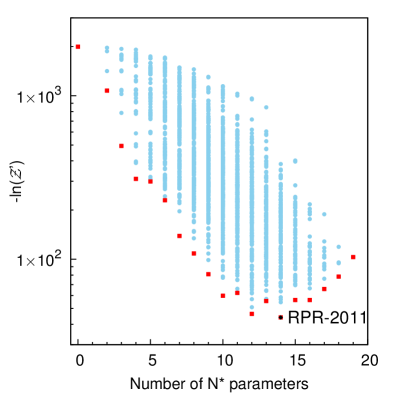
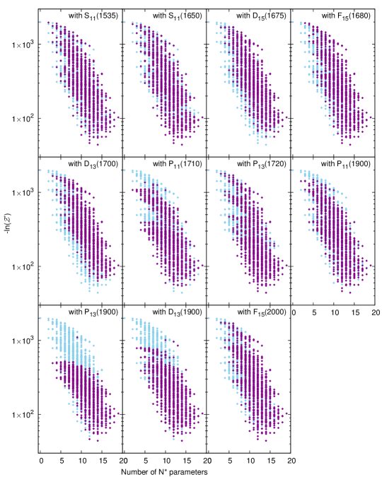
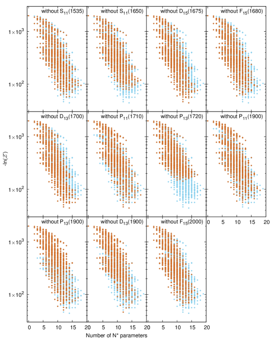
The parameters of the Reggeized background are assigned localized priors of 20% around the values determined in Section IV. Therefore, the total number of adjustable parameters is the sum of the number of $N^{\ast}$ couplings, of the three background parameters, and of the cut-off value $\Lambda_{R}$ of Eq. (37). The number of fitted $N^{\ast}$ couplings extends from 1 (one spin-1/2 coupling) to 18 ($4\times 1$ spin-1/2, $4\times 2$ spin-3/2, $3\times 2$ spin-5/2 couplings). We adopt one common value for $\Lambda_{R}$ for all resonances with a uniform prior between 1.0 and 3.5 GeV. When selecting a prior distribution, it is good practice to ignore the data. Often an overestimation of the evidence results from determining the likelihood and the prior with a particular data set. In this work, the ranges of the prior distributions of the resonance couplings are selected on the basis of naturalness arguments. Indeed, the contribution of a single resonance is unlikely to exceed the total $p(\gamma,K^{+})\Lambda$ cross section ($\sigma\approx 5\mu b$) by a large factor. We performed calculations of the total cross sections ($\sigma_{R}$) in a model which includes a single resonance $R$ and the Reggeized background. It is observed that the criterion $\sigma_{R}<25\mu b$ leads to absolute values of the coupling constants smaller than 100 in the adopted units convention. Therefore, we adopt a uniform distribution for the priors of the resonance coupling constants in the range $[-100,100]$.

Jeffreys’ scale allows us to determine the “best” model from the 2048 variants. The model with the highest evidence has $14$ $N^{\ast}$ parameters (13 couplings and $\Lambda_{R}$) and features the $S_{11}(1535)$, $S_{11}(1650)$, $F_{15}(1680)$, $P_{13}(1720)$, $P_{11}(1900)$, $F_{15}(2000)$, and the missing $D_{13}(1900)$ and $P_{13}(1900)$. This model variant will be referred to as RPR-2011 De Cruz et al. (2012). The “second-best” model has two parameters less due to the absence of the $D_{13}(1900)$. The difference in $-\ln\mathcal{Z}$ between the “best” and “second-best” models is 2.3. This corresponds to significant to strong evidence in favor of RPR-2011. The difference with the other models is at least 6.8, which is consistent with decisive evidence for RPR-2011.

Figure 10: The relative resonance probabilities of Eq. 63 for each resonance listed in Table 5.

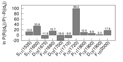
In a next step, one can quantify the probability of each resonance separately by evaluating $P\left(R\;|\left\{d_{k}\right\}\right)$ of Eq. (46). Fig. 8 visualizes which models are included in the sum. It is also instructive to calculate $P\left(\sim R\;|\left\{d_{k}\right\}\right)$, the probability that a resonance is not required to describe the reaction. The calculation of this quantity is completely analogous to Eq. (46). In Fig. 9, the models which do not include a resonance $R$ are visualized for each proposed resonance.

The probability ratios

$$\ln\left(P\left(R\;|\left\{d_{k}\right\}\right)/P\left(\sim R\;|\left\{d_{k}\right\}\right)\right),$$ (63)

are plotted in Fig. 10. A positive ratio indicates that the probability that the resonance $R$ contributes to the reaction $p(\gamma,K^{+})\Lambda$ is greater than the probability that it does not. Conversely, a negative ratio means that the data does not support the possibility that $R$ contributes to the reaction.

The results indicate that the resonances in RPR-2011 are those that have a positive probability ratio. Moreover, the two resonances with the highest probabilities are $P_{13}(1720)$ and $S_{11}(1650)$. These are the two resonances that are also deemed important for the description of $p(\gamma,K^{+})\Lambda$ by most other models. There is decisive evidence that the $D_{15}(1675)$, $D_{13}(1700)$, and $P_{11}(1710)$ are not required to describe the $p(\gamma,K^{+})\Lambda$ data. With regard to the resonance content in the 1800-2000 MeV mass range several suggestions have been in the literature, but no consensus has been reached. We have evaluated four states in that mass region (Table 5): two have a two-star status and two are labeled as “missing”. Our analysis provides decisive evidence for three of these states: $P_{13}(1900)$, $P_{11}(1900)$, and $F_{15}(2000)$. Note that the evidence for the “missing” $D_{13}(1900)$ is significant to strong, but not decisive.

Figure 11: (color online). Angular dependence of the differential cross section at various incident photon energies $\omega_{\text{lab}}$. The full red line represents the RPR-2011 model, the blue dashed line corresponds with Regge-2011. Data are from Refs. Glander et al. (2004); Hicks et al. (2007); Bradford et al. (2006); McCracken et al. (2010).

Figure 12: (color online). Angular dependence of the single polarization observables: beam asymmetry $\Sigma$ (top row), recoil polarization $P$ (middle row), and target asymmetry $T$ (bottom row), at various incident photon energies $\omega_{\text{lab}}$. Line conventions as in Fig. 11. Data are from Refs. Zegers et al. (2003); McCracken et al. (2010); McNabb et al. (2004); Lleres et al. (2009, 2007).

V.4 Photoproduction with RPR-2011

The $p(\gamma,K^{+})\Lambda$ observables presented in this subsection are calculated with the RPR-2011 model parameters fixed at their maximum likelihood values. The RPR-2011 results are compared to the Reggeized background model Regge-2011 that was determined in Section IV. From the difference between the Regge-2011 and the RPR-2011 results one can infer conclusions about the role of the resonances for the various observables.

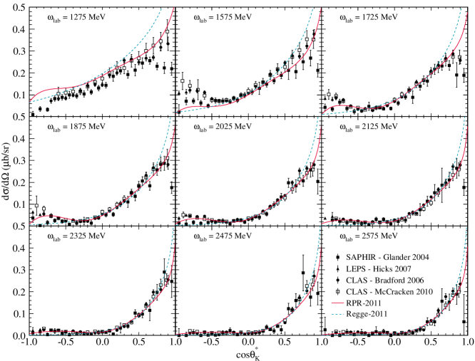
The $p(\gamma,K^{+})\Lambda$ differential cross section is displayed as a function of $\cos\theta_{K}^{\ast}$ in Fig. 11. RPR-2011 provides a good description over a wide range of kinematics. For the lowest energies and backward angles there are deviations between the model and the data, hinting at possible missing dynamics such as $u$-channel contributions. It is striking that the $t$-channel background of the Regge-2011 model already provides a reasonable description of the gross features of both the $\omega_{lab}$ and $\cos\theta_{K}^{\ast}$ dependence of the differential cross sections. The biggest effect from the resonance contributions is observed at the forward and backward kaon angles.

Both RPR-2011 and Regge-2011 models exhibit a steep rise at extremely forward angles. At the three lowest $\omega_{lab}$ energies considered in Fig. 11 the inclusion of the resonances softens this rise and improve the goodness of the fit to the data. Note that the SAPHIR data (Fig. 1) suggest a plateau at forward kaon angles and that this feature is absent in the CLAS data.

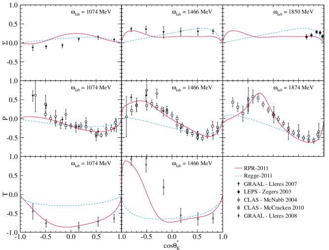
The angular dependence of the single-polarization observables $\Sigma,P,T$ is shown for three representative energies in Fig. 12. The $\Sigma,P,T$ receive stronger contributions from the $N^{\ast}$’s than the differential cross sections. In contrast to the high-energy situation considered in Fig. 5, the photon asymmetries in the resonance region are relatively small. The Regge-2011 reproduces the trend of increasing $\Sigma$ with growing $\omega_{lab}$. The inclusion of the $N^{\ast}$’s does not lead to a considerably improved quality of the fit. The recoil polarization $P$ and target polarization $T$ are highly sensitive to the resonance contributions.

Figure 13: (color online). Angular dependence of the beam-recoil double polarization observables with circular beam polarization, $C_{x}$ and $C_{z}$ (top rows), and with oblique beam polarization, $O_{x^{\prime}}$ and $O_{x^{\prime}}$ (bottom rows), at various incident photon energies $\omega_{\text{lab}}$. Line conventions as in Fig. 11. Data are from Refs. Lleres et al. (2009); Bradford et al. (2007).

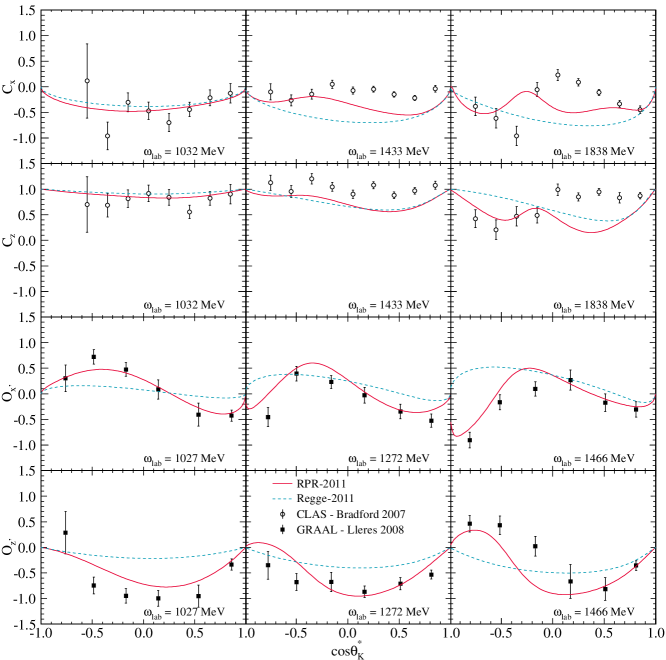
We now turn our attention to the double polarization observables. We stress that they represent but 7% of the total amount of data and that we give each data point an equal weight. As the bulk of the data is in the differential cross sections and to a lesser extent in the single polarization observables, the double polarization observables represent stringent tests of the RPR-2011 model. Perhaps somewhat surprisingly, Regge-2011 provides a good approximation to the double-polarization observables $C_{x}$ and $C_{z}$. The observed trends $C_{z}\approx 1$ and $C_{x}\approx C_{z}-1$ Schumacher (2008) are well reproduced by both the Reggeized background (Regge-2011) and RPR-2011. This observation hints at the fact that the $C_{x},C_{z}$ are very background dominated. A large sensitivity to resonance contributions is observed for $O_{x^{\prime}}$ and $O_{x^{\prime}}$, which are considerably better described by RPR-2011 than by Regge-2011.

Figure 14: The unseparated structure functions $\sigma_{T}+\varepsilon\,\sigma_{L}$ for $p(e,e^{\prime}K^{+})\Lambda$ at $\cos\theta_{K}^{\ast}\approx 1$ as a function of $W$, at $Q^{2}=2.9$ GeV² (left panel) and as a function of $Q^{2}$, at $W=2160$ MeV (right panel). Line conventions as in Fig. 11. Data are from Refs. Brown et al. (1972); Bebek et al. (1974, 1977).

Figure 15: The separated structure functions $\sigma_{T}$ (top panels) and $\sigma_{L}$ (bottom panels) for $p(e,e^{\prime}K^{+})\Lambda$ at $\cos\theta_{K}^{\ast}\approx 1$ as a function of $W$, at $Q^{2}=1.90$ GeV² (left panels) and at $Q^{2}=2.35$ GeV² (right panels). Line conventions as in Fig. 11. Data are from Ref. Coman et al. (2010).

V.5 Electroproduction predictions with RPR-2011

Electroproduction reactions have the potential to probe the hadron’s electromagnetic substructure. The existence of this substructure can be parametrized by introducing a $Q^{2}$ dependence in the electromagnetic coupling constants. In addition, the $p(e,e^{\prime}K^{+})\Lambda$ reaction dynamics becomes sensitive to longitudinal couplings. In part, these couplings arise naturally from the photoproduction amplitudes when gauge invariance is imposed. A peculiar class of longitudinal couplings vanishes for photoproduction reactions and cannot be constrained against real-photon data. The latter class of longitudinal couplings are neglected in the RPR model. In brief, we fix the basic reaction mechanism to the $p(\gamma,K^{+})\Lambda$ data and treat the electroproduction data as a test of the model. Thereby, we make some reasonable assumptions with regard to the electromagnetic form factors of the $t$-channel kaons and $s$-channel $N^{\ast}$’s. Such an extrapolation of the $p(\gamma,K^{+})\Lambda$ amplitude to $p(e,e^{\prime}K^{+})\Lambda$ has been shown as reasonably successful for the RPR-2007 model Corthals et al. (2007a). We use the same $N^{\ast}$ helicity amplitudes (HA) as in Ref. Corthals et al. (2007a). Also the transition form factors for the spin-$1/2$ particles are those from Ref. Corthals et al. (2007a). The transition form factors for the spin-$3/2$ particles are derived from the consistent Lagrangians of Eqs. (32)–(33). For the spin $3/2$ and $5/2$ particles, the HA are calculated in the Bonn constituent quark model Loring et al. (2001), and the transition form factors are derived using Eqs. (34)–(35).

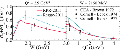
A comparison between recent low $Q^{2}=0.030-0.055$ GeV² measurements and RPR-2011 predictions are contained in Ref. Achenbach et al. (2012). It was observed that RPR-2011 provides a fair description of those data. Unseparated structure functions $\sigma_{T}+\varepsilon\,\sigma_{L}$ at very forward kaon angles obtained in the 1970s are shown as a function of $W$ and $Q^{2}$ in Fig. 14 together with Regge-2011 and RPR-2011 predictions. Obviously, at $\cos\theta_{K}^{\ast}\approx 1$ the major impact of the intermediate resonances is to reduce the cross section by some modest factor. This is in line with the observations made for the real-photon differential cross sections of Fig. 11. The electromagnetic form factors of the intermediate resonances reduce the effect of the $N^{\ast}$’s with growing photon virtuality $Q^{2}$. The RPR-2011 model provides a fair prediction for both the $Q^{2}$ and $W$ dependence of the data.

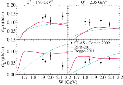
Fig. 15 shows the energy dependence of the separated structure functions $\sigma_{L}$ and $\sigma_{T}$. In line with the data, RPR-2011 predicts a $\sigma_{L}$ and $\sigma_{T}$ of almost equal magnitude. The $\sigma_{T}$ appears to be systematically underpredicted while $\sigma_{L}$ is somewhat overpredicted. The fair reproduction of both the magnitude and the $W$ dependence of $\sigma_{L}$ provides support for our assumptions with regard to the longitudinal couplings.

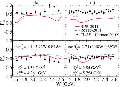
Predictions for the transferred polarisation are presented in Fig. 16. The Reggeized background model Regge-2011 as it was determined in Sect. IV.2.1 predicts the flat $W$ dependence and the magnitude of $P^{\prime}_{z}\approx 0.0$ and $P^{\prime}_{x}\approx 0.5$. For $P^{\prime}_{z}$, the introduction of resonances worsens the quality of the agreement with the data obtained in Regge-2011. For $P^{\prime}_{x}$ the effect of the $N^{\ast}$ is smaller and the quality of the agreement is better than for $P^{\prime}_{z}$.

Figure 16: Transferred polarisation $P^{\prime}_{z}$ (top panels) and $P^{\prime}_{x}$ (bottom panels) as defined in Table III of Ref. Carman et al. (2009) for $p(\vec{e},e^{\prime}K^{+})\vec{\Lambda}$ at (a) $Q^{2}=1.56$ GeV² and $\epsilon_{1}^{lab}$=4.261 GeV (a), and (b) $Q^{2}=2.54$ GeV² and $\epsilon_{1}^{lab}$=5.754 GeV. The $W$ dependence of $\cos\theta_{K}^{\ast}$ can be captured by the following functions: (a) $\cos\theta_{K}^{\ast}=-4.1+3.92W-0.84W^{2}$, and (b) $\cos\theta_{K}^{\ast}=-3.74+3.48W-0.69W^{2}$. Line conventions as in Fig. 11. Data are from Ref. Carman et al. (2009).

VI Conclusion

The RPR framework conjoins a Reggeized $t$-channel background with tree-level $s$-channel nucleon resonances from an isobar approach into an economical model for kaon photoproduction in and above the resonance region. The RPR model clearly separates nonresonant from resonant amplitudes which is an asset when searching for the properties of those (missing) resonances which contribute to $p(\gamma,K^{+})\Lambda$.

We have used Bayesian inference to perform model selection both with regard to the resonant and nonresonant content of the RPR framework. It was shown that the Bayesian evidence $\mathcal{Z}$ is a quantitative measure for a model’s fitness given data. The computation of $\mathcal{Z}$ requires involving multidimensional integrals which demand dedicated numerical methods. To that purpose we have proposed the “GA+minuit+log-vegas” integration strategy. With this method one can reliably compute $\mathcal{Z}$ for models with a moderate number of adjustable parameters such as the RPR framework.

First, the most probable model variant for the Reggeized background was determined against the 2.6 GeV$<W<$3.0 GeV data. This involves the determination of three continuous and two discrete adjustable parameters. The extracted value for $g_{K^{+}\Lambda p}$ is compatible with the one predicted by SU(3) symmetry. Next, we have considered a set of 11 nucleon resonances to determine the optimum resonant contribution in the RPR $p(\gamma,K^{+})\Lambda$ framework. To this end, the Bayesian evidence was calculated for all 2048 model variants resulting from the various resonance combinations. The model with the highest evidence, dubbed RPR-2011, includes the resonances $S_{11}(1535)$, $S_{11}(1650)$, $F_{15}(1680)$, $P_{13}(1720)$, $P_{11}(1900)$, $F_{15}(2000)$, $D_{13}(1900)$, and $P_{13}(1900)$. An evaluation of the individual resonances’ probabilities reveals that the two resonances with the highest evidence of contributing to $p(\gamma,K^{+})\Lambda$ are the $S_{11}(1650)$ and $P_{13}(1720)$. There is decisive evidence that the $D_{15}(1675)$, $D_{13}(1700)$, and $P_{11}(1710)$ are not required to describe the current $p(\gamma,K^{+})\Lambda$ world’s data. The computed evidence for the two-star $P_{13}(1900)$, the two-star $F_{15}(2000)$, and the “missing” $P_{11}(1900)$ is decisive, whereas for the “missing” $D_{13}(1900)$ it is significant, but not decisive.

After fixing the basic reaction reaction mechanism to the $p(\gamma,K^{+})\Lambda$ data, the electroproduction data serve as a test of the model. In general our predictions for the electroproduction data are reasonably good which proves that the RPR-2011 model possesses predictive power and goes beyond a mere analysis framework. Therefore, we consider RPR-2011 as an efficient and robust model which can, for example, be used as an elementary production operator in strangeness production reactions involving the deuteron and finite nuclei.