Second- and First-Order Phase Transitions in CDT
J. Ambjørn, S. Jordan, J. Jurkiewicz and R. Loll
a The Niels Bohr Institute, Copenhagen University
Blegdamsvej 17, DK-2100 Copenhagen Ø, Denmark.
email: ambjorn@nbi.dk
b Institute for Theoretical Physics, Utrecht University,
Leuvenlaan 4, NL-3584 CE Utrecht, The Netherlands.
email: s.jordan@uu.nl, r.loll@uu.nl
c Institute of Physics, Jagellonian University,
Reymonta 4, PL 30-059 Krakow, Poland.
email: jurkiewicz@th.if.uj.edu.pl
d Perimeter Institute for Theoretical Physics,
31 Caroline St. N., Waterloo, Ontario, Canada N2L 2Y5.
email: rloll@perimeterinstitute.ca
Abstract
Causal Dynamical Triangulations (CDT) is a proposal for a theory of quantum gravity, which implements a path-integral quantization of gravity as the continuum limit of a sum over piecewise flat spacetime geometries. We use Monte Carlo simulations to analyse the phase transition lines bordering the physically interesting de Sitter phase of the four-dimensional CDT model. Using a range of numerical criteria, we present strong evidence that the so-called A-C transition is first order, while the B-C transition is second order. The presence of a second-order transition may be related to an ultraviolet fixed point of quantum gravity and thus provide the key to probing physics at and possibly beyond the Planck scale.
1 Introduction
The relation between general relativity and quantum physics is still far from being understood, despite decades of research. Expanding the gravitational field around a fixed background geometry results in a perturbatively nonrenormalizable theory. The best one can do within this conventional setting is to view the quantum field theory as an effective field theory up to a certain energy scale [1, 2]. However, because of their extreme smallness, it remains unclear whether any quantum corrections one can compute in the range where this effective framework is reliable can be related to observable quantities, even in principle [3].
In order to define a theory which is UV-complete one has to go beyond ordinary perturbative quantum field theory, either by modifying or extending the notion of “quantum fields” (as happens in supergravity, string theory or noncommutative field theory, say), or by trying to define a quantum field theory of gravity nonperturbatively (as, for example, in lattice or loop quantum gravity). In this article we will be following a nonperturbative route to quantization via the method of Causal Dynamical Triangulations (CDT), which falls into the latter category.
One explanation for why quantum gravity could be well-defined nonperturbatively, despite its lack of perturbative renormalizability, is given by the so-called asymptotic safety scenario. Its general framework was originally formulated by Weinberg [4], and is based on the hypothesis that the quantum field theory of four-dimensional gravity possesses a non-Gaussian ultraviolet fixed point under the flow of the renormalization group. The existence of such a UV fixed point is suggested by a -expansion in the dimensionality of spacetime, starting from the observation that two-dimensional “gravity” is formally a renormalizable theory [5], an observation later corroborated in [6] (for a summary of these results, see [7]). Further support, which does not rely on perturbing around , comes from using functional renormalization group methods, first applied in the context of gravity in a seminal paper by Reuter [8]. Explicit numerical computations of the renormalization group trajectories require a truncation of the infinite tower of higher-order curvature terms in the gravitational Lagrangian. By now, numerous truncations have been studied, which all point to the existence of a fixed point [9] (see [10] for a recent review).
Independent evidence for the asymptotic safety of gravity – if it is realized – could come from a nonperturbative path integral quantization of gravity. In order to make the path integral well defined one usually discretizes the space of field configurations, which for pure gravity is the space of all spacetime geometries. This can be conveniently achieved by representing spacetime geometries in terms of piecewise flat, triangulated manifolds with distributional curvature assignments, leading to the simplicial approaches to quantum gravity, such as quantum Regge calculus and dynamical triangulations (DT) (see [11] for a review). In what follows we will study an improved, Lorentzian version of the latter, known as Causal Dynamical Triangulations (CDT) (see [12] for reviews).
A crucial and nontrivial requirement for all nonperturbative approaches to quantum gravity is that they must reproduce well-established classical behaviour of gravitational physics in the low-energy limit. In this respect CDT has had some remarkable successes. Numerical simulations of the model have demonstrated the dynamical emergence of a four-dimensional classical universe as the ground state of the system, even though no background was ever put in by hand [14]. In addition, a more detailed analysis revealed that the effective action for the scale factor of the universe can be matched to a minisuperspace action describing a quantum de Sitter spacetime, including linearized quantum fluctuations [15]. By contrast, the present piece of work will focus on the short-distance behaviour of quantum gravity, defined through CDT.
In the following section we will recap some essential ingredients of the CDT approach, to set the stage for the subsequent discussion of its phase structure. In Sec. 3 we recall some properties of the phase diagram and describe our method of locating the phase transitions quantitatively. In Sec. 4 we turn to the determination of the order of two of the phase transitions, the transition line between phases A and C, and between phases B and C. The fact that the B-C transition appears to be of second order has been announced recently in [16]. Finally, our conclusions are presented in Sec. 5.
2 Causal Dynamical Triangulations
We begin by summarizing some important aspects of CDT, which are relevant for our subsequent discussion of its phase structure, and recommend consulting [17, 18, 19] for more detailed information. The primary idea behind CDT is to quantize gravity in the path-integral formalism, and is best illustrated in terms of the analogous quantization of the nonrelativistic particle. In order to properly define the path integral for the latter one can discretize time by introducing a unit time interval of length , and consider only paths which consist of a contiguous sequence of linear segments, one for each time interval. Continuum quantum physics is then recovered by taking the limit as of the regularized path integral over the ensemble of piecewise linear paths.
When generalizing from nonrelativistic particle physics to quantum gravity, the sum over piecewise linear (read: piecewise straight) particle paths becomes a sum over piecewise linear (read: piecewise flat) spacetime geometries. At this point one needs a concise definition of the (regularized) space of geometries to be summed over. The distinguishing feature of CDT, compared to other, similar approaches, is that all geometries in its configuration space are equipped with a discrete foliation. Each leaf – labeled by a discrete lattice time – is a piecewise linear spatial hypersurface of a given, fixed topology . More precisely, each spatial hypersurface is a simplicial manifold built out of equilateral flat tetrahedra with link length , together forming a three-dimensional triangulation. Adjacent spatial hypersurfaces are then connected with the help of four-simplices, in such a way that the whole spacetime becomes a four-dimensional simplicial manifold of topology . In practice we use and furthermore impose periodic boundary conditions in the time direction, such that the spacetime topology becomes , but this should be regarded merely as a choice of convenience.
The resulting four-dimensional triangulation forms a simplicial complex, consisting of vertices, links, triangles, tetrahedra and four-simplices. The Lorentzian nature of the metric properties of the triangulations implies a more refined categorization of their elementary building blocks. There are two different types of links, depending on whether their endpoints lie on the same hypersurface (leading to spatial links) or on two neighbouring hypersurfaces (resulting in timelike links). In CDT quantum gravity we allow these two types to have different absolute length and define the (squared) length of the timelike links to be , with a relative scaling parameter . Consequently, higher-dimensional (sub-) simplices of a CDT geometry also come in different varieties, depending on the space- or timelike character of their one-dimensional subsimplices.
The path integral now becomes a sum over all geometrically inequivalent triangulations of this type with a fixed number of time steps. As an action we use the Einstein-Hilbert action, which has a natural realization on piecewise linear geometries, the so-called Regge action [20]. The corresponding model in two dimensions can be solved analytically [21], but already the three-dimensional model has only been solved partially and for restricted classes of triangulations [22, 23]. In four dimensions analytical methods are mostly unavailable and one must resort to Monte Carlo simulations to extract physical results. To do so one needs to convert the path integral into a statistical partition function by applying a Wick rotation.
Because of the presence of a foliation and an associated global notion of time one can perform a Wick rotation at the level of the geometries by simply rotating in the lower-half complex plane. The Regge action changes accordingly and becomes the Euclidean Regge action
| (1) | |||||
where , and denote the numbers of vertices, four-simplices and four-simplices of type (4,1) (with four vertices on one hypersurface and the fifth on a neighbouring hypersurface). The three couplings , and can be expressed as functions of the bare gravitational coupling, the bare cosmological coupling and the asymmetry parameter introduced above. By defining one obtains the version of the Euclidean Regge action which is ultimately implemented in the computer simulations, namely,
| (2) |
where we have grouped together the terms proportional to . For later convenience we introduce the notation for the quantity conjugate to in the action.
In this way the path integral of quantum gravity is turned into a statistical partition function. We will use the freedom to switch to a different ensemble, obtained by holding fixed – measuring the size (the total discrete spacetime volume) of the system – instead of its conjugate . We therefore treat as a finite-size scaling parameter which does not appear in the phase diagram of the putative continuum theory. The remaining two couplings and span the phase diagram of the system, which we will explore in the next section.
3 The phase diagram of CDT
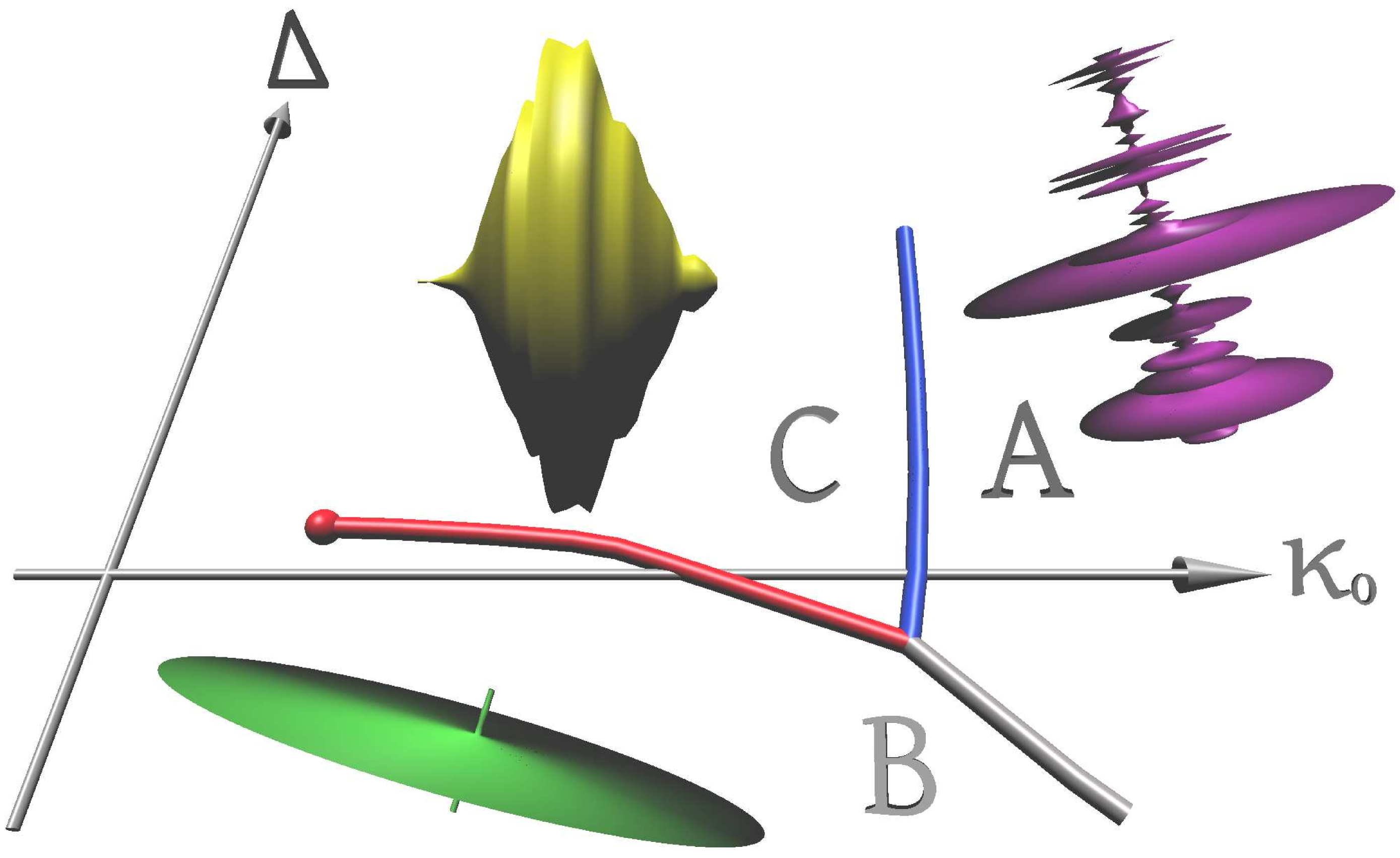
The first, qualitative description of the CDT phase diagram appeared in [17], followed more recently by a quantitative and more detailed analysis in [24]. The new visualization of the phase diagram shown in Fig. 1 is based on phase transition data from the latter. The phase diagram contains three phases, labelled A, B and C [17]. They can be distinguished by looking at a particular feature of the large-scale geometry of their ground state, the spatial volume profile , which measures the three-volume in lattice units as a function of proper time .
Representative profiles have been visualized in Fig. 1 by rotating the function around the -axis, thereby creating a body of revolution. The average geometry (“average” in the sense of expectation values) found in phase C exhibits the scaling behaviour of a genuinely four-dimensional universe, whose average volume profile is consistent with a Euclidean de Sitter spacetime [15, 19]. The situation in the other phases is very different. The typical volume profile of a configuration in phase A consists of an essentially uncorrelated sequence of spatial slices, while the configurations in phase B are characterized by an almost vanishing time extension, in the sense that almost the entire volume of the system is concentrated around a single spatial slice.
We should mention at this stage that several qualitative features of the CDT phase diagram bear a striking resemblance to those of a similar diagram in so-called Hořava-Lifshitz gravity [25], as has been pointed out elsewhere [26, 24]. Trying to understand whether this indicates a deeper relation between the two quantum-gravitational frameworks provides an additional incentive for performing a more detailed quantitative analysis of the phase diagram, as we are doing here.

Fig. 2 shows the quantitative phase diagram, measured at system size . The location of the phase transitions depends on the system size: when is increased, the A-C transition moves towards larger values of , while the B-C transition moves towards larger values of . Using finite-size scaling techniques it is possible to determine the location of transition points for infinite four-volume.
Before embarking on a detailed analysis of the CDT phase transitions, let us comment on some technical issues with regard to measuring the location of a phase transition. The very notion of a phase transition point is of course ambiguous for finite systems, because strictly speaking phase transitions can only occur in the limit of infinite size. For example, consider the susceptibility associated with some observable . Plotting the function near the B-C transition, one will find that it has a maximum at some value . The location of this maximum can be used as a definition of the transition point, but one must keep in mind that its precise value will in general depend weakly on .
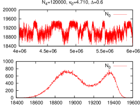
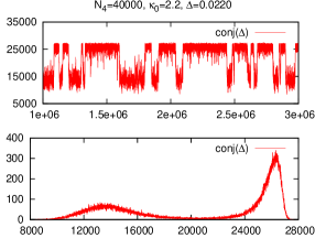
Another definition of phase transition comes from studying histograms of suitable observables. Consider the Monte Carlo time evolution of the quantity near the A-C transition, as depicted in Fig. 3 (top left). We observe that for some time fluctuates around one value, then makes a transition to another value, around which it fluctuates for a while, before flipping back to the first value again. This behaviour is characteristic of a phase transition, with the two different states corresponding to the two phases involved. The associated histogram of (Fig. 3, bottom left) shows a double-peak structure. Varying while holding fixed will change the relative heights of the two peaks. We can now fine-tune so that both peaks have the same height. This gives us another definition of the phase transition point, although often not the most practical one, since the fine-tuning can be very time-consuming. Also, there may be regions of coupling constant space or volume sizes where the flipping between the two states is not strong enough, in which case the histogram will not exhibit two peaks, but look more like a deformed Gaussian distribution.
As we move towards , all of these definitions will converge to one and the same phase transition point at infinite four-volume. However, what is important for our purposes is the observation that already for moderately large system sizes those definitions will produce values so close to each other as to be practically indistinguishable on a plot like that of Fig. 2. In order to determine the phase diagram it is therefore sufficient to fine-tune the parameters until a flipping of phases is observed. Not all observables are equally suited for this kind of analysis, because the flipping between phases can occur with different amplitudes for different observables. A good choice is usually the quantity conjugate to the coupling that needs to be fine-tuned. The form of the action (2) suggests using the quantity for the A-C transition, and for the B-C transition. The Monte Carlo time evolution and associated histogram for the latter are shown in Fig. 3 on the right (top and bottom).
It is instructive to track how the phase transition signature changes as one moves along the phase transition lines, while holding the system size fixed. Along the A-C transition we have not observed any appreciable change, although we have not investigated the immediate neighbourhood of the triple point where all three phases meet. The situation for the B-C transition is rather different. Let us start on the B-C line at the point and move in both directions along the line. As we move to the left, the jump in associated with the phase flip decreases, and around no observable signature of a phase transition remains. We conclude that the B-C transition line has an endpoint, which for is located around . Its precise location remains to be determined.
Conversely, when moving to the right from , we observe that the jump in grows rather quickly, until at we no longer observe the phase flipping, although the reason for this is very different from the situation encountered at the left endpoint. The increased size of the jump in is accompanied by a deepening of the vertical gap separating the two peaks of the histogram of . As it becomes deeper, the frequency of the phase flipping decreases significantly, until it becomes so small that no flipping is observed during the entire simulation. This indicates that the simulation becomes stuck in a metastable state and does not reach thermal equilibrium. In Fig. 2 this region is marked by a dashed line; here conventional methods are insufficient to measure the phase transition location with acceptable accuracy. We are currently investigating the use of multicanonical Monte Carlo simulations [27], which at least in principle can offer a solution to this problem.
4 How to measure the order of phase transitions
Measuring the order of phase transitions requires some care, as is illustrated by the history of dynamical triangulations. The quantum gravity model based on four-dimensional Euclidean triangulations (which lack the foliation present in CDT) has a phase transition, which initially was determined to be of second order [28, 29, 30]. However, later studies with larger systems established instead that the phase transition is of first order [31, 32].
Criteria to distinguish between first- and second-order transitions have been summarized conveniently in [33], although care should be taken in extrapolating from conventional systems, simulated on static lattices, to dynamical triangulations, where the lattice itself is dynamical. Let us begin by considering the situation of infinite system size. In this case first-order transitions are uniquely characterized by the existence of observables (first derivatives of the free energy) that are discontinuous across the transition. In addition, the size of the fluctuations relative to the average tends to zero in the infinite-volume limit, implying that the probability distribution of such an observable approaches the sum of two delta-function distributions. The displacement between the two peaks is precisely the difference between the two equilibrium values of the observable.
The probability distribution of an observable in the infinite-volume limit can be understood as arising through a limiting process of the corresponding distributions for finite volume. Their measured counterparts are histograms of the kind displayed in Fig. 3. It is sometimes stated in the literature that a double-peak structure of a histogram signals a first-order transition, but this is somewhat misleading and can even be wrong. Rather, the existence of a double-peak histogram allows one to confirm the first-order nature of a transition by considering a sequence of histograms for increasing system size. We are dealing with a first-order transition whenever the double-peak structure becomes more pronounced with increasing volume. Quantitatively, this means that the vertical gap associated with the double peak increases. By “vertical gap” we mean the difference between the peak heights (assuming they are equal) and the height of the minimum in between them. How the vertical gap changes with system size is the method of choice to confirm the first-order nature of a transition, provided one can simulate sufficiently large systems, which develop a double-peak structure. One could in principle try to use the same method to conclude that a transition is of second or higher order by measuring the vertical gap as a function of inverse system size and extrapolating to the limit of infinite volume, where it should vanish. However, because it is often difficult to measure this gap with good accuracy, showing conclusively that it really goes to zero in the limit can be problematic. Fortunately, there are better criteria at hand – involving the measurement of critical exponents – which one can use to establish that a given transition is of higher order.
One such exponent measures the shift of a transition point with system size. Recall first how this works for a conventional lattice system such as the Ising model with volume , where is the system’s dimension [34]. Considering the temperature-driven phase transition of the Ising model and using the location of the maximum of the magnetic susceptibility to define a transition point , one finds a power-law behaviour
| (3) |
for sufficiently large system size. The exponent governs the increase of the correlation length in a second-order transition as one moves towards the critical point on an infinite lattice. For first-order transitions there is no correlation length and one expects the specific scaling [33]
| (4) |
A sufficiently strong violation of therefore signals the presence of a second-order transition.
To work with the criteria (3) or (4) one needs some way of judging whether the system sizes under consideration are large enough. Given data points ordered by system size, we can make fits where the -th fit, , is made by using the restricted set of data points with labels . If the corresponding sequence of exponents is drifting, it can be an indication that the system sizes are not large enough. Obviously, this method is only useful when one has sufficiently many data points.
Another quantity of interest is the so-called Binder cumulant associated with an observable , which may be defined as [33]
| (5) |
and is always nonpositive. Considering as a function of the couplings, its local minima are at transition points, where the fluctuations are largest. We can measure these minima for different system sizes and by extrapolation determine . This quantity is zero when the probability distribution of approaches a delta function around an expectation value in the infinite-volume limit, as is expected at a second-order transition. On the other hand, many aspects of first-order transitions are described well by approximating the histogram of the observable with a superposition of two distributions centred at the expectation values and in the two phases. Again, if these distributions approach delta functions in the infinite-volume limit, the minimum of will be given by
| (6) |
which is obtained for a value of the coupling constants where the relative strength of the delta functions at and is given by and respectively. We conclude that a sufficiently strong deviation of from zero signals a first-order phase transition. Using the value of the Binder cumulant to make the case for a second-order transition is more difficult, because a weak first-order transition may show a convergence to a value close to zero.
There are other methods, involving the measurement of other critical exponents, which can help to determine the order of a phase transition, but their translation to CDT quantum gravity leads to ambiguities. We will therefore proceed by applying the methods described above to the A-C and B-C transitions found in the CDT system. The third transition (A-B) is currently of minor interest, since it bounds two phases that most likely have no relevance for continuum physics.
4.1 The order of the A-C transition
The simulations for the analysis of the A-C transition were run at , with system sizes ranging from to . The data presented in the following are the results of simulations where the number of sweeps was approximately , with one sweep representing one million attempted Monte Carlo moves.
Our simulations suffer from a slow convergence of observables, which means that the standard error algorithms produce error values which significantly underestimate the true uncertainties of the measurements. In all our measurements we have attempted to obtain more realistic error values by systematically studying the convergence of observables. Given a set of data samples at Monte Carlo times , we can define a time-dependent average by including only those data samples for which . We then plot this quantity as a function of and try to extract reasonable error values. This method introduces a degree of subjectivity, but in our opinion produces more realistic error estimates.
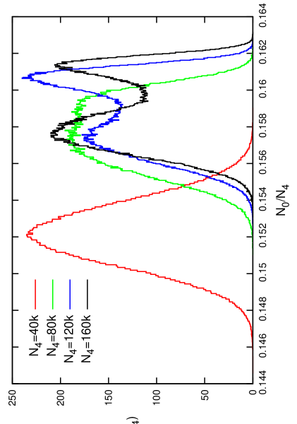
We first perform a histogram analysis. Fig. 4 shows the histograms for the observable (more precisely, the rescaled quantity ) at four different system sizes. The histogram at assumes an approximate Gaussian shape, which gets distorted at , with a double peak starting to emerge at , which becomes more pronounced at . For the two larger volumes, the vertical gap associated with the double-peak clearly increases, while the mutual distance of the peaks stays approximately the same. This behaviour is a clear signature of a first-order transition. The emergence of the double-peak shape seems to occur somewhere between and . This may be compared with the analysis performed in the context of four-dimensional Euclidean dynamical triangulations, where the double peak emerged between and [31]. The more rigid structure imposed on the triangulations by the causality conditions of CDT may be responsible for the shift of the appearance of the first-order signal to somewhat larger volumes.
Let us try to find additional evidence for the first-order nature of the A-C transition by first measuring the shift exponent defined in eq. (4). For sufficiently large system sizes we expect a power-law behaviour
| (7) |
where denotes the transition point at system size and is a proportionality factor.
We have already mentioned that the notion of a transition point is ambiguous for finite system sizes. For our present purposes, we define as the location of the maximum of the susceptibility . To measure this maximum we use an extrapolation method due to Ferrenberg and Swendsen [35], also known as histogram method [34].
The best fit using all data points gives , with a reduced chi-squared of . Unfortunately, the three-parameter fit (7) is not very stable when removing the points with the lowest values of . Taking this into account, it becomes clear that the error bar of 0.02 significantly underestimates the error associated with the determination of from the data. It indicates the presence of subleading terms which for the volume range studied interfere with the pure power-law behaviour of (7). Consequently, the strongest conclusion we can draw from using this method is that the measured is compatible with the value characteristic of a first-order transition.
As an additional cross-check we have made another three-parameter fit to the generic functional form of a large- expansion of , valid at a first-order transition [33], namely,
| (8) |
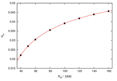
Fig. 5 shows the measured data points and the best fit, based on the expansion (8). The errors associated with individual data points are too small to be visualized in a sensible way. The quality of this fit is comparable with that obtained from fitting to the power law (7). The contribution from the -term is subdominant to that from the -term, as should be. To summarize, we can say with confidence that the shift data are fully compatible with a first-order transition. However, it is also clear that if one wanted to go beyond this statement and nail down the value of the critical exponent with better precision, one would need to consider larger system sizes.
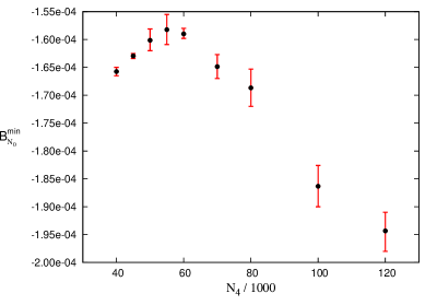
Our next and final step in analyzing the A-C transition will be to consider the Binder cumulant for ,
| (9) |
which has a local minimum at the A-C phase transition. Like in the case of the shift exponent , we use the histogram method to determine this minimum. In Fig. 6 we have plotted as a function of system size. The error bars are much larger than for the measurement of the shift exponent, where we measured the location of the susceptibility maximum, and not the maximum value itself. The plot shows clearly that moves away from zero as one goes to large system sizes, reconfirming the first-order nature of the transition.
By contrast, when going to smaller volumes one finds a different behaviour, where increases before reaching a local maximum. Evidently, for these small volumes the system lies outside the scaling region, where quantities like are expected to behave according to a power law. Looking at the plot, a rough estimate of the onset of the scaling region seems to be around or above . Comparing with Fig. 4, this may be correlated with the observed emergence of the double-peak structure in the histograms.
4.2 The order of the B-C transition
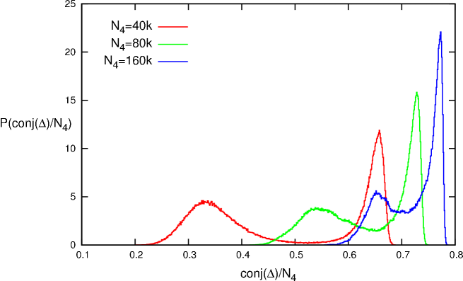
Continuing our investigation of the order of phase transitions in CDT quantum gravity, we now turn to the B-C transition. In this case, we have fixed the inverse gravitational coupling to and analysed the system at sizes between and . The number of sweeps used was approximately , with one sweep again corresponding to one million attempted Monte Carlo moves. Fig. 7 shows the histograms of the quantity for three different system sizes. The situation differs from that of the A-C transition in that we observe a double-peak structure for all four-volumes. The peaks are most pronounced for smaller volume and appear to be merging when the volume is increased. The plot shows that their mutual distance decreases, roughly like . This is a first indication that the B-C transition may not be a first-order transition.111Since we have not performed a time-consuming fine-tuning of to obtain peaks of equal height, we have not been able to extract a reliable estimate of their vertical gap (relative height of peaks w.r.t. minimum in between peaks, as defined earlier in Sec. 4).
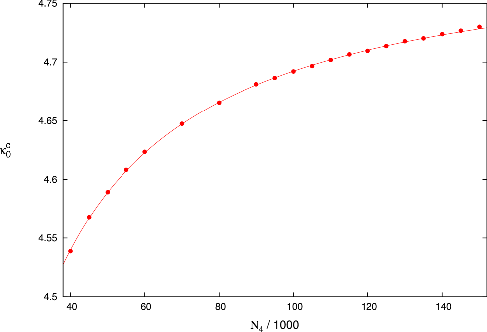
We proceed by measuring the shift exponent for . Analogous to what we did for the A-C transition, we will use the formula
| (10) |
where is defined as the location of the maximum of the susceptibility . Data points and best fit are displayed in Fig. 8. We have not included any error bars because they turned out to be too small. The best fit through all data points yields . To judge whether our range of system sizes lies inside the scaling region we have again performed a sequence of fits by successively removing the data points with the lowest four-volume. The corresponding values for are , , and , where the last fit was done with all but five data points removed. Again the error bars are based on making cuts in the sampled data as described above when discussing the A-C transition. The sequence suggests that the data point with the lowest four-volume lies outside the scaling region. Removing it from the fit we get
| (11) |
This result makes a strong case for a second-order transition, since the prediction for a first-order transition is clearly violated.
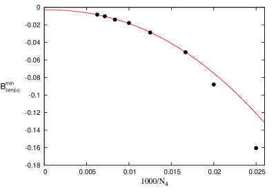
Let us finally consider how the minimum of the Binder cumulant of definition (5), with , depends on the system size. In Fig. 9 we show as a function of inverse system size. The errors turned out to be much smaller than for the corresponding measurements at the A-C transition, with error magnitude approximately equal to the radius of the dots in the plot. Inside the scaling region the minimum of the Binder cumulant is expected to behave like a power-law function. To determine whether our data points lie inside this scaling region, we have again performed a sequence of fits by successively removing the data points with the lowest four-volume. We have found that the data points at and both lie outside the scaling region. The curve displayed in Fig. 9 corresponds to the fit with those two points removed.
| Observable | |
|---|---|
Table 1 collects the results of measuring for five different observables . All of these observables exhibit a phase flipping at the transition, with associated double-peak histograms. The interpolation to is made by assuming that the quantities for sufficiently large volumes have a scaling behaviour like in eqs. (7) and (10), namely,
| (12) |
with -dependent exponents and coefficients . If we had to rely on the Binder cumulant measurements alone to determine the order of the B-C transition, we would encounter the already mentioned problem of how to distinguish between a second-order transition and a first-order transition where converges to a value close to zero. In the case at hand, in addition to the evidence already presented in favour of a second-order transition, the size and quality of the measurement errors for the minimum of the Binder cumulants are such that we can conclude with confidence that the results displayed in Table 1 are certainly consistent with a limiting value of zero for . This would be true even if the errors overestimated the true uncertainties by a factor of two, say.
5 Discussion and outlook
We set out with the goal to determine the order of the two physically relevant phase transitions in CDT quantum gravity. For conventional systems on static lattices, describing physics on a fixed background geometry, the methods for doing so are well established. It is not clear a priori whether all of them are applicable for systems based on dynamical lattices, such as CDT, which reflect the dynamical character of the quantum-gravitational, geometric degrees of freedom they aim to describe. Evidence that standard methods can be adapted rather straightforwardly to systems of dynamical geometry comes from Euclidean dynamically triangulated (DT) systems. This has been demonstrated for two-dimensional Euclidean quantum gravity (coupled to matter), where extensive computer simulations [36] are in agreement with Liouville quantum gravity, which can be solved analytically. It is also true in four-dimensional DT. Although this model does not appear to describe four-dimensional quantum gravity, it does exhibit a well-defined scaling behaviour in the so-called branched-polymer phase and finite-size scaling works very well [30].
However, since causal dynamical triangulations differ from their purely Euclidean counterparts both in their set-up and (hopefully) the continuum physics they describe, we decided to not take the validity of these methods for granted. Rather, we used several independent criteria for determining the transition orders, and checked whether the results were mutually consistent.
Our analysis consisted of three parts: the histogram analysis, the measurement of the shift exponent and the analysis of Binder cumulants. The histogram analysis was sufficient to confirm the first-order nature of the A-C transition. It probes the definition of a first-order transition in a direct way and is therefore the method of choice to confirm the first-order nature of a transition. Measurements of the Binder cumulants also pointed rather unambiguously to a first-order transition. The absolute values of the minima were increasing for increasing volume , contrary to what one would expect for a second-order transition. Measurements of the shift exponent, which governs the dependence of transition points on the system size, were less conclusive. The results were compatible with , valid at a first-order transition. However, since the stability of the curve fits under successive removal of data points with small volume was not particularly good, we did not succeed in determining the exponent convincingly from the data, but only in establishing its consistency with the first-order value.
The corresponding analysis of the B-C transition gave a very different picture. The histogram analysis showed a double-peak structure, but without the characteristic features of a first-order transition. The distance between the two peaks diminished with increasing , indicating a higher-order transition. This was corroborated by measuring the shift exponent, whose value entails a strong violation of the prediction for a first-order transition. In addition, the results of the Binder cumulant analysis were also clearly consistent with the presence of a second-order B-C transition, as announced previously in [16].
In summary, we have found strong evidence that in CDT quantum gravity the A-C transition line is first order, while the B-C transition line is second order. The latter result is both remarkable and attractive. It opens the door to studying critical phenomena in CDT and to defining a continuum limit for vanishing lattice spacing (UV cutoff). A discussion of the effective gravitational coupling constant, and its dependence on the bare couplings of the model – inside phase C – was initiated in [15]. In view of the results presented here, a future task will be to extend this analysis by studying the flow of this coupling constant when approaching the second-order B-C phase transition line. Apart from the intrinsic interest in understanding the behaviour of quantum-gravitational observables in this limit, which appears to be associated with probing (sub-)Planckian physics, this may enable one to make a more explicit connection with the asymptotic safety scenario, as outlined recently in [13], as well as anisotropic gravity models of Hořava-Lifshitz type.
To make this connection more concrete, let us consider a potential application of our analysis, based on the presence of a second-order transition. As shown in [14, 17], well inside phase C the time extent of the universe scales like , and the three-volume of a generic spatial slice at time like . By contrast, in phase this time extent essentially vanishes, since all three-volume is located at a single spatial slice. Approaching the B-C transition line from inside phase C, we observe that , measured in lattice time steps, decreases, at least in the region where detailed measurements are available. Its precise behaviour still needs to be determined, but it is natural to conjecture a behaviour of the form
| (13) |
at the pseudo-critical point . Combining this with the scaling (10) of the coupling , we obtain
| (14) |
implying that the time extent scales anomalously. Interestingly, such an anomalous scaling of time relative to space in the ultraviolet is also a key feature of Hořava-Lifshitz gravities [25]. Following this line of reasoning further, one could imagine that both and depended on , in this way potentially allowing for both anisotropic and isotropic UV completions, depending on where the B-C phase transition line is approached.
Acknowledgements.
JA thanks the ITP and the Department of Physics and Astronomy of Utrecht University, as well as the Perimeter Institute for hospitality and financial support. He also acknowledges financial support of the Danish Research Council under the grant ”Quantum gravity and the role of black holes”. JJ acknowledges partial support through the Polish Ministry of Science grants N N202 229137 (2009-2012) and 182/N-QGG/2008/0. SJ would like to thank Prof. G.T. Barkema for fruitful discussions and valuable advice concerning the numerical aspects of this work. RL acknowledges support by the Netherlands Organisation for Scientific Research (NWO) under their VICI program. The contributions by SJ and RL are part of the research programme of the Foundation for Fundamental Research on Matter (FOM), financially supported by NWO. This research was supported by Perimeter Institute for Theoretical Physics. Research at Perimeter Institute is supported by the Government of Canada through Industry Canada and by the Province of Ontario through the Ministry of Research and Innovation.
References
- [1] J.F. Donoghue, Introduction to the effective field theory description of gravity, in Proceedings of the Advanced School on Effective Theories, Almunecar, Spain, eds. F. Cornet and M.J. Hererro, World Scientific (1997) [gr-qc/9512024].
- [2] C.P. Burgess, Quantum gravity in everyday life: General relativity as an effective field theory, Living Rev. Rel. 7 (2004) [gr-qc/0311082].
- [3] T. Rothman and S. Boughn, Can gravitons be detected?, Found. Phys. 36 (2006) 1801-1825 [gr-qc/0601043].
- [4] S. Weinberg, Ultraviolet divergences in quantum theories of gravitation, in General relativity: Einstein centenary survey, eds. S.W. Hawking and W. Israel, Cambridge University Press, Cambridge, UK (1979) 790-831.
-
[5]
S. Christensen and M. Duff, Quantum gravity in 2+
dimensions,
Phys. Lett. B 79 (1978) 213-216;
R. Gastmans, R. Kallosh and C. Truffin, Quantum gravity near two dimensions, Nucl. Phys. B 133 (1978) 417-434. -
[6]
H. Kawai and M. Ninomiya,
Renormalization group and quantum gravity,
Nucl. Phys. B 336 (1990) 115;
H. Kawai, Y. Kitazawa and M. Ninomiya, Scaling exponents in quantum gravity near two-dimensions, Nucl. Phys. B 393 (1993) 280-300 [hep-th/9206081];
Ultraviolet stable fixed point and scaling relations in (2+)-dimensional quantum gravity, Nucl. Phys. B 404 (1993) 684-716 [hep-th/9303123];
Renormalizability of quantum gravity near two dimensions, Nucl. Phys. B 467 (1996) 313-331 [hep-th/9511217];
T. Aida, Y. Kitazawa, H. Kawai and M. Ninomiya, Conformal invariance and renormalization group in quantum gravity near two-dimensions, Nucl. Phys. B 427 (1994) 158-180 [hep-th/9404171]. - [7] M. Niedermaier, The asymptotic safety scenario in quantum gravity: an introduction, Class. Quantum Grav. 24 (2007) R171-R230.
- [8] M. Reuter, Nonperturbative evolution equation for quantum gravity, Phys. Rev. D 57 (1998) 971-985 [hep-th/9605030].
-
[9]
D. Benedetti, P.F. Machado and F. Saueressig,
Asymptotic safety in higher-derivative gravity,
Mod. Phys. Lett. A 24 (2009) 2233 [arXiv:0901.2984, hep-th];
A. Codello, R. Percacci and C. Rahmede, Investigating the ultraviolet properties of gravity with a Wilsonian renormalization group equation, Annals Phys. 324 (2009) 414 [arXiv:0805.2909, hep-th];
M. Reuter and F. Saueressig, Functional renormalization group equations, asymptotic safety, and Quantum Einstein Gravity [arXiv:0708.1317, hep-th].
M. Niedermaier and M. Reuter, The asymptotic safety scenario in quantum gravity, Living Rev. Rel. 9 (2006) 5;
H.W. Hamber and R.M. Williams, Nonlocal effective gravitational field equations and the running of Newton’s G, Phys. Rev. D 72 (2005) 044026 [hep-th/0507017];
D.F. Litim, Fixed points of quantum gravity, Phys. Rev. Lett. 92 (2004) 201301 [hep-th/0312114]. - [10] M. Reuter and F. Saueressig, Quantum Einstein gravity [arXiv:1202.2274, hep-th].
- [11] R. Loll, Discrete approaches to quantum gravity in four dimensions, Living Rev. Rel. 1 [gr-qc/9805049].
-
[12]
J. Ambjørn, A. Görlich, J. Jurkiewicz and R. Loll,
CDT - an entropic theory of quantum gravity [arXiv:1007.2560, hep-th];
J. Ambjørn, J. Jurkiewicz and R. Loll, Causal dynamical triangulations and the quest for quantum gravity, in Foundations of space and time, eds. G.F.R. Ellis, J. Murugan and A. Weltman, Cambridge University Press, Cambridge, UK (2012), to appear [arXiv:1004.0352, hep-th];
Quantum gravity as sum over spacetimes, Lect. Notes Phys. 807 (2010) 59-124 [arXiv:0906.3947, gr-qc];
The universe from scratch, Contemp. Phys. 47 (2006) 103-117 [hep-th/0509010];
Quantum gravity, or, The art of building spacetime, in Approaches to quantum gravity, ed. D. Oriti, Cambridge University Press, Cambridge, UK (2009) 341-359 [hep-th/0604212]. - [13] J. Ambjørn, A. Görlich, J. Jurkiewicz and R. Loll, Nonperturbative quantum gravity, Phys. Rep. (2012), to appear [arXiv:1203.3591, hep-th].
- [14] J. Ambjørn, J. Jurkiewicz and R. Loll, Emergence of a 4D world from causal quantum gravity, Phys. Rev. Lett. 93 (2004) 131301 [hep-th/0404156].
-
[15]
J. Ambjørn, A. Görlich, J. Jurkiewicz and R. Loll,
The nonperturbative quantum de Sitter universe,
Phys. Rev. D 78 (2008) 063544 [arXiv:0807.4481, hep-th];
J. Ambjørn, J. Jurkiewicz and R. Loll, Semiclassical universe from first principles, Phys. Lett. B 607 (2005) 205-213 [hep-th/0411152]. - [16] J. Ambjørn, S. Jordan, J. Jurkiewicz and R. Loll, A second-order phase transition in causal dynamical triangulations, Phys. Rev. Lett. 107 (2011) 211303 [arXiv:1108.3932, hep-th].
- [17] J. Ambjørn, J. Jurkiewicz and R. Loll, Reconstructing the universe, Phys. Rev. D 72 (2005) 064014 [hep-th/0505154].
-
[18]
J. Ambjørn, J. Jurkiewicz and R. Loll,
A non-perturbative Lorentzian path integral for gravity,
Phys. Rev. Lett. 85 (2000) 924 [hep-th/0002050];
Dynamically triangulating Lorentzian quantum gravity, Nucl. Phys. B 610 (2001) 347-382 [hep-th/0105267]. - [19] J. Ambjørn, A. Görlich, J. Jurkiewicz and R. Loll, Planckian birth of the quantum de Sitter universe, Phys. Rev. Lett. 100 (2008) 091304 [arXiv:0712.2485, hep-th].
- [20] T. Regge: General relativity without coordinates, Nuovo Cim. 19 (1961) 558.
- [21] J. Ambjørn and R. Loll: Non-perturbative Lorentzian quantum gravity, causality and topology change, Nucl. Phys. B 536 (1998) 407-434 [hep-th/9805108].
-
[22]
J. Ambjørn, J. Jurkiewicz and R. Loll,
Renormalization of 3-d quantum gravity from matrix models,
Phys. Lett. B 581 (2004) 255-262 [hep-th/0307263];
J. Ambjørn, J. Jurkiewicz, R. Loll and G. Vernizzi, Lorentzian 3-D gravity with wormholes via matrix models, JHEP 0109 (2001) 022 [hep-th/0106082]. - [23] D. Benedetti, R. Loll and F. Zamponi: (2+1)-dimensional quantum gravity as the continuum limit of causal dynamical triangulations, Phys. Rev. D 76 (2007) 104022 [arXiv:0704.3214, hep-th].
- [24] J. Ambjørn, A. Görlich, S. Jordan, J. Jurkiewicz and R. Loll, CDT meets Hořava-Lifshitz gravity, Phys. Lett. B 690 (2010) 413-419 [arXiv:1002.3298, hep-th].
-
[25]
P. Hořava,
Quantum gravity at a Lifshitz point,
Phys. Rev. D 79 (2009) 084008 [arXiv:0901.3775, hep-th];
P. Hořava and C.M. Melby-Thompson, General covariance in quantum gravity at a Lifshitz point, Phys. Rev. D 82 (2010) 064027 [arXiv:1007.2410, hep-th];
C. Anderson, S. Carlip, J.H. Cooperman, P. Hořava, R. Kommu and P.R. Zulkowski, Quantizing Hořava-Lifshitz gravity via causal dynamical triangulations, Phys. Rev. D 85 (2012) 044027 (Phys. Rev. D 85 (2012) 049904) [arXiv:1111.6634, hep-th]. - [26] P. Hořava, General covariance in gravity at a Lifshitz point, Class. Quant. Grav. 28 (2011) 114012 [arXiv:1101.1081, hep-th].
- [27] B.A. Berg, Introduction to multicanonical Monte Carlo simulations, Fields Inst. Commun. 26 (2000) 1 [cond-mat/9909236].
- [28] J. Ambjørn and J. Jurkiewicz, Four-dimensional simplicial quantum gravity, Phys. Lett. B 278 (1992) 42-50.
- [29] S. Catterall, J.B. Kogut and R. Renken, Phase structure of four-dimensional simplicial quantum gravity, Phys. Lett. B 328 (1994) 277-283 [hep-lat/9401026].
- [30] J. Ambjørn and J. Jurkiewicz, Scaling in four-dimensional quantum gravity, Nucl. Phys. B 451 (1995) 643-676 [hep-th/9503006].
- [31] P. Bialas, Z. Burda, A. Krzywicki and B. Petersson, Focusing on the fixed point of 4-D simplicial gravity, Nucl. Phys. B 472 (1996) 293-308 [hep-lat/9601024].
- [32] B.V. de Bakker, Further evidence that the transition of 4D dynamical triangulation is 1st order, Phys. Lett. B 389 (1996) 238-242 [hep-lat/9603024]
- [33] H. Meyer-Ortmanns, Phase transitions in quantum chromodynamics, Rev. Mod. Phys. 68 (1996) 473-598 [hep-lat/9608098].
- [34] M.E.J. Newman and G.T. Barkema Monte Carlo methods in statistical physics, Oxford University Press, Oxford, UK (2002).
- [35] A.M. Ferrenberg and R.H. Swendsen, New Monte Carlo technique for studying phase transitions, Phys. Rev. Lett. 61 (1988) 2635-2638.
-
[36]
J. Ambjørn and K.N. Anagnostopoulos,
Quantum geometry of 2D gravity coupled to unitary matter,
Nucl. Phys. B 497 (1997) 445-478 [hep-lat/9701006];
J. Ambjørn, J. Jurkiewicz and Y. Watabiki, On the fractal structure of two-dimensional quantum gravity, Nucl. Phys. B 454 (1995) 313-342 [hep-lat/9507014].