Low energy electron/recoil discrimination for directional Dark Matter detection

Abstract

Directional detection is a promising Dark Matter search strategy. Even though it could accommodate to a sizeable background contamination, electron/recoil discrimination remains a key and challenging issue as for direction-insensitive detectors. The measurement of the 3D track may be used to discriminate electrons from nuclear recoils. While a high rejection power is expected above 20 keV ionization, a dedicated data analysis is needed at low energy. After identifying discriminant observables, a multivariate analysis, namely a Boosted Decision Tree, is proposed, enabling an efficient event tagging for Dark Matter search. We show that it allows us to optimize rejection while keeping a rather high efficiency which is compulsory for rare event search.With respect to a sequential analysis, the rejection is about $\sim 20$ times higher with a multivariate analysis, for the same Dark Matter exclusion limit.

Directional detection of Dark Matter has been first proposed as a powerful tool to identify genuine WIMP events as such [1]. Since then, the contribution of directional detection to the field of Dark Matter has been adressed through a wealth of studies [2, 3, 4, 5, 6, 7, 8, 9, 10, 11, 12, 13, 14, 15, 16, 17, 18, 19, 20, 21]. In particular, it has been shown that even a low exposure directional detector (30 kg.year) could lead to a high significance discovery of galactic Dark Matter [4, 6, 19]. For neutralino Dark Matter, most MSSM configurations with a neutralino lighter than 200 $\rm GeV/c^{2}$ would lead to a significance greater than 3$\sigma$ (90% CL) in a 30 kg.year CF4 directional detector [2].
There is a worldwide effort toward the development of a large directional detector [22, 23, 24, 25, 26, 27], most projects being low pressure Time Projection Chambers (TPC). All current projects face common challenges, some being specific to directional detection, some being shared with direction-insensitive strategy [28]. In particular, zero background is often referred to as the ultimate goal for the next generation of direct detection experiments in deep underground laboratories. Even though directional detection could accommodate to a sizeable background contamination [6, 7], owing to the large intrinsic difference between the WIMP-induced and background-induced spectra, electron/recoil discrimination remains a key and challenging issue as for direction-insensitive detectors. For the latter, electron/recoil discrimination may be achieved thanks to a double detection of the energy : heat/ionization [29, 30], scintillation/ionization [31, 32] or heat/scintillation [33]. As far as directional detection is concerned, only the ionization energy is measured and the discrimination cannot rely on the measurement of the energy deposit only. However, as early suggested in [34, 35], the information on the 3D track may be used to discriminate electron and nuclear recoils. A recent study [36] has shown the possibility to achieve 3D reconstruction in the case of the MIMAC project [26]. In particular, the vertex (X, Y and Z) of the elastic scatterring interaction can be retrieved, thus enabling a fiducialization of the detector and hence reducing the background contamination from surface events. However an e/recoil discrimination method would be a powerful way to further reduce background contamination.
In this paper, we propose a new method to discriminate electron from nuclear recoils. It is based on discriminant observables related to track topology. High rejection power is expected at high energy (above 50 keV recoil) but low energy discrimination requires a careful data analysis and a multivariate analysis, namely a Boosted Decision Tree, is proposed to optimize rejection while keeping a rather high efficiency. This event tagging based on a Boosted Decision Tree method is of general interest for Dark Matter search and could be adapted for various e/recoil discrimination strategies.

The paper is organised as follows, we first choose discriminant observables and study their correlations (sec. 1). Then, an electron/recoil discrimination is proposed within the framework of a sequential analysis (sec. 2). In section 3, we introduce a Boosted Decision Tree method, used to tag events either as electron or nuclear recoil. We conclude in sec. 4 by showing the consequences in terms of Dark Matter search.

1 Discriminant observables

In the following, we present the MIMAC track reconstruction strategy (sec. 1.1), discuss a full simulation of tracks in the MIMAC detector (sec. 1.2). Then, we choose discriminant observables (sec. 1.3) and study their correlations (sec. 1.4).

1.1 MIMAC track measurement strategy

The MIMAC detector is a project dedicated to directional Dark Matter search [26]. It is a matrix design of elementary $CF_{4}$ TPC operated at low pressure (50 mbar). The primary electron-ion pairs produced by a nuclear recoil in one chamber of the matrix are detected by drifting the primary electrons to the grid of a bulk Micromegas [37, 38] and producing the avalanche in a very thin gap (128 or 256 $\mu$m). The electrons move towards the grid in the drift space and are projected on the pixelized anode thus allowing to get information on the X and Y coordinates. A bulk Micromegas [37, 38] with a 10.8 by 10.8 cm² active area, segmented in pixels with an effective pitch of 424 $\mu$m is used as 2D readout. In order to reconstruct the third dimension of the recoil, the Z coordinate i.e. along the drift axis, a self-triggered electronics has been developed [39, 40, 41]. The ionization energy measurement is done by using a charge integrator connected to the grid sampled at a frequency of 50 MHz. Then, to recover the kinetic energy of the recoiling nucleus, one has to know accurately the value of the Ionization Quenching Factor (IQF) [42]. With such a measurement, the X and Y coordinates are measured on the anode, while the Z coordinate is retrieved from the 50 MHz sampling of the anode. Hence, the track is 3D reconstructed, providing the electron drift velocity is known [43, 44]. A dedicated data analysis method [36] allows us to retrieve, for each track, the initial recoil direction ($\theta,\phi$) together with the vertex (X, Y and Z) of the WIMP elastic scatterring interaction. In particular, the latter enables a detector fiducialization which reduces the background contamination from surface events. However an e/recoil discrimination method would be a powerful way to further reduce background contamination.

1.2 Track simulation in MIMAC

We use the same simulation software as in [36]. For the reader’s convenience, we recall the main points hereafter, noticing that a comprehensive discussion on systematics of track measurement may be found in [36]. As a matter of fact, a realistic track simulation in a low pressure TPC should include all processes and systematics: generation of electron or nuclear recoils, primary electron generation, electron drift properties, readout and trigger strategy. The simulation scheme is the following :

• Electron and nuclear recoils are simulated respectively with the Geant4 software [45] and the SRIM software [46]. The kinetic energy spectrum is chosen as flat, between 0 and 50 keV for electrons and 1 and 120 keV for Fluorine recoils. All events are randomly generated within the whole detector volume ($10.8\times 10.8\times 25\ {\rm cm}^{3}$) and with an isotropic distribution.

• Electron/ion pair generation is accounted for. For a given energy loss, primary electrons are randomly generated between two collision points.

• Electron drift properties are estimated with the Magboltz software [44], The drift velocity ($v_{d}$) and both the transversal and longitudinal diffusion ($D_{l}$ and $D_{t}$) are accounted for. The gas mixture is 70% CF₄ and 30% de CHF₃ at 50 mbar. For a 100 V/cm drift field, we found : $v_{d}=21.4$ $\mu$m/ns, $D_{l}=278.4\ \mu{\rm m/\sqrt{cm}}$ and $D_{t}=246.0\ \mu{\rm m/\sqrt{cm}}$.

• The Micromegas is simulated with a 100% transparency and a gain of $\sim$ 10³, ensuring that each row of pixels is sensitive to the unique electron.

• Eventually, the track enveloppe formed by primary electrons generated along the track is then sampled with the MIMAC strategy. The pixelized anode is composed of 256 channels in X and Y, with an effective width of 424 $\mu$m. Each pixel is connected either with a X or Y channel. For a given event, an X-Y coincidence is thus required to locate the position on the anode. The Z coordinate is then reconstructed thanks to the 50 MHz sampling of the anode. Hence, each track is characterized by $N_{c}$ time coincidences.

As the simulated tracks must contain all systematics associated to data tracks, we emphasize that the MIMAC readout and trigger strategy are accounted, which is a key point of the simulation scheme. This allows us to include time sampling, pitch size, thresholds, missing coincidences and experimental limitations.. This simulation software provides us with a realistic set of simulated tracks, with various energies, drift sizes or gas properties.
A loose selection is imposed on simulated events : all events must have at least one coincidence $N_{c}>1$ and be fully enclosed within the detector, i.e. no border strips fired.

1.3 Defining discriminant observables

For a given energy, the track topology is expected to depend on the recoiling particle (electron or nucleus) and discriminant observables should be identified to evaluate the expected rejection power and efficiency. Figure 1 presents the 2D projections, in the (X,Z) plane, of simulated tracks : a 100 keV Fluorine (left) and a 10 keV electrons (right). Both tracks are simulated with a common inital vertex (1 cm from the anode and in its center) and a common direction (perpendicular to the anode and going to the cathode). It is straightforward to notice that the topology of the tracks are very different. First, the length of the electron track is much longer than the one of the nuclear recoil, even with a kinetic energy ten time smaller. Hence, the first idea is to use the track length as a discriminant observable, since for a given kinetic energy the range of electrons is expected to be much larger than the one of nuclear recoils. However, instead of using the projected range as an estimation of the track length, we define the curve length ($L_{c}$) as :

$$L_{c}=\sum_{i=1}^{N_{c}-1}\sqrt{(X_{i+1}-X_{i})^{2}+(Y_{i+1}-Y_{i})^{2}+(Z_{i+1}-Z_{i})^{2}}$$ (1)

with $N_{c}$ the number of coincidences, ($X_{i},Y_{i},Z_{i}$) the barycentre location for each coincidence. $L_{c}$ is thus the sum of segments linking each consecutive barycentre. The interest of this observable is the fact that it is strongly correlated to the range but it does also include the effect of small angular deflections along the track (see fig. 1). This enhances the difference between electrons and nuclear recoils and reduces the RMS of the range distribution to get a better discrimination. We highlight the fact that the curve length definition also includes electron longitudinal diffusion effect. 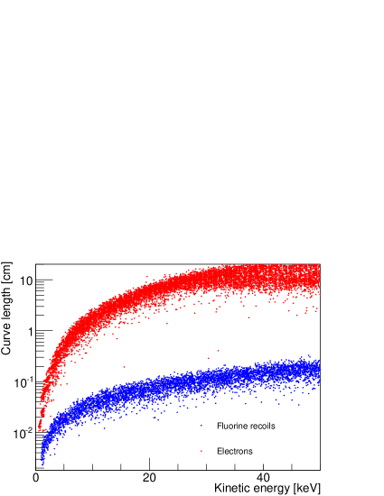For instance, it is about 1 mm for a 16 cm drift. Figure 2 presents the curve length for simulated electrons (red) and nuclear recoils (blue) as a function of the kinetic energy. This result has been obtained from raw tracks from the simulation, before accounting for electron drift properties and detector sampling. It must hence be taken as the best discrimination that can be obtained from this observable (see fig. 3 to estimate the effect of drift and sampling). The ratio between the average electron curve length and the nuclear recoil one ranges between 1 and 2 orders of magnitude, depending on the kinetic energy. Note that above 30 keV, the electron distribution is getting broader due to the size of the detector ($10.8\times 10.8\times 25\ {\rm cm}^{3}$).

Figure 1: 2D projections, in the (X,Z) plane, of simulated tracks : a 100 keV Fluorine (left) and a 10 keV electrons (right). See text for details.

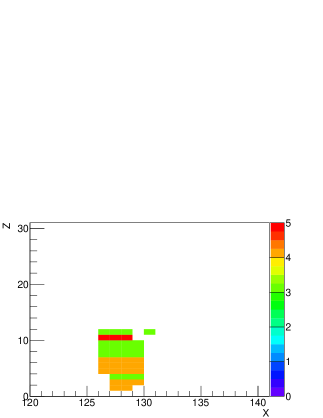
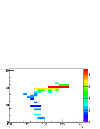
The second observable is related to the track angular deviations. Indeed, as can be noticed on fig. 1, a nuclear recoil track seem to be much more compact, with less angular deflections than an electron one. The observable includes the number of kinks encountered by the recoiling particle, and their magnitude. We define the Normalized Integrated Straggling (NIS) as :

$${\rm NIS}=\frac{1}{E_{ion}}\sum_{i=1}^{N_{c}-2}\Delta\theta_{i}$$ (2)

It is the sum of angular deviation ($\Delta\theta_{i}$) between each consecutive barycentre ($X_{i},Y_{i},Z_{i}$), normalized by the total ionization energy. The ionization energy is taken in arbitrary units in the definition as it depends on the calibration in real life experiments.

Of course, other observables could be deduced from such 3D tracks, but they are all correlated with the one we have chosen and with a smaller discrimination power. For instance the projected range is closely related to the curve length. The fraction of spatial coincidences ($N_{c}/\Delta t_{e}$), close to 1 for nuclear recoils and ranging between 0 and 1 for electrons, is also correlated with the NIS and the curve length. We converge to 3 observables ($E_{ion},L_{c}$ and NIS) to discriminate electrons from nuclear recoils.

Figure 2: Curve length as a function of the kinetic energy, for electrons (red) and Fluorine recoils (blue). Result obtained from raw tracks from the simulation, before accounting for electron drift properties and detector sampling.

Figure 3: Marginalised distributions (diagonal) and 2D correlations (off-diagonal) plots of the 3 observables ($E_{ion}$, $L_{c}$ and NIS). Electrons (red crosses) and Fluorine recoils (blue circles) are presented.

1.4 Distribution and correlation of discriminant observables

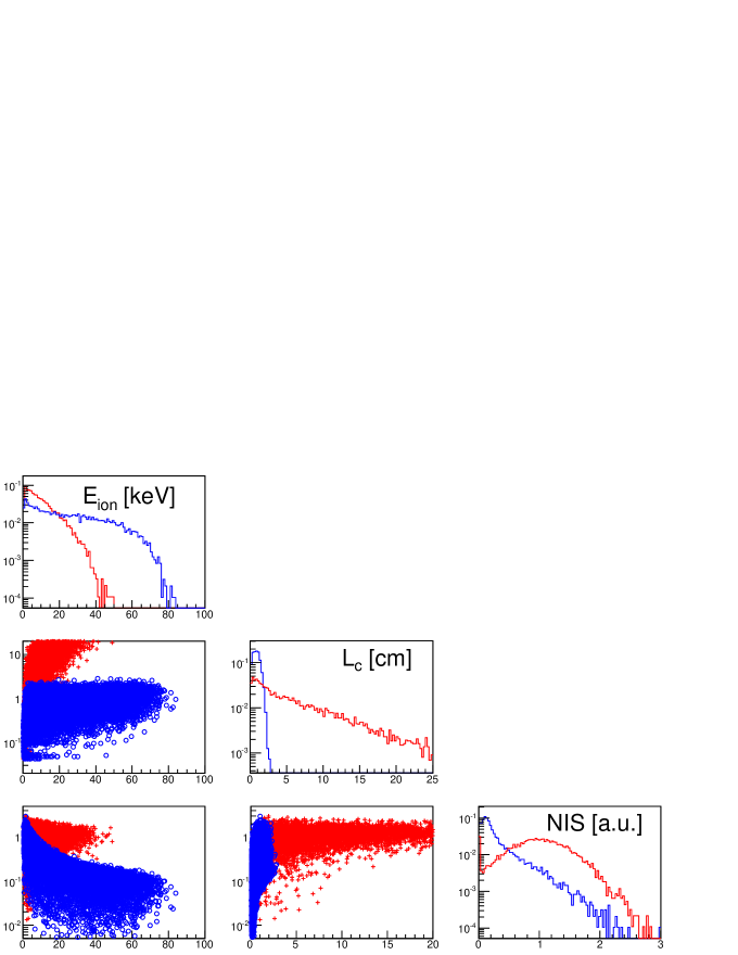
In the following, we study the distributions of these observables and their correlations in order to define the selections used in the following. Figure 3 presents the marginalised distributions (diagonal) and 2D correlations (off-diagonal) plots of the 3 observables. Electrons (red) and nuclear recoils (blue) are presented.

Ionization energy
First, concerning the ionization energy (first row, first column), it is worth emphasizing that the simulated recoil energy spectrum is chosen as flat, between 0 and 50 keV for electrons and between 1 and 120 keV for Fluorine recoils. The distribution of ionization energy of Fluorine recoils is steadily decreasing with an end point close to 80 keV. This is due to the ionization quenching effect. Indeed, at 120 keV the ionization quenching factor, from SRIM simulation, is of the order of 65%. Concerning electron recoils, the ionization energy distribution is also decreasing due to a finite-size effect. Indeed, at high energy the typical electron track length, whatever the definition, reaches the size of the detector. As the events are generated randomly within the detector volume, the effect appears also at lower energy. Note that there is of course no finite-size effect for nuclear recoils as the track length are very small, compared with the size of the detector.

Curve length
Figure 3 (second row, second column) presents the marginalised distribution of the curve length. As expected, the curve length of nuclear recoils is very small, with a mean value of 1.5 cm and a maximum value of 3 cm, while electrons present a broad distribution reaching values up to 20 cm. The electron curve length distribution presents the same finite-size effect as the energy distribution. Figure 3 (second row, first column) presents the distributions in the ($L_{c}$, $E_{\rm ion}$) plane for electrons (red crosses) and Fluorine recoils (blue circles). The main feature to highlight is the fact that the curve length value of Fluorine recoils does not depend on the ionization energy. This is due to the fact that for nuclear recoils (Fluorine in our case), the length is dominated by the electron diffusion. In fact, the detector is only weakly sensitive to the recoil track length itself in this case and this effect is further enhanced by our definition of the track length ($L_{c}$). Note that fluctuations on the X and Y barycentres also induces an oversetimation of the track length. These effects explain the difference in the mean curve length values of fig. 2 and fig. 3. On the contrary, for electrons the value of the curve length is increasing with energy. Above 20 keV (ionization), the electron and nuclear recoil distributions are well separated and even a straightforward analysis should allow to tag events with a high efficiency and high rejection power. The large difference with respect to fig. 2 highlights the need to include all systematics associated to data tracks (electron drift, readout, trigger strategy). Indeed, the e/recoil discrimination power reached in fine depends both on the quality of the track measurement and of the data analysis strategy.

NIS observable
As shown figure 3 (third row, third column), the NIS distribution of nuclear recoils remains close to 0, whereas the electron one presents a mean value of 1 (A.U.). We note that the null values of NIS are related to the minimal number of coincidences required to define an angular deviation ($N_{c}\geq 2$). Figure 3 (third row, first column) presents the distributions in the (NIS, $E_{\rm ion}$) plane. At low energy, below $\sim$ 20 keV, the two distributions are superimposed. Above 20 keV (ionization), the values of the NIS observable of electrons and fluorine recoils start being well separated. Contrarily to the $L_{c}$ behaviour, the value of NIS does not depend on the energy for electrons and is strongly decreasing with energy for nuclear recoils. For instance, at 50 keV, the NIS is about 10 time smaller than at 5 keV, highlighting the fact that high energy Fluorine recoils are rectilinear tracks.

This study show that these observables may be used to discriminate electrons from nuclear recoils. Before using them within the framework of a dedicated data analysis, we check that they are not correlated with each other.

Correlations
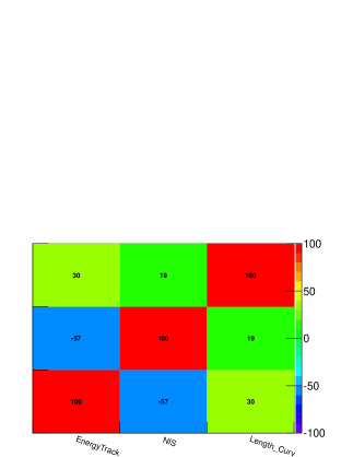
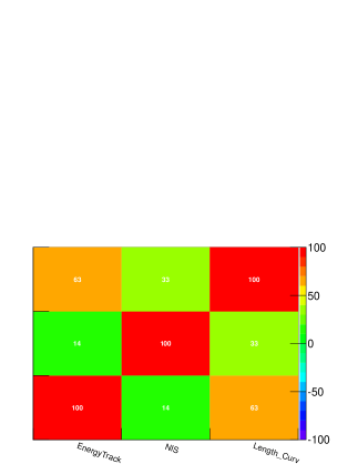
Figure 3 (third row, second column) presents the distributions in the (NIS, $L_{c}$) plane. This highlights the complementarity between these two observables. While the electron distribution extends to large curve length values with a constant NIS value, fluorine recoils are characterized by short curve length, below 3 cm, and NIS value ranging between $10^{-3}$ and 1. To check for correlations, we present on figure 4 the correlation matrix between the different observables, for fluorine recoils (left) and electron recoils (right). First, we notice that the ionization energy and the NIS observable are not correlated for nuclear recoils (14%) and strongly anticorrelated for electrons ($\sim-60\%$). On the contrary, the curve length is slightly correlated ($\sim 30\%$) for electrons and strongly for fluorine recoils ($\sim+60\%$). Eventually, the NIS and curve length are only slightly correlated ($\sim 30\%$ for fluorine recoils and $\sim 20\%$ for electrons). Moreover, their correlation with the energy are of opposite sign and clearly different for electron and fluorine recoils. Hence, the use of these discriminant observables seem to be promising for e/recoil discrimination. From this discriminant study, we can conclude that the event tagging will be very efficient above $\sim$ 20 keV, even with a straightforward cut-based analysis (sec. 2). Below 20 keV, an advanced data analysis is needed and we propose a boosted decision tree method for this purpose (sec. 3).

Figure 4: Correlation matrix of the different observables, for fluorine recoils (left) and electron recoils (right). The various observables are indicated on the plot : $E_{ion}$, NIS and $L_{c}$.

Figure 5: Event distributions when selecting events within the 95% CL recoil acceptance region on various observables. Blue points present the events simulated as nuclear recoil whereas the red crosses present the simulated electrons. Left upper panel : (NIS, ionization energy) plane for a selection on the curve length observable only. Right upper panel : (curve length, ionization energy) for a selection on the NIS observable only. Lower panels : (NIS, ionization energy) plane and (curve length, ionization energy) plane after a selection on both NIS and curve length observables.

2 Sequential analysis

The discriminant observables ($E_{ion}$, $L_{c}$ and NIS) are first used within the framework of a sequential analysis. The goal is to evaluate the signal efficiency ($\mathscr{A}$), i.e. the fraction of nuclear recoils accepted by the analysis, as well as the background rejection power (R). In the following, the rejection power R reads as :

$$R(E_{ion})=\frac{N_{e}}{N_{e}^{selec}}$$ (3)

where $N_{e}$ is the number of electrons in the data sample, of a given energy for instance, and $N_{e}^{selec}$ after applying the electron/recoil discrimination. Note that the rejection power should be defined, for a given confidence level, with an upper value on $N_{e}^{selec}$, following a Poisson statistics. We nevertherless stick to this standard definition for the sake of comparison with rejection powers from others Dark Matter experiments.

2.1 Defining cuts on the observables

To define the cuts on the observables, the 95% CL region on each observable ($L_{c}$ and NIS) have been evaluated as a function of the ionization energy. The sequential analysis consists in rejecting all event outside the nuclear recoil acceptance region, defined as the region within the 95% CL nuclear recoil region minus its intersection with the 95% CL electron region.
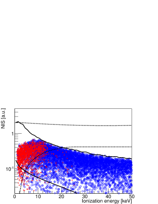
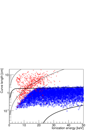
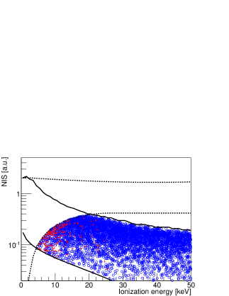
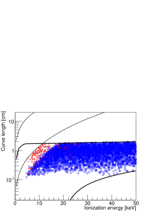
As an illustration, figure 5 presents event distributions when selecting events within the 95% CL recoil acceptance region on various observables. Blue points present the events simulated as nuclear recoil whereas the red crosses present the simulated electrons. The left upper panel presents the event distribution in the (NIS, ionization energy) plane, when selecting events within the 95% CL recoil acceptance region on the curve length observable only. It can first be noticed that a substantial electron contamination remains within the recoil acceptance region. However they lie within the electron acceptance region and a large fraction will be removed by a selection on the NIS variable. Figure 5 (upper right panel) presents the event distribution in the (curve length, ionization energy) plane, when selecting events within the 95% CL recoil acceptance region on the NIS observable only. Most electrons accepted by the NIS selection will be rejected by the curve length cut as they lie outside the recoil acceptance region, while loosing very few nuclear recoils. This highlights the complementarity between these two discriminant observables. It is worth emphasizing that the NIS cut implies a high energy threshold ($\sim$ 4 keV), much larger than in the case of $L_{c}$ cut ($\lesssim 1\ {\rm keV}$). The efficiency at low energy is also expected to be rather small in this case.
As a matter of fact, the e/recoil discrimination must include a selection on both discriminant observables (NIS and $L_{c}$). The recoil acceptance is now defined in a 3D observable space (NIS, $L_{c}$ and $E_{ion}$), with cuts an the projection on each plane as discussed above. Figure 5 (lower panels) presents the result of this selection in the (NIS, ionization energy) plane and in the ($L_{c}$, ionization energy) one. It can be seen that the combined selection allows to reduce the electron contamination within the recoil acceptance region. However, the 4 keV threshold associated to the NIS selection remains, as only hard-cuts are used in this analysis.

Figure 6: Efficiency (left panel) and the rejection power (right panel) as a function of the ionization energy, in the case of a cut on the curve length only (blue), on the NIS observable only (red) and for a combined cut on the two observables (black).

2.2 Rejection and efficiencies

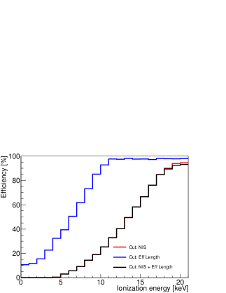
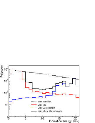
Figure 6 presents the efficiency (left panel) and the rejection power (right panel) as a function of the ionization energy. In the case of a cut on the curve length only (fig. 6 blue curves), the efficiency raises from 10% to 95% when the ionization energy increases from 0 to 10 keV. The rejection power is higher than 100 above 15 keV. For a cut on the NIS observable only (fig. 6 red curves), it is worth emphasizing that a 4 keV threshold is observed, above which the efficiency increases with the ionization energy to reach 95% at 20 keV. Due to this energy threshold, the rejection values below 4 keV are not relevant. For a combined cut on the two observables (fig. 6 black curves), the efficiency is very close to the one of the NIS cut, as it is the most stringent cut at low energy. In particular, the 4 keV threshold stands as a major drawback of this analysis strategy. Between 4 and 14 keV, the rejection power is dominated by the effect of the NIS cut, in the vicinity of 100. Above 14 keV, the effect of the $L_{c}$ cut becomes dominant and the rejection power of the combined cut is increasing, reaching 1000 at 20 keV. Above this energy, the e/recoil is expected to increase with energy as the two distributions start to be well separated (see fig. 2).

3 Event tagging by Boosted Decision Tree analysis

Above 20 keV (ionization), a sequential analysis is probably sufficient to achieve high rejection power against electron together with a high recoil efficiency. Indeed, the two distributions are well separated in the observable space (NIS, $L_{c}$ and $E_{ion}$). However, at low energy, the efficiency obtained with such an analysis starts decreasing with decreasing energy. At 15 keV (ionization), it is of the order of 50% and a 4 keV threshold is observed. For rare event search, such as WIMP dark matter, we argue that this should be improved. In particular, other effects are expected to raise the energy threshold (e.g. quenching factor, 3D reconstruction, …) and the e/recoil discrimination should be optimized to limit its effect at low energy.
For this purpose a multivariate analysis is proposed in order to improve electron/recoil discrimination at low energy. It is a Boosted Decision Tree (BDT) analysis, based on the same discriminant observables.

3.1 Introduction to BDT analysis

Boosted Decision Tree (BDT) analysis belongs to machine learning techniques and is widely used to treat data in high energy physics (e.g. [47, 48, 49]). It is an extension of the commonly used cut-based selection strategy into a multivariate technique. Decision Tree analysis can be seen as a data classifier and is often used for signal/background discrimination. Indeed, as most events do not have all characteristics of either signal or background, the principle of Decision Tree is to keep events that fail a given criterion and check for other observable discriminants. Trees can then be boosted to combine weak classifiers into a new one with smaller error rate [50].
The result of a BDT analysis is given by a forest of $N_{trees}$ decision trees ($T_{k}$) combined in a unique variable $X_{BDT}$, containing all the information. It reads as :

$$X_{BDT}=\sum_{k=1}^{N_{trees}}\alpha_{k}T_{k}(\tilde{O}^{l})$$ (4)

where $\tilde{O}^{l}$ are the discriminant observables and $\alpha_{k}$ the weight of each tree $T_{k}$.
Boosting is then applied to increase the weight of misclassified events in order to reduce the misclassification rate of the next tree. Note that the misclassification rate can be reduced to zero, but at the price of overtraining. This appears when trees contain to many leafs, with a low number of events. In this case, the algorithm is sensitive to statiscal fluctuations of the training sample. A Kolmogorov statistical test on cumulative distributions associated to the test sample and to the training sample is used to check for overtraining.
In a previous paper [36], we have proposed a new method to optimize the sense recognition efficiency for 3D track reconstruction of directional data. We extend this idea to improve the recoil efficiency of e/recoil discrimination at low energy. In the following, we acknowledge the use of the TMVA software [51].

3.2 BDT analysis for e/recoil discrimination

To apply BDT analysis to e/recoil discrimination, we use the same observables as for the sequential analysis, namely NIS, $L_{c}$ and $E_{ion}$. Two data populations are used (electrons and nuclear recoils). Trees have been trained with 10⁵ events (nuclear recoils and electrons). To avoid overtraining while maximizing the performance of the BDT analysis, a minimum number of 100 events per leaf is required as well as a maximum number of tree levels of 50. We found this configuration to be optimal as it stands at the limit of overtraining. Indeed, following the Kolmogorov test statistic, we found a maximal distance between the train and test sample cumulative distributions of $5.87\times 10^{-3}$ corresponding to a p-value of $7.7\times 10^{-2}$. This result suggests a 2$\sigma$ agreement between the two distributions validating our statement that the Boosted Decision Tree algorithm considered in the following is not overtrained.

Figure 7: Left : $X_{BDT}$ distributions for electrons (red) and nuclear recoils (blue). Right : electron efficiency as a function of the nuclear recoil efficiency in the case of this analysis applied on the simulated electron and nuclear recoil distributions.

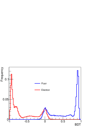
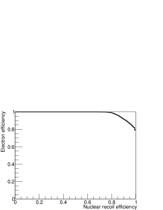
Figure 7 (left) presents the $X_{BDT}$ distributions for electrons (red) and nuclear recoils (blue). In the following, we aim at selecting nuclear recoils while rejecting electrons. Hence events need to be tagged either as electrons or nuclear recoils. Such event tagging is achieved by applying a cut on the value of $X_{BDT}$. This implies, for each cut value, a given efficiency and rejection that can then be easily estimated. Figure 7 (right) presents the electron efficiency as a function of the nuclear recoil efficiency in the case of this analysis is applied on the simulated electron and nuclear recoil distributions. We can conclude from this figure, that an electron efficiency above 90% implies a nuclear recoil efficiency below 90%.
There is two ways to use a BDT analysis : either events tagged as electrons are rejected (sec. 3.4) or all events are kept and weighted according to their electron probability (sec. 3.3).

Figure 8: Event distribution after event tagging : ($L_{c}$ vs $E_{ion}$) left (NIS vs $E_{ion}$) right. The color code indicates the value of $w_{i}$, i.e. the probability to be nuclear recoil.

3.3 Probability weighting method

For a given event, the value of $X_{BDT}$ is related to its probability to be a nuclear recoil $w_{i}$, via the Bayes’ theorem. It is defined from the conditional distributions $f(X_{BDT}|{\rm electron})\equiv f_{e}(X_{BDT})$ and $f(X_{BDT}|{\rm fluor})\equiv f_{f}(X_{BDT})$ (cf. figure 7) as:

$$w_{i}=\frac{f_{f}(X^{i}_{BDT})}{f_{e}(X^{i}_{BDT})+f_{f}(X^{i}_{BDT})}.$$ (5)

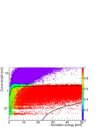
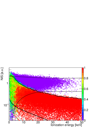
Figure 8 presents all events in the (NIS, $E_{ion}$) plane (right) and in the ($L_{c}$, $E_{ion}$) one (left) where the color code is related to their probability to be a nuclear recoil $w_{i}$. Acceptance regions from the sequential analysis are recalled to ease comparison. Most events in the 95% acceptance nuclear recoil region are tagged as such. Above 20 keV, the discrimination is almost perfect and events are tagged either as electrons or nuclear recoils with a null misidentification. Interestingly, below 20 keV a fraction of events are identified as nuclear recoils whereas they lie well outside the nuclear recoil acceptance region. Hence, they would have been missed by a sequential analysis. Below 10 keV a large numbers of events are associated with a probability $0<w_{i}<1$ associated with an ambiguous identification. Whereas a hard cut on the value of BDT would remove them and hence decrease the efficiency, it is possible to decrease their effect on Dark Matter search, by taking into account their probability to be a nuclear recoil or an electronic recoil.

Figure 9: Distribution in the (BDT, $E_{ion}$) plane for electronic events (red crosses) and fluorine recoils (blue circles).

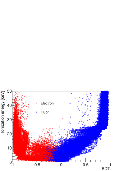
To perform such analysis without using hard cuts on the $X_{BDT}$ value, we defined the following likelihood function aiming at fitting all the recorded events in the $\{E_{r}(\equiv E_{ion}),\Omega_{r},L_{c},NIS\}$ parameter space. The observables $E_{ion}$, $L_{c}$ and $NIS$ can be transformed into a unique variable, $X_{BDT}$, following the distributions shown on figure 7 (left). However, we found that there is a strong correlation between $X_{BDT}$ and $E_{ion}$ (see fig. 9) implying that the likelihood function from [5, 6, 7] must be modified as follows :

$$\mathscr{L}(\vec{\theta})= \frac{e^{-\mu_{\rm tot}}}{N!}$$

$$\times\prod_{i=1}^{N}\left[\left(\mu_{s}S(\vec{R}_{i})+\mu_{n}N(\vec{R}_{i})\right)\times f_{f}(X^{i}_{BDT}|E_{i})+\mu_{e}E(\vec{R}_{i})\times f_{e}(X^{i}_{BDT}|E_{i})\right]$$

with $\mu_{\rm tot}$ defined as :

$$\mu_{\rm tot}=\mu_{s}+\mu_{n}+\mu_{e}$$ (7)

where $\mu_{s}$, $\mu_{n}$ et $\mu_{e}$ correspond to the expected mean number of WIMP, neutron and electron events respectively, which are part of the free parameters ($\vec{\theta}$) of the likelihood function and $N$ is the total number of events measured.
The function $S(\vec{R}_{n})$, $N(\vec{R}_{n})$ and $E(\vec{R}_{n})$ correspond to the $d^{2}N/dE_{r}d\Omega_{r}$ distributions associated with WIMP, neutron and electron events respectively. $\vec{R}_{i}$ refers to the characteritics of the $i$-th event (recoil energy $E_{r}$ and direction $\Omega_{r}$). The functions $f_{f}(X_{BDT}|E)$ and $f_{e}(X_{BDT}|E)$ correspond to the normalized conditional probability distributions of $X_{BDT}$ depending on the energy. These distributions can easily be estimated from the figure 9 which shows that there is a strong correlation between $X_{BDT}$ and $E_{ion}$. Indeed, greater is the ionization energy, better is the discrimination between the two popullations leading to distributions more peaked around -1 for the electrons and +1 for the fluorine recoils. The non-correlation between $X_{BDT}$ and $\Omega_{r}$ is simply explained by the fact that $L_{c}$ and $NIS$ are weakly correlated with the orientation of the track in the detector frame due to primary electron diffusion and detector limitations (pixel size and time sampling of the anode). Moreover, from the detector frame to the galactic frame, there is several rotations smearing out any residual correlations between the direction of the recoil in galactic coordinates and $X_{BDT}$.

Hence, this analysis strategy allows to account for all events which has the benefit of maximizing the efficiency and then the Dark Matter reach of a given directional detector (see sec. 4). This way, if no events is observed, we keep a 100% efficiency. Estimation of the effect of such analysis on the discovery and exclusion potential is beyond the scope of this paper.

3.4 Cut-based BDT method

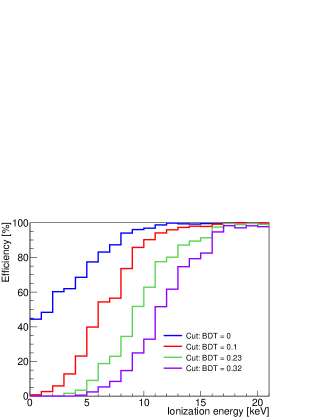
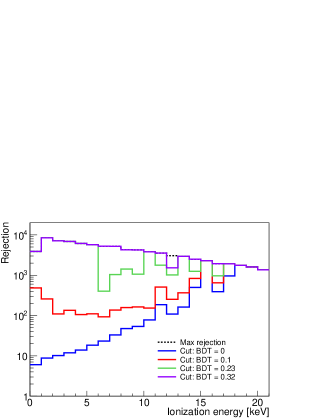
Another way to use BDT analysis is to select only events above a given value of $X_{BDT}$. Hereafter, this event tagging method is referred to as cut-based BDT analysis. Efficiencies and rejections are then estimated as explained above (see fig. 7). All events associated with $X_{BDT}$ value greater than a threshold value, X_cut, are tagged as nuclear recoils whereas all events with BDT value below this value are rejected.

Figure 10 presents the efficiency (left) and the rejection (right) as a function of the ionization energy, for several values of X_cut. For a value X_cut = 0, we notice that there is no threshold effect induced by this discrimination strategy. At 0 keV, the efficiency is $\sim 50\%$ and increases with ionization energy to reach 90% around 10 keV. For this selection, the rejection against electrons starts at 10 at 0 keV and reaches 1000 around 20 keV. For a value X_cut = 0.1, the efficiency reaches 50% at 5 keV (ionization) and implies a rejection against electrons always above 100. As expected, increasing the value of X_cut results in a loss of efficiency and an increase of rejection. We caution that the higher value of rejection (X_cut=0.32) are limited by the number of events generated in this simulation. They must hence be taken as a minimum value.
Interestingly, the BDT analysis alleviates the threshold effect observed in fig. 6 and allows for high rejection power together with high efficiencies below 20 keV (ionization). It is worth emphasizing this upper value chosen for this analysis. First, and as stated above, the discrimination above 20 keV (ionization) efficient even with a sequential analysis. The expected rejection values are very high ($>10^{3-4}$), noticing that these values correspond to a flat electron spectrum, between 0 and 50 keV. Moreover, 20 keV (ionization) corresponds to about 50 keV (recoil) when taking into account the Fluorine Ionization Quenching Factor.
We conclude that cut-based BDT analysis provides a powerful way to discriminate electron from nuclear recoils at low energy. This event tagging strategy is of general interest for Dark Matter search and could be adapted for various e/recoil discrimination strategies. In fine, the level of rejection needed can be tuned by choosing the value of X_cut. It is then a matter of choice to set a priority either on the efficiency or on the rejection. This issue is closely related to radiopurity of the chosen material and Dark matter search strategy. Indeed, as outlined in [6, 7], directional detection could accommodate to a sizeable background contamination, thanks to the evaluation of the double-differential spectrum $\mathrm{d}^{2}R/\mathrm{d}E_{R}\mathrm{d}\Omega_{R}$. Moreover, as shown in [36], the reconstruction of the localization of the vertex of event in the detector volume is a key issue in order to discriminate surface events, mostly coming from the radioactivity from the surrounding detector material. It allows to define a fiducial cut which will considerably reduce the background event contamination of the data, prior to the e/recoil discrimination.

Figure 10: Efficiency (left) and the rejection (right) as a function of the ionization energy, for several values of X_cut : X_cut = 0 (blue), X_cut = 0.1 (red), X_cut = 0.23 (green) et X_cut = 0.32 (purple).

4 Consequences for Dark Matter search

A cut-based BDT analysis would provide a high rejection against electrons and a good efficiency, depending on the choice of cut on the BDT variable. In this section, we investigate the consequences for Dark Matter search potential in the case of the 30 kg.year MIMAC detector. First, we evaluate the event rate in the ionization energy range, taking into account the selection efficiency from this e/recoil discrimination. In the following we note the latter as $\mathscr{A}(E_{\rm ion})$. It depends both on the ionization energy (fig. 10) and on the value of BDT_cut. The total number of WIMP events, $\mu_{s}$, reads as :

$$\mu_{s}=\int_{E_{\rm ion}^{1}}^{E_{\rm ion}^{2}}\left[\int_{0}^{\infty}\frac{dR}{dE_{\rm ion}}(E_{\rm ion}^{\prime})\times K(E_{\rm ion}^{\prime},E_{\rm ion})\times\epsilon(E_{\rm ion}^{\prime})dE_{\rm ion}^{\prime}\right]\times\mathscr{A}(E_{\rm ion})dE_{\rm ion}$$ (8)

where $\epsilon$ is the detection efficiency, i.e. events having $N_{c}>1$ and fully enclosed within the detector, $Q(E_{r})$ is the average value of the ionization quenching. $K(E_{r},E_{\rm ion})$ is the energy resolution of the detector, taking into account fluctuations in the energy loss channel, the number of electron/ion pairs and the amplification.
The selection efficiency, $\mathscr{A}(E_{\rm ion})$, is evaluated in the following within the framework of a sequential analysis (sec. 2), as well as a boosted decision tree method (sec. 3). $\mu_{s}$ is Monte Carlo evaluated with 10⁵ WIMP events with an energy range between 0 and 160 keV.

Figure 11: Ionization energy spectra for WIMP mass $m_{\chi}=100$ GeV.c^-2, for a rejection power : $R=10$ (X_cut = 0) in blue, $R=100$ (X_cut = 0.1) in red, $R=1000$ (X_cut = 0.23) in green et $R=10000$ (X_cut = 0.32) in purple. The black distribution presents the case where no selection is applied on the BDT variable.

Figure 12: Sensitivity of a 30 kg.year $CF_{4}$ directional detector (MIMAC). The result is presented as a limit in ($\sigma_{p},m_{\chi}$), where $\sigma_{p}$ is the spin-dependent cross section on nucleon and $m_{\chi}$ the WIMP mass. The dashed red curve represents the sensitivity without cuts. The sensitivity for the loose cut case is presented as a dashed black curve. Rejections obtained with a BDT analysis are presented : $R=10$ in blue, $R=100$ in red, $R=1000$ in green and $R=10^{4}$ in purple. The sensitivity for sequential analysis, with a rejection R=528, is presented as a dotted black curve.

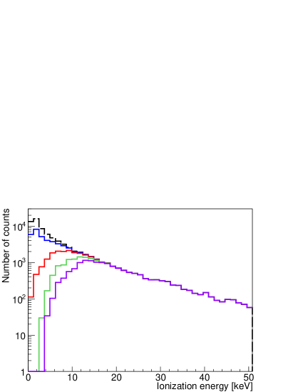
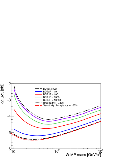
Figure 12 presents the ionization energy spectra for WIMP mass $m_{\chi}=100$ GeV.c^-2, for a rejection power : $R=10$ (X_cut = 0) in blue, $R=100$ (X_cut = 0.1) in red, $R=1000$ (X_cut = 0.23) in green et $R=10^{4}$ (X_cut = 0.32) in purple. The black distribution presents the case where no selection is applied on the BDT variable ($\mathscr{A}(E_{\rm ion})=1$). It shows the impact of : the loose selection (events having $N_{c}>1$ and fully enclosed within the detector), the ionisation quenching factor (conversion from recoil energy to ionization energy) and the energy resolution. Note that would be the case for the weighting probability method.
As expected, an increase of the rejection power, via a tighter cut on X_cut, implies a loss of low energy events. For a rejection $R=10^{4}$ it corresponds to a 4 keV threshold. It is worth emphasizing that the rejection values cited hereabove correspond to a flat electron spectrum, between 0 and 50 keV. Hence, these values must be taken as reference values and they must be treated with caution when compared to experimental values, obtained from a $\gamma$-ray source [52].

Figure 12 presents the sensitivity of a 30 kg.year $CF_{4}$ directional detector (MIMAC) [7]. The result is presented as a limit in ($\sigma_{p},m_{\chi}$), where $\sigma_{p}$ is the spin-dependent cross section on proton and $m_{\chi}$ the WIMP mass. The sensitivity is defined as the Poisonnian limit with 0 event measured. The recoil energy range chosen for this sudy is 5-50 keV, which correspond to an ionization energy range of 0.5-17.5 keV, when taking into account the ionization quenching factor as obtained from SRIM simulations [46]. The dashed red curve represents the sensitivity without cuts. It stands as the ultimate reach for such an exposure. The sensitivity for the loose cut case is presented as a dashed black curve. Interestingly, it is also the sensitivity expected for the weighting probability method in the 0 event case. The effect of such a selection on the sensitivity of the MIMAC detector is shown to be weak. Rejections obtained with a BDT analysis are presented : $R=10$ in blue, $R=100$ in red, $R=1000$ in green and $R=10^{4}$ in purple. The sensitivity for sequential analysis, with a rejection R=528, is presented as a dotted black curve. It can be noticed that increasing the rejection results in a loss of sensitivity to low mass WIMPs. Reaching $R=10^{4}$, the loss of sensitivity is of the order of one order of magnitude at high WIMP mass. As stated above, the choice of the rejection power value, through the choice of the value of X_cut, is related to the acceptable level of background contamination. Eventually, we highlight the fact that a Boosted Decision Tree e/recoil discrimination strategy would have a rejection $\sim 20$ times higher than a sequential analysis, for the same Dark Matter exclusion reach.

5 Conclusion

Even though it could accommodate to a sizeable background contamination, electron/recoil discrimination remains a key and challenging issue as for direction-insensitive detectors. In the case of low pressure TPCs dedicated to directional search, the event background rate can be reduced through fiducialization, thanks to the good spatial resolution along the three axes [36]. Nonetheless, electron/recoil discrimination remains a key and challenging issue. While a high rejection power is expected at high energy (above 20 keV), a dedicated data analysis is needed at low energy. After identifying discriminant observables, a multivariate analysis, namely a Boosted Decision Tree, is proposed, enabling an efficient event tagging for Dark Matter search. We show that it allows us to optimize rejection while keeping a rather high efficiency which is compulsory for rare event search.With respect to a sequential analysis, the rejection is about $\sim 20$ times higher with a multivariate analysis, for the same Dark Matter exclusion limit. This event tagging strategy is of general interest for Dark Matter search and could be adapted for various e/recoil discrimination strategies.

References

- [1] D. N. Spergel, Phys. Rev. D 37 (1988) 1353
- [2] D. Albornoz Vásquez, G. Bélanger, J. Billard and F. Mayet, Phys. Rev. D 85 (2012) 055023
- [3] D. S. M. Alves, S. E. Hedri and J. G. Wacker, arXiv:1204.5487 [astro-ph.GA].
- [4] J. Billard, F. Mayet, J. F. Macias-Perez and D. Santos, Phys. Lett. B 691 (2010) 156-162
- [5] J. Billard, F. Mayet and D. Santos, Phys. Rev. D 83 (2011) 075002
- [6] J. Billard, F. Mayet and D. Santos, Phys. Rev. D 85 (2012) 035006
- [7] J. Billard, F. Mayet and D. Santos, Phys. Rev. D 82 (2010) 055011
- [8] N. Bozorgnia, G. B. Gelmini and P. Gondolo, arXiv:1111.6361 [astro-ph.CO].
- [9] C. -T. Chiang, M. Kamionkowski and G. Z. Krnjaic, arXiv:1202.1807 [astro-ph.CO].
- [10] C. J. Copi and L. M. Krauss,, Phys. Rev. D 63 (2001) 043507
- [11] C. J. Copi, L. M. Krauss, D. Simmons-Duffin and S. R. Stroiney, Phys. Rev. D 75 (2007) 023514,
- [12] C. J. Copi and L. M. Krauss, Phys. Lett. B 461 (1999) 43
- [13] R. J. Creswick, S. Nussinov and F. T. Avignone, Astropart. Phys. 35 (2011) 62
- [14] M. Kuhlen, M. Lisanti and D. N. Spergel, arXiv:1202.0007 [astro-ph.GA].
- [15] S. K. Lee and A. H. G. Peter, JCAP 1204 (2012) 029
- [16] M. Lisanti and J. G. Wacker, Phys. Rev. D 81 (2010) 096005
- [17] A. M. Green and B. Morgan, Phys. Rev. D 77 (2008) 027303
- [18] A. M. Green and B. Morgan, Astroparticle Physics 27 (2007) 142
- [19] A. M. Green and B. Morgan, Phys. Rev. D 81 (2010) 061301
- [20] B. Morgan and A. M. Green, Phys. Rev. D 72 (2005) 123501
- [21] B. Morgan, A. M. Green and N. J. C. Spooner, Phys. Rev. D 71 (2005) 103507
- [22] S. Ahlen et al., Int. J. Mod. Phys. A 25 (2010) 1
- [23] S. Ahlen et al., Phys. Lett. B695 (2011) 124-129
- [24] E. Daw et al., Astropart.Phys. 35 (2012) 397-401
- [25] S. E. Vahsen et al., EAS Publications Series 53 (2012) 43-50
- [26] D. Santos et al., EAS Publications Series 53 (2012) 25-31
- [27] K. Miuchi et al., Phys. Lett. B 686 (2010) 11
- [28] B. Censier, EAS Publications Series 53 (2012) 59-66
- [29] Z. Ahmed et al., Phys. Rev. Lett. 106 (2011) 131302
- [30] E. Armengaud et al., Phys. Lett. B 702 (2011) 329
- [31] E. Aprile et al., Astropart. Phys. 35 (2012) 573
- [32] E. Aprile et al., Phys. Rev. D. 72 (2005) 072006
- [33] G. Angloher et al., arXiv:1109.0702 [astro-ph.CO].
- [34] E. Moulin, PhD Thesis, Université Joseph Fourier, Grenoble (France), Sept. 2005
- [35] D. Santos, E. Moulin, F. Mayet and J. Macias-Perez, J. Phys. Conf. Ser. 39 (2006) 154
- [36] J. Billard, F. Mayet and D. Santos, JCAP 04 (2012) 006
- [37] Y. Giomataris et al., Nucl. Instrum. Meth. A 560 (2006) 405
- [38] F. J. Iguaz et al., JINST 6 (2011) P07002
- [39] J. P. Richer et al., Nucl. Instrum. Meth. A 620 (2010) 470
- [40] O. Bourrion et al., Nucl. Instrum. Meth. A 662 (2010) 207
- [41] O. Bourrion et al., EAS Publications Series 53 (2012) 129-136
- [42] O. Guillaudin et al., EAS Publications Series 53 (2012) 119-127
- [43] J. Billard, PhD Thesis, Université Joseph Fourier, Grenoble (France), June 2012
- [44] S. F. Biagi, Nucl. Instrum. and Meth. A 421 (1999) 234-240
- [45] S. Agostinelli, Nucl. Instrum. Meth. A 506 (2003) 250-303
- [46] J. F. Ziegler, J. P. Biersack and U. Littmark U., Pergamon Press New York, (1985), www.srim.org.
- [47] B. P. Roe et al., Nucl. Instrum. Meth. A 543 (2005) 577-584
- [48] V. M. Abazov et al. Phys. Rev. D 78 (2008) 012005
- [49] J. Conrad and F. Tegenfeldt, JHEP 0607 (2006) 040
- [50] Y. Coadou, EPJ Web of Conferences 4 (2010) 02003, Proceedings of SOS’08, IN2P3 School of Statistics, A. Lucotte & F. Melot (Eds.)
- [51] A. Hoecker et al., PoS ACAT 040 (2007)
- [52] J. P. Lopez et al., arXiv:1109.3501 [astro-ph.IM].