Observational constraints on unified dark matter including Hubble parameter data

Abstract

We constrain a unified dark matter (UDM) model from the latest observational data. This model assumes that the dark sector is degenerate. Dark energy and dark matter are the same component. It can be described by an affine equation of state $P_{X}=p_{0}+\alpha\rho_{X}$. Our data set contains the newly revised $H(z)$ data, type Ia supernovae (SNe Ia) from Union2 set, baryonic acoustic oscillation (BAO) observation from the spectroscopic Sloan Digital Sky Survey (SDSS) data release 7 (DR7) galaxy sample, as well as the cosmic microwave background (CMB) observation from the 7-year Wilkinson Microwave Anisotropy Probe (WMAP7) results. By using the Markov Chain Monte Carlo (MCMC) method, we obtain the results in a flat universe: $\Omega_{\Lambda}$=$0.719_{-0.0305}^{+0.0264}(1\sigma)_{-0.0458}^{+0.0380}(2\sigma)$, $\alpha$=$1.72_{-4.79}^{+3.92}(1\sigma)_{-7.30}^{+5.47}(2\sigma)(\times 10^{-3})$, $\Omega_{b}h^{2}$=$0.0226_{-0.0011}^{+0.0011}(1\sigma)_{-0.0015}^{+0.0016}(2\sigma)$. Moreover, when considering a non-flat universe, $\Omega_{\Lambda}$=$0.722_{-0.0447}^{+0.0362}(1\sigma)_{-0.0634}^{+0.0479}(2\sigma)$, $\alpha$=$0.242_{-0.775}^{+0.787}(1\sigma)_{-1.03}^{+1.10}(2\sigma)(\times 10^{-2})$, $\Omega_{b}h^{2}$=$0.0227_{-0.0014}^{+0.0015}(1\sigma)_{-0.0018}^{+0.0021}(2\sigma)$, $\Omega_{k}$=$-0.194_{-1.85}^{+2.02}(1\sigma)_{-2.57}^{+2.75}(2\sigma)(\times 10^{-2})$. These give a more stringent results than before. We also give the results from other combinations of these data for comparison. The observational Hubble parameter data can give a more stringent constraint than SNe Ia. From the constraint results, we can see the parameters $\alpha$ and $\Omega_{k}$ are very close to zero, which means a flat universe is strongly supported and the speed of sound of the dark sector seems to be zero.

1 INTRODUCTION

Cosmic acceleration is one of the most striking discoveries in modern cosmology acceleration . Many works have been done to explain this unexpected phenomenon. There are different mechanisms for the universe acceleration. The most popular idea is assuming a new component with negative pressure known as dark energy. Other mechanisms contain various modifications of gravitation theory MGR and violation of cosmological principle LTB . There are all kinds of dark energy models including quintessence quintessence , holographic dark energy holographic , quintom quintom , phantom phantom , generalized Chaplygin gas model GCG and so on. Among these, the simplest and most successful model is $\Lambda$CDM model LCDM while it has to face some theoretical problems. For example, the ”coincidence” problem and the ”fine-tuning” problem pr . From this standard model, the flat universe consists of $\sim 4\%$ baryons, $\sim 23\%$ dark matter, $\sim 73\%$ dark energy standard . However, we still know little about dark matter and dark energy unknown . All we can feel about them are their gravitational effects. Observationally, they are degenerate. Based on these, a unified dark matter model was proposed which assumes that dark matter and dark energy are from a same dark component UDM . Since the equation of state of the unified dark component is unknown, we assume that it has a constant speed of sound $c_{s}^{2}=\alpha$ which is equivalent to the affine form constraint . In order to break the degeneracies, different kinds of observational data are used to constrain cosmological model, among which SNe Ia, CMB, and BAO are usually used to constrain cosmological parameters observation . Recently, other observations are included. For example, the gamma-ray burst GRB , cluster gas mass fraction fgas , lensing lensing and so on. But these processes need to integrate the Hubble parameter to obtain the distance scale. The more information about $H(z)$ can’t be embodied. Therefore, it is meaningful to study the $H(z)$ data directly. The expression of the Hubble parameter can be written in this form

$$H(z)=-\frac{1}{1+z}\frac{dz}{dt}\,,$$ (1)

which depends on the differential age as a function of redshift. Based on Jimenez et al. Jimenez , Simon et al. Simon used the age of evolving galaxies and got nine $H(z)$ data. Many works based on these nine data was done nine . Recently, Stern et al. Stern revised these data at 11 redshifts from the differential ages of red-envelope galaxies. Moreover, Gaztañaga et al. three took the BAO scale as a standard ruler in the radial direction, obtained three more additional data.

In this paper, we use the Markov chain Monte Carlo (MCMC) method to give constraints on the unified dark matter model from the latest data including the observational Hubble parameter data. In section 2, we give a brief introduction of the UDM model. In section 3, we introduce the observational data set we use. The full parameter space using different combinations of data is exhibited in section 4. Finally, we give a conclusion in section 5.

2 UNIFIED DARK MATTER WITH CONSTANT SPEED OF SOUND

In this section, we give a brief introduction to unified dark matter model. For details of this model, please refer to UDM .

Considering the universe is described by the Friedmann-Robertson-Walker metric and assuming a single UDM besides baryons and radiation, the Friedmann equation is expressed as

$$H(a)=H_{0}E(a),$$ (2)

where $H_{0}$ represents the Hubble constant today, and

$$E(a)^{2}=\Omega_{r}(a)+\Omega_{b}(a)+\Omega_{X}(a)+\Omega_{k}(a),$$ (3)

where $\Omega_{i}(a)=\rho_{i}(a)/\rho_{c}$, $\rho_{c}$ is the critical density today. The subscripts r, b, k and X represent for radiation, baryons, curvature and UDM component respectively. Each component satisfies the energy-momentum conservation equation

$$\dot{\rho}_{i}=-3H(\rho_{i}+P_{i}).$$ (4)

For the radiation and baryons, the equations of state are $1/3$ and $0$, respectively. The conservation equation gives $\Omega_{b}(a)\propto a^{-3}$ and $\Omega_{r}(a)\propto a^{-4}$.

For the UDM, it is considered as an approximation to an barotropic fluid. Since the equation of state $P_{X}=P_{X}(\rho_{X})$ is unknown, we assume a constant speed of sound

$$dP_{X}/d\rho_{X}\simeq\alpha,$$ (5)

which leads to the 2-parameter affine form

$$P_{X}\simeq p_{0}+\alpha\rho_{X}.$$ (6)

Combined with the conservation equation, we can regard this component as an effective cosmological constant plus a generalized dark matter which has a constant equation of state $\alpha$. The density evolves as

$$\Omega_{X}(a)=\Omega_{\Lambda}+(\tilde{\Omega}_{m})a^{-3(1+\alpha)},$$ (7)

where $\tilde{\Omega}_{m}=\Omega_{Xo}-\Omega_{\Lambda}$ stands for the generalized dark matter, and $\Omega_{\Lambda}$ stands for the effective cosmological constant component, $\dot{\rho}_{\Lambda}=0$.

The Friedmann equation now can be expressed as

$$E(a)^{2}=\Omega_{r}a^{-4}+\Omega_{b}a^{-3}+\Omega_{\Lambda}+(1-\Omega_{b}-\Omega_{r}-\Omega_{\Lambda})a^{-3(1+\alpha)}+\Omega_{k}a^{-2},$$ (8)

where $\Omega_{r}$, $\Omega_{b}$ and $\Omega_{k}$ represent dimensionless radiation, baryon matter and curvature today. $\Omega_{\Lambda}$ and $\alpha$ are the parameters we introduced. We notice that when $\alpha=0$, the UDM model are equivalent to $\Lambda$CDM. In UDM model, we can equivalently think that the generalized dark matter may has a non-zero equation of state. Naturally, because the property of the effective cosmological constant component is the same as the one in $\Lambda$CDM, when the property of generalized dark matter is equivalent to the usual dark matter in $\Lambda$CDM, UDM model totally becomes $\Lambda$CDM.

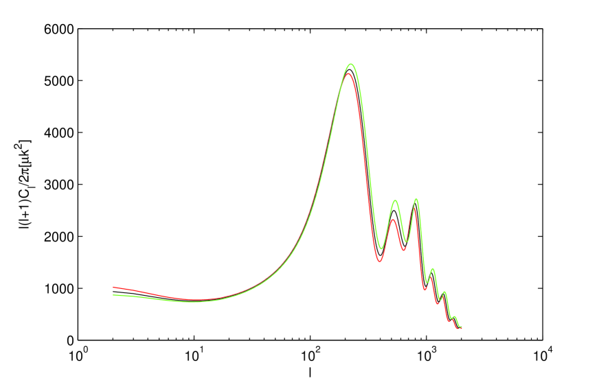
The speed of sound characterizes the perturbations to the dark matter density and pressure which are related to the microphysics. Since we know litter about dark sector in our universe, the equation of state is introduced to describe the property of dark sector. However, it can not give us the information about the microphysics and other properties. The speed of sound can give information about the internal degrees of freedom. For example, quintessence has $c_{s}=1$. If we can confirm the sound speed that is below the speed of light, we can get further degrees beyond a canonical, minimally coupled scalar field. If the sound speed is small, the perturbations can be detected on a proper scale. This perturbations will change the gravitational potential, thus affecting the geodesic of photons. As a result, the cosmic microwave background will be changed through the Integrated Sachs-Wolfe (ISW) effect. In order to show the differences between UDM mdoel and $\Lambda$CDM which corresponds to $\alpha=0$, we give the CMB temperature angular power spectrum in Fig. 7. Our calculations are based on CAMB camb .

3 CURRENT OBSERVATIONAL DATA

Now, we introduce the data set using to constrain the UDM model.

3.1 Observational Hubble parameter data

The observational Hubble parameter as a function of redshift has been used to constrain cosmological parameters hzre . For the observational data, we choose 11 data from Stern . These data were obtained through the measurement of differential ages of red-envelope galaxies known as ”differential age method”. The aging of stars can be regarded as an indicator of the aging of the universe. The spectra of stars can be converted to the information of their ages, as the evolutions of stars are well-known. Since we can not observe stars one by one at cosmological scales, we take the spectra of galaxies which contain relatively uniform star population. The surveys including the Gemini Deep Deep Survey GDDS , VIMOS-VLT Deep Survey and SDSS Stern are related to obtaining data. We consider the red-envelope galaxies which are massive with fairly homogeneous star population. Moreover, the data can be obtained from the BAO scale as a standard ruler in the radial direction known as ”Peak Method” three . Though this method, we have three additional data three : $H(z=0.24)=79.69\pm 2.32,H(z=0.34)=83.8\pm 2.96,$ and $H(z=0.43)=86.45\pm 3.27$, which are independent. Plus the measurement of Hubble constant h0 , we totally have 15 data now. The $\chi^{2}$ value of the $H(z)$ data can be expressed as

$$\chi^{2}_{H}=\sum_{i=1}^{15}\frac{[H(z_{i})-H_{obs}(z_{i})]^{2}}{\sigma_{i}^{2}},$$ (9)

where $\sigma_{i}$ is the $1\sigma$ uncertainty of the observational $H(z)$ data.

3.2 Type Ia supernovae

Since the SNe Ia fist revealed the acceleration of the universe, it has been a well-established method for probing dark energy.

Recently, the Supernova Cosmology Project (SCP) released the Union2 data set including 557 samples Union2 . It covers a redshift region 0-1.4. These data have been widely used to investigate dark energy models use . The distance modules is given by

$$\mu_{theory}(z)=5\log_{10}[d_{L}(z)]+\mu_{0},$$ (10)

where $d_{L}(z)$ is the luminosity distance. It is defined as

$$d_{L}(z)=(1+z)r(z),\quad r(z)=\frac{c}{H_{0}\sqrt{|\Omega_{k}|}}{\rm sinn}\left[\sqrt{|\Omega_{k}|}\int^{z}_{0}\frac{dz^{\prime}}{E(z^{\prime})}\right].$$ (11)

The marginalized nuisance parameter marginalized for $\chi^{2}$ is expressed as

$$\chi^{2}=A-\frac{B^{2}}{C}+\ln\left(\frac{C}{2\pi}\right),$$ (12)

where $A=\sum_{i}^{557}{(\mu^{\rm data}-\mu^{\rm theory})^{2}}/{\sigma^{2}_{i}}$, $B=\sum_{i}^{557}{(\mu^{\rm data}-\mu^{\rm theory})}/{\sigma^{2}_{i}}$, $C=\sum_{i}^{557}{1}/{\sigma^{2}_{i}}$, $\sigma_{i}$ is the 1$\sigma$ uncertainty of the observational data.

Note that the expression

$$\chi^{2}_{\rm SNe}=A-\frac{B^{2}}{C},$$ (13)

which coincides to Eq. (12) up to a constant snc , is used in this paper. The constraint results are the same.

3.3 Cosmic microwave background

For CMB, the shift parameters $R$ and $l_{a}$ are important indicators which are related to the positions of the CMB acoustic peaks. These quantities are affected by the cosmic expansion history from the decoupling epoch to today. The shift parameter $R$ is given by cmbr

$$R=\Omega_{\mathrm{m0}}^{1/2}\Omega_{\mathrm{k}}^{-1/2}sinn\bigg{[}\Omega_{\mathrm{k}}^{1/2}\int_{0}^{z_{\ast}}\frac{dz}{E(z)}\bigg{]},$$ (14)

where $\Omega_{\mathrm{m0}}=\tilde{\Omega}_{m}$ (hereafter), since we have defined the generalized dark matter. The redshift $z_{\ast}$ corresponding to the decoupling epoch of photons is given by cmbz

$$z_{\ast}=1048[1+0.00124(\Omega_{b}h^{2})^{-0.738}(1+g_{1}(\Omega_{\mathrm{m0}}h^{2})^{g_{2}})],$$ (15)

with $g_{1}=0.0783(\Omega_{b}h^{2})^{-0.238}(1+39.5(\Omega_{b}h^{2})^{-0.763})^{-1}$, $g_{2}=0.560(1+21.1(\Omega_{b}h^{2})^{1.81})^{-1}$. Moreover, the acoustic scale is related to the distance ratio. It is give by

$$l_{a}=\pi\frac{\Omega_{\mathrm{k}}^{-1/2}sinn[\Omega_{\mathrm{k}}^{1/2}\int_{0}^{z_{\ast}}\frac{dz}{E(z)}]/H_{0}}{r_{s}(z_{\ast})},$$ (16)

where the comoving sound horizon at photo-decoupling epoch is expressed as

$$r_{s}(z_{\ast})={H_{0}}^{-1}\int_{z_{\ast}}^{\infty}c_{s}(z)/E(z)dz.$$ (17)

From WMAP 7 measurement, the best-fit values of the data set is given by cmb

$$\bar{\textbf{P}}_{\rm{CMB}} = \left(\begin{array}[]{c}{\bar{l}_{a}}\\ {\bar{R}}\\ {\bar{z}_{\ast}}\end{array}\right)=\left(\begin{array}[]{c}302.09\pm 0.76\\ 1.725\pm 0.018\\ 1091.3\pm 0.91\end{array}\right).$$ (24)

where $\Delta\bf{P_{\mathrm{CMB}}}=\bf{P_{\mathrm{CMB}}}-\bf{\bar{P}_{\mathrm{CMB}}}$, and the corresponding inverse covariance matrix is

$${\bf C_{\mathrm{CMB}}}^{-1}=\left(\begin{array}[]{ccc}2.305&29.698&-1.333\\ 29.698&6825.270&-113.180\\ -1.333&-113.180&3.414\end{array}\right).$$ (28)

With these, we can calculate the $\chi^{2}$ by cmb

$$\chi^{2}_{\mathrm{CMB}}=\Delta\textbf{P}_{\mathrm{CMB}}^{\mathrm{T}}{\bf C_{\mathrm{CMB}}}^{-1}\Delta\textbf{P}_{\mathrm{CMB}}.$$ (29)

3.4 Baryon acoustic oscillation

The Baryon Acoustic Oscillations we use measure the distance-redshift relation at two redshifts. One is in the clustering of the combined 2dFGRS and SDSS main galaxy samples at $z=0.2$, the other is in the clustering of the SDSS luminous red galaxies at $z=0.35$. Calculated from these samples, the observed scale of the BAO are analyzed to constrain the form of the distance scale. The distance scale of BAO is defined as DV

$$D_{V}(z)=c\left(\frac{z}{\Omega_{k}H(z)}\mathrm{sinn}^{2}[\sqrt{|\Omega_{k}|}\int_{0}^{z}\frac{dz^{\prime}}{H(z^{\prime})}]\right)^{1/3}.$$ (30)

The peak positions of the BAO depend on the ratio of $D_{v}(z)$ to the sound horizon size at the drag epoch. The redshift $z_{d}$ corresponding to the drag epoch when baryons were released from photos is given by

$$z_{d}=\frac{1291(\Omega_{\mathrm{m0}}h^{2})^{0.251}}{[1+0.659(\Omega_{\mathrm{m0}}h^{2})^{0.828}]}[(1+b_{1}(\Omega_{b}h^{2})^{b_{2}})],$$ (31)

where $b_{1}=0.313(\Omega_{\mathrm{m0}}h^{2})^{-0.419}[1+0.607(\Omega_{\mathrm{m0}}h^{2})^{0.674}]^{-1}$ and $b_{2}=0.238(\Omega_{\mathrm{m0}}h^{2})^{0.223}$ baozd . In this paper, we choose the measurement of the distance radio ($d_{z}$) at $z=0.2$ and $z=0.35$ baodz . This quantity is given by

$$d_{z}=\frac{r_{s}(z_{d})}{D_{V}(z)},$$ (32)

where $r_{s}(z_{d})$ is the comoving sound horizon. From the SDSS data release 7 (DR7) galaxy sample, the best-fit values of the data set ($d_{0.2}$, $d_{0.35}$) baodz

$$\bar{\bf{P}}_{\rm matrix} = \left(\begin{array}[]{c}{\bar{d}_{0.2}}\\ {\bar{d}_{0.35}}\\ \end{array}\right)=\left(\begin{array}[]{c}0.1905\pm 0.0061\\ 0.1097\pm 0.0036\\ \end{array}\right),$$ (37)

where the corresponding inverse covariance matrix is

$${\bf C_{\rm matrix}}^{-1}=\left(\begin{array}[]{ccc}30124&-17227\\ -17227&86977\\ \end{array}\right).$$ (40)

The $\chi^{2}$ value of this BAO observation from SDSS DR7 can be calculated as

$$\chi^{2}_{\rm BAO}=\Delta\textbf{P}_{\rm matrix}^{\mathrm{T}}{\bf C_{\rm matrix}}^{-1}\Delta\textbf{P}_{\rm matrix}.$$ (41)

where $\Delta\bf{P_{\mathrm{matrix}}}=\bf{P_{\mathrm{matrix}}}-\bf{\bar{P}_{\mathrm{matrix}}}$.

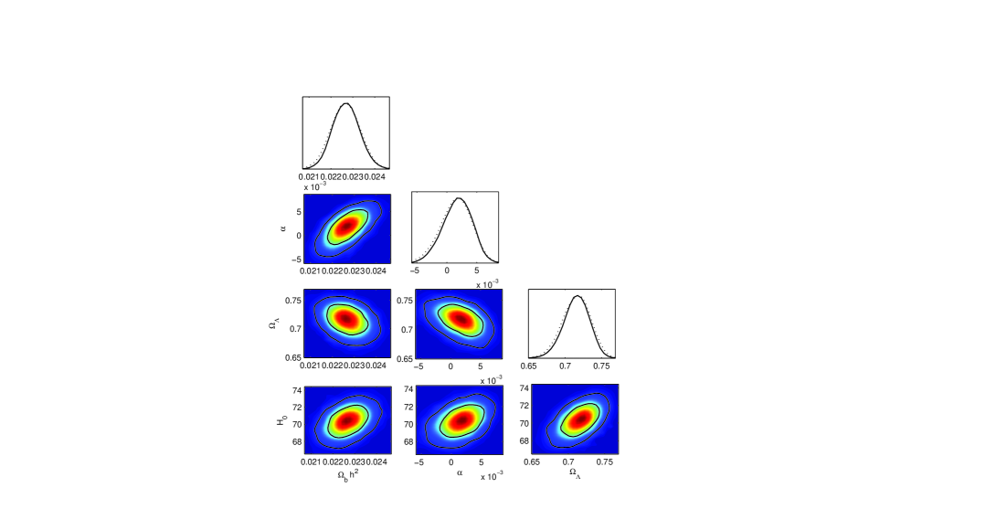
Figure 1: The 2-D regions and 1-D marginalized distribution with the 1-$\sigma$ and 2-$\sigma$ contours of parameters $\Omega_{b}h^{2}$, $\alpha$, $\Omega_{\Lambda}$ in a flat universe, for the data sets $H(z)$+CMB+BAO.

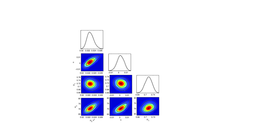
Figure 2: The 2-D regions and 1-D marginalized distribution with the 1-$\sigma$ and 2-$\sigma$ contours of parameters $\Omega_{b}h^{2}$, $\alpha$, $\Omega_{\Lambda}$ in a flat universe, for the data sets SNe+CMB+BAO.

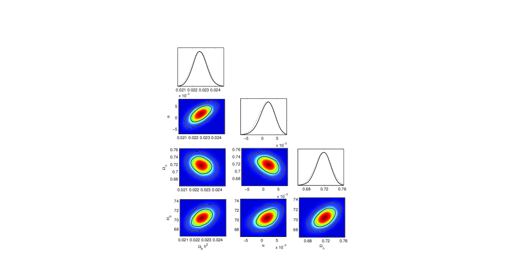
Figure 3: The 2-D regions and 1-D marginalized distribution with the 1-$\sigma$ and 2-$\sigma$ contours of parameters $\Omega_{b}h^{2}$, $\alpha$, $\Omega_{\Lambda}$ in a flat universe, for the data sets $H(z)$+SNe+CMB+BAO.

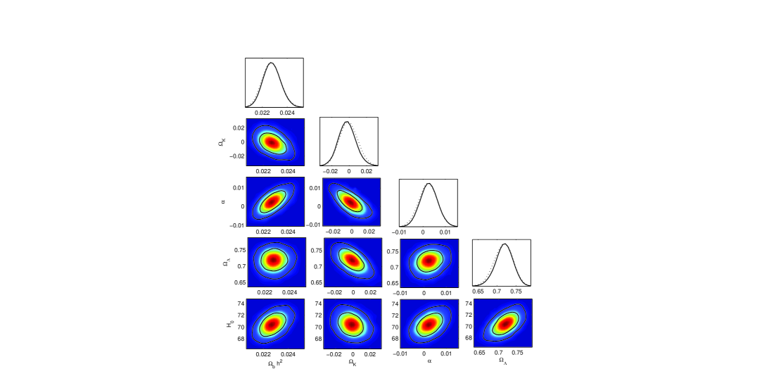
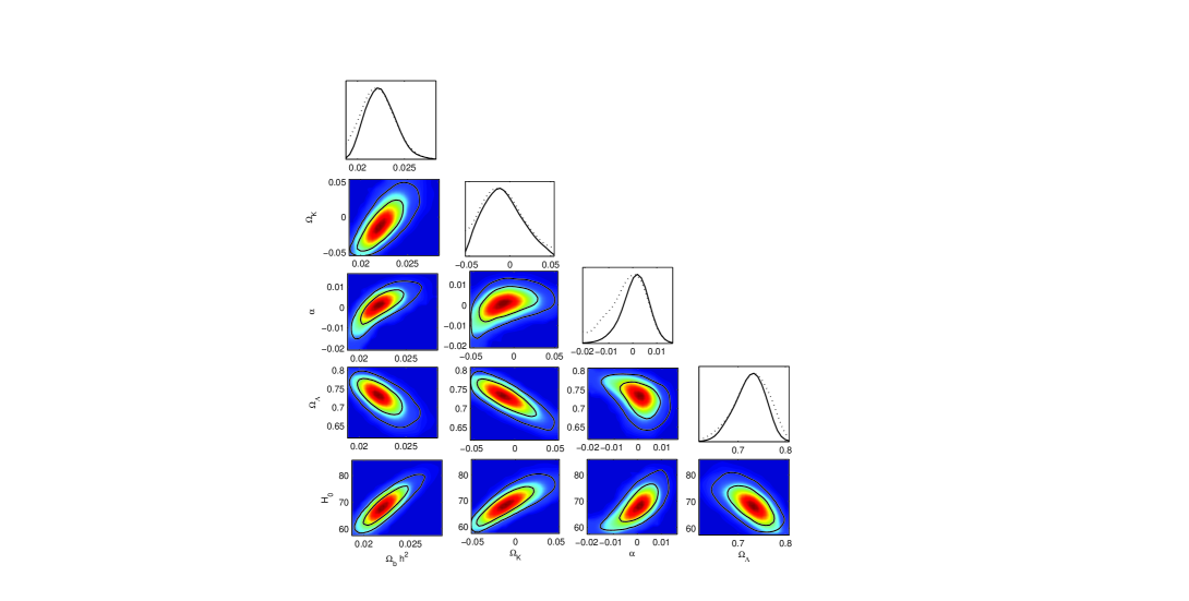
Figure 4: The 2-D regions and 1-D marginalized distribution with the 1-$\sigma$ and 2-$\sigma$ contours of parameters $\Omega_{b}h^{2}$, $\alpha$, $\Omega_{\Lambda}$, $\Omega_{k}$ in a non-flat universe, for the data sets $H(z)$+CMB+BAO.

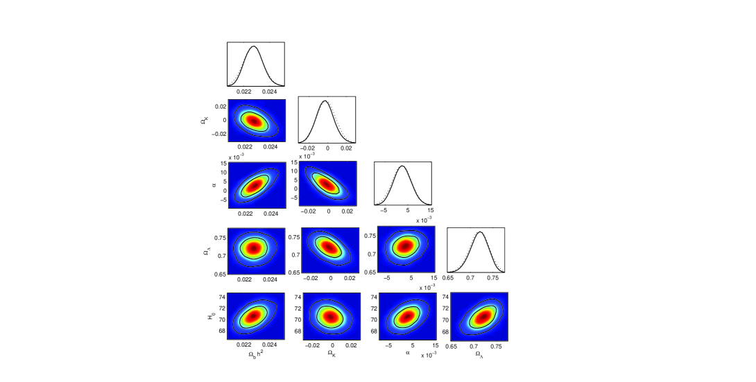
Figure 5: The 2-D regions and 1-D marginalized distribution with the 1-$\sigma$ and 2-$\sigma$ contours of parameters $\Omega_{b}h^{2}$, $\alpha$, $\Omega_{\Lambda}$, $\Omega_{k}$ in a non-flat universe, for the data sets SNe+CMB+BAO.

Figure 6: The 2-D regions and 1-D marginalized distribution with the 1-$\sigma$ and 2-$\sigma$ contours of parameters $\Omega_{b}h^{2}$, $\alpha$, $\Omega_{\Lambda}$, $\Omega_{k}$ in a non-flat universe, for the data sets $H(z)$+SNe+CMB+BAO.

Figure 7: The theoretical CMB temperature angular power spectrum of UDM model. $\alpha=0.01(red),0(black)and-0.01(green)$. $\Omega_{b}h^{2}=0.022,\Omega_{\Lambda}=0.71,H_{0}=70$.

4 CONSTRAINT RESULTS

The statistics we use to constrain parameters is the usual maximum likelihood method of $\chi^{2}$ fitting with the Markov Chain Monte Carlo (MCMC) method. Our code is based on CosmoMCMC mcmc . The corresponding convergence of the chains R-1 is set to be less than 0.003 which can guarantee the accuracy well. We combine $H(z)$, SNe Ia, CMB and BAO data to give a global fitting on determining the parameters of UDM model. The total $\chi^{2}$ is given by

$$\chi^{2}_{tot}=\chi^{2}_{H}+\chi^{2}_{\rm SNe}+\chi^{2}_{\rm CMB}+\chi^{2}_{\rm BAO}.$$ (42)

Fist, we consider a flat universe. In order to embody the $H(z)$ data, we choose three combinations of data sets and show the 1-D probability distribution of each parameter ($\Omega_{b}h^{2}$, $\Omega_{\Lambda}$, $\alpha$) and 2-D plots for parameters between each other. Fitting results from the joint data of $H(z)$+CMB+BAO are given in Fig 1, the best-value for $\alpha$ is $\alpha$=$1.61_{-4.58}^{+3.99}(1\sigma)_{-6.92}^{+5.65}(2\sigma)(\times 10^{-3})$. For comparison, we give the results from SNe+CMB+BAO in Fig 2. The best-fit value is $\alpha$=$1.81_{-8.10}^{+8.15}(1\sigma)_{-11.69}^{+11.99}(2\sigma)(\times 10^{-3})$. We can see the observational Hubble parameter data gives a more stringent constraint than SNe Ia in this model. In Fig 3, the total combinations of them result in $\alpha$=$1.72_{-4.79}^{+3.92}(1\sigma)_{-7.30}^{+5.47}(2\sigma)(\times 10^{-3})$. From the result, the parameter $\alpha$ which stands for the speed of sound of the unified dark sector seems to be vanishing or slightly larger than 0. So $\Lambda$CDM model is strongly supported. We further consider a non-flat universe with curvature. For $H(z)$+CMB+BAO in Fig 4, the results are $\alpha$=$2.21_{-7.60}^{+7.98}(1\sigma)_{-10.91}^{+11.06}(2\sigma)(\times 10^{-3})$, $\Omega_{k}$=$-0.208_{-1.88}^{+2.27}(1\sigma)_{-2.60}^{+3.12}(2\sigma)(\times 10^{-2})$. Using SNe+CMB+BAO in Fig 5, $\alpha$=$0.662_{-22.52}^{+9.80}(1\sigma)_{-37.33}^{+13.68}(2\sigma)(\times 10^{-3})$, $\Omega_{k}$=$-1.41_{-4.83}^{+6.35}(1\sigma)_{-6.46}^{+9.38}(2\sigma)(\times 10^{-2})$. This results are consist with the situation in a flat universe. The $H(z)$ data also gives a much more stringent constraint on $\Omega_{k}$. The total joint data in Fig 6 give $\alpha$=$2.42_{-7.75}^{+7.87}(1\sigma)_{-10.29}^{+11.00}(2\sigma)(\times 10^{-3})$, $\Omega_{k}$=$-0.194_{-1.85}^{+2.02}(1\sigma)_{-2.57}^{+2.75}(2\sigma)(\times 10^{-2})$, which suggest both the speed of sound and the curvature are very little. Our results are much more stringent than previous work constraint . Our results seem to be consistent with $\alpha=0$ using the data sets we select. Does that mean there is no need to introduce a new parameter? We think although the UDM model is contrived, the sound speed of the unified dark matter is related to the microphysics of the dark component while equation of state does not. The sound speed leads to the inhomogeneities of dark matter, thus affecting CMB and matter power spectra. With the development of technique, more information in CMB, matter power spectra and so on may distinguish UDM model from $\Lambda$CDM. Moreover, we assume a constant sound speed, the whole effective value is very small, however, if when we consider the evolving speed of sound, the results may be changed.

	Flat Universe
	$H(z)$+CMB+BAO	SNe+BAO+CMB	$H(z)$+SNe+CMB+BAO
$\Omega_{\Lambda}$	$0.717_{-0.0338}^{+0.0285}(1\sigma)_{-0.0506}^{+0.0404}(2\sigma)$	$0.719_{-0.0353}^{+0.0282}(1\sigma)_{-0.0532}^{+0.0412}(2\sigma)$	$0.719_{-0.0305}^{+0.0264}(1\sigma)_{-0.0458}^{+0.0380}(2\sigma)$
$\alpha$	$1.61_{-4.58}^{+3.99}(1\sigma)_{-6.92}^{+5.65}(2\sigma)(\times 10^{-3})$	$1.81_{-8.10}^{+8.15}(1\sigma)_{-11.69}^{+11.99}(2\sigma)(\times 10^{-3})$	$1.72_{-4.79}^{+3.92}(1\sigma)_{-7.30}^{+5.47}(2\sigma)(\times 10^{-3})$
$\Omega_{b}h^{2}$	$0.0226_{-0.0010}^{+0.0012}(1\sigma)_{-0.0015}^{+0.0017}(2\sigma)$	$0.0227_{-0.0016}^{+0.0022}(1\sigma)_{-0.0022}^{+0.0035}(2\sigma)$	$0.0226_{-0.0011}^{+0.0011}(1\sigma)_{-0.0015}^{+0.0016}(2\sigma)$
$\chi_{\rm min}^{2}$	$11.592$	$532.142$	$542.354$

Table 1: The best-fit values of parameters $\Omega_{b}h^{2}$, $\alpha$, $\Omega_{\Lambda}$ for UDM model in a flat universe with the 1-$\sigma$ and 2-$\sigma$ uncertainties, as well as $\chi_{\rm min}^{2}$, for the data sets $H(z)$+CMB+BAO, SNe+BAO+CMB, and $H(z)$+SNe+BAO+CMB, respectively.

	Non-flat Universe
	$H(z)$+CMB+BAO	SNe+BAO+CMB	$H(z)$+SNe+CMB+BAO
$\Omega_{\Lambda}$	$0.721_{-0.0535}^{+0.0414}(1\sigma)_{-0.0779}^{+0.0549}(2\sigma)$	$0.734_{-0.0815}^{+0.0609}(1\sigma)_{-0.124}^{+0.0799}(2\sigma)$	$0.722_{-0.0447}^{+0.0362}(1\sigma)_{-0.634}^{+0.0479}(2\sigma)$
$\alpha$	$2.21_{-7.60}^{+7.98}(1\sigma)_{-10.91}^{+11.06}(2\sigma)(\times 10^{-3})$	$0.662_{-22.52}^{+9.80}(1\sigma)_{-37.33}^{+13.68}(2\sigma)(\times 10^{-3})$	$2.42_{-7.75}^{+7.87}(1\sigma)_{-10.29}^{+11.00}(2\sigma)(\times 10^{-3})$
$\Omega_{b}h^{2}$	$0.0227_{-0.0013}^{+0.0015}(1\sigma)_{-0.0019}^{+0.0021}(2\sigma)$	$0.0220_{-0.0030}^{+0.0039}(1\sigma)_{-0.0035}^{+0.0056}(2\sigma)$	$0.0227_{-0.0014}^{+0.0015}(1\sigma)_{-0.0018}^{+0.0021}(2\sigma)$
$\Omega_{k}$	$-0.208_{-1.88}^{+2.27}(1\sigma)_{-2.60}^{+3.12}(2\sigma)(\times 10^{-2})$	$-1.41_{-4.83}^{+6.35}(1\sigma)_{-6.46}^{+9.38}(2\sigma)(\times 10^{-2})$	$-0.194_{-1.85}^{+2.02}(1\sigma)_{-2.57}^{+2.75}(2\sigma)(\times 10^{-2})$
$\chi_{\rm min}^{2}$	$11.578$	$531.870$	$542.309$

Table 2: The best-fit values of parameters $\Omega_{b}h^{2}$, $\alpha$, $\Omega_{\Lambda}$, $\Omega_{k}$ for UDM model in a non-flat universe with the 1-$\sigma$ and 2-$\sigma$ uncertainties, as well as $\chi_{\rm min}^{2}$, for the data sets $H(z)$+CMB+BAO, SNe+BAO+CMB, and $H(z)$+SNe+BAO+CMB, respectively.

5 CONCLUSIONS

In this paper, we constrain the unified dark matter with constant speed of sound from the latest data: the newly revised 15 Hubble data, type Ia supernovae (SNe Ia) from Union2 set, baryonic acoustic oscillation (BAO) observation from the spectroscopic Sloan Digital Sky Survey (SDSS) data release 7 (DR7) galaxy sample, as well as the cosmic microwave background (CMB) observation from the 7-year Wilkinson Microwave Anisotropy Probe (WMAP7) results. We consider two case. In a flat universe, the constraint results are $\Omega_{\Lambda}$=$0.719_{-0.0305}^{+0.0264}(1\sigma)_{-0.0458}^{+0.0380}(2\sigma)$, $\alpha$=$1.72_{-4.79}^{+3.92}(1\sigma)_{-7.30}^{+5.47}(2\sigma)(\times 10^{-3})$, $\Omega_{b}h^{2}$=$0.0226_{-0.0011}^{+0.0011}(1\sigma)_{-0.0015}^{+0.0016}(2\sigma)$. In a non-flat universe, the constraint results are $\Omega_{\Lambda}$=$0.722_{-0.0447}^{+0.0362}(1\sigma)_{-0.0634}^{+0.0479}(2\sigma)$, $\alpha$=$0.242_{-0.775}^{+0.787}(1\sigma)_{-1.03}^{+1.10}(2\sigma)(\times 10^{-2})$, $\Omega_{b}h^{2}$=$0.0227_{-0.0014}^{+0.0015}(1\sigma)_{-0.0018}^{+0.0021}(2\sigma)$, $\Omega_{k}$=$-0.194_{-1.85}^{+2.02}(1\sigma)_{-2.57}^{+2.75}(2\sigma)(\times 10^{-2})$. This constraint results are much stringent than previous work constraint , which suggest both the speed of sound of the UDM and the curvature are very little and a flat $\Lambda$CDM model is still a good choice. In order to know the effects of the observational Hubble data, we also consider the combinations $H(z)$+CMB+BAO and SNe+BAO+CMB. From the results, the $H(z)$ data gives a better constraint especially for $\alpha$, $\Omega_{k}$ and $\Omega_{b}h^{2}$ than SNe Ia in this model. We think the $H(z)$ data will paly an important role in cosmology in the future hzfuture .

Acknowledgments We are grateful to Lixin Xu for introducing the MCMC method. We also thank Hao Wang and Jun Wang for helpful discussions. This work was supported by the National Natural Science Foundation of China under the Distinguished Young Scholar Grant 10825313 and Grant 11073005, the Ministry of Science and Technology national basic science Program (Project 973) under Grant No.2012CB821804, the Fundamental Research Funds for the Central Universities and Scientific Research Foundation of Beijing Normal University.

References

• (1) A.G. Riess, et al., Astron. J. 116 (1998) 1009, [arXiv:astro-ph/9805201]; S. Perlmutter, et al., Astrophys. J. 517 (1999) 565, [arXiv:astro-ph/9812133]; A.C. Pope, et al., Astrophys. J. 607 (2004) 655, [arXiv:astro-ph/0401249]; D.N. Spergel, et al., Astrophys. J. Suppl. 148 (2003) 175, [arXiv:astro-ph/0302209].
• (2) G. Lemaitre, Gen. Rel. Grav. 29 (1997) 641; R.C. Tollman, Proc. Nat. Acad. Sci. 20 (1934) 169; H. Bondi, Mon. Not. Roy. Astron. Soc. 107 (1947) 410.
• (3) L. Randall and R. Sundrum, PRL, 83 (1999) 3370; V. Sahni and Y. Shtanov, JCAP, 0311 (2003) 014; S. Capozziello, et al., PRD, 71 (2005) 043503; B. Li and J.D. Barrow, PRD, 75 (2007) 084010.
• (4) P.J.E. Peebles and B. Ratra, ApJL, 325 (1988a) 17; P.J.E. Peebles and B. Ratra, PRD, 37 (1988b) 3406.
• (5) A. Cohen, D. Kaplan and A. Nelson, PRL, 82 (1999) 4971 [arXiv:astro-ph/9803132]; M. Li, PLB 603 (2004) 1 [arXiv:astro-ph/0403127].
• (6) Z.K. Guo, Y.S. Piao, X. Zhang and Y.Z. Zhang, PLB, 608 (2005) 177; B. Feng, X. Wang and X. Zhang, PLB, 607 (2005) 35.
• (7) R. Caldwell, PLB, 545 (2002) 23.
• (8) M.C. Bento, O. Bertolami and A.A. Sen, PRD, 66 (2002) 043507 [arXiv:astro-ph/0202064]; M.C. Bento, O. Bertolami and A.A. Sen, PRD, 70 (2002) 083519.
• (9) M. Tegmark, et al., PRD, 69 (2004) 103501 [arXiv:astro-ph/0310723].
• (10) P.J.E. Peebles and B. Ratra, Rev. Mod. Phys, 75 (2003) 559.
• (11) A.G. Riess, et al., ApJ, 659 (2007) 98 [arXiv:astro-ph/0611572].
• (12) M. Kunz, ArXiv Astrophysis e-prints (2007) [arXiv:astro-ph/0702615].
• (13) T. Chiba, N. Sugiyama and T. Nakamura, MNRAS, 289 (1997) L5 [arXiv:astro-ph/9704199]; M. Visser, Classical and Quantum Gravity, 21 (2004) 2603 [arXiv:astro-ph/0309109]; K.N. Ananda and M. Bruni, PRD, 74 (2006) 023523 [arXiv:astro-ph/0512224].
• (14) A. Balbi, M. Bruni and C. Quercellini, PRD, 76 92007) 103519 [arXiv:astro-ph/0702423].
• (15) M. Li, et al., JCAP, 0906 (2009) 36.
• (16) N. Liang, L. Xu and Z.-H. Zhu, Astro. Astrophys. 527 (2011) A11; H. Li, et al., PLB, 658 (2008) 95 [arXiv:astro-ph/0612060]; R. Tsutsui, et al., MNRAS, 394 (2009) L31 [arXiv:astro-ph/0807.2911].
• (17) S.W. Allen, et al., MNRAS, 334 (2002) L11 [arXiv:astro-ph/0205007]; L. Xu and Y. Wang, JCAP 06 (2010) 002 [arXiv:astro-ph/1006.0296].
• (18) Z.-H, Zhu and M. Sereno, Astro. Astrophys. 487 (2008) 831 [arXiv:astro-ph/0804.2917]; S. Cao and Z.-H, Zhu, Astro. Astrophys. accepted, [arXiv:astro-ph/1105.6182].
• (19) A. Lewis and A. Challinor, http://camb.info/
• (20) R. Jimenez, et al., ApJ, 593 (2003) 622.
• (21) J. Simon, et al., PRD, 71 (2005) 123001.
• (22) L. Samushia and B. Ratra, ApJ, 650 92006) L5; H. Wei and S.-N. Zhang, PLB, 644 (2007) 7; H.S. Zhang and Z.-H. Zhu, JCAP, 0803 (2008) 007.
• (23) T.-J. Zhang, C. Ma, and T. Lan, Adv. Astron. 2010 (2010) 184284.
• (24) P.J. McCarthy, et al., ApJ, 614 (2004) L9.
• (25) D. Stern, et al., JCAP, 02 (2010) 008.
• (26) E. GaztaΓ±aga, A. CabrΓ©, and L. Hui. MNRAS, 399 (2009) 1663.
• (27) A.G. Riess, et al., ApJ, 699 (2009) 539 [arXiv:astro-ph/0905.0695].
• (28) R. Amanullah, et al., ApJ, 716 (2010) 712 [arXiv:astro-ph/1004.1711].
• (29) L. Xu and Y. Wang, PLB, 702 (2011) 114 [arXiv:astro-ph/1009.0963]; Y. Gong, X. Zhu and Z.-H. Zhu, MNRAS, 415 (2011) 1943 [arXiv:astro-ph/1008.5010].
• (30) S. Nesseris and L. Perivolarropoulos, PRD, 72 (2005) 123519 [arXiv:astro-ph/0511040].
• (31) A. Riazuelo and J. Uzan, Phys. Rev. D, 66 (2002) 023525; V. Acquaviva and L. Verde, JCAP, 0712 (2007) 001.
• (32) J.R. Bond, G. Efstathiou and M. Tegmark, MNRAS, 291 (1997) L33, [arXiv:astro-ph/9702100].
• (33) W. Hu and N. Sugiyama, ApJ, 471 (1996) 542, [arXiv:astro-ph/9510117].
• (34) D.J. Eisenstein, et al., ApJ, 633 (2005) 560, [arXiv:astro-ph/0501171].
• (35) E. Komatsu, et al., ApJS, 192 (2011) 18, [arXiv:astro-ph/1001.4538].
• (36) D.J. Eisenstein and W. Hu, ApJ, 496 (1998) 605, [arXiv:astro-ph/9709112].
• (37) W.J. Percival, et al., MNRAS, 401 (2010) 2148, [arXiv:astro-ph/0907.1660].
• (38) A. Lewis and S. Bridle, PRD, 66 (2002) 103511 [arXiv:astro-ph/0205436],
URL: http://cosmologist.info/cosmomc/.
• (39) Z.X. Zhai, H.Y. Wan and T.J. Zhang, PLB, 689 (2010) 8; C. Ma and T.J. Zhang, ApJ, 730 (2011) 74.