Estimation of a Two-component Mixture Model with Applications to Multiple Testing
Abstract
We consider a two-component mixture model with one known component. We develop methods for estimating the mixing proportion and the unknown distribution nonparametrically, given i.i.d. data from the mixture model, using ideas from shape restricted function estimation. We establish the consistency of our estimators. We find the rate of convergence and asymptotic limit of the estimator for the mixing proportion. Completely automated distribution-free honest finite sample lower confidence bounds are developed for the mixing proportion. Connection to the problem of multiple testing is discussed. The identifiability of the model, and the estimation of the density of the unknown distribution are also addressed. We compare the proposed estimators, which are easily implementable, with some of the existing procedures through simulation studies and analyse two data sets, one arising from an application in astronomy and the other from a microarray experiment.
Keywords: Cramér-von Mises statistic, cross-validation, functional delta method, identifiability, local false discovery rate, lower confidence bound, microarray experiment, projection operator, shape restricted function estimation.
1 Introduction
Consider a mixture model with two components, i.e.,
| (1) |
where the cumulative distribution function (CDF) is known, but the mixing proportion and the CDF () are unknown. Given a random sample from , we wish to (nonparametrically) estimate and the parameter .
This model appears in many contexts. In multiple testing problems (microarray analysis, neuroimaging) the -values, obtained from the numerous (independent) hypotheses tests, are uniformly distributed on [0,1], under , while their distribution associated with is unknown; see e.g., Efron (2010) and Robin et al. (2007). Translated to the setting of (1), is the uniform distribution and the goal is to estimate the proportion of false null hypotheses and the distribution of the -values under the alternative. In addition, a reliable estimator of is important when we want to assess or control multiple error rates, such as the false discovery rate of Benjamini and Hochberg (1995).
In contamination problems, the distribution , for which reasonable assumptions can be made, may be contaminated by an arbitrary distribution , yielding a sample drawn from as in (1); see e.g., McLachlan and Peel (2000). For example, in astronomy, such situations arise quite often: when observing some variable(s) of interest (e.g., metallicity, radial velocity) of stars in a distant galaxy, foreground stars from the Milky Way, in the field of view, contaminate the sample; the galaxy (“signal”) stars can be difficult to distinguish from the foreground stars as we can only observe the stereographic projections and not the three dimensional position of the stars (see Walker et al. (2009)). Known physical models for the foreground stars help us constrain , and the focus is on estimating the distribution of the variable for the signal stars, i.e., . We discuss such an application in more detail in Section 9.2. Such problems also arise in High Energy physics where often the signature of new physics is evidence of a significant-looking peak at some position on top of a rather smooth background distribution; see e.g., Lyons (2008).
Most of the previous work on this problem assume some constraint on the form of the unknown distribution , e.g., it is commonly assumed that the distributions belong to certain parametric models, which lead to techniques based on maximum likelihood (see e.g., Cohen (1967) and Lindsay (1983)), minimum chi-square (see e.g., Day (1969)), method of moments (see e.g., Lindsay and Basak (1993)), and moment generating functions (see e.g., Quandt and Ramsey (1978)). Bordes et al. (2006) assume that both the components belong to an unknown symmetric location-shift family. Jin (2008) and Cai and Jin (2010) use empirical characteristic functions to estimate under a semiparametric normal mixture model. In multiple testing, this problem has been addressed by various authors and different estimators and confidence bounds for have been proposed in the literature under certain assumptions on and its density, see e.g., Storey (2002), Genovese and Wasserman (2004), Meinshausen and Rice (2006), Meinshausen and Bühlmann (2005), Celisse and Robin (2010) and Langaas et al. (2005). For the sake of brevity, we do not discuss the above references here but come back to this application in Section 7.
In this paper we provide a methodology to estimate and (nonparametrically), without assuming any constraint on the form of . The main contributions of our paper can be summarised in the following.
-
•
We investigate the identifiability of (1) in complete generality.
-
•
When is a continuous CDF, we develop an honest finite sample lower confidence bound for the mixing proportion . We believe that this is the first attempt to construct a distribution-free lower confidence bound for that is also tuning parameter-free.
-
•
Two different estimators of are proposed and studied. We derive the rate of convergence and asymptotic limit for one of the proposed estimators.
-
•
A nonparametric estimator of using ideas from shape restricted function estimation is proposed and its consistency is proved. Further, if has a non-increasing density , we can also consistently estimate .
The paper is organised as follows. In Section 2 we address the identifiability of the model given in (1). In Section 3 we propose an estimator of and investigate its theoretical properties, including its consistency, rate of convergence and asymptotic limit. In Section 4 we develop a completely automated distribution-free honest finite sample lower confidence bound for . As the performance of the estimator proposed in Section 3 depends on the choice of a tuning parameter, in Section 5 we study a tuning parameter-free heuristic estimator of . We discuss the estimation of and its density in Section 6. Connection to the multiple testing problem is developed in Section 7. In Section 8 we compare the finite sample performance of our procedures, including a plug-in and cross-validated choice of the tuning parameter for the estimator proposed in Section 3, with other methods available in the literature through simulation studies, and provide a clear recommendation to the practitioner. Two real data examples, one arising in astronomy and the other from a microarray experiment, are analysed in Section 9. Appendix D gives the proofs of the results in the paper.
2 The model and identifiability
2.1 When is known
Suppose that we observe an i.i.d. sample from as in (1). If were known, a naive estimator of would be
| (2) |
where is the empirical CDF of the observed sample, i.e., . Although this estimator is consistent, it does not satisfy the basic requirements of a CDF: need not be non-decreasing or lie between 0 and 1. This naive estimator can be improved by imposing the known shape constraint of monotonicity. This can be accomplished by minimising
| (3) |
over all CDFs . Let be a CDF that minimises (3). The above optimisation problem is the same as minimising over where
, , , being the -th order statistic of the sample, and denotes the usual Euclidean norm in . The estimator is uniquely defined by the projection theorem (see e.g., Proposition 2.2.1 on page 88 of Bertsekas (2003)); it is the Euclidean projection of on the closed convex set . is related to via , and can be easily computed using the pool-adjacent-violators algorithm (PAVA); see Section 1.2 of Robertson et al. (1988). Thus, is uniquely defined at the data points , for all , and can be defined on the entire real line by extending it to a piece-wise constant right continuous function with possible jumps only at the data points. The following result, derived easily from Chapter 1 of Robertson et al. (1988), characterises .
Lemma 1.
2.2 Identifiability of
When is unknown, the problem is considerably harder; in fact, it is non-identifiable. If (1) holds for some and then the mixture model can be re-written as
for , and the term can be thought of as the nonparametric component. A trivial solution occurs when we take , in which case (3) is minimised when . Hence, is not uniquely defined. To handle the identifiability issue, we redefine the mixing proportion as
| (4) |
Intuitively, this definition makes sure that the “signal” distribution does not include any contribution from the known “background” .
In this paper we consider the estimation of as defined in (4). Identifiability of mixture models has been discussed in many papers, but generally with parametric assumptions on the model. Genovese and Wasserman (2004) discuss identifiability when is the uniform distribution and has a density. Hunter et al. (2007) and Bordes et al. (2006) discuss identifiability for location shift mixtures of symmetric distributions. Most authors try to find conditions for the identifiability of their model, while we go a step further and quantify the non-identifiability by calculating and investigating the difference between and . In fact, most of our results are valid even when (1) is non-identifiable.
Suppose that we start with a fixed and satisfying (1). As seen from the above discussion we can only hope to estimate , which, from its definition in (4), is smaller than , i.e., . A natural question that arises now is: under what condition(s) can we guarantee that the problem is identifiable, i.e., ? The following lemma gives the connection between and .
Lemma 2.
In the following we separately identify for any distribution, be it continuous or discrete or a mixture of the two, with a series of lemmas proved in Appendix A. By an application of the Lebesgue decomposition theorem in conjunction with the Jordan decomposition theorem (see page 142, Chapter V, Section of Feller (1971)), we have that any CDF can be uniquely represented as a weighted sum of a piecewise constant CDF an absolutely continuous CDF and a continuous but singular CDF i.e., , where , for , and . However, from a practical point of view, we can assume since singular functions almost never occur in practice; see e.g., Parzen (1960). Hence, we may assume
| (6) |
where is the sum total of all the point masses of . Let denote the set of all jump discontinuities of , i.e., . Let us define to be a function defined only on the jump points of such that for all . The following result addresses the identifiability issue when both and are discrete CDFs.
Lemma 3.
Let and be discrete CDFs. If then , i.e., (1) is identifiable. If then Thus, if and only if
Next, let us assume that both and are absolutely continuous CDFs.
Lemma 4.
Suppose that and are absolutely continuous, i.e., they have densities and , respectively. Then
where, for any function , , being the Lebesgue measure. As a consequence, if and only if there exists such that , almost everywhere w.r.t. .
The above lemma states that if there does not exist any for which , for almost every , then and we can estimate the mixing proportion correctly. Note that, in particular, if the support of is strictly contained in that of , then the problem is identifiable and we can estimate .
In Appendix A we apply the above two lemmas to two discrete (Poisson and binomial) distributions and two absolutely continuous (exponential and normal) distributions to obtain the exact relationship between and . In the following lemma, proved in greater generality in Appendix A, we give conditions under which a general CDF , that can be represented as in (6), is identifiable.
Lemma 5.
Suppose that where is an absolutely continuous CDF and is a piecewise constant CDF, for some . Then (1) is identifiable, if either or are identifiable.
3 Estimation
3.1 Estimation of the mixing proportion
In this section we consider the estimation of as defined in (5). For the rest of the paper, unless otherwise noted, we assume
Recall the definitions of and , for ; see (2) and (3). When , we have as (for ) is a CDF. Whereas, when is much smaller than the regularisation of modifies it, and thus and are quite different. We would like to compare the naive and isotonised estimators and , respectively, and choose the smallest for which their distance is still small. This leads to the following estimator of :
| (7) |
where is a sequence of constants and stands for the distance, i.e., if are two functions, then It is easy to see that
| (8) |
For simplicity of notation, using (8), we define for as
| (9) |
This convention is followed in the rest of the paper.
The choice of is important, and in the following sections we address this issue in detail. We derive conditions on that lead to consistent estimators of . We will also show that particular (distribution-free) choices of will lead to honest lower confidence bounds for .
Next, we prove a result which implies that, in the multiple testing problem, estimators of do not depend on whether we use -values or -values to perform our analysis. Let be a known continuous non-decreasing function. We define and It is easy to see that is an i.i.d. sample from Suppose now that we work with , instead of , and want to estimate . We can define as in (4) but with instead of . The following result shows that and its estimators proposed in this paper are invariant under such monotonic transformations.
3.2 Consistency of
We start with two elementary results on the behaviour of our criterion function .
Lemma 6.
For , Thus,
| (10) |
Lemma 7.
The set is convex. Thus,
The following result shows that for a broad range of choices of , our estimation procedure is consistent.
Theorem 2.
If and , then .
A proper choice of is important and crucial for the performance of We suggest doing cross-validation to find the optimal tuning parameter . In Section 8.2.1 we detail this approach and illustrate its good finite sample performance through simulation examples; see Tables 2-5, Section 8.2.4, and Appendix B. However, cross-validation can be computationally expensive. Another useful choice for is to take After extensive simulations, we observe that has good finite sample performance for estimating see Section 8 and Appendix B for more details.
3.3 Rate of convergence and asymptotic limit
We first discuss the case . In this situation, under minimal assumptions, we show that as the sample size grows, exactly equals with probability converging to 1.
Lemma 8.
When , if as , then
For the rest of this section we assume that . The following theorem gives the rate of convergence of .
Theorem 3.
Let . If and as , then
The proof of the above result is involved and we give the details in Appendix D.9.
Remark 1.
Genovese and Wasserman (2004) show that the estimators of proposed by Hengartner and Stark (1995) and Swanepoel (1999) have convergence rates of and , for , respectively. Morover, both results require smoothness assumptions on – Hengartner and Stark (1995) require to be concave with a density that is Lipschitz of order 1, while Swanepoel (1999) requires even stronger smoothness conditions on the density. Nguyen and Matias (2013) prove that when the density of vanishes at a set of points of measure zero and satisfies certain regularity assumptions, then any -consistent estimator of will not have finite variance in the limit (if such an estimator exists).
We can take arbitrarily close to by choosing that increases to infinity very slowly. If we take , we get an estimator that has a rate of convergence . In fact, as the next result shows, converges to a degenerate limit. In Section 8.2, we analyse the effect of on the finite sample performance of for estimating through simulations and advocate a proper choice of the tuning parameter
Theorem 4.
When , if , and , as , then
where is a constant that depends on , and .
4 Lower confidence bound for
The asymptotic limit of the estimator discussed in Section 3 depends on unknown parameters (e.g., ) in a complicated fashion and is of little practical use. Our goal in this sub-section is to construct a finite sample (honest) lower confidence bound with the property
| (11) |
for a specified confidence level (), that is valid for any and is tuning parameter free. Such a lower bound would allow one to assert, with a specified level of confidence, that the proportion of “signal” is at least .
It can also be used to test the hypothesis that there is no “signal” at level by rejecting when . The problem of no “signal’ is known as the homogeneity problem in the statistical literature. It is easy to show that if and only if . Thus, the hypothesis of no “signal” or homogeneity can be addressed by testing whether or not. There has been a considerable amount of work on the homogeneity problem, but most of the papers make parametric model assumptions. Lindsay (1995) is an authoritative monograph on the homogeneity problem but the components are assumed to be from a known exponential family. Walther (2001) and Walther (2002) discuss the homogeneity problem under the assumption that the densities are log-concave. Donoho and Jin (2004) and Cai and Jin (2010) discuss the problem of detecting sparse heterogeneous mixtures under parametric settings using the ‘higher criticism’ statistic; see Appendix C for more details.
It will be seen that our approach will lead to an exact lower confidence bound when , i.e., . The methods of Genovese and Wasserman (2004) and Meinshausen and Rice (2006) usually yield conservative lower bounds.
Theorem 5.
The proof of the above theorem can be found in Appendix D.13. Note that is distribution-free (i.e., it does not depend on and ) when is a continuous CDF and can be readily approximated by Monte Carlo simulations using a sample of uniforms. For moderately large (e.g., ) the distribution can be very well approximated by that of the Cramér-von Mises statistic, defined as
Letting be the CDF of , we have the following result.
Theorem 6.
Hence in practice, for moderately large , we can take to be the -quantile of or its asymptotic limit, which are readily available (e.g., see Anderson and Darling (1952)). When is a continuous CDF, the asymptotic quantile of is , and is used in our data analysis. Note that
The following theorem gives the explicit asymptotic limit of but it is not useful for practical purposes as it involves the unknown and .
Theorem 7.
Assume that . Then where is a random variable whose distribution depends only on and
The proof of the above theorem and the explicit from of can be found in Appendix D. The proof of Theorem 6 and a detailed discussion on the performance of the lower confidence bound for detecting heterogeneity in the moderately sparse signal regime considered in Donoho and Jin (2004) can be found in Appendix C.
5 A heuristic estimator of
In simulations, we observe that the finite sample performance of (7) is affected by the choice of (for an extensive simulation study on this see Section 8.2). This motivates us to propose a method to estimate that is completely automated and has good finite sample performance. We start with a lemma that describes the shape of our criterion function, and will motivate our procedure.
Lemma 9.
is a non-increasing convex function of in .
Writing
we see that for , the second term in the right hand side is a CDF. Thus, for , is very close to a CDF as , and hence should also be close to . Whereas, for , is not close to a CDF, and thus the distance is appreciably large. Therefore, at , we have a “regime” change: should have a slowly decreasing segment to the right of and a steeply non-increasing segment to the left of .
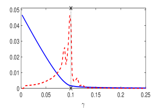
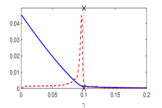
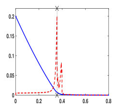
Fig. 1 shows two typical such plots of the function , where the left panel corresponds to a mixture of with (setting I) and in the right panel we have a mixture of Beta(1,10) and Uniform (setting II). We will use these two settings to illustrate our methodology in the rest of this section and also in Section 8.1.
Using the above heuristics, we can see that the “elbow” of the function should provide a good estimate of ; it is the point that has the maximum curvature, i.e., the point where the second derivative is maximal. We denote this estimator by . Notice that both the estimators and are derived from , as a function of , albeit they look at two different aspects of the function.
In the above plots we have used numerical methods to approximate the second derivative of (using the method of double differencing). We advocate plotting the function as varies between 0 and 1. In most cases, plots similar to Fig. 1 would immediately convey to the practitioner the most appropriate choice of . In some cases though, there can be multiple peaks in the second derivative, in which case some discretion on the part of the practitioner might be required. It must be noted that the idea of finding the point where the second derivative is large to detect an “elbow” or “knee” of a function is not uncommon; see e.g., Salvador and Chan (2004). However, in Section 8.2.4 and Appendix B, we show some simulation examples where fails to consistently estimate the “elbow” of
6 Estimation of the distribution function and its density
6.1 Estimation of
Let us assume for the rest of this section that (1) is identifiable, i.e., and . Thus . Once we have a consistent estimator (which may or may not be as discussed in the previous sections) of , a natural nonparametric estimator of is , defined as the minimiser of (3). In the following theorem we show that, indeed, is uniformly consistent for estimating . We also derive the rate of convergence of .
Theorem 8.
Suppose that . Then, as , Furthermore, if where , then Additionally, for as defined in (7), we have
for a function and a constant depending only on , and .
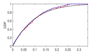
An immediate consequence of Theorem 8 is that as . Left panel of Fig. 2 shows our estimator along with the true for the same data set used in the right panel of Fig. 1.
6.2 Estimating the density of
Suppose now that has a density . Obtaining nonparametric estimators of can be difficult as it requires smoothing and usually involves the choice of tuning parameter(s) (e.g., smoothing bandwidths), and especially so in our set-up.
In this sub-section we describe a tuning parameter free approach to estimating , under the additional assumption that is non-increasing. The assumption that is non-increasing, i.e., is concave on its support, is natural in many situations (see Section 7 for an application in the multiple testing problem) and has been investigated by several authors, including Grenander (1956), Langaas et al. (2005) and Genovese and Wasserman (2004). Without loss of generality, we assume that is non-increasing on .
For a bounded function , let us represent the least concave majorant (LCM) of by . Thus, is the smallest concave function that lies above . Define . Note that is a valid CDF. We can now estimate by , where is the piece-wise constant function obtained by taking the left derivative of . In the following result we show that both and are consistent estimators of their population versions.
Theorem 9.
Assume that and that is concave on . If , then, as ,
| (12) |
Further, if for any , is continuous at , then,
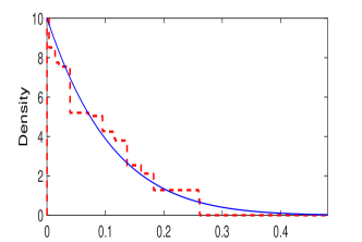
Computing and are straightforward, an application of the PAVA gives both the estimators; see e.g., Chapter 1 of Robertson et al. (1988). In Fig. 2 the left panel shows the LCM whereas the right panel shows its derivative along with the true density for the same data set used in the right panel of Fig. 1.
7 Multiple testing problem
The problem of estimating the proportion of false null hypotheses is of interest in situations where a large number of hypothesis tests are performed. Recently, various such situations have arisen in applications. One major motivation is in estimating the proportion of genes that are differentially expressed in deoxyribonucleic acid (DNA) microarray experiments. However, estimating the proportion of true null hypotheses is also of interest, for example, in functional magnetic resonance imaging (see Turkheimer et al. (2001)) and source detection in astrophysics (see Miller et al. (2001)).
Suppose that we wish to test null hypotheses on the basis of a data set . Let denote the (unobservable) binary variable that is if is true, and 1 otherwise, . We want a decision rule that will produce a decision of “null” or “non-null” for each of the cases. In their seminal work, Benjamini and Hochberg (1995) argued that an important quantity to control is the false discovery rate (FDR) and proposed a procedure with the property FDR , where is the user-defined level of the FDR procedure. When is significantly bigger than an estimate of can be used to yield a procedure with FDR approximately equal to and thus will result in an increased power. This is essentially the idea of the adapted control of FDR (see Benjamini and Hochberg (2000)). See Storey (2002), Black (2004), Langaas et al. (2005), Benjamini et al. (2006), and Donoho and Jin (2004) for a discussion on the importance of efficient estimation of and some proposed estimators.
Our method can be directly used to yield an estimator of that does not require the specification of any tuning parameter, as discussed in Section 5. We can also obtain a completely nonparametric estimator of , the distribution of the -values arising from the alternative hypotheses. Suppose that has a density and has a density . To keep the following discussion more general, we allow to be any known density, although in most multiple testing applications we will take to be Uniform. The local false discovery rate (LFDR) is defined as the function , where
and is the density of the observed -values. The estimation of the LFDR is important because it gives the probability that a particular null hypothesis is true given the observed -value for the test. The LFDR method can help us get easily interpretable thresholding methods for reporting the “interesting” cases (e.g., ). Obtaining good estimates of can be tricky as it involves the estimation of an unknown density, usually requiring smoothing techniques; see Section 5 of Efron (2010) for a discussion on estimation and interpretation of . From the discussion in Section 6.1, under the additional assumption that is non-increasing, we have a natural tuning parameter free estimator of the LFDR:
The assumption that is non-increasing, i.e., is concave, is quite natural – when the alternative hypothesis is true the -value is generally small – and has been investigated by several authors, including Genovese and Wasserman (2004) and Langaas et al. (2005).
8 Simulation
To investigate the finite sample performance of the estimators developed in this paper, we carry out several simulation experiments. We also compare the performance of these estimators with existing methods. The R language (R Development Core Team (2008)) codes used to implement our procedures are available at http://stat.columbia.edu/rohit/research.html.
8.1 Lower bounds for
| Setting I | Setting II | Setting I | Setting II | |||||||||
|---|---|---|---|---|---|---|---|---|---|---|---|---|
| 0 | 0.95 | 0.98 | 0.93 | 0.95 | 0.98 | 0.93 | 0.95 | 0.97 | 0.93 | 0.95 | 0.97 | 0.93 |
| 0.01 | 0.97 | 0.98 | 0.99 | 0.97 | 0.97 | 0.99 | 0.98 | 0.98 | 0.99 | 0.98 | 0.98 | 0.99 |
| 0.03 | 0.98 | 0.98 | 0.99 | 0.98 | 0.98 | 0.99 | 0.98 | 0.98 | 0.99 | 0.98 | 0.98 | 0.99 |
| 0.05 | 0.98 | 0.98 | 0.99 | 0.98 | 0.98 | 0.99 | 0.99 | 0.99 | 0.99 | 0.98 | 0.98 | 0.99 |
| 0.10 | 0.99 | 0.99 | 1.00 | 0.99 | 0.98 | 0.99 | 0.99 | 0.99 | 1.00 | 0.99 | 0.98 | 0.99 |
Although there has been some work on estimation of in the multiple testing setting, Meinshausen and Rice (2006) and Genovese and Wasserman (2004) are the only papers we found that discuss methodology for constructing lower confidence bounds for . These procedures are connected and the methods in Meinshausen and Rice (2006) are extensions of those proposed in Genovese and Wasserman (2004). The lower bounds proposed in both the papers approximately satisfy (11) and have the form where is a bounding sequence for the bounding function at level ; see Meinshausen and Rice (2006). Genovese and Wasserman (2004) use a constant bounding function, , with , whereas Meinshausen and Rice (2006) suggest a class of bounding functions but observe that the standard deviation-proportional bounding function has optimal properties among a large class of possible bounding functions. We use this bounding function and a bounding sequence suggested by the authors. We denote the lower bound proposed in Meinshausen and Rice (2006) by , the bound in Genovese and Wasserman (2004) by , and the lower bound discussed in Section 4 by . To be able to use the methods of Meinshausen and Rice (2006) and Genovese and Wasserman (2004) in setting I, introduced in Section 5, we transform the data such that is ; see Section 3.1 for the details.
We take and compare the performance of the three lower bounds in the two different simulation settings discussed in Section 5. For each setting we take the sample size to be and . We present the estimated coverage probabilities, obtained by averaging over independent replications, of the lower bounds for both settings in Table 1. We can immediately see from the table that the bounds are usually quite conservative. However, it is worth pointing out that when , our method has exact coverage, as discussed in Section 4. Also, the fact that our procedure is simple, easy to implement, and completely automated, makes it very attractive.
8.2 Estimation of
In this sub-section, we illustrate and compare the performance of different estimators of under two sampling scenarios. In scenario A, we proceed as in Langaas et al. (2005). Let , for , and assume that each and that are independent. We test versus for each . We set to zero for the true null hypotheses, whereas for the false null hypotheses, we draw from a symmetric bi-triangular density with parameters and ; see page 568 of Langaas et al. (2005) for the details. Let denote a realisation of and be the proportion of false null hypotheses. Let and . To test versus , we calculate a two-sided -value based on a one-sample -test, with , where is a -distributed random variable with degrees of freedom.
In scenario B, we generate independent random variables from and set for . The dependence structure of the ’s is determined by . For example, corresponds to the case where the ’s are i.i.d. standard normal. Let , for , where under the null, and under the alternative, is randomly generated from and , the sign of , is randomly generated from with equal probabilities. Here is a suitable constant that describes the simulation setting. Let be the proportion of true null hypotheses. Scenario B is inspired by the numerical studies in Cai and Jin (2010) and Jin (2008).
We use to denote the estimator proposed by Storey (2002) when bootstrapping is used to choose the required tuning parameter, and denote by the estimator when the value of the tuning parameter is fixed at Langaas et al. (2005) proposed an estimator that is tuning parameter free but crucially uses the known shape constraint of a convex and non-increasing ; we denote it by . We evaluate using the convest function in the R library limma. We also use the estimator proposed in Meinshausen and Rice (2006) for two bounding functions: and . For its implementation, we must choose a sequence going to zero as . Meinshausen and Rice (2006) did not specify any particular choice of but required the sequence satisfy some conditions. We choose and denote the estimators by when and by when (see Genovese and Wasserman (2004)). We also compare our results with , the estimator proposed in Efron (2007) using the central matching method, computed using the locfdr function in the R library locfdr. Jin (2008) and Cai and Jin (2010) propose estimators when the model is a mixture of Gaussian distributions; we denote the estimator proposed in Section 2.2 of Jin (2008) by and in Section 3.1 of Cai and Jin (2010) by Some of the competing methods require to be of a specific form (e.g., standard normal) in which case we transform the observed data suitably.
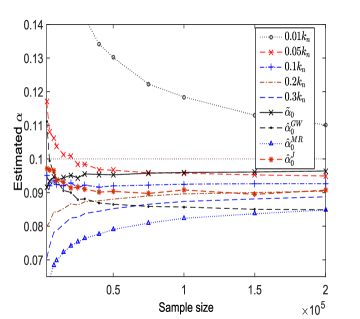
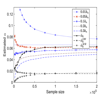
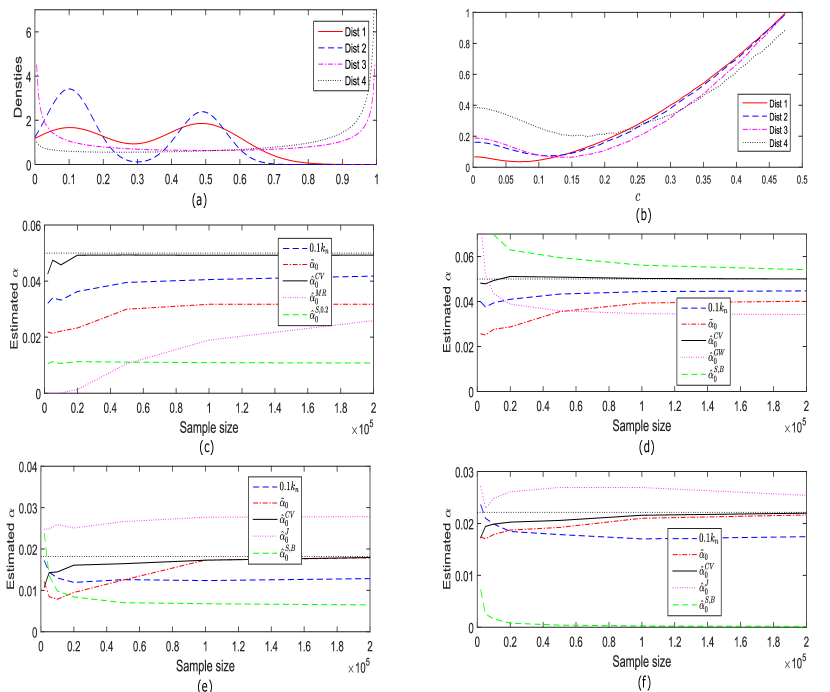
The estimator depends on the choice of and in the following we investigate a proper choice of . We take and evaluate the performance of for different values of , as increases, for scenarios A and B. The choice , for different values of , is suggested after extensive simulations. We also include , , , and in the comparison. For scenario A, we fix the sample size at and . For scenario B, we fix and In Fig. 3, we illustrate the effect of on estimation of as varies from to Recall that denotes the estimator proposed in Section 5. For both scenarios, the sample mean of the estimators of proposed in this paper converge to the true , as the sample size grows. The methods developed in this paper perform favorably in comparison to , , and Since, the choice of dictates the finite sample performance of we propose cross-validation to find an appropriate value of the tuning parameter.
| 0.10 | 0.13 | 0.15 | 0.13 | 0.00 | 0.01 | 0.09 | 0.14 | 0.05 | 0.16 | 0.36 |
| (1.00) | (1.79) | (0.83) | (1.00) | (0.88) | (1.41) | (1.50) | (5.32) | (1.20) | (3.70) | |
| 0.30 | 0.30 | 0.35 | 0.27 | 0.02 | 0.12 | 0.29 | 0.29 | 0.15 | 0.35 | 0.36 |
| (1.02) | (1.87) | (1.01) | (2.80) | (1.84) | (1.41) | (1.83) | (5.46) | (1.26) | (3.96) | |
| 0.50 | 0.48 | 0.51 | 0.46 | 0.18 | 0.26 | 0.47 | 0.49 | 0.26 | 0.55 | 0.35 |
| (1.09) | (1.9) | (1.12) | (3.29) | (2.46) | (1.49) | (1.91) | (5.73) | (1.34) | (3.80) | |
| 1.00 | 0.93 | 0.97 | 0.93 | 0.62 | 0.65 | 0.95 | 0.96 | 0.51 | 1.02 | 0.33 |
| (1.35) | (1.86) | (1.32) | (3.88) | (3.57) | (1.51) | (1.94) | (7.16) | (1.36) | (3.73) |
| 0.07 | 0.03 | 0.04 | 0.08 | 0.00 | 0.00 | 0.04 | 0.11 | 0.19 | 0.03 | 0.06 |
| (0.44) | (0.67) | (0.28) | (0.66) | (0.66) | (0.65) | (0.96) | (2.96) | (0.38) | (0.77) | |
| 0.20 | 0.14 | 0.18 | 0.16 | 0.00 | 0.01 | 0.08 | 0.28 | 0.55 | 0.07 | 0.05 |
| (0.73) | (0.79) | (0.62) | (1.98) | (1.89) | (2.25) | (1.33) | (4.41) | (1.26) | (1.28) | |
| 0.33 | 0.25 | 0.31 | 0.28 | 0.02 | 0.04 | 0.12 | 0.48 | 0.92 | 0.12 | 0.05 |
| (0.89) | (0.85) | (0.95) | (3.15) | (2.91) | (3.83) | (1.77) | (6.48) | (2.14) | (1.90) | |
| 0.66 | 0.55 | 0.62 | 0.58 | 0.12 | 0.14 | 0.23 | 0.95 | 1.83 | 0.23 | 0.05 |
| (1.21) | (1.00) | (1.48) | (5.38) | (5.25) | (7.73) | (3.04) | (11.98) | (4.34) | (3.84) |
8.2.1 Cross-validation
In this sub-section, we use instead of to simplify the notation. In the following we briefly describe our cross-validation procedure. For a -fold cross validation, we randomly partition the data into sets, say Let be the empirical CDF of the data in Let be the estimator defined in (7) using all data except those in and tuning parameter . Further, let be the estimator of as defined in Lemma 1 using and all data except those in Define the cross-validated estimator of as
| (13) |
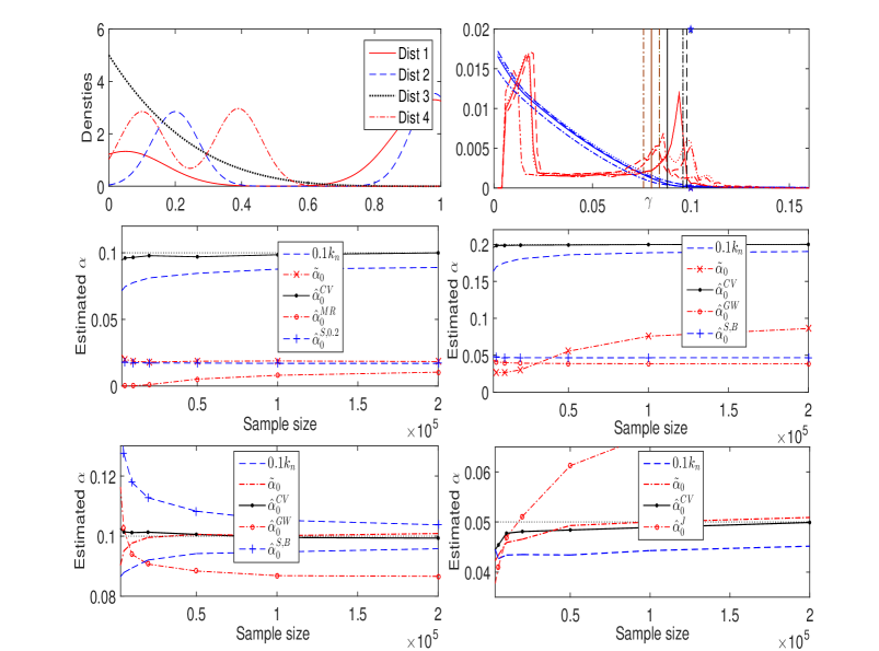
where In all simulations in this paper, we use and denote this estimator by see Section 7.10 of Hastie et al. (2009) for a more detailed study of cross-validation and a justification for . Fig. 4 illustrates the superior performance of across different simulation settings; also see Sections 8.2.2 and 8.2.4, and Appendix B
8.2.2 Performance under independence
In this sub-section, we take and compare the performance of the different estimators under the independence setting of scenarios A and B. In Tables 2 and 3, we give the mean and root mean squared error (RMSE) of the estimators over 5000 independent replications. For scenario A, we fix the sample size at and . For scenario B, we fix and By an application of Lemma 4, it is easy to see that in scenario A, the model is identifiable (i.e., ), while in scenario B, . For scenario A, the sample means of and for are comparable. However, the RMSEs of and are lower than those of and For scenario B, the sample means of and are comparable. In scenario B, the performances of and are not comparable to the estimators proposed in this paper, as and estimate while and estimate Note that fails to estimate because the underlying assumption inherent in their estimation procedure, that be non-increasing, does not hold. In scenario A, has the best performance among the different values of while in scenario B, has poor performance for all values of Furthermore, and perform poorly in both scenarios for all values of
8.2.3 Performance under dependence
The simulation settings of this sub-section are designed to investigate the effect of dependence on the performance of the estimators. For scenario A, we use the setting of Langaas et al. (2005). We take to be a block diagonal matrix with block size 100. Within blocks, the diagonal elements (i.e., variances) are set to 1 and the off-diagonal elements (within-block correlations) are set to . Outside of the blocks, all entries are set to 0. Tables 4 and 5 show that in both scenarios, none of the methods perform well for small values of However, in scenario A, the performances of and are comparable, for larger values of In scenario B, performs well for and . Observe that, as in the independence setting, and perform poorly in both scenarios for all values of
| 0.10 | 0.46 | 0.42 | 0.33 | 0.07 | 0.06 | 0.28 | 0.22 | 0.07 | 0.32 | 0.37 |
| (5.15) | (4.23) | (3.84) | (1.72) | (1.27) | (4.11) | (3.03) | (10.61) | (4.37) | (3.91) | |
| 0.30 | 0.52 | 0.53 | 0.41 | 0.14 | 0.17 | 0.65 | 0.34 | 0.15 | 0.49 | 0.39 |
| (3.80) | (3.64) | (3.59) | (2.72) | (1.90) | (6.58) | (3.25) | (10.35) | (4.30) | (4.31) | |
| 0.50 | 0.66 | 0.76 | 0.54 | 0.26 | 0.31 | 0.54 | 0.49 | 0.25 | 0.66 | 0.37 |
| (3.52) | (5.43) | (3.85) | (3.56) | (2.50) | (2.61) | (3.60) | (10.45) | (4.31) | (4.03) | |
| 1.00 | 1.06 | 1.13 | 0.97 | 0.68 | 0.69 | 1.15 | 0.97 | 0.53 | 1.11 | 0.36 |
| (3.09) | (3.92) | (4.00) | (4.15) | (3.54) | (6.01) | (3.61) | (10.55) | (4.13) | (3.99) |
| 0.07 | 0.29 | 0.38 | 0.17 | 0.04 | 0.05 | 0.26 | 0.20 | 0.21 | 0.13 | 0.22 |
| (2.92) | (3.70) | (1.62) | (1.02) | (1.36) | (3.71) | (2.80) | (9.87) | (1.75) | (2.22) | |
| 0.20 | 0.30 | 0.42 | 0.18 | 0.04 | 0.04 | 0.16 | 0.33 | 0.55 | 0.13 | 0.19 |
| (1.84) | (2.88) | (1.25) | (1.75) | (1.71) | (2.24) | (3.25) | (10.35) | (1.42) | (2.27) | |
| 0.33 | 0.38 | 0.52 | 0.20 | 0.06 | 0.06 | 0.17 | 0.50 | 0.93 | 0.16 | 0.18 |
| (1.54) | (2.74) | (1.89) | (2.83) | (2.73) | (3.51) | (3.71) | (11.52) | (2.03) | (2.59) | |
| 0.67 | 0.63 | 0.77 | 0.31 | 0.14 | 0.15 | 0.24 | 0.95 | 1.82 | 0.25 | 0.16 |
| (1.53) | (2.25) | (4.32) | (5.26) | (5.13) | (7.60) | (4.54) | (15.13) | (4.23) | (4.08) |
8.2.4 Comparing the performance of and
Although the heuristic estimator performs quite well in most of the simulation settings considered, there exists scenarios where can fail to consistently estimate . To illustrate this we consider four different CDFs and fix to be the uniform distribution on (see the top left plot of Fig. 4) and compare the performance of , , with the best performing competing estimators (in each setting).
We see that may fail to estimate the “elbow” of , as a function of , when has a multi-modal density (see the middle row of Fig. 4). Observe that and perform favorably compared to all competing estimators and in the two scenarios where fails to consistently estimate , all our competing estimators also fail.
The first two toy examples have been carefully constructed to demonstrate situations where the point of maximum curvature () is different from the “elbow” of the function; see the top right plot of Fig. 4 (also see Appendix B for further such examples).
8.2.5 Our recommendation
In this paper we study two estimators for . For , a proper choice of is important for good finite sample performance. We suggest using cross-validation to find the optimal tuning parameter . However, cross-validation can be computationally expensive. An attractive alternative in this situation is to use , which is easy to implement and has very good finite sample performance in most scenarios, especially with large sample sizes. We feel that a visual analysis of the plot of can be useful in checking the validity of as an estimator of the “elbow”, and thus for .
9 Real data analysis
9.1 Prostate data
Genetic expression levels for genes were obtained for men, normal control subjects and prostate cancer patients. Without going into the biology involved, the principal goal of the study was to discover a small number of “interesting” genes, that is, genes whose expression levels differ between the cancer and control patients. Such genes, once identified, might be further investigated for a causal link to prostate cancer development. The prostate data is a 6033 102 matrix having entries , , and with , for the normal controls, and , for the cancer patients. Let and be the averages of for the normal controls and for the cancer patients, respectively, for gene . The two-sample -statistic for testing significance of gene is where is an estimate of the standard error of , i.e.,
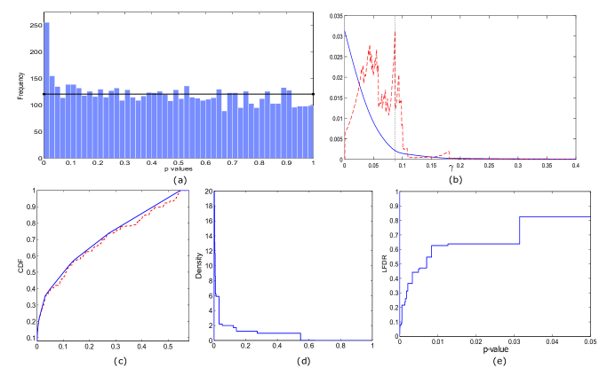
We work with the -values obtained from the 6033 two-sided -tests instead of the “-values” as then the distribution under the alternative will have a non-increasing density which we can estimate using the method developed in Section 6.1. Note that in our analysis we ignore the dependence of the -values, which is only a moderately risky assumption for the prostate data; see Chapters 2 and 8 of Efron (2010) for further analysis and justification. Fig. 5 show the plots of various quantities of interest, found using the methodology developed in Section 6.1 and Section 7, for the prostate data example. The 95% lower confidence bound for this data is found to be . In Table 6, we display estimates of based on the methods considered in this paper for the prostate data and the Carina data (described below).
9.2 Carina data – an application in astronomy
In this sub-section we analyse the radial velocity (RV) distribution of stars in Carina, a dwarf spheroidal (dSph) galaxy. The dSph galaxies are low luminosity galaxies that are companions of the Milky Way. The data have been obtained by Magellan and MMT telescopes (see Walker et al. (2007)) and consist of radial (line of sight) velocity measurements of stars from Carina, contaminated with Milky Way stars in the field of view. We would like to understand the distribution of the RV of stars in Carina. For the contaminating stars from the Milky Way in the field of view we assume a non-Gaussian velocity distribution that is known from the Besancon Milky Way model (Robin et al. (2003)), calculated along the line of sight to Carina.
| Data set | ||||||||||
|---|---|---|---|---|---|---|---|---|---|---|
| Prostate | 0.08 | 0.10 | 0.09 | 0.04 | 0.01 | 0.19 | 0.10 | 0.02 | 0.11 | 0.02 |
| Carina | 0.36 | 0.35 | 0.36 | 0.31 | 0.30 | 0.45 | 0.61 | 1.00 | 0.38 | NA |
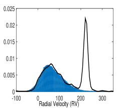
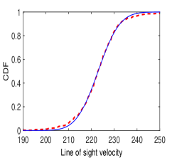
The 95% lower confidence bound for is found to be . The right panel of Fig. 6 shows the estimate of and the closest (in terms of minimising the distance) fitting Gaussian distribution. Astronomers usually assume the distribution of the RVs for these dSph galaxies to be Gaussian. Indeed we see that the estimated is close to a normal distribution (with mean and standard deviation ), although a formal test of this hypothesis is beyond the scope of the present paper. The estimate due to Cai and Jin (2010), , is greater than one, while Efron’s method (see Efron (2007)), implemented using the “locfdr” package in R, fails to estimate
10 Concluding remarks
In this paper we develop procedures for estimating the mixing proportion and the unknown distribution in a two component mixture model using ideas from shape restricted function estimation. We discuss the identifiability of the model and introduce an identifiable parameter , under minimal assumptions on the model. We propose an honest finite sample lower confidence bound of that is distribution-free. Two point estimators of , and , are studied. We prove that is a consistent estimator of and show that the rate of convergence of can be arbitrarily close to , for proper choices of . These proposed estimators crucially rely on , as a function of , whose plot provides useful insights about the nature of the problem and performance of the estimators.
We observe that the estimators of proposed in this paper have superior finite sample performance than most competing methods. In contrast to most previous work on this topic the results discussed in this paper hold true even when (1) is not identifiable. Under the assumption that (1) is identifiable, we can find an estimator of which is uniformly consistent. Furthermore, if is known to have a non-increasing density we can find a consistent estimator of . All these estimators are tuning parameter free and easily implementable.
We conclude this section by outlining some possible future research directions. Construction of two-sided confidence intervals for remains a hard problem as the asymptotic distribution of depends on the unknown . We are currently developing estimators of when we do not exactly know but only have an estimator of (e.g., we observe a second i.i.d. sample from ). Investigating consistent alternative ways of detecting the “elbow” of the function , as an estimator of , is an interesting future research direction. As we have observed in the astronomy application, formal goodness-of-fit tests for are important – they can guide the practitioner to use appropriate parametric models for further analysis – but are presently unknown. The -values in the prostate data example, considered in Section 9.1, can have slight dependence. Therefore, investigating the performance and properties of the methods introduced in this paper under appropriate dependence assumptions on is another important direction for future research.
Acknowledgements
We thank the Joint Editor, the Associate Editor, and five anonymous referees for their careful reading and constructive comments that lead to an improved version of the paper.
Appendix A Identifiability of
In this section we continue the discussion on the identifiability of . First, we give some remarks to illustrate Lemmas 3 and 4.
Remark 2.
We consider mixtures of Poisson and binomial distributions to illustrate Lemma 3. If is Poisson and is Poisson, then
By an application of Lemma 3, we have if then ; otherwise
In the case of a binomial mixture, i.e., and ,
Remark 3.
If is and is then it can be easily shown that the problem is identifiable if and only if . When the model is not identifiable, an application of Lemma 4 gives . Thus, increases to as tends to infinity. It should be noted that the problem is actually identifiable if we restrict ourselves to the parametric family of a two-component Gaussian mixture model.
Remark 4.
Now consider a mixture of exponential random variables, i.e., is and is , where is the distribution that has the density . In this case, the problem is identifiable if , as this implies the support of is a proper subset of the support of . But when , the problem is identifiable if and only if .
Remark 5.
It is also worth pointing out that even in cases where the problem is not identifiable the difference between the true mixing proportion and the estimand may be very small. Consider the hypothesis test versus for the model with test statistic . The density of the p-values under is
where is the sample size. Here , so the model is not identifiable. As is uniform, it can be easily verified that . However, as the value of decreases exponentially with , in many practical situations, where is not too small, the difference between and will be negligible.
In the following lemma, we try to find the relationship between and when is a general CDF.
Lemma 10.
Proof.
From the definition of and , we have and Thus from (1), we get
Now using the definition of , we see that If we write
it can easily seen that ; and similarly, . Then, we can find and as in Lemmas 3 and 4, respectively. Note that
where and are defined before Lemma 3 and we use the notion that . Hence, by (5) the result follows. ∎
Lemma 5 is now a corollary of this result.
Appendix B Performance comparison of and
In Figs. 7 and 8 we present further simulation experiments to investigate the finite sample performance of and across different simulation scenarios. In each setting we also include the performance of the best performing competing estimators discussed in Section 8.2.
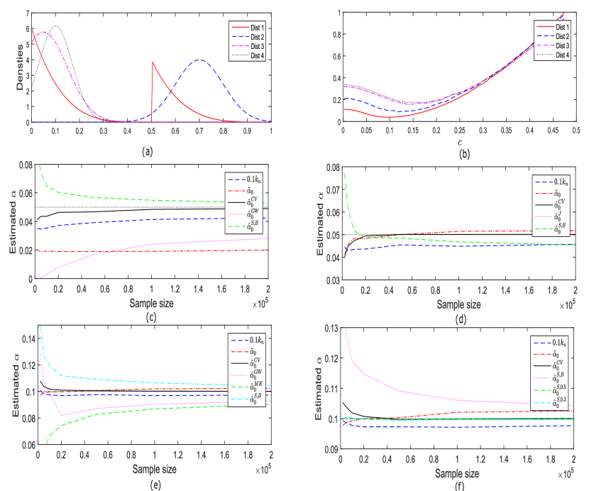
Appendix C Detection of sparse heterogeneous mixtures
In this section we draw a connection between the lower confidence bound developed in Section 4 and the Higher Criticism method of Donoho and Jin (2004) for detection of sparse heterogeneous mixtures. The detection of heterogeneity in sparse models arises in many applications, e.g., detection of a disease outbreak (see Kulldorff et al. (2005)) or early detection of bioweapons use (see Donoho and Jin (2004)). Generally, in large scale multiple testing problems, when the non-null effect is sparse it is important to detect the existence of non-null effects (see Cai et al. (2007)).
Donoho and Jin (2004) consider i.i.d. data from one of the two possible situations:
where and is such that is bounded away from 0. In Donoho and Jin (2004) the main focus is on testing , i.e., . We can test this hypothesis by rejecting when . The following lemma shows that indeed this yields a valid testing procedure for .
Theorem 10.
If , for , then and as .
Proof.
Note that is equivalent to which shows that
where is chosen as in Theorem 5. It is easy to see that is and , for , which shows that . It can be easily seen that . ∎
Appendix D Proofs of theorems and lemmas in the main paper
D.1 Proof of Lemma 2
From the definition of , we have
where the final equality follows from the fact that if , then will not be a sub-CDF.
To show that if and only if let us define . Note that , if and only if
However, it is easy to see that the last equality is true if and only if
D.2 Proof of Lemma 3
D.3 Proof of Lemma 4
From (5), we have
D.4 Proof of Theorem 1
Without loss of generality, we can assume that is the uniform distribution on and, for clarity, in the following we write instead of . Let us define
Since and for the first part of the theorem it is enough to show that Let us first show that . Suppose . We first show that is a non-decreasing function. For all , we have that
Let . Then,
since . However, as is continuous, and . Hence, we have
As and are CDFs, it is easy to see that ,
and is a right continuous function. Hence, for , is a CDF and thus, . We can similarly prove . Therefore, and .
Note that
where is the class of all CDFs. For the second part of theorem it is enough to show that
First note that
Thus, from the definition of we have
Therefore,
where . is a valid CDF as is non-decreasing.
D.5 Proof of Lemma 6
Letting , observe that
Also note that is a valid CDF for . As is defined as the function that minimises the distance of over all CDFs,
To prove the second part of the lemma, notice that for the result follows from above and the fact that as .
For , is not a valid CDF, by the definition of . Note that as , point-wise. So, for large enough , is not a valid CDF, whereas is always a CDF. Thus, converges to something positive.
D.6 Proof of Lemma 7
Assume that and . If , for , it is easy to observe from (2) that
Note that is a valid CDF, and thus from the definition of , we have
| (15) | |||||
where the last step follows from the triangle inequality. But as , the above inequality yields
Thus .
D.7 Proof of Theorem 2
We need to show that for any . Let us first show that
The statement is obviously true if . So let us assume that . Suppose , i.e., . Then by the definition of and the convexity of , we have (as is a convex set in with and ), and thus
| (16) |
But by (10) the left-hand side of (16) goes to a non-zero constant in probability. Hence, if ,
This completes the proof of the first part of the claim.
Now suppose that Then,
The first implication follows from the definition of , while the second implication is true by Lemma 6. The right-hand side of the last inequality is (asymptotically similar to) the Cramér–von Mises statistic for which the asymptotic distribution is well-known and thus if the result follows.
D.8 Proof of Lemma 8
D.9 Proof of Theorem 3
As the proof of this result is slightly involved we break it into a number of lemmas (whose proofs are provided later in this sub-section) and give the main arguments below.
We need to show that given any , we can find an and (depending on ) for which
Lemma 11.
If , then for any , , for large enough .
Finding an such that for large enough is more complicated. We start with some notation. Let be the class of all CDFs and be the Hilbert space . For a closed convex subset of and , we define the projection of onto as
| (18) |
where stands for the distance, i.e., if , then We define the tangent cone of at , as
| (19) |
For any and , let us define
For and we define the three quantities above and call them , , and respectively. Note that
| (20) |
where . To study the limiting behavior of we break it as the sum of and . The following two lemmas (proved in Sections D.9.2 and D.9.3 respectivley) give the asymptotic behavior of the two terms. The proof of Lemma 13 uses the functional delta method (cf. Theorem 20.8 of Van der Vaart (1998)) for the projection operator; see Theorem 1 of Fils-Villetard et al. (2008).
Lemma 12.
If then
Lemma 13.
If , then
where
and
| (21) |
Using (20), and the notation introduced in the above two lemmas we see that
| (22) |
However, (by Lemma 12) and (by Lemma 13). The result now follows from (22), by taking a large enough
D.9.1 Proof of Lemma 11
Note that
as , since . Therefore, the result holds for sufficiently large .
D.9.2 Proof of Lemma 12
It is enough to show that
| (23) |
since . Note that
For each positive integer and , we introduce the following classes of functions:
Let us also define
From the definition of the minimisers and , we see that
| (24) |
Observe that
where , denotes the empirical measure of the data, and denotes the usual empirical process. Similarly,
where . Thus, combining (23), (D.9.2) and the above two displays, we get, for any ,
| (25) |
The first term in the right hand side of (25) can be bounded above as
| (26) | |||||
where is an envelope for and is a constant. Note that to derive the last inequality, we have used the maximal inequality in Corollary (4.3) of Pollard (1989); the class is “manageable” in the sense of Pollard (1989) (as a consequence of equation (2.5) of Van de Geer (2000)).
To see that is an envelope for observe that for any ,
Hence,
As the two bounds are monotone, from the properties of isotonic estimators (see e.g., Theorem 1.3.4 of Robertson et al. (1988)), we can always find a version of such that
Therefore,
| (27) |
Thus, for ,
where the second inequality follows from (27). From the definition of and , we have , for all . As , for any given , there exists (depending on ) such that
| (28) |
for all sufficiently large .
Therefore, for any given and , we can make both and less than for large enough and , using the fact that and (28). Thus, by (26).
A similar analysis can be done for the second term of (25). The result now follows.
D.9.3 Proof of Lemma 13
Note that
However, a simplification yields
Since is , , and , we have
| (29) |
By applying the functional delta method (see Theorem 20.8 of Van der Vaart (1998)) for the projection operator (see Theorem 1 of Fils-Villetard et al. (2008)) to (29), we have
| (30) |
By combining (29) and (30), we have
| (31) |
The result now follows by applying the continuous mapping theorem to (31). We prove by contradiction. Suppose that , i.e., . Therefore, for some distribution function and , we have by the definition of . By the discussion leading to (5), it can be easily seen that is a sub-CDF, while is not (as that would contradict (5)). Therefore, and thus .
D.10 Proof of Theorem 4
The constant defined in the statement of the theorem can be explicitly expressed as
where
Let . Obviously,
By Lemma 11, we have that if . Now let . In this case the left hand side of the above display equals where . A simplification yields
| (32) |
since is ; see the proof of Lemma 13 (Section D.9.3) for the details. By applying the functional delta method (cf. Theorem 20.8 of Van der Vaart (1998)) for the projection operator (see Theorem 1 of Fils-Villetard et al. (2008)) to (32), we have
| (33) |
By the continuous mapping theorem, we get Hence, by Lemma 12,
D.11 Proof of Theorem 5
D.12 Proof of Theorem 6
It is enough to show that , where is the limiting distribution of the Cramér-von Mises statistic, a continuous distribution. As , it is enough to show that
| (34) |
We now prove (34). Observe that
| (35) |
where , denotes the empirical measure of the data, and denotes the usual empirical process. We will show that , which will prove (35).
For each positive integer , we introduce the following class of functions
Let us also define
From the definition of and , we have , for all . As , for any given , there exists (depending on ) such that
| (36) |
for all sufficiently large . Therefore, for any , using the same sequence of steps as in (26),
| (37) |
where is an envelope for and is a constant. Note that to derive the last inequality we have used the maximal inequality in Corollary (4.3) of Pollard (1989); the class is “manageable” in the sense of Pollard (1989) (as a consequence of equation (2.5) of Van de Geer (2000)).
D.13 Proof of Theorem 7
The random variable defined in the statement of the theorem can be explicitly expressed as
where is the -Brownian bridge.
By the same line of arguments as in the proof of Lemma 12 (see Section D.9.2), it can be easily seen that Moreover, by Donsker’s theorem,
By applying the functional delta method for the projection operator, in conjunction with the continuous mapping theorem to the previous display, we have
where , and are defined in (18), (19), and (21), respectively. Hence, by an application of the continuous mapping theorem, we have . The result now follows.
D.14 Proof of Lemma 9
Let . Then,
which shows that is a non-increasing function. To show that is convex, let and , for . Then, by (15) we have the desired result.
D.15 Proof of Theorem 8
The constant and the function defined in the statement of the theorem can be explicitly expressed as
and
where
Recall the notation of Section D.9. Note that from (2),
for all . Thus we can bound as follows:
where As both the upper and lower bounds are monotone, we can always find a version of such that
Therefore,
as , using the fact . Furthermore, if , where , it is easy to see that , as . Note that
Thus
Hence by an application of functional delta method for the projection operator, in conjunction with the continuous mapping theorem, we have
D.16 Proof of Theorem 9
Let . Then the function is concave on and majorises . Hence, for all , , as is the LCM of . Thus,
and therefore,
The second part of the result follows immediately from the lemma is page 330 of Robertson et al. (1988), and is similar to the result in Theorem 7.2.2 of that book.
References
- Anderson and Darling (1952) Anderson, T. W. and D. A. Darling (1952). Asymptotic theory of certain “goodness of fit” criteria based on stochastic processes. Ann. Math. Statistics 23, 193–212.
- Barlow et al. (1972) Barlow, R. E., D. J. Bartholomew, J. M. Bremner, and H. D. Brunk (1972). Statistical inference under order restrictions. The theory and application of isotonic regression. John Wiley & Sons, London-New York-Sydney. Wiley Series in Probability and Mathematical Statistics.
- Benjamini and Hochberg (1995) Benjamini, Y. and Y. Hochberg (1995). Controlling the false discovery rate: a practical and powerful approach to multiple testing. J. Roy. Statist. Soc. Ser. B 57(1), 289–300.
- Benjamini and Hochberg (2000) Benjamini, Y. and Y. Hochberg (2000). On the adaptive control of the false discovery rate in multiple testing with independent statistics. J. Educational and Behavioral Statistics 25, 60–83.
- Benjamini et al. (2006) Benjamini, Y., A. Krieger, and D. Yekutieli (2006). Adaptive linear step-up procedures that control the false discovery rate. Biometrika 93(3), 491–507.
- Bertsekas (2003) Bertsekas, D. P. (2003). Convex analysis and optimization. Athena Scientific, Belmont, MA. With Angelia Nedić and Asuman E. Ozdaglar.
- Black (2004) Black, M. A. (2004). A note on the adaptive control of false discovery rates. J. R. Stat. Soc. Ser. B Stat. Methodol. 66(2), 297–304.
- Bordes et al. (2006) Bordes, L., S. Mottelet, and P. Vandekerkhove (2006). Semiparametric estimation of a two-component mixture model. Ann. Statist. 34(3), 1204–1232.
- Cai et al. (2007) Cai, T., J. Jin, and M. G. Low (2007). Estimation and confidence sets for sparse normal mixtures. Ann. Statist. 35(6), 2421–2449.
- Cai and Jin (2010) Cai, T. T. and J. Jin (2010). Optimal rates of convergence for estimating the null density and proportion of nonnull effects in large-scale multiple testing. Ann. Statist. 38(1), 100–145.
- Celisse and Robin (2010) Celisse, A. and S. Robin (2010). A cross-validation based estimation of the proportion of true null hypotheses. J. Statist. Planng. Inf. 140(11), 3132–3147.
- Cohen (1967) Cohen, A. C. (1967). Estimation in mixtures of two normal distributions. Technometrics 9, 15–28.
- Day (1969) Day, N. E. (1969). Estimating the components of a mixture of normal distributions. Biometrika 56, 463–474.
- Donoho and Jin (2004) Donoho, D. and J. Jin (2004). Higher criticism for detecting sparse heterogeneous mixtures. Ann. Statist. 32(3), 962–994.
- Efron (2007) Efron, B. (2007). Size, power and false discovery rates. Ann. Statist. 35(4), 1351–1377.
- Efron (2010) Efron, B. (2010). Large-scale inference, Volume 1 of Institute of Mathematical Statistics Monographs. Cambridge: Cambridge University Press. Empirical Bayes methods for estimation, testing, and prediction.
- Feller (1971) Feller, W. (1971). An introduction to probability theory and its applications. Vol. II. Second edition. John Wiley & Sons, Inc., New York-London-Sydney.
- Fils-Villetard et al. (2008) Fils-Villetard, A., A. Guillou, and J. Segers (2008). Projection estimators of Pickands dependence functions. Canad. J. Statist. 36(3), 369–382.
- Genovese and Wasserman (2004) Genovese, C. and L. Wasserman (2004). A stochastic process approach to false discovery control. Ann. Statist. 32(3), 1035–1061.
- Grenander (1956) Grenander, U. (1956). On the theory of mortality measurement. I. Skand. Aktuarietidskr. 39, 70–96.
- Grotzinger and Witzgall (1984) Grotzinger, S. J. and C. Witzgall (1984). Projections onto order simplexes. Appl. Math. Optim. 12(3), 247–270.
- Hastie et al. (2009) Hastie, T., R. Tibshirani, J. Friedman, T. Hastie, J. Friedman, and R. Tibshirani (2009). The elements of statistical learning, Volume 2. Springer.
- Hengartner and Stark (1995) Hengartner, N. W. and P. B. Stark (1995). Finite-sample confidence envelopes for shape-restricted densities. Ann. Statist. 23(2), 525–550.
- Hunter et al. (2007) Hunter, D. R., S. Wang, and T. P. Hettmansperger (2007). Inference for mixtures of symmetric distributions. Ann. Statist. 35(1), 224–251.
- Jin (2008) Jin, J. (2008). Proportion of non-zero normal means: universal oracle equivalences and uniformly consistent estimators. J. R. Stat. Soc. Ser. B Stat. Methodol. 70(3), 461–493.
- Kulldorff et al. (2005) Kulldorff, M., J. Heffernan, R. Hartman, R. Assuncao, and F. Mostashari (2005). A space-time permutation scan statistic for disease outbreak detection. PLoS Med. 2(3), e59.
- Langaas et al. (2005) Langaas, M., B. H. Lindqvist, and E. Ferkingstad (2005). Estimating the proportion of true null hypotheses, with application to DNA microarray data. J. R. Stat. Soc. Ser. B Stat. Methodol. 67(4), 555–572.
- Lindsay (1983) Lindsay, B. G. (1983). The geometry of mixture likelihoods: a general theory. Ann. Statist. 11(1), 86–94.
- Lindsay (1995) Lindsay, B. G. (1995). Mixture models: Theory, geometry and applications. NSF-CBMS Regional Conference Series in Probability and Statistics 5, 1–163.
- Lindsay and Basak (1993) Lindsay, B. G. and P. Basak (1993). Multivariate normal mixtures: a fast consistent method of moments. J. Amer. Statist. Assoc. 88(422), 468–476.
- Lyons (2008) Lyons, L. (2008). Open statistical issues in particle physics. Ann. Appl. Stat. 2(3), 887–915.
- McLachlan and Peel (2000) McLachlan, G. and D. Peel (2000). Finite mixture models. Wiley Series in Probability and Statistics: Applied Probability and Statistics. Wiley-Interscience, New York.
- Meinshausen and Bühlmann (2005) Meinshausen, N. and P. Bühlmann (2005). Lower bounds for the number of false null hypotheses for multiple testing of associations under general dependence structures. Biometrika 92(4), 893–907.
- Meinshausen and Rice (2006) Meinshausen, N. and J. Rice (2006). Estimating the proportion of false null hypotheses among a large number of independently tested hypotheses. Ann. Statist. 34(1), 373–393.
- Miller et al. (2001) Miller, C. J., C. Genovese, R. C. Nichol, L. Wasserman, A. Connolly, D. Reichart, A. Hopkins, and A. Schneider, J.and Moore (2001). Controlling the false-discovery rate in astrophysical data analysis. Astron. J. 122(6), 3492––3505.
- Nguyen and Matias (2013) Nguyen, V. H. and C. Matias (2013). On efficient estimators of the proportion of true null hypotheses in a multiple testing setup. arXiv:1205.4097.
- Parzen (1960) Parzen, E. (1960). Modern probability theory and its applications. John Wiley & Sons, Incorporated.
- Pollard (1989) Pollard, D. (1989). Asymptotics via empirical processes. Statist. Sci. 4(4), 341–366. With comments and a rejoinder by the author.
- Quandt and Ramsey (1978) Quandt, R. E. and J. B. Ramsey (1978). Estimating mixtures of normal distributions and switching regressions. J. Amer. Statist. Assoc. 73(364), 730–752. With comments and a rejoinder by the authors.
- R Development Core Team (2008) R Development Core Team (2008). R: A Language and Environment for Statistical Computing. Vienna, Austria: R Foundation for Statistical Computing. ISBN 3-900051-07-0.
- Robertson et al. (1988) Robertson, T., F. T. Wright, and R. L. Dykstra (1988). Order restricted statistical inference. Wiley Series in Probability and Mathematical Statistics: Probability and Mathematical Statistics. Chichester: John Wiley & Sons Ltd.
- Robin et al. (2003) Robin, A. C., C. Reylé, S. Derrière, and S. Picaud (2003). A synthetic view on structure and evolution of the milky way. Astronomy and Astrophysics 409(1), 523–540.
- Robin et al. (2007) Robin, S., A. Bar-Hen, J.-J. Daudin, and L. Pierre (2007). A semi-parametric approach for mixture models: application to local false discovery rate estimation. Comput. Statist. Data Anal. 51(12), 5483–5493.
- Salvador and Chan (2004) Salvador, S. and P. Chan (2004). Determining the number of clusters/segments in hierarchical clustering/segmentation algorithms. Proc. 16th IEEE Intl. Conf. on Tools with AI 25, 576–584.
- Storey (2002) Storey, J. D. (2002). A direct approach to false discovery rates. J. R. Stat. Soc. Ser. B Stat. Methodol. 64(3), 479–498.
- Swanepoel (1999) Swanepoel, J. W. H. (1999). The limiting behavior of a modified maximal symmetric -spacing with applications. Ann. Statist. 27(1), 24–35.
- Turkheimer et al. (2001) Turkheimer, F., C. Smith, and K. Schmidt (2001). Estimation of the number of “true” null hypotheses in multivariate analysis of neuroimaging data. NeuroImage 13(5), 920–930.
- Van de Geer (2000) Van de Geer, S. A. (2000). Applications of empirical process theory, Volume 6 of Cambridge Series in Statistical and Probabilistic Mathematics. Cambridge: Cambridge University Press.
- Van der Vaart (1998) Van der Vaart, A. W. (1998). Asymptotic statistics, Volume 3 of Cambridge Series in Statistical and Probabilistic Mathematics. Cambridge: Cambridge University Press.
- Walker et al. (2009) Walker, M., M. Mateo, E. Olszewski, B. Sen, and M. Woodroofe (2009). Clean kinematic samples in dwarf spheroidals: An algorithm for evaluating membership and estimating distribution parameters when contamination is present. The Astronomical Journal 137, 3109.
- Walker et al. (2007) Walker, M. G., M. Mateo, E. W. Olszewski, O. Y. Gnedin, X. Wang, B. Sen, and M. Woodroofe (2007). Velocity dispersion profiles of seven dwarf spheroidal galaxies. Astrophysical J. 667(1), L53–L56.
- Walther (2001) Walther, G. (2001). Multiscale maximum likelihood analysis of a semiparametric model, with applications. Ann. Statist. 29(5), 1297–1319.
- Walther (2002) Walther, G. (2002). Detecting the presence of mixing with multiscale maximum likelihood. J. Amer. Statist. Assoc. 97(458), 508–513.