Finding low-energy conformations of lattice protein models by quantum annealing

Lattice protein folding models are a cornerstone of computational biophysics S̆ali, Shakhnovich, and Karplus (1994). Although these models are a coarse grained representation, they provide useful insight into the energy landscape of natural proteins Pande (2010); Dill et al. (2008); Mirny and Shakhnovich (2001); Pande, Grosberg, and Tanaka (2000); Kolinski and Skolnick (1996); Shakhnovich (1994). Finding low-energy three-dimensional structures is an intractable problem Berger and Leighton (1998); Crescenzi et al. (1998); Hart and Istrail (1997) even in the simplest model, the Hydrophobic-Polar (HP) model. Exhaustive search of all possible global minima is limited to sequences in the tens of amino acids Yue and Dill (1995). Description of protein-like properties are more accurately described by generalized models, such as the one proposed by Miyazawa and Jernigan Miyazawa and Jernigan (1996) (MJ), which explicitly take into account the unique interactions among all 20 amino acids. There is theoretical Amara, Hsu, and Straub (1993); Finnila et al. (1994); Kadowaki and Nishimori (1998); Farhi et al. (2001); Santoro et al. (2002) and experimental Brooke et al. (1999) evidence of the advantage of solving classical optimization problems using quantum annealing Finnila et al. (1994); Kadowaki and Nishimori (1998); Santoro and Tosatti (2006); Das and Chakrabarti (2008) over its classical analogue (simulated annealing Kirkpatrick, Gelatt, and Vecchi (1983)). In this report, we present a benchmark implementation of quantum annealing for a biophysical problem (six different experiments up to 81 superconducting quantum bits). Although the cases presented here can be solved in a classical computer, we present the first implementation of lattice protein folding on a quantum device under the Miyazawa-Jernigan model. This paves the way towards studying optimization problems in biophysics and statistical mechanics using quantum devices.

The search for more efficient optimization algorithms is an important endeavor with prevalence on many disciplines ranging from the social sciences to the physical and natural sciences. Belonging to the latter, the protein folding problem Dill et al. (2008); Mirny and Shakhnovich (2001); Kolinski and Skolnick (1996); Pande, Grosberg, and Tanaka (2000) consists of finding the lowest free-energy configuration or, equivalently, the native structure of a protein given its amino acid sequence. Knowing how proteins fold elucidate their three-dimensional structure-function relationship which is crucial to the understanding of enzymes and for the treatment of misfolded-protein diseases such as Alzheimer’s, Huntington’s, and Parkinson’s disease. Due to the high computational cost of modeling proteins in atomistic detail Bohannon (2005); Shaw et al. (2010), coarse-grained descriptions of the protein folding problem, such as those found in lattice models, provide valuable insight about the folding mechanisms Kolinski and Skolnick (1996); Pande, Grosberg, and Tanaka (2000); Mirny and Shakhnovich (2001); Pande (2010); Li et al. (2010).

Harnessing quantum-mechanical effects to speed up the solving of classical optimization problems is at the heart of quantum annealing algorithms (QA) Finnila et al. (1994); Kadowaki and Nishimori (1998); Santoro and Tosatti (2006); Das and Chakrabarti (2008). In QA, quantum mechanical tunneling allows for more efficient exploration of difficult potential energy landscapes such as that of classical spin-glass problems. In our implementation of lattice folding, quantum fluctuations (tunneling) occurs between states representing different model protein conformations or folds.

The theoretical challenge is to efficiently map the hard computational problem of interest (e.g., lattice folding) to a classical spin-glass Hamiltonian: such mapping requiring a polynomial number of quantum bits (qubits) with the size of the problem (protein length) is described elsewhere Perdomo et al. (2008). Here we present a new mapping which, due to its exponential scaling with problem size, is not intended for large instances. The proposed mapping employs very few qubits for small problem instances, making it ideal for this first experimental demonstration and implementation on current quantum devices Johnson et al. (2011). A combination of the existing polynomial mapping Perdomo et al. (2008) and more advanced quantum devices would allow for the simulation of much larger instances of lattice folding and other related optimization problems.

Solving arbitrary problem instances requires a programmable quantum device to implement the corresponding classical Hamiltonian. We employ quantum annealing on the programmable device to obtain low-energy conformations of the protein model. We emphasize that nothing quantum mechanical is implied about the protein or its folding process; rather quantum fluctuations are a tool we use to solve the optimization problem.

The QA protocol performed here is also known as adiabatic quantum computation (AQC) Farhi et al. (2000, 2001). Of all the quantum-computational models, AQC is perhaps the most naturally suited for studying and solving optimization problems Farhi et al. (2001); Hogg (2003). For the experiments presented here, the small finite temperature of the superconducting device is enough to make the process less coherent than the original formulation of AQC, where the theoretical limit of zero temperature and quasi-adiabaticity are usually assumed Farhi et al. (2000, 2001). As we show in the discussion, numerical simulations including these unavoidable environmental effects accurately reproduce our experimental results.

Experimental implementations of QA or AQC are limited either by the number of qubits available in state-of-the-art quantum devices or by the programmability required to fulfill the problem specification. For example, the first realization of AQC was performed on a three-qubit NMR quantum device Steffen et al. (2003) and newer NMR implementations involve four qubit experiments Xu et al. (2011). Other experimental realizations of spin systems have been based on measuring bulk magnetization properties of the systems in which there is no control over the individual spins and the couplings among them Brooke et al. (1999); Wernsdorfer (2010). Quantum architectures using superconducting qubits  Vion et al. (2002); You and Nori (2005); Lupascu et al. (2007); Hofheinz et al. (2009); DiCarlo et al. (2009); Neeley et al. (2010); DiCarlo et al. (2010); Kaminsky, Lloyd, and Orlando (2004) offer promising device scalability while maintaining the ability to control individual qubits and the strength of their interaction couplings. During the preparation of this manuscript, an 84-qubit experimental determination of Ramsey numbers with quantum annealing was performed Bian et al. (2012), underscoring the programmable capabilities of the device for problems with over 80 qubits. In this letter, we present a quantum annealing experimental implementation of lattice protein models with general (Miyazawa-Jernigan Miyazawa and Jernigan (1996)) interactions among the amino acids. Even though the cases presented here still can be solved on a classical computer by exact enumeration (the six-amino acid problem has only 40 possible configurations), it is remarkable that the device anneals to the ground state of a search space of $2^{81}$ possible computational outcomes. This study provides a proof-of-principle that optimization of biophysical problems such as protein folding can be studied using quantum mechanical devices.

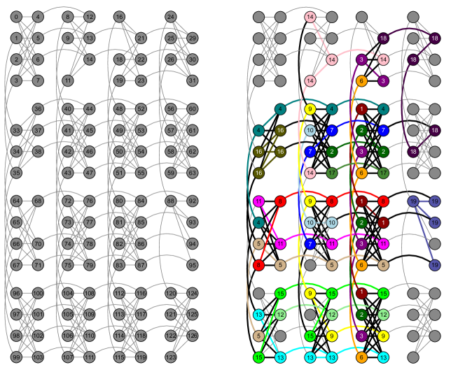
The quantum hardware employed consists of 16 units of a recently characterized eight-qubit unit cell Harris et al. (2010); Johnson et al. (2011). Post-fabrication characterization determined that only 115 qubits out of the 128 qubit array can be reliably used for computation (see Fig. 1). The array of coupled superconducting flux qubits is, effectively, an artificial Ising spin system with programmable spin-spin couplings and transverse magnetic fields. It is designed to solve instances of the following (NP-hard Barahona (1982)) classical optimization problem: Given a set of local longitudinal fields $\{h_{i}\}$ and an interaction matrix $\{J_{ij}\}$, find the assignment $\mathbf{s^{*}}=s^{*}_{1}s^{*}_{2}\cdots s^{*}_{N}$, that minimizes the objective function $E(\mathbf{s})$, where,

$$E(\mathbf{s})=\sum_{1\leq i\leq N}h_{i}s_{i}+\sum_{1\leq i<j\leq N}J_{ij}s_{i}s_{j},$$ (1)

$\lvert h_{i}\rvert\leq 1$, $\lvert J_{ij}\rvert\leq 1$, and $s_{i}\in\{+1,-1\}$.

Finding the optimal $\mathbf{s^{*}}$ is equivalent to finding the ground state of the corresponding Ising classical Hamiltonian,

$$H_{p}=\sum^{N}_{1\leq i\leq N}h_{i}\sigma_{i}^{z}+\sum^{N}_{1\leq i<j\leq N}J_{ij}\sigma_{i}^{z}\sigma_{j}^{z}$$ (2)

where $\sigma_{i}^{z}$ are Pauli matrices acting on the $i$th spin.

Experimentally, the time-dependent quantum Hamiltonian implemented in the superconducting-qubit array is given by,

$$H(\tau)=A(\tau)H_{b}+B(\tau)H_{p},\quad\quad\tau=t/t_{run},$$ (3)

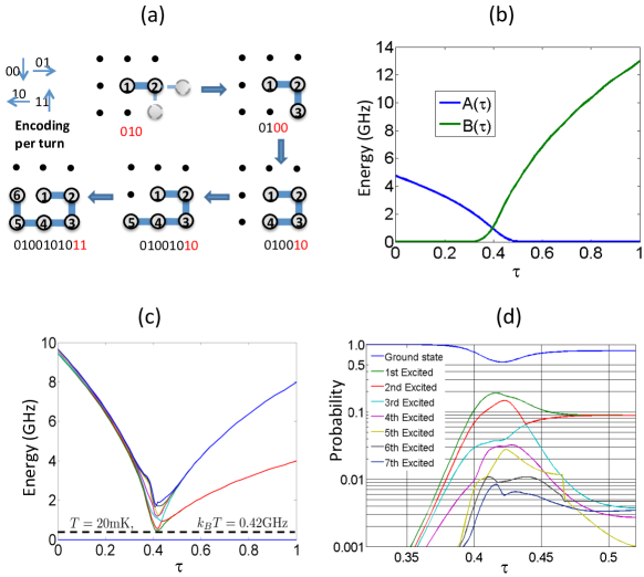
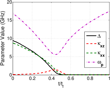
with $H_{b}=-\sum_{i}\sigma^{x}_{i}$ responsible for quantum tunneling among the localized classical states, which correspond to the eigenstates of $H_{p}$ (the computational basis). The time-dependent functions $A(\tau)$ and $B(\tau)$ are such that $A(0)\gg B(0)$ and $A(1)\ll B(1)$; in Fig. 2(b), we plot these functions as implemented in the experiment. $t_{run}$ denotes the time elapsed between the preparation of the initial state and the measurement.

QA exploits the adiabatic theorem of quantum mechanics, which states that a quantum system initialized in the ground state of a time-dependent Hamiltonian remains in the instantaneous ground state, as long as it is driven sufficiently slowly. Since the ground state of $H_{p}$ encodes the solution to the optimization problem, the idea behind QA is to adiabatically prepare this ground state by initializing the quantum system in the easy-to-prepare ground state of $H_{b}$, which corresponds to a superposition of all $2^{N}$ states of the computational basis. The system is driven slowly to the problem Hamiltonian, $H(\tau=1)\approx H_{p}$. Deviations from the ground-state are expected due to deviations from adiabaticity, as well as thermal noise and imperfections in the implementation of the Hamiltonian.

The first challenge of the experimental implementation is to map the computational problem of interest into the binary quadratic expression (Eq. 2), which we outline next. In lattice folding, the sequence of amino acids defining the protein is viewed as a sequence of beads (amino acids) connected by strings (peptide bonds). This bead chain occupies points on a two- or three-dimensional lattice. A valid configuration is a self-avoiding walk on the lattice and its energy is calculated from the sum of interaction energies between nearest non-bonded neighbors on the lattice. By the thermodynamic hypothesis of protein folding Anfinsen (1973), the global minimum of the free-energy function is conjectured to be the native functional conformation of the protein.

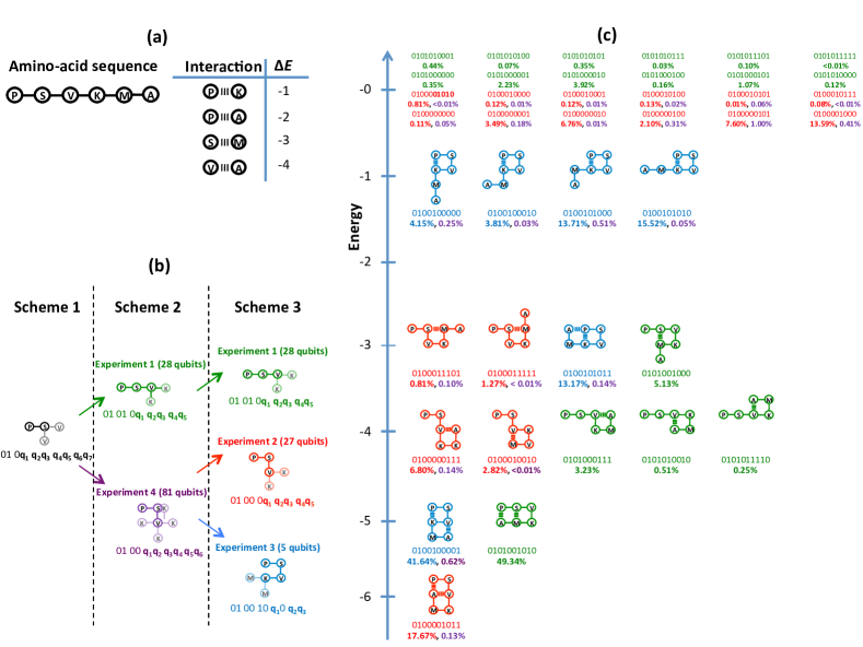
The hydrophobic-polar (HP) model is one of the simplest possible models for lattice folding Lau and Dill (1989). In this model, the amino acids are classified into two groups, hydrophobic (H) and polar (P). To describe real protein energy landscapes a more elaborate description needs to be considered, such as the Mijazawa-Jernigan (MJ) model Miyazawa and Jernigan (1996) which assigns the interaction energies for pairwise interactions among all twenty amino acids. The formulation we used is general enough to take into account arbitrary interaction matrices for lattice models in two and three dimensions Perdomo-Ortiz, O’Gorman, and Aspuru-Guzik (2011). In particular, we solved a MJ model in 2D, the six amino-acid sequence of Proline-Serine-Valine-Lysine-Methionine-Alanine (PSVKMA in the one-letter amino-acid sequence notation). We solved the problem under two different experimental schemes (see Schemes 2 and 3 in Fig. 3), each requiring a different number of resources. Solving the problem in one proposed experimental realization (Scheme 1) requires more resources than the number of qubits available (115 qubits) in the device. Scheme 2 and 3 are examples of the divide-and-conquer strategy, in which one partitions the problem in smaller instances and combines the independent set of results, thereby obtaining the same solution for the intractable problem. In the SI section, we complement these four MJ related experiments with two small tetrapeptide instances (effectively HP model instances) for a total of six different problem Hamiltonians. We used the largest of these two instances (an 8 qubit experiment) for direct theoretical simulation of the annealing dynamics of the device. The results from our experiment and the theoretical model, which does not use any adjustable parameters (all are extracted experimentally from the device), are in excellent agreement (see panel (b), Fig. 2 of the SI material).

To represent each of the possible $N$-amino-acid configurations (folds) in the lattice, we encode the direction of each successive bond between amino acids; thus, for every $N$-bead sequence we need to specify $N-1$ turns corresponding to the number of bonds. For the case of a two dimensional lattice, a bond can take any of four possible directions; therefore, two bits per bond are required to uniquely determine a direction. More specifically, if a bond points upwards, we write “11”. If it points downwards, leftwards or rightwards, we write “00”, “10”, or “01” respectively. Fixing the direction of the first bond reduces the description of any $N$-bead fold to $\ell=2(N-2)$ binary variables, without loss of generality. As shown in Fig. 2(a), in the absence of external constraints other than those imposed by the primary amino acid sequence (see SI for an example with external constraints), we can fix the third binary variable to “0”, forcing the third amino acid to go either straight or downward and reducing the number of needed variables to $\ell=2N-5$. This constraint reduces the solution space by removing conformations which are degenerate due to rotational symmetry. Thus, a particular fold is uniquely defined by,

$$\bm{q}=\underbrace{01}_{turn1}\underbrace{0q_{1}}_{turn2}\underbrace{q_{2}q_{3}}_{turn3}\cdots\underbrace{q_{2N-6}q_{2N-5}}_{turn(N-1)}$$ (4)

An example of this encoding for a six-amino-acid sequence is represented in Fig. 2(a).

Using this mapping to translate between the amino acid chain in the lattice and the $2(N-1)$ string of bits, we constructed the energy function $E(\bm{q})$ in which $\bm{q}$ denotes the remaining $2N-5$ binary variables. Additionally, we penalized folds which exhibit two amino acids on top of each other, to favor self-avoiding walk configurations. The energy penalty chosen for each problem was sufficient to push the energy of invalid folds outside of the energy range of valid configurations (those with $E\leq 0$). Finally, we took into account the interaction energy among the different amino acids. A detailed construction of our energy function for the general case of $N$ amino acids with arbitrary interactions is given elsewhere Perdomo-Ortiz, O’Gorman, and Aspuru-Guzik (2011).

The experiment consists of the following steps: a) construction of the energy function to be minimized in terms of the turn encoding; b) reduction of the energy expression to a two-body Hamiltonian; and finally, c) embedding in the device. These last two steps need additional resources as explained below. We will focus on the simplest example (Experiment 3, Fig. 3) to show the procedure in detail. The embeddings for the other five experiments are provided in the SI material. The energy function for Experiment 3, containing the contributions due to on-site penalties for overlapping amino acids, and pairwise interactions between amino acids is,

$$E(\bm{q})\equiv E^{cubic}_{exp3}=-1-4q_{3}+9q_{1}q_{3}+9q_{2}q_{3}-16q_{1}q_{2}q_{3}$$ (5)

where $q_{1}0$ ($q_{2}q_{3}$) encodes the orientation of the fourth (fifth) bond (see Fig. 3). From Eq. 5 one can verify by substitution that the eight possible three-bit-variable assignments provide the desired energy landscape: the six conformations with $E\leq 0$ shown in blue in Fig. 3.

Eq. 5 describes the energy landscape of configurations but it is not quite ready for the device. Experimentally, we can specify up to two-body spin interactions, $\sigma^{z}_{i}\sigma^{z}_{j}$, and therefore, we need to convert this cubic energy function (Eq. 5) into a quadratic form resembling Eq. 1 (see SI for details). The resulting expression is

$$\begin{split}H^{\text{unembedded}}_{p}&=(7\sigma^{z}_{1}+9\sigma^{z}_{2}+8\sigma^{z}_{3}-20\sigma^{z}_{4}+9\sigma^{z}_{1}\sigma^{z}_{3}+9\sigma^{z}_{2}\sigma^{z}_{3}\\ &-16\sigma^{z}_{1}\sigma^{z}_{4}-18\sigma^{z}_{2}\sigma^{z}_{4}-18\sigma^{z}_{3}\sigma^{z}_{4})/4\end{split}$$ (6)

where the original binary variables and spin operators are related by $q_{i}\rightarrow(1-\sigma^{z}_{i})/2$. Experimental measurements of $\sigma^{z}_{i}$ yield $s_{i}=+1$ ($s_{i}=-1$) corresponding to $q_{i}=0$ ($q_{i}=1$). Since $q_{i}=(1-s_{i})/2$, measurement of $s_{1}$, $s_{2}$, and $s_{3}$ allows us to reconstruct the bit string $q_{1}0q_{2}q_{3}$ which encodes the desired fold.

One ancilla variable was added during the transformation of the three-variable cubic Hamiltonian into this quadratic four-variable expression. The meaning of the original variables $s_{1}$, $s_{2}$, and $s_{3}$ remains the same, allowing for the reconstruction of the folds. The energy of this four-variable expression will not change as long as the measurements of $\sigma^{z}_{1}$ through $\sigma^{z}_{4}$ result in values for $q_{1}q_{2}q_{3}q_{4}$ satisfying $q_{4}=q_{2}q_{3}$. This transformation ensures an energy penalty whenever this condition is violated.

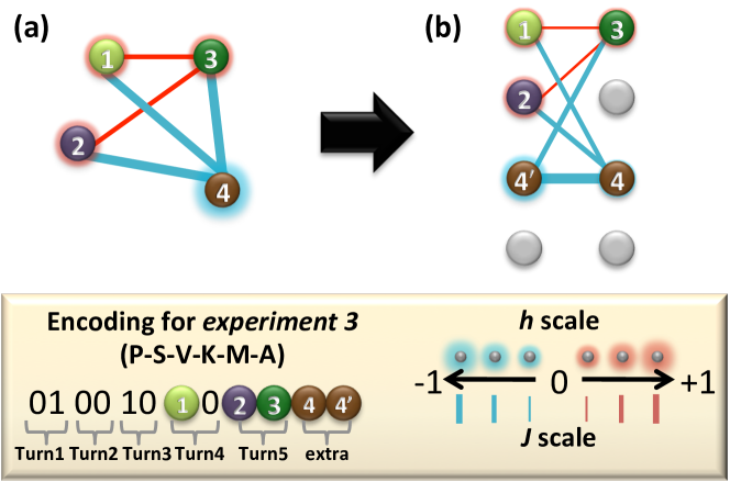
The architecture of the chip lacks sufficient connectivity between the superconducting rings for a one-to-one assignment of variables to qubits (see Fig. 4). To satisfy the connectivity requirements of the four-variable energy function, the couplings of one of the most connected variables, $q_{4}$, were fulfilled by duplicating this variable inside the device such that $q_{4}\rightarrow q_{4}$ and $q_{4^{\prime}}$. In the form of Eq. 2 the final expression representing the energy function of Experiment 3 is given by,

$$\begin{split}H_{p}&=(7\sigma^{z}_{2}\sigma^{z}_{1}+9\sigma^{z}_{2}+8\sigma^{z}_{3}+9\sigma^{z}_{1}\sigma^{z}_{3}+9\sigma^{z}_{2}\sigma^{z}_{4^{\prime}}-2\sigma^{z}_{4^{\prime}}-16\sigma^{z}_{1}\sigma^{z}_{4^{\prime}}\\ &-18\sigma^{z}_{2}\sigma^{z}_{4^{\prime}}-18\sigma^{z}_{4^{\prime\prime}}-18\sigma^{z}_{3}\sigma^{z}_{4^{\prime\prime}}-36\sigma^{z}_{4^{\prime\prime}}\sigma^{z}_{4^{\prime\prime}})/36\end{split}$$ (7)

This expression satisfies all requirements for the problem Hamiltonian (Eq. 3), the completion of which allows for the measurement of the energetic minimum conformation of this small peptide instance. The embedding of Eq. 7 into the hardware is shown in Fig. 4, where we label the five qubits used, $q_{1}$, $q_{2}$, $q_{3}$, $q_{4}$, and $q_{4^{\prime}}$. Since we want the two qubits representing $q_{4}$ to end up with the same value, we apply the maximum ferromagnetic coupling ($J=-1$) between them, which adds a penalty whenever this equality is violated (last term in Eq. 7). These maximum couplings are indicated in Fig. 4 by heavy lines. The thinner lines show the remaining couplings used to realize the quadratic terms in Eq. 7, color coded according to the sign of the interaction and its thickness representing their strength. Note that every quadratic term in Eq. 7 has a corresponding coupler. Hereafter, we will denote the outcome of the five-qubit measurements as $\bm{q}_{expo}=010010q_{1}0q_{2}q_{3}|q_{4}q_{4^{\prime}}$, with $q_{i}=0$ ($q_{i}=1$) whenever $s_{i}=1$ ($s_{i}=-1$). Notice that only the bits preceding the divider character $|$ contain physical information. These are the ones shown under each of the protein fold drawings associated with Experiment 3 (see Fig. 3).

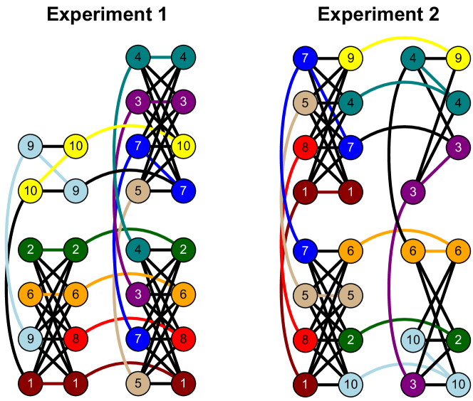
Similar embedding procedures to the one previously described were used for the larger experiments. For example, in Experiment 1, only 5 qubits define solutions of the computational problem. We needed 5 auxiliary qubits to transform the expression with 5-body interactions into an expression with only 2-body interactions. Embedding of this final expression required an additional of 18 qubits to satisfy the hardware connectivity requirements, for a total of 28 qubits. Table I in the SI material summarizes the number of qubits required in each step through to the final experimental realizations.

Even though the quantum device follows a quantum annealing protocol, the odds of measuring the ground state are not necessarily high. For example, in the 81 qubit experiment, only 13 out of 10,000 measurements yielded the desired solution. We attribute these low-percentages to the analog nature of the device and to precision limitations in the real values of the local fields and couplings among the qubits in the experimental setup. When compared to other problem implementations, physical problems such as lattice folding lack the structure of the Ramsey number problem Bian et al. (2012). In the lattice folding problem implemented here, the parameters defining the problem instances are arbitrary and do not fall into certain integral distinct values as in the case of the Ramsey number experiment, making precision issues more pronounced in our implementation.

To gain insights into the dynamics and evolution of the quantum system, we numerically simulated the superconducting array with a Bloch-Redfield model of the 8-qubit experiment (see SI material) which takes into account thermal fluctuations in the states due to the finite temperature (20mK) of the quantum device. For this 8-qubit experiment, the simulation predicted a ground state probability of 80.7 %, in excellent agreement with the experimentally observed value (80.3%). It is important to note that no adjustable parameters were used in our simulations to fit the data and all the parameters correspond to values measured directly from the quantum device. More details about the numerical simulations can be found in the SI.

As seen in Fig. 2(c), the temperature of the device is comparable with the minimum gap of the eight-qubit Hamiltonian. Therefore, we expect stronger excitation/relaxation near the gap closing, $\tau\approx 0.6$, due to exchange of energy with the environment, when compared to the other regimes of the annealing schedule where the gap is much larger than $k_{B}T$. In the absence of environment (a fully coherent process), our simulations indicate that that the success probability would be 100%, within numerical error. Fig. 2(d) shows that for the simulations at 20mK, the probability in the ground state goes down to $\sim 55\%$, but the same fluctuations make the system relax back to the ground state, yielding tan 80.27% success probability. This is due to the advantageous natural tendency of the system to approach a thermal equilibrium which favors the ground state after crossing the minimum energy gap. As previously discussed in similar numerical simulations of quantum annealing algorithms Amin, Truncik, and Averin (2009), strong coupling to the bath and non-Markovianity would require going beyond the Bloch-Redfield model Amin, Averin, and Nesteroff (2009), but the agreement between experimental and simulated results support the validity of the quantum mechanical model used to describe the device. Previously reported temperature dependence predictions for the tunneling rate on the same qubits Johnson et al. (2011) [3] and excellent agreement with the same level of theory used here reinforce the validity of our simulations for this 8-qubit instances.

We present the first quantum-mechanical implementation of lattice protein models using a programmable quantum device. We were able to encode and to solve the global minima solution for a small tetrapeptide and hexapeptide chain under several experimental schemes involving 5 and 8 qubits for the four-amino-acid sequence (Hydrophobic-Polar model) and 5, 27, 28, and 81 qubits experiments for the six amino-acid sequence under the Miyazawa-Jernigan model for general pairwise interactions. For the experiment with 8 qubits, we simulated the dynamics of the quantum device with a Redfield equation with no adjustable parameters, obtaining excellent agreement with experiment. Since the quantum annealing algorithm not only finds the ground state but also the low-lying excited states, it provides information about the relevant minimum energy compact structures of protein sequences Camacho and Thirumalai (1993) and it is useful to evaluate designability and stability such as that found in natural protein sequences, where the global minimum of free energy is well separated in energy from other misfolded states Anfinsen (1973). The approach employed here can be extended to treat other problems in biophysics and statistical mechanics such as molecular recognition, protein design, and sequence alignment Hartmann and Rieger (2004).

Supplementary Information

Summary

The paper Finding low-energy conformations of lattice protein models by quantum-annealing presents the first experimental and largest quantum annealing experiment related to an optimization problem in the physical sciences. In Sec. I, we summarize the construction of a more succinct version of the energy function describing the energy landscape of the six experimental realizations of the generalized lattice-folding model using Miyazawa-Jernigan pairwise interactions. In Sec. II, we present the necessary steps to transform the energy function into an expression which can be readily implemented in the quantum device. In Sec. III, we describe the quantum device used for our experiments and in Sec. IV we give details about the quantum simulations and results used to support the experimental outcomes.

I Transformation of the energy function of the lattice-folding model into the experimentally realizable spin-glass Hamiltonian

The energy function for the lattice model can be obtained as a sum of different contributions,

$$E_{p}(\bm{q})=E_{onsite}(\bm{q})+E_{pw}(\bm{q})+E_{ext}(\bm{q})$$ (S1)

where $E_{onsite}(\bm{q})$ penalizes configurations with overlaps among any two amino acids, $E_{pw}(\bm{q})$ accounts for nearest-neighbor pairwise-interaction energies among non-bonded amino acids, and $E_{ext}(\bm{q})$ refers to any external potentials other than the ones coming from interactions among the amino acids defining the protein. For amino acid sequences in vacuo, only $E_{onsite}$ and $E_{pw}$ are needed. The construction of these three-types of energy functions, in 2D and in 3D, for an arbitrary number of amino acids and interactions among them is explained in detail in Ref. 1. Hereforth, we will only focus on the case of energy functions in 2D.

I.1 Case of the six-amino acid sequence PSVKMA (Experiments 1-4)

For convenience, we reproduce Fig. 3 of the main text as Fig. S1, which illustrates and defines the six amino-acid sequence PSVKMA.

Figure S1: (a) Representation of the six-amino acid sequence, Proline-Serine-Valine-Lysine-Methionine-Alanine with its respective one-letter sequence notation, PSVKMA. We use the pairwise nearest-neighbor Miyazawa-Jernigan interaction energies reported in Table 3 of Ref. 2. (b) Divide and conquer approach showing three different schemes which independently solve the six-amino acid sequence PSVKMA on a two-dimensional lattice. We solved the problem under Scheme2 and 3 (Experiments 1 through 4). (c) Energy landscape for the valid conformations of the PSVKMA sequence. Results of the experimentally-measured probability outcomes are given as color-coded percentages according to each of the experimental realizations described in panel (b). Percentages for states with energy greater than zero are 32.70%, 59.88%, 8.00%, and 95.97% for Experiments 1 through 4, respectively.

As explained in the main text, the description of all possible 2D $N$-amino-acid fold in vacuo can be described by a bit string of length $2(N-1)$, with the first three bits held constant leaving $\ell=2N-5$ binary variables as the computational variables of the problem,

$$\bm{q}=\underbrace{01}_{turn1}\underbrace{0q_{1}}_{turn2}\underbrace{q_{2}q_{3}}_{turn3}\cdots\underbrace{q_{2N-6}q_{2N-5}}_{turn(N-1)}.$$ (S2)

For the case of $N=6$ (sequence PSVKMA), the problem is completely specified by the bit string

$$\bm{q}_{6AA}=\underbrace{01}_{turn1}\underbrace{0q_{1}}_{turn2}\underbrace{q_{2}q_{3}}_{turn3}\underbrace{q_{4}q_{5}}_{turn4}\underbrace{q_{6}q_{7}}_{turn5}.$$ (S3)

By using the construction in Ref. 1, the 7-bit energy function describing the sequence PSVKMA (Scheme 1 in Fig. S1) is given by,

$$\begin{split}E_{\textrm{\small{PSVKMA}}}&(\bm{q}_{6AA})=-q_{2}+8q_{1}q_{2}+15q_{2}q_{3}-18q_{1}q_{2}q_{3}-3q_{1}q_{4}+12q_{1}q_{2}q_{4}+4q_{3}q_{4}+3q_{1}q_{3}q_{4}\\ &-6q_{2}q_{3}q_{4}-12q_{1}q_{2}q_{3}q_{4}+4q_{2}q_{5}+3q_{1}q_{2}q_{5}-15q_{2}q_{3}q_{5}+15q_{4}q_{5}+3q_{1}q_{4}q_{5}\\ &-6q_{2}q_{4}q_{5}-12q_{1}q_{2}q_{4}q_{5}-15q_{3}q_{4}q_{5}+28q_{2}q_{3}q_{4}q_{5}-2q_{1}q_{2}q_{6}-4q_{3}q_{6}+2q_{2}q_{3}q_{6}\\ &+13q_{1}q_{2}q_{3}q_{6}-2q_{1}q_{4}q_{6}+4q_{1}q_{2}q_{4}q_{6}+2q_{3}q_{4}q_{6}+13q_{1}q_{3}q_{4}q_{6}+4q_{2}q_{3}q_{4}q_{6}\\ &-37q_{1}q_{2}q_{3}q_{4}q_{6}+7q_{5}q_{6}+2q_{2}q_{5}q_{6}+13q_{1}q_{2}q_{5}q_{6}+4q_{3}q_{5}q_{6}+9q_{2}q_{3}q_{5}q_{6}\\ &-33q_{1}q_{2}q_{3}q_{5}q_{6}-20q_{4}q_{5}q_{6}+13q_{1}q_{4}q_{5}q_{6}+4q_{2}q_{4}q_{5}q_{6}-37q_{1}q_{2}q_{4}q_{5}q_{6}+9q_{3}q_{4}q_{5}q_{6}\\ &-33q_{1}q_{3}q_{4}q_{5}q_{6}-37q_{2}q_{3}q_{4}q_{5}q_{6}+99q_{1}q_{2}q_{3}q_{4}q_{5}q_{6}-4q_{2}q_{7}+4q_{2}q_{3}q_{7}+7q_{4}q_{7}\\ &+2q_{2}q_{4}q_{7}+13q_{1}q_{2}q_{4}q_{7}+4q_{3}q_{4}q_{7}+9q_{2}q_{3}q_{4}q_{7}-33q_{1}q_{2}q_{3}q_{4}q_{7}+4q_{2}q_{5}q_{7}\\ &-18q_{4}q_{5}q_{7}+9q_{2}q_{4}q_{5}q_{7}-33q_{1}q_{2}q_{4}q_{5}q_{7}-33q_{2}q_{3}q_{4}q_{5}q_{7}+62q_{1}q_{2}q_{3}q_{4}q_{5}q_{7}+7q_{6}q_{7}\\ &+2q_{2}q_{6}q_{7}+13q_{1}q_{2}q_{6}q_{7}+4q_{3}q_{6}q_{7}+9q_{2}q_{3}q_{6}q_{7}-33q_{1}q_{2}q_{3}q_{6}q_{7}-20q_{4}q_{6}q_{7}\\ &+13q_{1}q_{4}q_{6}q_{7}+4q_{2}q_{4}q_{6}q_{7}-37q_{1}q_{2}q_{4}q_{6}q_{7}+9q_{3}q_{4}q_{6}q_{7}-33q_{1}q_{3}q_{4}q_{6}q_{7}-37q_{2}q_{3}q_{4}q_{6}q_{7}\\ &+99q_{1}q_{2}q_{3}q_{4}q_{6}q_{7}-18q_{5}q_{6}q_{7}+9q_{2}q_{5}q_{6}q_{7}-33q_{1}q_{2}q_{5}q_{6}q_{7}-33q_{2}q_{3}q_{5}q_{6}q_{7}\\ &+62q_{1}q_{2}q_{3}q_{5}q_{6}q_{7}+53q_{4}q_{5}q_{6}q_{7}-33q_{1}q_{4}q_{5}q_{7}q_{7}-37q_{2}q_{4}q_{6}q_{6}q_{7}+99q_{5}q_{2}q_{4}q_{5}q_{6}q_{7}\\ &-33q_{3}q_{1}q_{5}q_{6}q_{7}+62q_{1}q_{4}q_{4}q_{5}q_{6}q_{7}+99q_{2}q_{3}q_{4}q_{5}q_{6}q_{7}-190q_{1}q_{2}q_{3}q_{4}q_{5}q_{6}q_{7}.\end{split}$$ (S4)

As shown in Fig. S1, expressions for each of the different experiments in Schemes 2 and 3 can be sequentially obtained by fixing the value of some of the variables in $E_{\textrm{\small{PSVKMA}}}(\bm{q}_{6AA})$.

The energy function for Experiment 1 is obtained by evaluating $E_{\textrm{\small{PSVKMA}}}(\bm{q}_{6AA})$ with $q_{1}=1$ (third amino-acid moves to the right) and $q_{2}=0$ (fourth amino-acid moves either down or right, exploiting upper/lower half-plane symmetry). After relabeling the five remaining variables so that their labels go from 1-5 instead of 3-7, i.e., $\bm{q}_{6AA}=010q_{1}q_{2}q_{3}q_{4}q_{5}q_{6}q_{7}\xrightarrow[\rm{relabel}]{q_{1}=1,q_{2}=0}\bm{q}_{exp1}=01010q_{1}q_{2}q_{3}q_{4}q_{5}$, the resulting expression describing the energy landscape for Experiment 1 is given by

$$\begin{split}E^{exp1}_{\textrm{\small{PSVKMA}}}&(\bm{q}_{exp1})=-3q_{2}+7q_{1}q_{2}+18q_{2}q_{3}-15q_{1}q_{2}q_{3}-4q_{1}q_{4}-2q_{2}q_{4}+15q_{1}q_{2}q_{4}\\ &+7q_{3}q_{4}+4q_{1}q_{3}q_{4}-7q_{2}q_{3}q_{4}-24q_{1}q_{2}q_{3}q_{4}+7q_{2}q_{5}+4q_{1}q_{2}q_{5}-18q_{2}q_{3}q_{5}\\ &+7q_{4}q_{5}+4q_{1}q_{4}q_{5}-7q_{2}q_{4}q_{5}-24q_{1}q_{2}q_{4}q_{5}-18q_{3}q_{4}q_{5}+20q_{2}q_{3}q_{4}q_{5}\\ &+29q_{1}q_{2}q_{3}q_{4}q_{5}\end{split}$$ (S5)

The energy function for Experiment 4 is obtained by evaluating $E_{\textrm{\small{PSVKMA}}}(\bm{q}_{6AA})$ with $q_{1}=0$ (third amino-acid moves down). After renaming the six remaining variables so that their labels span 1-6 instead of 2-7, i.e., $\bm{q}_{6AA}=010q_{1}q_{2}q_{3}q_{4}q_{5}q_{6}q_{7}\xrightarrow[\rm{relabel}]{q_{1}=0}\bm{q}_{exp4}=0100q_{1}q_{2}q_{3}q_{4}q_{5}q_{6}$, the resulting expression describing the energy landscape for Experiment 4 is given by

$$\begin{split}E^{exp4}_{\textrm{\small{PSVKMA}}}&(\bm{q}_{exp4})=-q_{1}+15q_{1}q_{2}+4q_{2}q_{3}-6q_{1}q_{2}q_{3}+4q_{1}q_{4}-15q_{1}q_{2}q_{4}+15q_{3}q_{4}-6q_{1}q_{3}q_{4}\\ &-15q_{2}q_{3}q_{4}+28q_{1}q_{2}q_{3}q_{4}-4q_{2}q_{5}+2q_{1}q_{2}q_{5}+2q_{2}q_{3}q_{5}+4q_{1}q_{2}q_{3}q_{5}+7q_{4}q_{5}\\ &+7q_{5}q_{6}+2q_{1}q_{4}q_{5}+4q_{2}q_{4}q_{5}+9q_{1}q_{2}q_{4}q_{5}-20q_{3}q_{4}q_{5}+4q_{1}q_{3}q_{4}q_{5}+9q_{2}q_{3}q_{4}q_{5}\\ &-37q_{1}q_{2}q_{3}q_{4}q_{5}-4q_{1}q_{6}+4q_{1}q_{2}q_{6}+7q_{3}q_{6}+2q_{1}q_{3}q_{6}+4q_{2}q_{3}q_{6}+9q_{1}q_{2}q_{3}q_{6}\\ &+4q_{1}q_{4}q_{6}-18q_{3}q_{4}q_{6}+9q_{1}q_{3}q_{4}q_{6}-33q_{1}q_{2}q_{3}q_{4}q_{6}+2q_{1}q_{5}q_{6}+4q_{2}q_{5}q_{6}-20q_{3}q_{5}q_{6}\\ &+9q_{1}q_{2}q_{5}q_{6}+4q_{1}q_{3}q_{5}q_{6}+9q_{2}q_{3}q_{5}q_{6}-37q_{1}q_{2}q_{3}q_{5}q_{6}-18q_{4}q_{5}q_{6}+9q_{1}q_{4}q_{5}q_{6}\\ &-33q_{1}q_{2}q_{4}q_{5}q_{6}+53q_{3}q_{4}q_{5}q_{6}-37q_{1}q_{3}q_{4}q_{5}q_{6}-33q_{2}q_{3}q_{4}q_{5}q_{6}+99q_{1}q_{2}q_{3}q_{4}q_{5}q_{6}\end{split}$$ (S6)

The energy function for Experiment 2 is obtained by evaluating $E^{exp4}_{\textrm{\small{PSVKMA}}}(\bm{q}_{exp4})$ with $q_{1}=0$ (fourth amino-acid moves either down or right). After renaming the five remaining variables so that their labels span 1-5 instead of 2-6, i.e., $\bm{q}_{exp4}=0100q_{1}q_{2}q_{3}q_{4}q_{5}q_{6}\xrightarrow[\rm{relabel}]{q_{1}=0}\bm{q}_{exp2}=01000q_{1}q_{2}q_{3}q_{4}q_{5}$, the resulting expression describing the energy landscape for Experiment 2 is given by

$$\begin{split}E^{exp2}_{\textrm{\small{PSVKMA}}}&(\bm{q}_{exp2})=4q_{1}q_{2}+15q_{2}q_{3}-15q_{1}q_{2}q_{3}-4q_{1}q_{4}+2q_{1}q_{2}q_{4}+7q_{3}q_{4}+4q_{1}q_{3}q_{4}\\ &-20q_{2}q_{3}q_{4}+9q_{1}q_{2}q_{3}q_{4}+7q_{2}q_{5}+4q_{1}q_{2}q_{5}-18q_{2}q_{3}q_{5}+7q_{4}q_{5}+4q_{1}q_{4}q_{5}\\ &-20q_{2}q_{4}q_{5}+9q_{1}q_{2}q_{4}q_{5}-18q_{3}q_{4}q_{5}+53q_{2}q_{3}q_{4}q_{5}-33q_{1}q_{2}q_{3}q_{4}q_{5}.\end{split}$$ (S7)

Finally, the energy function for Experiment 3 is obtained by evaluating $E^{exp4}_{\textrm{\small{PSVKMA}}}(\bm{q}_{exp4})$ with $q_{1}=1$, $q_{2}=0$(fourth amino-acid moves left) and $q_{4}=0$ (fifth amino-acid moves either down or left), exploiting the constrains imposed by the three fixed amino-acids (P,S, and V). After renaming the three remaining variables so that their labels are $q_{1},q_{2}$ and $q_{3}$ instead of $q_{3},q_{5}$, and $q_{7}$, i.e., $\bm{q}_{exp4}=0100q_{1}q_{2}q_{3}q_{4}q_{5}q_{6}\xrightarrow[\rm{relabel}]{q_{1}=1,q_{2}=0,q_{4}=0}\bm{q}_{exp3}=010010q_{1}0q_{2}q_{3}$, the resulting expression describing the energy landscape for Experiment 3 is given by

$$E^{exp3}_{\textrm{\small{PSVKMA}}}(\bm{q}_{exp3})=-1-4q_{3}+9q_{1}q_{3}+9q_{2}q_{3}-16q_{1}q_{2}q_{3}$$ (S8)

I.2 Case of the four-amino acid sequence HPPH (Experiment 5)

Besides the six-amino acid sequence considered above, we also constructed the energy function for the simplest of all sequences within lattice protein models, the HPPH four-amino acid sequence within the HP model. For $N=4$, we can specify any of its folds by the bit string $\bm{q}_{exp5}=010q_{1}q_{2}q_{3}$. The three-bit energy function describing the energy landscape of Experiment 5 (see Fig. S2) is given by,

$$E_{HPPH}(\bm{q}_{exp5})=-q_{2}+2q_{1}q_{2}+2q_{2}q_{3}-3q_{1}q_{2}q_{3}$$ (S9)

I.3 Case of the four-amino acid sequence HPPH under external constraints (Experiment 6)

A more realistic in vivo picture involves the presence of chaperone proteins assisting the folding dynamics towards the global minima. Chaperones, molecular docking, and molecular recognition are examples of problems which can be studied by adding external potentials, $E_{ext}(\bm{q})$, beyond the intrinsic interactions defined by the amino-acid chain, $E_{onsite}(\bm{q})$ and $E_{pw}(\bm{q})$ (see Eq. S1). The first consequence of adding an external potential $E_{ext}(\bm{q})$ (as the chaperone-like environment surrounding the small four-amino-acid sequence HPPH, illustrated in Fig. S2 by the pink-shaded area near the peptide) is that we can no longer exploit the symmetry of the solution space for upper and lower half plane conformations. Therefore, we cannot set the first variable of the turn associated with the third amino-acid to zero. Under external potentials, we specify arbitrary folds of the four-amino acid problem by $\bm{q}_{exp6}=01q_{1}q_{2}q_{3}q_{4}$, where $q_{1}q_{2}(q_{3}q_{4})$ encodes the orientation of the second (third) bond.

Figure S2: Energy landscape for the four amino-acid sequence HPPH, (a) in vacuo (Experiment 5), and (b) under the presence of a chaperone-like environment (Experiment 6) represented by the red-shaded region. In panel (a) [panel (b)], percentages indicate the experimentally measured probabilities of each state collected over 10,000 [28,672] runs of the quantum annealing algorithm described in Sec. III.3. In the case of Experiment 6, numerical results from the Bloch-Redfield model discussed in Sec IV are included in parenthesis. Although the variables involved in Experiment 5 (Experiment 6) are described by $\bm{q}_{exp5}=010q_{1}q_{2}q_{3}|q_{4}q_{4^{\prime}}$ ($\bm{q}_{exp6}=01q_{1}q_{2}q_{3}q_{4}|q_{5}q_{6}q_{2^{\prime}}q_{4^{\prime}}$), under each fold we write only the physically-relevant variables which define the conformation. Since we show some experimental outcomes also for states with $E>0$, then it is natural to find states which violate either the and condition or the ferromagnetic condition; for these cases we explicitly write the auxilliary variables which went into the quantum hardware. For example, in Experiment 5 [panel (a)], the state $\bm{q}_{exp5}=010101|11$ violates the and condition since $q_{4}\neq q_{2}q_{3}$. In the case of the state $\bm{q}_{exp5}=010010|01$ the ferromagnetic condition for $q_{4}$ is violated since $q_{4}\neq q_{4^{\prime}}$. Each overlap of the amino acids with the chaperone raises energy by four units, whereas overlaps (red crossings) among amino acids in the chain raise energy by two units.

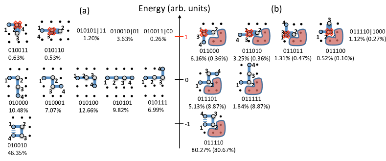
The external potential penalizes conformations in which either the third or fourth amino acid go into the chaperone region is:

$$\begin{split}E_{chap}(\bm{q}_{exp6})&=\lambda^{d}_{ext}(1-q_{1})(1-q_{2})+\lambda^{r}_{ext}(1-q_{1})q_{2}+\lambda^{dr}_{ext}(1-q_{1})(1-q_{2})(1-q_{3})q_{4}\\ &+\lambda^{rd}_{ext}(1-q_{1})q_{2}(1-q_{3})(1-q_{4})\end{split}$$ (S10)

The penalty $\lambda^{d}_{ext}$ raises energy only when the third amino-acid moves down ($q_{1}=0,q_{2}=0$), $\lambda^{r}_{ext}$ raises energy only when the third amino-acid moves right ($q_{1}=0,q_{2}=1$), $\lambda^{dr}_{ext}$ raises energy only when the third amino-acid moves down and the fourth-amino acid moves right ($q_{1}=0,q_{2}=0,q_{3}=0,q_{4}=1$), and the last penalty, $\lambda^{rd}_{ext}$, raises energy only when the third amino-acid moves down and the fourth-amino acid moves right ($q_{1}=0,q_{2}=1,q_{3}=0,q_{4}=0$). Each overlap of the amino acids with the chaperone increases energy by four units, i.e., $\lambda^{d}_{ext}=\lambda^{r}_{ext}=\lambda^{dr}_{ext}=\lambda^{rd}_{ext}=4$.

When the third amino acid is also allowed to move upwards, the energy function for the HPPH chain in vacuo is given by,

$$\begin{split}E_{HPPH}(\bm{q}_{exp6})&=q_{1}-q_{3}+q_{1}q_{3}+2q_{2}q_{3}-4q_{1}q_{2}q_{3}+2q_{1}q_{4}\\ &-3q_{1}q_{2}q_{4}+2q_{3}q_{4}-4q_{1}q_{3}q_{4}-3q_{2}q_{3}q_{4}+7q_{1}q_{2}q_{3}q_{4}\end{split}$$ (S11)

After adding Eq. S10 and Eq. S11, the resulting energy function for the HPPH peptide in the presence of the “chaperone” environment illustrated in Fig. S2, is given by,

$$\begin{split}E_{HPPH,chap}(\bm{q}_{exp6})&=4-3q_{1}+4q_{2}-4q_{1}q_{2}-q_{3}+q_{1}q_{3}-2q_{2}q_{3}+4q_{4}-2q_{1}q_{4}\\ &-8q_{2}q_{4}+5q_{1}q_{2}q_{4}-2q_{3}q_{4}+5q_{2}q_{3}q_{4}-q_{1}q_{2}q_{3}q_{4},\end{split}$$ (S12)

II Embbedding of problem instances into the quantum hardware

II.1 Reduction of high-order terms to a 2-body Ising-like Hamiltonian

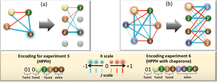
As explained in the main text, although the above energy expressions (Eqs. S4S, S5S, S6S, S7S, S8S, S9S, and S12S) describe the desired energy landscape, they are not suitable for experimental implementation. We need to reduce the degree of the high-order terms (cubic, cuartic, etc) to a quadratic expression (up to 2-body interactions). These high-order terms indicate many-body interactions which are not experimentally feasible within the current quantum device. To achieve this without altering the low-energy spectra ($E\leq 0$) where the target minima is supposed to be found, we use the technique described in Ref. Perdomo2008, 1. In the main text, we presented the simplest case where only one reduction was required (expression for Experiment 3, Eq. S8). In the following we will focus on the next most complex case (Experiment 6, Eq. S12) which can be easily generalized to obtain any of the 2-body energy expressions for the larger experiments.

We introduce two ancilla binary variables, $q_{5}$ and $q_{6}$, and substitute Eq. S12 with products of the form $q_{1}q_{2}$ into $q_{5}$ and $q_{3}q_{4}$ into $q_{6}$. This substitution transforms the energy expression (Eq. S12) into a quadratic expression, e.g, the highest-order term which is quadratic, $q_{1}q_{2}q_{3}q_{4}$, is replaced by $q_{5}q_{6}$ which becomes quadratic, as desired. Under these substitutions, whenever we have six-variable assignments, $\bm{q}_{exp6}=01q_{1}q_{2}q_{3}q_{4}|q_{5}q_{6}$, such that $q_{6}=q_{1}\wedge q_{2}=q_{1}q_{2}$ and $q_{6}=q_{3}\wedge q_{4}=q_{3}q_{4}$, we have the same energy spectrum as the one for the original quartic, four-variable expression. Since these two ancilla are new variables whose values are independent of the four original variables, we need to penalize six-variable assignments whenever $q_{5}\neq q_{1}q_{2}$ and $q_{6}\neq q_{3}q_{4}$. For every “collapse” of the form $q_{i}q_{j}\rightarrow r_{k}$, we add the penalty $E_{\wedge}(q_{i},q_{j},r_{k};\delta_{ij})=\delta_{ij}(3r_{k}+q_{i}q_{j}-2q_{i}r_{k}-2q_{j}\delta_{ij})$, where $\delta_{ij}$ is a positive number representing a penalty chosen (for more details see Ref. 1) such that assignments violating this and condition correspond to free-energies $E>0$, outside the relevant search region ($E\leq 0$). The function $E_{\wedge}(q_{i},q_{j},r_{k};\delta_{ij})=0$ only if $r_{k}=q_{i}q_{j}$ and $E_{\wedge}(q_{i},q_{j},r_{k};\delta_{ij})>0$ if $r_{k}\neq q_{i}q_{j}$. The six-variable expression resulting from the insertion of the new ancilla variables plus the penalty function becomes,

$$\begin{split}E_{HPPH,chap}^{2body}(\bm{q})&=E_{HPPH,chap}(q_{1},q_{2},q_{3},q_{4};q_{1}q_{2}\rightarrow q_{5},q_{3}q_{4}\rightarrow q_{6})\\ &+E_{\wedge}(q_{1},q_{2},q_{5};\delta_{12})+E_{\wedge}(q_{3},q_{4},q_{6};\delta_{34})\\ &=4-3q_{1}+4q_{2}+6q_{1}q_{2}-q_{3}+q_{1}q_{3}-2q_{2}q_{3}+4q_{4}-2q_{1}q_{4}-8q_{2}q_{4}+4q_{3}q_{4}\\ &+14q_{5}-12q_{1}q_{5}-12q_{2}q_{5}+5q_{4}q_{5}+10q_{6}+5q_{2}q_{6}-8q_{3}q_{6}-8q_{4}q_{6}-q_{5}q_{6}\end{split}$$ (S13)

where according to the criteria in Ref. 1, we have chosen $\delta_{12}=6$, and $\delta_{34}=4$.

To rewrite this quadratic form in terms of the spin variables $\{s_{i}\}$, we apply the transformation $q_{i}\equiv\frac{1}{2}(1-s_{i})$ to each of the binary variables,

$$\begin{split}E_{HPPH,chap}^{Ising}&=10+\frac{13}{4}s_{1}+\frac{3}{4}s_{2}+\frac{7}{4}s_{3}+\frac{1}{4}s_{4}-2s_{5}-2s_{6}+\frac{3}{2}s_{1}s_{2}+\frac{1}{4}s_{1}s_{3}-\frac{1}{2}s_{2}s_{3}\\ &-\frac{1}{2}s_{1}s_{4}-2s_{2}s_{4}+s_{3}s_{4}-3s_{1}s_{5}-3s_{2}s_{5}+\frac{5}{4}s_{4}s_{5}+\frac{5}{4}s_{2}s_{6}-2s_{3}s_{6}\\ &-2s_{4}s_{6}-\frac{1}{4}s_{5}s_{6}\end{split}$$ (S14)

After substracting the constant (independent term), we can fulfill the requirement that $\lvert h_{i}\rvert\leq 1$ and $\lvert J_{ij}\rvert\leq 1$ by scaling all coefficients of Eq. S14 down by the maximum absolute value of all coefficients. The renormalized quadratic expression is given by,

$$\begin{split}E_{exp6}^{unembedded}(\bm{s})&=\frac{4}{13}(E_{HPPH,chap}^{ising}-10)\\ &=(13s_{1}+3s_{2}+7s_{3}+s_{4}-8s_{5}-8s_{6}+6s_{1}s_{2}+s_{1}s_{3}-2s_{2}s_{3}\\ &-2s_{1}s_{4}-8s_{2}s_{4}+4s_{3}s_{4}-12s_{1}s_{5}-12s_{2}s_{5}+5s_{4}s_{5}+5s_{2}s_{6}-8s_{3}s_{6}\\ &-8s_{4}s_{6}-s_{5}s_{6})/13\end{split}$$ (S15)

The final Ising spin-glass Hamiltonian (before embedding into the quantum device) can be obtained by the substitution $s_{i}\rightarrow\sigma^{z}_{i}$.

$$\begin{split}H^{\text{unembedded}}_{exp6}&=(13\sigma^{z}_{1}+3\sigma^{z}_{2}+7\sigma^{z}_{3}+\sigma^{z}_{4}-8\sigma^{z}_{5}-8\sigma^{z}_{6}+6\sigma^{z}_{1}\sigma^{z}_{2}+\sigma^{z}_{1}\sigma^{z}_{3}-2\sigma^{z}_{2}\sigma^{z}_{3}\\ &-2\sigma^{z}_{1}\sigma^{z}_{4}-8\sigma^{z}_{2}\sigma^{z}_{4}+4\sigma^{z}_{3}\sigma^{z}_{4}-12\sigma^{z}_{1}\sigma^{z}_{5}-12\sigma^{z}_{2}\sigma^{z}_{5}+5\sigma^{z}_{4}\sigma^{z}_{5}+5\sigma^{z}_{2}\sigma^{z}_{6}-8\sigma^{z}_{3}\sigma^{z}_{6}\\ &-8\sigma^{z}_{4}\sigma^{z}_{6}-\sigma^{z}_{5}\sigma^{z}_{6})/13\end{split}$$ (S16)

II.2 Embedding into the quantum hardware

Eq. S16 does not fulfill the chip-connectivity requirements (see Fig. S3) for the primal graph representing Eq. S16. This limitation is fixed at the cost of adding two new qubits serving as replicas of the two qubits which are linked by more than four connections. To enforce that the replicas of the $i$-th qubit ($\sigma^{z}_{i^{\prime}}$) produce the same outcome as the original $i$-th qubit, we couple $\sigma^{z}_{i}$ and $\sigma^{z}_{i^{\prime}}$ with a strong ferromagnetic coupling, such that whenever the outcomes of the two variables are different they get penalized by a chosen penalty factor $\gamma_{i}>0$. The function which performs this penalization for each replica $i$-th qubit is $H_{FM}(\{\sigma^{z}_{i}\};\gamma_{i})=\gamma_{i}(1-\sigma^{z}_{i}\sigma^{z}_{i^{\prime}})$. Notice that $H_{FM}(\{\sigma^{z}_{i}\};\gamma_{i})=0$, if $s_{i}=s_{i^{\prime}}=\pm 1$, but $H_{FM}(\{\sigma^{z}_{i}\};\gamma_{i})=2\gamma_{i}$, if $s_{i}\neq s_{i^{\prime}}$. For this study, a value of $\gamma_{2}=\gamma_{4}=1$ suffices to leave assignments which violate this condition outside the region of interest with $E\leq 0$.

The redistribution of the connections among the original and primed qubits is given in the right panel of Fig. S3. The modified function taking into account the added ferromagnetic couplings is,

$$\begin{split}\tilde{H}_{exp6}&=H^{\text{unembedded}}_{exp6}(\sigma^{z}_{2}\rightarrow\{\sigma^{z}_{2},\sigma^{z}_{2^{\prime}}\};\sigma^{z}_{4}\rightarrow\{\sigma^{z}_{4},\sigma^{z}_{4^{\prime}}\})\\ &+H_{FM}(\{\sigma^{z}_{2}\};\gamma_{2}=1)+H_{FM}(\{\sigma^{z}_{4}\};\gamma_{4}=1)\\ &=(13\sigma^{z}_{1}+3\sigma^{z}_{2}+7\sigma^{z}_{3}+\sigma^{z}_{4}-8\sigma^{z}_{5}-8\sigma^{z}_{6}+6\sigma^{z}_{1}\sigma^{z}_{2^{\prime}}+\sigma^{z}_{1}\sigma^{z}_{3}-2\sigma^{z}_{2}\sigma^{z}_{3}\\ &-2\sigma^{z}_{1}\sigma^{z}_{4^{\prime}}-8\sigma^{z}_{2^{\prime}}\sigma^{z}_{4}+4\sigma^{z}_{3}\sigma^{z}_{4}-12\sigma^{z}_{1}\sigma^{z}_{5}-12\sigma^{z}_{2}\sigma^{z}_{5}+5\sigma^{z}_{4}\sigma^{z}_{5}+5\sigma^{z}_{2^{\prime}}\sigma^{z}_{6}-8\sigma^{z}_{3}\sigma^{z}_{6}\\ &-8\sigma^{z}_{4^{\prime}}\sigma^{z}_{6}-\sigma^{z}_{5}\sigma^{z}_{6})/13+(1-\sigma^{z}_{2}\sigma^{z}_{2^{\prime}})+(1-\sigma^{z}_{4}\sigma^{z}_{4^{\prime}})\end{split}$$ (S17)

Again, we subtract the independent constant terms from the insertion of the $H_{FM}$ functions. The final expression, which is implementable in the quantum device is,

$$\begin{split}H_{exp6}&=\tilde{H}_{exp6}-2=(13\sigma^{z}_{1}+3\sigma^{z}_{2}+7\sigma^{z}_{3}+\sigma^{z}_{4}-8\sigma^{z}_{5}-8\sigma^{z}_{6}+6\sigma^{z}_{1}\sigma^{z}_{2^{\prime}}+\sigma^{z}_{1}\sigma^{z}_{3}-2\sigma^{z}_{2}\sigma^{z}_{3}\\ &-2\sigma^{z}_{1}\sigma^{z}_{4^{\prime}}-8\sigma^{z}_{2^{\prime}}\sigma^{z}_{4}+4\sigma^{z}_{3}\sigma^{z}_{4}-12\sigma^{z}_{1}\sigma^{z}_{5}-12\sigma^{z}_{2}\sigma^{z}_{5}+5\sigma^{z}_{4}\sigma^{z}_{5}+5\sigma^{z}_{2^{\prime}}\sigma^{z}_{6}-8\sigma^{z}_{3}\sigma^{z}_{6}\\ &-8\sigma^{z}_{4^{\prime}}\sigma^{z}_{6}-\sigma^{z}_{5}\sigma^{z}_{6}-13\sigma^{z}_{2}\sigma^{z}_{2^{\prime}}-13\sigma^{z}_{4}\sigma^{z}_{4^{\prime}})/13\end{split}$$ (S18)

Figure S3: In the graphs presented in (a) and (b), each node denotes a qubit, and the color and extent of its glow denotes the sign and strength of its corresponding longitudinal field, $h_{i}$. The edges represent the interaction couplings, $J_{ij}$, where color indicates sign and thickness indicates magnitude. The maximum couplings are indicated in the figure by heavy lines. (a) Primal graph (left) and the embedded representation of the expression implemented in the quantum hardware for Experiment 5 (HPPH in vacuo). (b) Primal graph (left) and the embedded eight-qubit expression (Eq. S18) for Experiment 6 (HPPH in the chaperone-lke environment).

Table 1: Number of qubits needed for each one of the six experiments described in Fig. S1 and Fig. S2. The most compact version of the energy function corresponds to the second column. Each one of the steps, reduction of high-order terms in the energy function towards a 2-body Ising-like Hamiltonian and embedding of this Ising expression to fulfill the physical connectivity of the qubits in the device, requires more auxiliary qubits. The final column reports the number of qubits in the experimentally implemented expression of the energy function.

	Number of qubits needed
Experiment #	energy function	Ising Hamiltonian	hardware-embedded expression
1	5	10	28
2	5	10	27
3	3	4	5
4	6	19	81
5	3	4	5
6	4	6	8

The embeddings for Experiments 3 and 4 are shown in Fig. 4 and Fig. 1 of the main text, respectively. The embeddings corresponding to Experiment 5 and 6 are represented in Fig. S3, while the embedding for the medium size problem instances (Experiments 1 and 2) are represented in Fig. S4.

Figure S4: Embedding of Experiments 1 and 2 into the quantum hardware. The 28 qubits (27 qubits) from Experiment 1 (Experiment 2) have been relabeled to show the qubits which were strongly ferromagnetically coupled representing the same variable and biased to have the same experimental outcomes. Both problem instances resulted in ten-qubit spin-glass Hamiltonians after reducing their energy expressions to the Ising-like 2-body interaction expression. The additional qubits are part of the embedding procedure used to fulfill the arbitrary connectivity of the Ising expression, allowing for couplings of qubits that are not directly coupled in hardware.

III Experimental details

III.1 The processor chip

All experiments discussed herein were conducted on a sample fabricated in a four Nb layer superconducting integrated circuit process employing a standard Nb/AlOx/Nb trilayer, a TiPt resistor layer, and planarized SiO₂ dielectric layers deposited with a plasma-enhanced chemical vapour deposition process. Design rules included 0.25 $\mu m$ lines and spaces for wiring layers and a minimum junction diameter of 0.6 $\mu m$. Experiments were conducted in an Oxford Instruments Triton 400 Cryofree DR at a temperature of 20 mK.

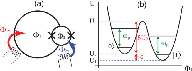
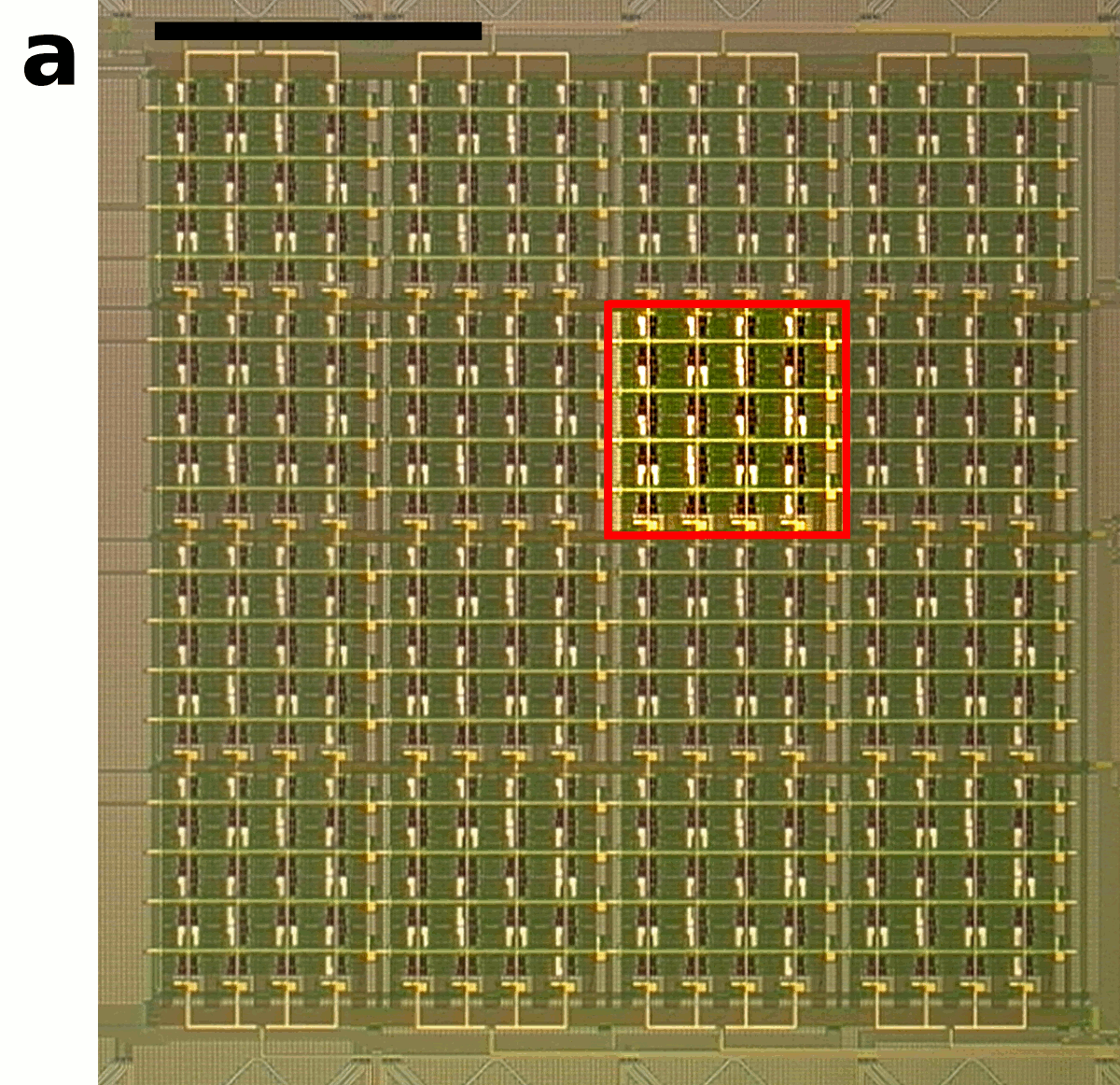
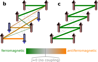
The sample processor chip contains a coupled array of 128 qubits of a design discussed in Ref. 3. Each qubit is an rf-SQUID flux qubit with a double-well potential, as depicted in Fig. S5. They are magnetically coupled with sign and magnitude tunable couplers in a manner described in Ref. 4. The array is built up of 16 eight-qubit unit cells. For example, Experiment 6 was conducted using a single unit cell (highlighted in Fig. S6a). The connectivity of qubits within the unit cell is shown schematically in Fig. S6b.

Three different chips available with this same architecture were used to run the different problem instances (Experiments 1-6, Fig. S1 and S2). Experiments 1, 2, and 4 were run in one chip, while Experiment 3 and 5 used a different chip. Experiment 6 used the same chip and unit cell used in Ref. 5. Since all the chips have the same architecture and design but different calibration parameters, we will focus on the chip used to run Experiment 6, and report all the parameters used to run the numerical simulation reported in Sec. IV.

Figure S5: (a) Illustration of a single rf-SQUID flux qubit. $\Phi_{1x}$ is the flux bias applied to the major (qubit) loop, and $\Phi_{2x}$ is the flux bias applied to the minor (CJJ) loop. (b) Cross-section of the double-well potential of an rf-SQUID flux qubit, with 4 localized energy levels marked. $\Phi_{1x}$ primarily affects the qubit bias $\epsilon$, whereas $\Phi_{2x}$ affects both the barrier height $\delta U_{0}$ and $\epsilon$.

III.2 Magnetic Environment

The magnetic field in the sample space was controlled with three concentric high permeability shields and an innermost superconducting shield. Further active compensation of residual fields was achieved with compensation coils oriented along three axes, and used in conjunction with on-chip superconducting quantum interference device (SQUID) magnetometers located near each of the four corners of the processor block (Fig. S6a). Compensation coils were adjusted to minimise the magnetic field measured at the magnetometers while the chip was at 4.2 K. The chip was then thermally cycled just above and then back down through its superconducting transition temperature at this minimal field. We estimate that the chip was cooled through its superconducting transition with a field normal to the chip surface $|B_{\perp}|<2.5~{}\mathrm{nT}$, and that parallel to its surface $|B_{\parallel}|<3.6~{}\mathrm{nT}$ over the area of active circuitry.

Figure S6: (a) Optical photograph of a portion of a partially fabricated 128 qubit chip. The block of eight qubits used in this experiment is outlined in red. (b) Artificial spins are connected in a complete bipartite graph $K_{4,4}$, and interact via couplers which are continuously tunable from ferromagnetic to antiferromagnetic interaction. A line between artificial spins indicates that a coupler is present. The colouring indicates one possible arrangement of coupler settings. (c) An example of how a linear ferromagnetic Ising spin chain could be implemented by selectively tuning some couplers to a ferromagnetic setting $(J<0)$ (green), and turning off the rest $(J=0)$.

III.3 Experimental method

The experiment discussed in the manuscript is outlined in Table 2.

Table 2: Outline of experiment

1. Initialisation

   1. Calibration: measure intrinsic device parameters such as junction $I_{c}$, qubit inductance, transformer mutual inductances, etc.

   2. Homogenisation: use on-chip programmable flux biases to ensure $I_{p}$ of the different qubits match during annealing.

2. Annealing & read-out

   1. Set h, J

   2. Anneal (reduce $A(\tau)$ and increase $B(\tau)$)

   3. Read state of spins

The steps in part I were performed once and would, in general, only be performed once for a new chip. The calibration step I-1 is performed by measuring the circulating current $I_{p}$ in each qubit, and its dependence on the CJJ loop flux bias $\Phi_{2x}$. From this information, one can extract the qubit critical current $I_{c}$ and inductance $L$. Details of this procedure are discussed in detail in section IV.A of Ref. 3. Given these qubit parameters, the effective inter-qubit coupling strength attained by the tunable couplers can be determined. This was done by measuring the difference in magnetic flux coupled into a qubit B between states $|\uparrow\rangle$ and $|\downarrow\rangle$ of a qubit A. This coupled flux was measured as a function of the setting of the tunable coupler between qubits A and B, in a manner described in detail in Ref. 6.

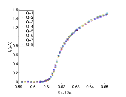
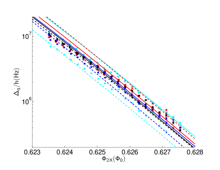
Once the device parameters for each qubit have been extracted, the effective junction $I_{c}$ and inductance $L$ of each qubit are tuned with on-chip tuning structures so as to make them as similar to each other as possible. The goal of this homogenisation procedure is to ensure that the circulating currents, $I_{p}$, of several qubits remain close to each other in magnitude while the qubits undergo annealing. This procedure is discussed in detail in Refs. 7 and 8. On-chip tuning structures enabling this homogenisation are also described in Refs. 3 and 4. Figure S7 shows the superimposed plots of the measured circulating current $I_{p}$ (left) and tunnel splitting $A(\tau)$ (right) of each of the eight qubits used in this experiment after homogenisation. Qubit capacitance is extracted by measuring the spacing of macroscopic resonant tunnelling rate peaks[9]. At any point in $\Phi_{2x}$, the standard deviation of the measured $I_{p}$ across the 8 qubits is less than 25 nA. The uncertainty in each measurement of $I_{p}$ is about 9 nA. The homogenised device parameters are summarised in Table 3.

Figure S7: (Left) Measured circulating current $I_{p}$ of each of the eight qubits used in this experiment after homogenisation (step I-2). (Right) Comparison of measured tunnel splitting $A(\tau)$ (labelled $\Delta_{q}$) for the eight qubits used in the experiment, and the $A(\tau)$ fit to a physical model of the rf-SQUID. Fits of measured tunnel splitting $A(\tau)$ are used in conjunction with fits to $I_{p}$ and MRT rate measurements to estimate parameters shown in Table 3.

Table 3: Total Josephson junction critical current, qubit inductance, inductance of loop 2, and junction capacitance extracted from circulating current and tunnel splitting measurements, and Macroscopic Resonant Tunneling (MRT) peak spacing.

Qubit	$I_{c}(\mu A)$	$L_{1}$ (pH)	$L_{2}$ (pH)	C(fF)
1	3.350	337.9	26	185
2	3.363	339.7	26	190
3	3.340	333.0	26	190
4	3.363	338.5	26	190
5	3.340	334.0	26	195
6	3.352	334.8	26	190
7	3.365	338.8	25	185
8	3.330	332.9	26	190

The steps in II are performed repeatedly. Step II-1 is where the Hamiltonian parameters $h_{i}$ and $J_{ij}$ from Eq. S18 are programmed. For each such problem specification, steps II-2 and II-3 were repeated to allow collection of statistics about the relative probabilities of the possible states. For data presented in this paper related to Experiment 6, II-1 was repeated 8 times, after each of which, II-2 and II-3 were repeated 4096 times, for a total of 32,768 repetitions of II-2 and II-3. However, step II-1 non-negligibly heated the chip, so in order to allow ample time for the chip to cool back to the base temperature, the first 512 repetitions after each execution of step II-1 were removed, leaving $8\times 3,584{=}28,672$ total repetitions of II-2 and II-3. In the case of Experiments 1-5 the statistics were collected over 10,000 measurements in each experiment and enough thermalization time was allowed. Therefore, all data was included in the statistics without the need for removing any of the initial measurements. The experimental results of the probabilities measured are reported as percentages in Figs. S1 and S2.

Annealing was performed by raising the single qubit tunneling barrier. This is accomplished by changing $\Phi_{2x}$ linearly in time, from $0.592~{}\Phi_{0}$ to $0.652~{}\Phi_{0}$, over a period of $148~{}\mu\mathsf{s}$, as shown in Figure S8. Circulating current $I_{p}$ shown in Figure S7 is plotted over exactly this range of $\Phi_{2x}$. This also has the effect of changing parameters $A(\tau)$ and $B(\tau)$ from Eq. (3) of the main paper, as shown in Fig. 1b of the main paper, and as discussed in Ref. 10. Control points $\alpha$ and $\beta$ in Figure S8 correspond to the beginning and ending times of Fig. 2(b) of the main text.

Figure S8: The annealing schedule is defined by the applied flux $\Phi_{2x}(t)$. The qubits make a transition between being monostable and bistable between control points $\alpha=(10~{}\mu\mathrm{s},-0.592~{}\Phi_{0})$ and $\beta=(158~{}\mu\mathrm{s},-0.652~{}\Phi_{0})$.

After the qubits have completed annealing, when $\Phi_{2x}$ has been set to $\Phi_{0}$ as shown on the right in Figure S8, states of the spins are read with a hysteretic dc-SQUID readout, as described in Ref. 11.

III.4 Thermometry

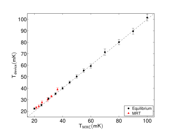
In addition to a Ruthenium Oxide thermometer mounted on the dilution refrigerator mixing chamber, the effective qubit device temperature obtained during the measurements discussed in the manuscript was determined in two independent ways. The first is based on analysis of the single-qubit Macroscopic Resonant Tunnelling (MRT) rate, and its dependence on the qubit loop flux bias $\Phi_{1x}$. Measurements and analysis of MRT rates for the devices used in this experiment are discussed in Ref 12. The second is based on measurement of the equilibrium $P_{\uparrow}$ vs. $\Phi_{1x}$ attained at fixed barrier height (fixed value of $\Phi_{2x}$). Both of these techniques are discussed in some detail in Ref. 9.

At a fixed barrier height achieved with a fixed value of $\Phi_{2x}$, the equilibrium probability $P_{\uparrow}$ approaches the thermal distribution:

$$P_{\uparrow}(t\rightarrow\infty)=\frac{1}{2}\left[\frac{1}{2}+\tanh\left(\frac{I_{p}\Phi_{1x}}{k_{B}T_{th}}\right)\right]$$ (S19)

where $I_{p}$ is the value of circulating current obtained at that value of $\Phi_{2x}$ and $T_{th}$ is the effective device temperature. Fitting a measurement of $P_{\uparrow}$ as a function of $\Phi_{1x}$ to Eq. S19, combined with a knowledge of $I_{p}$, allows us to extract $T_{th}$.

Measurement of $T_{th}$ was performed on two of the devices at each temperature setting. An average of at least two independent measurements of the device temperature $T_{th}$ of each of two qubits is compared against the mixing chamber thermometer temperature reading ($T_{MXC}$) in Figure S9. Uncertainty in $T_{th}$ was dominated by the uncertainty in the fit transition width for each measurement, which was generally found to be larger than the standard deviation of the separate measurements.

The temperature extracted from MRT transition rate widths ($T_{MRT}$) is also plotted vs. $T_{MXC}$ for temperatures below 40 mK, in Figure S9. From these plots it is clear that the two methods generally agree with each other as well as with the mixing chamber thermometer to within 3 mK over the temperature range used in the experiment.

Figure S9: Plots of $T_{th}$ (black circles) and $T_{MRT}$ (red triangles) vs. the temperature measured with the Ruthenium Oxide thermometer mounted on the mixing chamber $T_{MXC}$.

IV Quantum simulations

To obtain better quantitative understanding of the behaviour of the system, a simulation was conducted to model this experiment. The agreement between the numerical simulations can be seen in panel (b) of Fig. S2, where both percentages [experiment (theory)] are reported next to each other for each one of the low-energy conformations.

Our simulation strategy is as follows: We first write a Hamiltonian for the superconducting circuit based on standard circuit models for capacitances, inductances, and Josephson junctions. This Hamiltonian is expected to correctly describe the behaviour of coupled rf-SQUIDs. We then numerically calculate the evolution of the system based on this Hamiltonian using quantum mechanical equations of motion which take into account coupling to an environment. Therefore, we predict the quantum evolutions for the same system Hamiltonian, the same coupling to environment, and the same type of noise spectral densities. This provides a fair comparison to the experimental data.

IV.1 rf-SQUID Hamiltonian

A simplified version of the rf-SQUID qubit used in our processor is illustrated in Fig. S5a. (A more complete description of the actual qubits can be found in Ref. 3.) It has two main superconducting loops and therefore two flux degrees of freedom $\Phi_{1}$ and $\Phi_{2}$, subject to external flux biases $\Phi_{1x}$ and $\Phi_{2x}$, respectively. The Hamiltonian of such an rf-SQUID is written as

$$H_{\rm SQUID}={q_{1}^{2}\over 2C_{1}}+{q_{2}^{2}\over 2C_{2}}+U(\Phi_{1},\Phi_{2})$$ (S20)

where $C_{1}$ and $C_{2}$ are parallel and series combinations of the junction capacitances, $q_{1}$ and $q_{2}$ are the sum and difference of the charges stored in the two Josephson junctions respectively, and

$$U(\Phi_{1},\Phi_{2})={(\Phi_{1}-\Phi_{1x})^{2}/2L_{1}}+{(\Phi_{2}-\Phi_{2x})^{2}/2L_{2}}$$

$$-2E_{J}\cos(\pi\Phi_{2}/\Phi_{0})\cos(2\pi\Phi_{1}/\Phi_{0}),\qquad$$ (S21)

is a 2-dimensional potential with $L_{i}$ being the inductances of the two loops and $\Phi_{0}{=}\,h/2e$, the flux quantum. We have assumed symmetric Josephson junctions with Josephson energies $E_{J}{=}\,I_{c}\Phi_{0}/2\pi$, where $I_{c}$ is the junctions’ critical current. (A small asymmetry can be tuned away in situ in the physical implementation [3].)

At $\Phi_{1x}\approx\Phi_{0}/2$, the potential can become bistable and therefore form a two-dimensional double-well potential. If $L_{2}$ is small enough so that the deviation of $\Phi_{2}$ from $\Phi_{2x}$ can be neglected, then the two-dimensional classical potential $U(\Phi_{1},\Phi_{2})$ can be approximated by a one-dimensional double-well potential, as shown in Fig. S5b. However, with our realistic qubit parameters, $\Phi_{2}$ cannot be neglected and therefore is accounted for in all our numerical calculations. When $\Phi_{1x}=\Phi_{0}/2$, the two wells are symmetric with no energy bias between them. One can tilt the potential by changing $\Phi_{1x}$ and establish an energy bias, as depicted in Fig. S5b. It is also possible to change the barrier height by changing $\Phi_{2x}$.

An array of such qubits can be modelled by summing contributions of Eq. (S20) from each device plus terms that describe magnetic coupling of the loops:

$$H_{S}=\sum_{i}H_{\rm SQUID}^{(i)}+\sum_{i>j}H^{(ij)}_{\rm coupl}$$ (S22)

Coupling between qubits $i$ and $j$ can be modelled as a mutual inductance $M_{ij}$ between loop 1 of each pair of coupled qubits:

$$H^{(ij)}_{\rm coupl}=(\Phi^{(i)}_{1}-\Phi^{(i)}_{1x})(\Phi^{(j)}_{1}-\Phi^{(j)}_{1x})M_{ij}/L_{1}^{(i)}L_{1}^{(j)}$$ (S23)

As discussed in Section III.3 above, all parameters, i.e., inductances $L_{\alpha}^{(i)}$, capacitances $C_{\alpha}^{(i)}$, and Josephson critical currents $I_{c}^{(i)}$, are measured independently for each qubit.

To describe the system accurately we also need to introduce interaction with environment. Flux noise, which is the dominant noise in flux qubits, couples to the $i$th qubit as fluctuations $\delta\Phi_{\alpha x}^{(i)}$ of the external flux $\Phi_{\alpha x}^{(i)}$:

$$H_{\rm int}=-\sum_{\alpha=1}^{2}\sum_{i}{\Phi_{\alpha}^{(i)}-\Phi_{\alpha x}^{(i)}\over L_{\alpha}^{(i)}}\delta\Phi_{\alpha x}^{(i)}$$ (S24)

The noise is much smaller for the smaller loop $\Phi_{2x}^{(i)}$ than for the larger loop $\Phi_{1x}^{(i)}$ due to the loop size. The flux noise $\delta\Phi_{\alpha x}^{(i)}$ is assumed to be uncorrelated between the qubits, which agrees with recent experimental observation[13].

IV.1.1 Chip calibration and device parameter extraction

Device parameters were extracted for the simulations through a series of independent measurements of qubit circulating current, tunnel splitting $\Delta$, and MRT peak spacing. A discussion of how these measurements are performed is given in Ref. 3. Parameter values used in simulations are summarised in Table 3.

IV.2 Quantum Simulation

To simulate the quantum mechanical dynamics of the system, we treat (S22)-(S24) as quantum mechanical Hamiltonians. In that case, the charge $q^{(i)}_{\alpha}$ is taken to be an operator, which is the momentum conjugate to the flux operator $\Phi^{(i)}_{\alpha}$ with commutation relation: $[\Phi^{(i)}_{\alpha},q^{(i)}_{\alpha}]=i\hbar$. Unfortunately, it is impossible to calculate the dynamics of the system directly on the $2N$-dimensional continuous potential quantum mechanically. Instead, we use energy discretization as a means to simplify the calculation. The simplest way to accomplish this is to treat an rf-SQUID as a 2-state system or qubit and replace (S22) by a coupled qubit Hamiltonian. One may go further and keep more than two states per rf-SQUID in the calculation, as we shall discuss below.

We first numerically diagonalise the single rf-SQUID Hamiltonian (S20) to obtain the lowest eigenvalues and eigenvectors. We treat the lowest few energy levels as the subspace relevant for computation. We then write the Hamiltonian in the basis of states that are localised within the wells. Such states are not true eigenfunctions of the Hamiltonian and, therefore, are metastable towards tunnelling to the opposite well. Hence, the resulting Hamiltonian in such a basis will have off-diagonal terms between states in the opposite wells but not between states within each well. The latter is because those states should be stationary within their own wells; any transition (relaxation) between them is only induced by the environment.

Let $|l\rangle$ denote localised states within the wells. We use even (odd) state numbers, i.e., $l=2n$ ($2n{+}1$), with $n=0,1,2,...$, to denote states that are localised in the left (right) well. For the lowest $M$ energy levels ($M$ is taken to be even), the effective $M{\times}M$ tunnelling Hamiltonian is written as

$$H_{S}=\sum_{l=0}^{M-1}E_{l}|l\rangle\langle l|+\sum_{n,m=0}^{M/2-1}K_{2n,2m{+}1}(|2n\rangle\langle 2m{+}1|+|2m{+}1\rangle\langle 2n|)$$ (S25)

where $E_{l}$ is the energy expectation value for state $|l\rangle$ and $K_{2n,2m{+}1}$ is the tunnelling amplitude between states $|2n\rangle$ and $|2m{+}1\rangle$, which exist in opposite wells. Notice that there is no matrix element between states on the same well: $\langle 2n|H_{S}|2m\rangle=\langle 2n{+}1|H_{S}|2m{+}1\rangle=0$, which means that the states are metastable only towards tunnelling to the other side, or the states are quasi-eigenstates of the Hamiltonian within their own sides. All parameters of the tunnelling Hamiltonian, i.e., $E_{l}$ and $K_{ll^{\prime}}$ are extracted from the original rf-SQUID Hamiltonian (S20). For the 2-state qubit model we keep only the lowest two energy levels of (S25). The effective qubit Hamiltonian can be written as

$$H_{eff}=-{1\over 2}(\epsilon\sigma_{z}+\Delta\sigma_{x})$$ (S26)

where

$$\epsilon=E_{0}-E_{1},\qquad\Delta=-2K_{01},$$ (S27)

We also go beyond the 2-state model and keep 4 states per rf-SQUID. Those 4 states can be represented by two coupled qubits, one of which represents the direction of persistent current or flux, and the other one generating intrawell energy levels. We represent the first (logical) qubit by Pauli matrices $\sigma_{\alpha}$, and the extra (ancilla) qubit by Pauli matrices $\tau_{\alpha}$. The effective Hamiltonian for those two coupled qubits can be written as

$$H_{eff}=-{1\over 2}(\epsilon\sigma_{z}+\Delta\sigma_{x})+{1\over 2}[\omega_{p}\tau_{z}+\kappa_{xz}\sigma_{x}(1+\tau_{z})+\kappa_{xx}\sigma_{x}\tau_{x}].$$ (S28)

It is easy to show that (S28) is equivalent, up to a constant energy, to Hamiltonian (S25), with $M=4$, if

$$\epsilon=E_{0}-E_{1}=E_{2}-E_{3},\qquad\omega_{p}=E_{2}-E_{0}=E_{3}-E_{1},\qquad\Delta=-2K_{01},$$ (S29)

$$\kappa_{xz}=K_{23}-K_{01}\approx K_{23},\qquad\kappa_{xx}=2K_{03}=2K_{12}.$$ (S30)

As can be seen, the coupling between logical and ancilla qubits are of XX+XZ type. Coupling qubits to each other is accomplished using $\sigma_{z}$ operators which represent the direction of the induced flux. The ancilla qubits remain uncoupled from each other and from other qubits. It should be noted that the readout at the end of the evolution can only distinguish “left” well from “right” well in the double-well potential and cannot distinguish levels within each well. This is equivalent to reading out logical qubits and not ancilla qubits, but as we mentioned above, only logical qubits carry information.

Figure S10: Parameters of the 4-level model for rf-SQUID qubit as a function of time during annealing.

To properly treat the environment, we need to write the interaction Hamiltonian (S24) in the subspace of the lowest energy levels in terms of Pauli matrices. For quantum simulations we only consider noise coupling to the larger loop in Fig. S5a. Let us consider a single rf-SQUID and write the interaction Hamiltonian as

$$H_{\rm int}=-{\Phi_{1}-\Phi_{1x}\over L_{1}}\delta\Phi_{1x}$$ (S31)

We define the qubit persistent current by

$$I_{p}={1\over L_{1}}\left|\langle l|(\Phi_{1}-\Phi_{1x})|l\rangle\right|.$$ (S32)

Here, we take $I_{p}$ to be independent of $|l\rangle$ for the low lying states considered, although in reality there could be a small dependence. The interaction Hamiltonian can then be written as

$$H_{\rm int}=-{1\over 2}(\sigma_{z}+\lambda\tau_{x})Q,$$ (S33)

where

$$Q=2I_{p}\delta\Phi_{1x},\qquad\lambda={\langle 0|H_{\rm int}|2\rangle\over 2I_{p}L_{1}}={\langle 1|H_{\rm int}|3\rangle\over 2I_{p}L_{1}}$$ (S34)

The matrix elements $\langle 0|H_{\rm int}|2\rangle$ or $\langle 1|H_{\rm int}|3\rangle$ are calculated directly via Eq. S31 using the eigenfunctions of the rf-SQUID Hamiltonian, Eq. S20). The values of $I_{p}$ and $\lambda$ can therefore be calculated numerically from the original rf-SQUID Hamiltonian. Only $Q$ remains which should be characterised via its spectral density, which is the subject of Appendix A.

Quantum evolution of the system was calculated using a Markovian master equation for the density matrix described in Ref. 14. Since the evolution is very slow (adiabatic) and temperature is low, only a small number of energy levels are expected to be occupied during the evolution. We write the density matrix in the instantaneous energy eigenstate basis and truncate it to the lowest 24 energy levels, which was found to sufficiently describe the type of evolution studied here. We use both 2-state and 4-state models for rf-SQUIDs, as described above, in our simulations. The result of the 4-level model simulation is shown in Fig. S2b.

Appendix A Noise spectral density

The quantum noise operator $Q=2I_{p}\delta\Phi_{1x}$ is related to the flux noise as expected (for simplicity we only consider one rf-SQUID), and is characterised by its correlation function. Let us define the spectral density

$$S(\omega)=\int_{-\infty}^{\infty}dt\ e^{i\omega t}\langle Q(t)Q(0)\rangle=4I_{p}^{2}S_{\Phi}(\omega)$$ (S35)

where

$$S_{\Phi}(\omega)=\int_{-\infty}^{\infty}dt\ e^{i\omega t}\langle\delta\Phi_{1x}(t)\delta\Phi_{1x}(0)\rangle$$ (S36)

is the spectral density of the flux noise. No direct measurement of $S_{\Phi}(\omega)$ at all frequencies is available. We assume the spectral density is a sum of low frequency and high frequency components: $S_{\Phi}(\omega)=S_{LF}(\omega)+S_{HF}(\omega)$. For the low frequency component we use

$$S_{LF}(\omega)={(A^{2}/k_{B}T)\hbar\omega|\omega|^{-\alpha}\over 1-e^{-\hbar\omega/k_{B}T}},$$ (S37)

with $\alpha\approx 1$, which at low $\omega$ behaves as 1/f noise: $\sim A^{2}|\omega|^{-\alpha}$. Parameter $A$ is measured from low frequency noise measurement [15] and is found to be $A\approx 3$ n$\Phi_{0}$.

The high frequency parts of the spectral density is assumed to be ohmic,

$$S_{HF}(\omega)=\left({\hbar^{2}\over 4I_{p0}^{2}}\right){\eta\omega e^{-|\omega|/\omega_{c}}\over 1-e^{-\hbar\omega/k_{B}T}},$$ (S38)

where $\omega_{c}$ is the upper cutoff frequency, $\eta$ is the dimensionless coupling coefficient, and $I_{p0}$ is the value of persistent current at which $\eta$ is measured. The coupling coefficient and the persistent current are found, using Macroscopic resonant tunnelling experiment (MRT), to be $\eta\approx 0.4$ and $I_{p0}\approx 1\ \mu$A. The details of extraction of $\eta$ via MRT are presented elsewhere [12].

This leaves no free parameters for the quantum simulations.

References

- S̆ali, Shakhnovich, and Karplus [1994] A. S̆ali, E. Shakhnovich, and M. Karplus, “How does a protein fold?” Nature 369, 248–251 (1994).
- Pande [2010] V. S. Pande, “Simple theory of protein folding kinetics,” Phys. Rev. Lett. 105, 198101 (2010).
- Dill et al. [2008] K. A. Dill, S. B. Ozkan, M. S. Shell, and T. R. Weikl, “The protein folding problem,” Ann. Rev. Biophys. 37, 289–316 (2008).
- Mirny and Shakhnovich [2001] L. Mirny and E. Shakhnovich, “Protein folding theory: from lattice to all-atom models,” Annu. Rev. Biophys. Bio. 30, 361–396 (2001).
- Pande, Grosberg, and Tanaka [2000] V. S. Pande, A. Y. Grosberg, and T. Tanaka, “Heteropolymer freezing and design: Towards physical models of protein folding,” Rev. Mod. Phys. 72, 259 (2000).
- Kolinski and Skolnick [1996] A. Kolinski and J. Skolnick, Lattice Models of Protein Folding, Dynamics and Thermodynamics (Chapman & Hall, 1996).
- Shakhnovich [1994] E. I. Shakhnovich, “Proteins with selected sequences fold into unique native conformation,” Phys. Rev. Lett. 72, 3907 (1994).
- Berger and Leighton [1998] B. Berger and T. Leighton, “Protein folding in the hydrophobic-hydrophilic (HP) model is NP-complete,” J. Comput. Biol. 5, 27–40 (SPR 1998).
- Crescenzi et al. [1998] P. Crescenzi, D. Goldman, C. Papadimitriou, A. Piccolboni, and M. Yannakakis, “On the complexity of protein folding,” J. Comput. Biol. 5, 597–603 (1998).
- Hart and Istrail [1997] W. E. Hart and S. Istrail, “Robust proofs of NP-Hardness for protein folding: General lattices and energy potentials,” J. Comput. Biol. 4, 1–22 (1997).
- Yue and Dill [1995] K. Yue and K. A. Dill, “Forces of tertiary structural organization in globular proteins,” Proc. Natl. Acad. Sci. USA. 92, 146 –150 (1995).
- Miyazawa and Jernigan [1996] S. Miyazawa and R. L. Jernigan, “Residue-residue potentials with a favorable contact pair term and an unfavorable high packing density term, for simulation and threading,” Journal of Molecular Biology 256, 623–644 (1996).
- Amara, Hsu, and Straub [1993] P. Amara, D. Hsu, and J. E. Straub, “Global energy minimum searches using an approximate solution of the imaginary time schroedinger equation,” J. Phys. Chem. 97, 6715–6721 (1993).
- Finnila et al. [1994] A. B. Finnila, M. A. Gomez, C. Sebenik, C. Stenson, and J. D. Doll, “Quantum annealing: A new method for minimizing multidimensional functions,” Chem. Phys. Lett. 219, 343–348 (1994).
- Kadowaki and Nishimori [1998] T. Kadowaki and H. Nishimori, “Quantum annealing in the transverse ising model,” Phys. Rev. E. 58, 5355 (1998).
- Farhi et al. [2001] E. Farhi, J. Goldstone, S. Gutmann, J. Lapan, A. Lundgren, and D. Preda, “A quantum adiabatic evolution algorithm applied to random instances of an NP-Complete problem,” Science 292, 472–475 (2001).
- Santoro et al. [2002] G. Santoro, R. Marton k, E. Tosatti, and R. Car, “Theory of quantum annealing of an ising spin glass,” Science 295, 2427 2430 (2002), 10.1126/science.1068774.
- Brooke et al. [1999] J. Brooke, D. Bitko, T. F. Rosenbaum, and G. Aeppli, “Quantum annealing of a disordered magnet,” Science 284, 779–781 (1999).
- Santoro and Tosatti [2006] G. E. Santoro and E. Tosatti, “Optimization using quantum mechanics: quantum annealing through adiabatic evolution,” J. Phys. A. 39, R393–R431 (2006).
- Das and Chakrabarti [2008] A. Das and B. K. Chakrabarti, “Colloquium: Quantum annealing and analog quantum computation,” Rev. Mod. Phys. 80, 1061 21 (2008).
- Kirkpatrick, Gelatt, and Vecchi [1983] S. Kirkpatrick, C. D. Gelatt, and M. P. Vecchi, “Optimization by simulated annealing,” Science 220, 671–680 (1983).
- Bohannon [2005] J. Bohannon, “Distributed computing: Grassroots supercomputing,” Science 308, 810 (2005).
- Shaw et al. [2010] D. E. Shaw, P. Maragakis, K. Lindorff-Larsen, S. Piana, R. O. Dror, M. P. Eastwood, J. A. Bank, J. M. Jumper, J. K. Salmon, Y. Shan, and W. Wriggers, “Atomic-Level characterization of the structural dynamics of proteins,” Science 330, 341–346 (2010).
- Li et al. [2010] M. S. Li, N. T. Co, G. Reddy, C.-K. Hu, J. E. Straub, and D. Thirumalai, “Factors governing fibrillogenesis of polypeptide chains revealed by lattice models,” Phys. Rev. Lett. 105, 218101 (2010).
- Perdomo et al. [2008] A. Perdomo, C. Truncik, I. Tubert-Brohman, G. Rose, and A. Aspuru-Guzik, “Construction of model hamiltonians for adiabatic quantum computation and its application to finding low-energy conformations of lattice protein models,” Phys. Rev. A 78, 012320–15 (2008).
- Johnson et al. [2011] M. W. Johnson, M. H. S. Amin, S. Gildert, T. Lanting, F. Hamze, N. Dickson, R. Harris, A. J. Berkley, J. Johansson, P. Bunyk, E. M. Chapple, C. Enderud, J. P. Hilton, K. Karimi, E. Ladizinsky, N. Ladizinsky, T. Oh, I. Perminov, C. Rich, M. C. Thom, E. Tolkacheva, C. J. S. Truncik, S. Uchaikin, J. Wang, B. Wilson, and G. Rose, “Quantum annealing with manufactured spins,” Nature 473, 194–198 (2011).
- Farhi et al. [2000] E. Farhi, J. Goldstone, S. Gutmann, and M. Sipser, “Quantum computation by adiabatic evolution,” arXiv:quant-ph/0001106 (2000).
- Hogg [2003] T. Hogg, “Adiabatic quantum computing for random satisfiability problems,” Phys. Rev. A. 67, 022314 (2003).
- Steffen et al. [2003] M. Steffen, W. van Dam, T. Hogg, G. Breyta, and I. Chuang, “Experimental implementation of an adiabatic quantum optimization algorithm,” Phys. Rev. Lett. 90, 067903 (2003).
- Xu et al. [2011] N. Xu, J. Zhu, D. Lu, X. Zhou, X. Peng, and J. Du, “Quantum factorization of 143 on a dipolar-coupling nmr system,” arXiv:1111.3726v1 (2011).
- Wernsdorfer [2010] W. Wernsdorfer, “Molecular nanomagnets: towards molecular spintronics,” Int. J. Nanotechnol. 7, 497 – 522 (2010).
- Vion et al. [2002] D. Vion, A. Aassime, A. Cottet, P. Joyez, H. Pothier, C. Urbina, D. Esteve, and M. H. Devoret, “Manipulating the quantum state of an electrical circuit,” Science 296, 886–889 (2002).
- You and Nori [2005] J. Q. You and F. Nori, “Superconducting circuits and quantum information.” Phys. Today. 58, 42–47 (2005).
- Lupascu et al. [2007] A. Lupascu, S. Saito, T. Picot, P. C. de Groot, C. J. P. M. Harmans, and J. E. Mooij, “Quantum non-demolition measurement of a superconducting two-level system,” Nat. Phys. 3, 119–125 (2007).
- Hofheinz et al. [2009] M. Hofheinz, H. Wang, M. Ansmann, R. C. Bialczak, E. Lucero, M. Neeley, A. D. O’Connell, D. Sank, J. Wenner, J. M. Martinis, and A. N. Cleland, “Synthesizing arbitrary quantum states in a superconducting resonator,” Nature 459, 546–549 (2009).
- DiCarlo et al. [2009] L. DiCarlo, J. M. Chow, J. M. Gambetta, L. S. Bishop, B. R. Johnson, D. I. Schuster, J. Majer, A. Blais, L. Frunzio, S. M. Girvin, and R. J. Schoelkopf, “Demonstration of two-qubit algorithms with a superconducting quantum processor,” Nature 460, 240–244 (2009).
- Neeley et al. [2010] M. Neeley, R. C. Bialczak, M. Lenander, E. Lucero, M. Mariantoni, A. D. O/’Connell, D. Sank, H. Wang, M. Weides, J. Wenner, Y. Yin, T. Yamamoto, A. N. Cleland, and J. M. Martinis, “Generation of three-qubit entangled states using superconducting phase qubits,” Nature 467, 570–573 (2010).
- DiCarlo et al. [2010] L. DiCarlo, M. D. Reed, L. Sun, B. R. Johnson, J. M. Chow, J. M. Gambetta, L. Frunzio, S. M. Girvin, M. H. Devoret, and R. J. Schoelkopf, “Preparation and measurement of three-qubit entanglement in a superconducting circuit,” Nature 467, 574–578 (2010).
- Kaminsky, Lloyd, and Orlando [2004] W. M. Kaminsky, S. Lloyd, and T. P. Orlando, “Scalable superconducting architecture for adiabatic quantum computation,” arXiv:quant-ph/0403090 (2004).
- Bian et al. [2012] Z. Bian, F. Chudak, W. G. Macready, L. Clark, and F. Gaitan, “Experimental determination of ramsey numbers with quantum annealing,” arXiv:1201.1842v2 (2012).
- Harris et al. [2010] R. Harris, M. W. Johnson, T. Lanting, A. J. Berkley, J. Johansson, P. Bunyk, E. Tolkacheva, E. Ladizinsky, N. Ladizinsky, T. Oh, F. Cioata, I. Perminov, P. Spear, C. Enderud, C. Rich, S. Uchaikin, M. C. Thom, E. M. Chapple, J. Wang, B. Wilson, M. H. S. Amin, N. Dickson, K. Karimi, B. Macready, C. J. S. Truncik, and G. Rose, “Experimental investigation of an eight-qubit unit cell in a superconducting optimization processor,” Phys. Rev. B. 82, 024511 (2010).
- Barahona [1982] F. Barahona, “On the computational complexity of ising spin glass models,” J. Phys. A: Math. Gen. 15, 3241–3253 (1982).
- Anfinsen [1973] C. B. Anfinsen, “Principles that govern the folding of protein chains,” Science 181, 223–230 (1973).
- Lau and Dill [1989] K. F. Lau and K. A. Dill, “A lattice statistical-mechanics model of the conformational and sequence-spaces of proteins,” Macromolecules. 22, 3986–3997 (1989).
- Perdomo-Ortiz, O’Gorman, and Aspuru-Guzik [2011] A. Perdomo-Ortiz, B. O’Gorman, and A. Aspuru-Guzik, “Construction of energy functions for self-avoiding walks and the lattice heteropolymer model: resource efficient encoding for quantum optimization,” In preparation (2011).
- Amin, Truncik, and Averin [2009] M. H. S. Amin, C. J. S. Truncik, and D. V. Averin, “Role of single-qubit decoherence time in adiabatic quantum computation,” Phys. Rev. A 80, 022303 (2009).
- Amin, Averin, and Nesteroff [2009] M. H. S. Amin, D. V. Averin, and J. A. Nesteroff, “Decoherence in adiabatic quantum computation,” Phys. Rev. A 79, 022107 (2009).
- Camacho and Thirumalai [1993] C. J. Camacho and D. Thirumalai, “Minimum energy compact structures of random sequences of heteropolymers,” Phys. Rev. Lett. 71, 2505–2508 (1993).
- Hartmann and Rieger [2004] A. K. Hartmann and H. Rieger, New Optimization Algorithms in Physics (Wiley-VCH, 2004).
- Harris et al. [2010a] R. Harris, J. Johansson, A. J. Berkley, M. W. Johnson, T. Lanting, S. Han, P. Bunyk, E. Ladizinsky, T. Oh, I. Perminov, E. Tolkacheva, S. Uchaikin, E. M. Chapple, C. Enderud, C. Rich, M. Thom, J. Wang, B. Wilson, and G. Rose, “Experimental demonstration of a robust and scalable flux qubit,” Phys. Rev. B 81, 134510 (2010a).
- Johnson et al. [2010] M. W. Johnson, P. Bunyk, F. Maibaum, E. Tolkacheva, A. J. Berkley, E. M. Chapple, R. Harris, J. Johansson, T. Lanting, I. Perminov, E. Ladizinsky, T. Oh, and G. Rose, “A scalable control system for a superconducting adiabatic quantum optimization processor,” Supercond. Sci. Tech. 23, 065004 (2010).
- Harris et al. [2009a] R. Harris, T. Lanting, A. J. Berkley, J. Johansson, M. W. Johnson, P. Bunyk, E. Ladizinsky, N. Ladizinsky, T. Oh, and S. Han, “Compound Josephson-junction coupler for flux qubits with minimal crosstalk,” Phys. Rev. B 80, 052506 (2009a).
- Harris et al. [2010b] R. Harris, M. W. Johnson, T. Lanting, A. J. Berkley, J. Johansson, P. Bunyk, E. Tolkacheva, E. Ladizinsky, N. Ladizinsky, T. Oh, F. Cioata, I. Perminov, P. Spear, C. Enderud, C. Rich, S. Uchaikin, M. C. Thom, E. M. Chapple, J. Wang, B. Wilson, M. H. S. Amin, N. Dickson, K. Karimi, B. Macready, C. J. S. Truncik, and G. Rose, “Experimental investigation of an eight-qubit unit cell in a superconducting optimization processor,” Phys. Rev. B 82, 024511 (2010b).
- Harris et al. [2009b] R. Harris, F. Brito, A. J. Berkley, J. Johansson, M. W. Johnson, T. Lanting, P. Bunyk, E. Ladizinsky, B. Bumble, A. Fung, A. Kaul, A. Kleinsasser, and S. Han, “Synchronization of multiple coupled rf-SQUID flux qubits,” New J. Phys. 11, 123022 (2009b).
- Harris et al. [2008] R. Harris, M. W. Johnson, S. Han, A. J. Berkley, J. Johansson, P. Bunyk, E. Ladizinsky, S. Govorkov, M. C. Thom, S. Uchaikin, B. Bumble, A. Fung, A. Kaul, A. Kleinsasser, M. H. S. Amin, and D. V. Averin, “Probing noise in flux qubits via macroscopic resonant tunneling,” Phys. Rev. Lett. 101, 117003 (2008).
- Harris et al. [2009c] R. Harris, A. Berkley, J. Johansson, M. Johnson, T. Lanting, P. Bunyk, E. Tolkacheva, E. Ladizinsky, B. Bumble, A. Fung, A. Kaul, A. Kleinsasser, and S. Han, “Implementation of a quantum annealing algorithm using a superconducting circuit,” arXiv:0903.3906v1 (2009c).
- Berkley et al. [2010] A. J. Berkley, M. W. Johnson, P. Bunyk, R. Harris, J. Johansson, T. Lanting, E. Ladizinsky, E. Tolkacheva, M. H. S. Amin, and G. Rose, “A scalable readout system for a superconducting adiabatic quantum optimization system,” Supercond. Sci. Tech. 23, 105014 (2010).
- Lanting et al. [2004] T. Lanting, M. Amin, M. Johnson, F. Altomare, A. Berkley, S. Gildert, R. Harris, J. Johansson, P. Bunyk, E. Ladizinsky, E. Tolkacheva, and D. Averin, “Probing high frequency noise with macroscopic resonant tunneling,” arXiv:1103.1931v1 (2004).
- Lanting et al. [2010] T. Lanting, R. Harris, J. Johansson, M. H. S. Amin, A. J. Berkley, S. Gildert, M. W. Johnson, P. Bunyk, E. Tolkacheva, E. Ladizinsky, N. Ladizinsky, T. Oh, I. Perminov, E. M. Chapple, C. Enderud, C. Rich, B. Wilson, M. C. Thom, S. Uchaikin, and G. Rose, “Cotunneling in pairs of coupled flux qubits,” Phys. Rev. B 82, 060512 (2010).
- Lanting et al. [2009] T. Lanting, A. J. Berkley, B. Bumble, P. Bunyk, A. Fung, J. Johansson, A. Kaul, A. Kleinsasser, E. Ladizinsky, F. Maibaum, R. Harris, M. W. Johnson, E. Tolkacheva, and M. H. S. Amin, “Geometrical dependence of the low-frequency noise in superconducting flux qubits,” Phys. Rev. B 79, 060509(R) (2009).