, ,
Selective sweeps in growing microbial colonies
Abstract
Evolutionary experiments with microbes are a powerful tool to study mutations and natural selection. These experiments, however, are often limited to the well-mixed environments of a test tube or a chemostat. Since spatial organization can significantly affect evolutionary dynamics, the need is growing for evolutionary experiments in spatially structured environments. The surface of a Petri dish provides such an environment, but a more detailed understanding of microbial growth on Petri dishes is necessary to interpret such experiments. We formulate a simple deterministic reaction-diffusion model, which successfully predicts the spatial patterns created by two competing species during colony expansion. We also derive the shape of these patterns analytically without relying on microscopic details of the model. In particular, we find that the relative fitness of two microbial strains can be estimated from the logarithmic spirals created by selective sweeps. The theory is tested with strains of the budding yeast Saccharomyces cerevisiae, for spatial competitions with different initial conditions and for a range of relative fitnesses. The reaction-diffusion model also connects the microscopic parameters like growth rates and diffusion constants with macroscopic spatial patterns and predicts the relationship between fitness in liquid cultures and on Petri dishes, which we confirmed experimentally. Spatial sector patterns therefore provide an alternative fitness assay to the commonly used liquid culture fitness assays.
pacs:
87.23.Kg, 87.23.Cc, 87.18.Hf, 87.18.TtKeywords: Fisher waves, wave velocity, selective sweep, competition at the front, spatial assay, relative fitness
1 Introduction
Traditionally, the theory of evolution has been developed by analyzing phenotypes and genotypes found in natural populations and fossil records [1, 2]. However, due to recent developments in microbiology and modern genetics, evolutionary experiments are becoming a valuable research tool [3]. Laboratory experiments hold great promise for uncovering basic evolutionary mechanisms by allowing us to observe evolution over time. More important, experiments, unlike evolution in natural populations, can be repeated systematically to distinguish between general principles and historical accidents. Microbes are particularly suited for evolutionary studies because they are relatively simple, reproduce and evolve rapidly, and can be easily modified using genetic engineering. Experiments with microorganisms could also provide insights into tumor growth, the spread of antibiotic resistance, and directed evolution of microbes to produce medicines or biofuels [4, 5].
One potential drawback of evolutionary experiments is that they are conducted in artificial laboratory environments, which are quite different from the natural ecology of the species studied. The choice of the laboratory environment is therefore very important because it could affect both the nature of observed adaptations and the evolutionary dynamics. Most microbial experiments, of interest to us here, are conducted in the well-mixed environments of a chemostat or a test tube. These well-controlled environments allow researchers to compare experimental results to theoretical predictions, but it is important to ensure that such results are generic, not environment specific. Spatial structure, absent in well-mixed cultures, can significantly affect evolutionary dynamics [6, 7, 8, 9, 10]; therefore, it is important to carry out experiments with growth conditions that allow spatial inhomogeneities to form. The surface of a Petri dish is an easy-to-use environment, chemically similar to the environments of a test tube or a chemostat, yet capable of sustaining and preserving spatial structure during colony growth. Recently, several studies have used microorganisms in Petri dishes to study spatial patterning, mutations, and evolution [11, 12, 13, 4, 14, 15, 8, 16, 17, 18, 19, 20, 21, 22]. Our focus here is on compact growth of colonies containing different genetic variants. For a comprehensive review emphasizing the beautiful dendritic growth patterns that can arise at low nutrient concentrations see Ref. [23].
An important obstacle to a wider use of spatial environments in evolutionary experiments is the limited theoretical understanding of how basic evolutionary processes play out in a spatial context. In particular, one must have a way to measure fitness to study evolution, but there are few models that relate microscopic parameters of the organisms to macroscopic quantities that can be easily measured in the laboratory. In this paper, we formulate a coarse-grained model of spatial competition that fills this gap and carry out microbial experiments to test the model’s predictions. This model is based on deterministic reaction-diffusion equations, which describe short-range migration of the organisms and their competition. Our numerical results are further supported by a geometric argument, which does not rely on the detailed assumptions about microbial growth and migration. Stochastic effects due to number fluctuations (genetic drift) can be included in the model [15, 24, 25], but they do not play a central role in our analysis and are neglected for simplicity. For a study of spatial competition between two neutral bacterial strains, which is dominated by genetic drift, see Ref. [17]. Although we focus on competitions, the model is sufficiently general to describe mutualistic and antagonistic interactions as well.
Compared to well-mixed populations, spatial populations have a wide range of initial conditions because one has to specify not only the relative fractions of genotypes but also their spatial distribution at time zero. We examine several experimentally interesting initial conditions and calculate how the spatial distributions of genotypes changes with time. We find that the shape of the resulting spatio-genetic patterns is determined by the expansion velocities ratio , where and are the expansion velocities of isolated colonies composed exclusively of strain or strain . Relative fitnesses of the genotypes can then be estimated by comparing experimentally observed spatio-genetic patterns to the theory. In particular, the selective advantage in this context can be defined as . As we show below, this definition is closely related to the traditional definition in terms of exponential growth rates. For linear inoculations, our results in the long time limit agree with Ref. [24], where a phenomenological model of the patterns was first proposed. In contrast to Ref. [24], we also study circular inoculations and carry out experiments to test quantitative predictions of our model.
The theory can be directly compared to the experiments because the spatial distribution of genotypes on a Petri dish can be visualized and quantified with fluorescent markers [15]. Here, we briefly describe this technique; see the supplementary information (section S1) for more details. Microbial strains of interest are genetically modified to constitutively produce a fluorescent protein. The emission spectra of the proteins must be sufficiently different in order to distinguish the strains on a Petri dish. To study selective sweeps, a mixture of the strains is prepared in liquid medium, usually with the fitter strain in the minority. A drop of this mixture is then deposited on a small region of a Petri dish with solid growth medium. Different shapes of this drop lead to different initial conditions. Circular drops are naturally created by the surface tension forces when small drops of fluid are placed on a Petri dish. Linear drops can be created by gently touching the surface of the medium with a razor blade after dipping it in the mixture of the strains. These drops dry quickly, and microbial colonies start to grow, expanding by about a centimeter a week. The spatial distribution of genotypes can be observed during this expansion by fluorescent microscopy, as shown in figure 1.
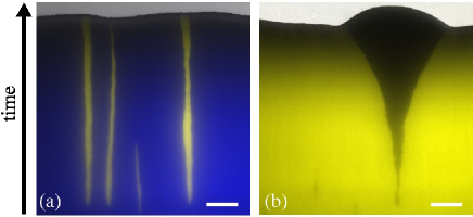
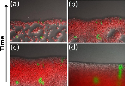
Sectors in figure 1 are at the center of this study. In our experiments, cells are nonmotile and grow primarily at the expanding frontier; behind the front, the growth is limited by the lack of nutrients [27, 28]. As a result, the genetic composition in the interior of the colony does not change with time. The spatio-genetic pattern shown in figure 1 is then a frozen record of the temporal changes in the spatial distribution of genotypes at the expanding frontier. In figure 1a, we show growth of two strains with the same fitness that differ only in the colour of a fluorescent marker. Before deposition on the Petri dish, these strains were combined in a 1:50 ratio and thoroughly mixed. However, the two different colours (genotypes) demix and form sectors. This demixing is caused by number fluctuations (genetic drift) at the expanding edge [15, 6]. One can see this stochastic process at the resolution of a single cell (m in diameter) in figure 2. In contrast to neutral demixing, figure 1b shows sector formation in a colony founded by two strains with different fitnesses; the fitter strain is in the minority initially. Over time, the fitter strain displaces the other strain, increasing its share of the expanding frontier. This expansion is also subject to number fluctuations, which are responsible for the sector boundary wiggles, but the average shape of the sector is determined primarily by the deterministic force of natural selection. For the purpose of measuring relative fitness, the effects of genetic drift can be averaged out, given a sufficient number of repeated experiments. Our deterministic model strives to describe this average sector shape and is not capable of describing the randomness in boundary motion or the dynamics when the number of the fitter organisms is so small that the number fluctuations can lead to their extinction, an effect discussed in Ref. [24].
This paper is organized as follows. We formulate a competition model assuming a well-mixed environment, such as a mechanically shaken test tube, in Sec. 2. Under these conditions, a particular microbe visits virtually every region of the carrier fluid in a cell division time, and the system is effectively “zero-dimensional.” This model is then extended to account for lateral migrations during a range expansion in Sec. 3. In Sec. 4, we analytically derive the spatial patterns created by two-species competition (including results for colliding circular colonies) using a very general argument, which does not rely on the microscopic details of microbial growth and migration. The theoretical predictions are then compared to experiments in Sec. 5. Concluding remarks are contained in Sec. 6. The supplementary information (section S1) contains the experimental and numerical methods as well as additional data supporting our conclusions.
2 Modeling competition in a well-mixed environment
A competition experiment is a standard way to measure relative fitness of two microbial strains in a well-mixed environment. During a competition experiment, the stains are introduced into a fresh medium, and their relative abundance is measured over time. Initially, the number of cells grows exponentially, but the growth eventually slows down as the system approaches the stationary phase due to crowded conditions. This behavior is captured by a simple Lotka-Volterra-type model [29]:
| (1) |
which is the most general model with quadratic nonlinearities. Here, and are the concentrations (number of cells per unit volume) of strain and strain respectively. The constants and are their exponential growth rates; and the constant matrix describes nonlinear interactions. For a mono-culture consisting of a single yeast strain, Refs. [30, 31] showed that population growth can be described by the logistic equation (i.e. with quadratic nonlinearities) very accurately.
By rescaling and , we can recast equation (1) in a slightly more convenient form
| (2) |
where and , and we use the same symbols and for the rescaled concentrations. When , we shall say that the competition takes place “under crowded conditions”. Our notation emphasizes that the initial stage of exponential growth is usually much shorter than the second phase of competition under crowded conditions, i.e. the growth rates and , are typically much larger than the small quantities and . When , strain grows faster in the presence of the other strain, e.g. by feeding off an excess production of a useful amino acid. When , strain grows slower in the presence of the other strain, e.g., because of a secreted poison.
Note that equations (2) always have at least three fixed points: , , and . In addition, for some values of the parameters, there is another fixed point in the physically relevant domain of nonnegative and . The fixed point at the origin is always unstable.
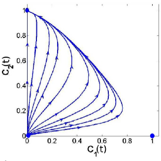
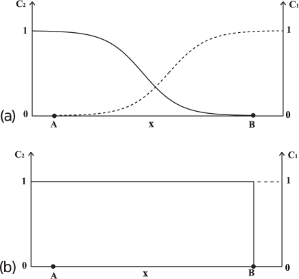
Five different behaviors are possible depending on the values of and ; four of these are illustrated in figure 3. If and are positive, the interaction of the species is mutualistic (i.e. the presence of the first strain helps the second strain grow and vice versa) and leads to a single stable fixed point with a nonzero concentration of both strains. Since the focus of this paper is on competition, we do not pursue this cooperative possibility further here. If and are negative, there are two stable fixed points: one with and , the other with and . The system reaches one of these fixed points depending on which strain is more prevalent initially. An incoming separatrix divides the phase space in two domains of attraction and feeds into an unstable fixed point with and . If and , there is only one stable fixed point and . Similarly, and is the only stable fixed point when and . Finally, there is a degenerate case when the dynamics is determined only by the logistical growth. In this case, depending on the initial conditions, the system lands somewhere along the line of neutral fixed points defined by .
Interestingly, when , the ultimate result of the competition is independent of the exponential growth rates and . The dynamical path, however, does depend on these parameters. For example, for and (the situation of particular interest to us here), initially increases, but eventually falls off as the total population density rises settling at , see figure 4. This behavior has important implications for the competition at the frontier of a colony expanding in space, where the concentration of cells is always low. We show in Sec. 3 that the outcome of a spatial competition experiment is determined primarily by the exponential growth rates and rather than and , in contrast to the aforementioned behavior in a well-mixed population.
3 Competition and migration
In this section, the competition model formulated in Sec. 2 is generalized to spatially extended environments. To this end, we need a model of cell migration. In general, cell migration is a complicated process, which could involve chemotaxis333Chemotaxis is an ability of cells to direct their motion in response to a chemical signal, e.g. food or toxins., swarming, and random wandering. Although all of these can be important biologically, some can be neglected in appropriately designed spatial competition experiments. For example, cells of Baker’s yeast, Saccharomyces cerevisiae, often used in microbiological experiments, are nonmotile, and many bacterial cells, e.g. Escherichia coli, can be prevented from swimming by eliminating functioning flagella or using a high concentration of the gelation agent in the growth medium.
For nonmotile microbes, the only mechanism of cell migration is cells’ pushing on each other as they increase in size before cell division. Even a cell division of an isolated cell leads to migration because at least one of the offspring is generally displaced in a random direction relative to the position of its parent. At the colony front, where cells are relatively free to move, cell migration can be approximated by a random-walk-type process caused by growing cells pushing each other in random directions. The diffusion constant of such random walks must depend on the local concentration of cells because sector boundaries in the interior of a colony like the ones shown in figure 1 do not change with time [15]. For a concentration-independent diffusion constant, the boundaries would slowly disappear as cells of different colours gradually mix [24]; therefore, migration must be arrested at high cell concentrations. A possible mechanism of this arrest is a significant reduction in growth rate due to nutrient depletion. At the edge of the colony, however, the cell density is low, and cells move readily due to the jostling caused by cell growth, as is evident from the wandering of the sector boundaries.
Since the exact dependence of the spatial diffusion constant on the local cell concentration is unknown, we have explored a family of functional forms, namely
| (3) |
where is the diffusion constant of the first strain in the limit of small local cell concentration, and is an adjustable parameter that allows us to explore the sensitivity to rapid variations in the rate of migration near the frontier. Here, and are cell densities per unit area, rescaled as in Sec. 2. An analogous dependence, , is assumed for the second strain; here is the Heaviside step function, , and otherwise. The choice of a monotonic dependence of the diffusion constants on cell density is motivated by the monotonically decreasing supply of nutrients from the outside to the inside of the colony. To check whether a non-monotonic dependence would affect our results, we also explored . Although the speed of population waves is different in this model, the shape of spatial patterns and their connection to relative fitness remain the same; see supplementary information (section S4).
Our model of spatial competition then takes the following form
| (4) |
(a)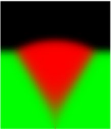
|
(b)
|

The initial and boundary conditions are chosen to mimic selective sweeps in microbial colonies. For example, in figure 5, only a very small region is initially occupied by the advantageous genotype, which corresponds to the time when a sector begins to appear in figure 1b. Our model cannot describe the earlier part of the range expansion when number fluctuations are important, because equations (4) are deterministic and treat the cell densities as continuous functions. During this early stage, the advantageous genotype becomes extinct stochastically everywhere but a few spatial locations, where it gives rise to small sectors. These sectors can then be used as the initial condition in our deterministic model. We solve equations (4) numerically; see the supplementary information (section S1) and figures 5 and 6. Note that our model of range expansions has two spatial dimensions, while, in experiments, colonies also gradually thicken in the direction perpendicular to the plate [32]. We neglect this gradual thickening here.
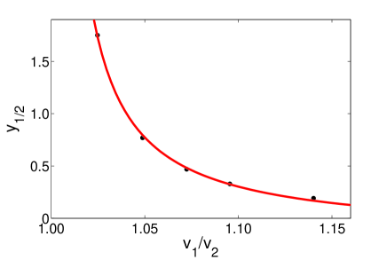
From figures 1b and 5, one can see that there are at least two stages in the sector formation. During the late stage, the two sector boundaries are far apart, and the interior of the sector is dominated by the advantageous strain. At this stage, the sector boundaries maintain a constant angle with the direction of the expansion, which we explain in Sec. 4 using a very general geometric argument. During the early stage, the size of the sector is comparable to the width of sector boundaries, and the two boundaries interact. By neglecting the nonlinear terms in equations (4) near the frontier, where and are small, we can qualitatively understand how the duration of the first stage depends on the relative fitness when the fitness difference is small (see figure 7). In this case, we can neglect the bulging of the sector and assume that the population wave front is approximately flat. For simplicity, we also assume . The -axis is taken to be along the front and the -axis to be perpendicular to the front. For the Fisher equation [33], a steady state is reached in a frame co-moving with the population wave ( and ) when only the second strain is present. In this reference frame, (note that the nonlinear terms are neglected). Since the fitness difference and the concentration of the first strain are small, the dynamics of the second strain along the -axis is approximately unchanged. Moreover, since the spatial distribution of the first strain along the -axis is the same as that of the second strain, a similar equality holds for the first strain . Upon using these two observations and the linearized version of equations (4), we find that the dynamics of the first strain near the frontier is approximately given by a linear diffusion equation with a source,
| (5) |
Note that this equation is invariant with respect to translations along , so we can treat the frontier as a quasi-one-dimensional population. For , corresponding to a point-like inoculant at the frontier, the solution of equation (5) is
| (6) |
Therefore, the characteristic time necessary for the first strain to dominate the sector scales as . This divergent time scale is indeed observed in the numerical solutions; see figure 7.
The dependence of spatial patterns during two-species competition on various parameters in equation (4) was investigated in the context of linear expansions. We varied the exponents and by factors of , ; the diffusion constants and by factors of , ; and the growth rates and by factors of , with . The competition parameters and were independently varied relative to , . This numeric exploration helped us identify important parameter combinations that control the shape of spatial patterns. We now turn to the discussion of these results.
From numerical analysis, we made an important observation that the expansion velocity of a strain growing in the absence of the other strain depends only on the exponential growth rate and diffusion constant right at the frontier and is given by
| (7) |
independent of (see supplementary information section S4) and in agreement with the classic Fisher-Kolmogorov wave theory [33, 34], which provides an exact solution for a simpler model with concentration-independent diffusivity. This agreement is not surprising because the speed of a Fisher population wave is determined only by the dynamics at the foot of the wave front [33, 29], and equation (3) ensures that the diffusivity approaches a constant for small . The intuition behind equation (7) is that the wave speed depends both on the growth rate () and on the rate of undirected migration () that brings cells to unoccupied territories. The detailed shape of the wave front, however, does depend on parameters such as and (or and ). The parameters and are irrelevant when only one strain is present because in this case.
Even when both strains are present, the knowledge of expansion velocities and is sufficient to describe the major (large scale) features of the resulting spatio-genetic pattern. To see this, note that the behavior of population fronts far from the sector boundaries is the same as when only one strain is present because the concentration of the other strain vanishes away from the boundaries. We also found that the initial position of the sector boundaries is determined only by and (and independent of and ) because, at the tip of the advancing front, the product is exponentially small compared to and . On smaller length scales of the order (or ), all parameters play a role. In particular, all parameters affect the shape of concentration profiles and the position of sector boundaries during the early stage of sector formation.
Note that, with nonzero and , sector boundaries still move behind the wave front even though the diffusivity is zero. To understand this motion, consider strains with and . The first strain expands faster, but, after the front has passed, the dynamics under crowded conditions, discussed in Sec. 2, favors the second strain. As a result, any region with a nonzero concentration of the second strain is eventually colonized by it. This behind-the-front competition should lead to a finite displacement of the boundary because every sector boundary has a finite width due to the discreteness of the number of organisms; see figure 8. Since, for many microbial strains, the boundary width is small, and , we do not expect to observe this type of sector boundary displacement (very different from a Fisher genetic wave) experimentally.
What is the relation between and relative fitness in liquid cultures? In well-mixed populations, selective advantage is often defined from the ratio of exponential growth rates, . At expanding frontiers, we define by analogy. There may not be a direct correspondence between and because the former involves diffusion constants and in addition to the growth rates and . For example, a mutation providing a means of motility could be beneficial in a Petri dish (due to faster spreading) and deleterious in liquid (due to its metabolic cost). However, two special cases and (with ) are of interest.
Equal diffusion constants should be a good approximation for mutations that affect growth rate, but do not affect motility directly, which is possible when motility does not depend on the growth rate strongly. Growth independent motility was, e.g., observed in swimming Bacillus subtilis cells [11]. Under these assumptions, , and for ; see equation (7). The other possibility could be a good approximation when motility and growth are strongly linked. For example, colonies of S. cerevisiae studied here expand due to cell growth, and it is reasonable to assume that , where is the average cell size. In this case, , as follows from equation (7); see figure 9.
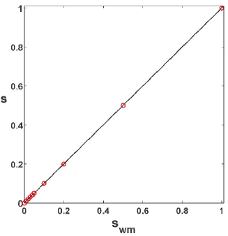 |
Our simple definition of () has three advantages: expansion velocities can be easily measured, larger expansion velocity results in greater colonized territory and, therefore, greater access to nutrients, and the ratio is closely related to the traditional definition of obtained from the exponential phase of well-mixed cultures.
In summary, the main conclusion of the mechanistic modeling embodied by equation (4) is that the essential features of spatio-genetic patterns formed during range expansion are insensitive to the details of the model and are determined by a single dimensionless parameter (the ratio of expansion velocities). We further support this conclusion in the next section by deriving the shapes of the spatial pattern without relying on the microscopic dynamics of growth and migration. Additional tests of the robustness of our reaction-diffusion model to changes in the modeling assumptions (such as varying the form of the concentration-dependent diffusion constants) are presented in section S4 of the supplementary materials.
4 Sector shapes and the equal-time argument
In this section, we develop an analytic argument to understand selective sweeps and explore different ways of measuring relative fitness from macroscopic competition experiments. This argument relies on two assumptions: the strains expand with constant velocities and a patch occupied by one strain is impenetrable to the other strain. We primarily focus on two experimental geometries: linear and circular.
4.1 Linear inoculations
Upon establishment, i.e. when sector boundaries are sufficiently far apart, the sectors from a linear inoculation have a triangular shape. Following Ref. [24], we explain this shape by the simple equal-time argument illustrated in figure 10: It should take the same amount of time for the second (less fit) strain to grow along the expansion direction as it takes the fitter first strain to grow a longer distance along the boundary. More generally, for any point along the front, we can define a length that is the length of the shortest path connecting this point and the origin of the expansion and lying entirely in the territory occupied by the same strain. (This path is a straight line for linear inoculations, but curved for radial ones, as we show below.) Then, the ratio of and the appropriate expansion velocity is the time necessary to form this particular spatial pattern. This time is the age of the colony since inoculation and must be the same for all points along the front. From this observation (see figure 10), we conclude that the bulging shape of an advantageous sector is an arc of a circle of radius and angle given by
| (8) |
which is equivalent to the result obtained in Ref. [24].
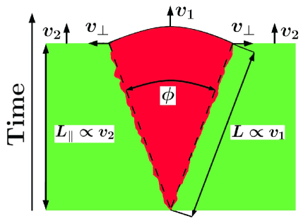
Our arguments are somewhat analogous to the Huygens-Fresnel principle in optics [36]. Each point along the front has a potential to create an outgoing circular population wave that spreads with velocity or , and unoccupied territories are colonized by the strain that gets there first. Unlike in optics, this principle can only be used to construct wave fronts at infinitesimal time steps because, once a region is colonized by one strain, it becomes impenetrable to the other strain.
The equal-time argument breaks down on length scales smaller than because the Fisher velocity will in general depend on the curvature of the wave front. For example, advancing a circular front requires more time than advancing a linear front because more cell divisions are necessary to cover the larger area colonized by the curved front. The Fisher velocity approaches the limiting value, equation (7), provided the local radius of curvature is much larger than [29]. is also the characteristic width of a sector boundary, where the equal-time argument breaks down because the strains are intermixed.
4.2 Circular expansions
We now turn to radial range expansions, resulting from moderate-sized circular pioneer populations, e.g., created by placing a drop of the inoculant on the surface of a Petri dish. Due to surface tension, small drops (of order to mm in diameter) are naturally circular. A precisely defined initial shape is a significant advantage over linear geometries susceptible to front undulations. This advantage is further strengthened because a two-dimensional reaction-diffusion population wave started from an irregular island of cells becomes more and more circular as the expansion continues. Even more important, the interactions of yeast cells lead to an effective surface tension suppressing front undulations [32].
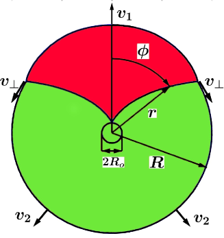
The equal-time argument also yields the shape of sectors in the circular geometry; see the schematic plot (figure 11) and numerical solution of equation (4) (figure 6). Equating the infinitesimal time increments along the radius of the wild-type colony and the curved sector boundary leads to a differential equation:
| (9) |
formulated in polar coordinates with the origin at the center of the expansion. The solution reads
| (10) |
where the different signs corresponds to boundaries turning clockwise and counterclockwise, and is the initial radius of the population. Thus, we can identify sector boundaries in microbiology with the famous logarithmic spiral of Bernoulli, which also describes the Nautilus shell and insect flight patterns [37].
The shape of the bulge at the frontier can also be calculated with the equal-time argument. The top of the bulge, well away from the sector boundaries, is a circular arc of radius centered on the origin of the sector; the angular length of this region (see figure 12) is given by
| (11) |
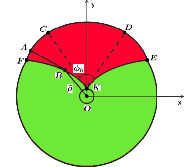
just as in the linear geometry. Beyond , the bulge is closer to the sector origin than because these points along the bulge cannot be connected to the origin of the sector by a straight line without intersecting the territories occupied by the other strain. In this case, the shortest allowed path back to the founding population is a straight line passing through a specific point (point in figure 12) followed by a curved path along the sector boundary to the origin of the sector. From figure 12, one can easily see that the straight path is tangent to the sector boundary. Upon invoking the equal-time argument (see figure 12), we find that the shape of the bulge beyond is described by
| (12) |
where is the time of the inoculation, is given by
| (13) |
and is a parameter equal to the length of in figure 12.
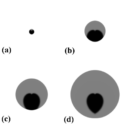
Since the two sector boundaries turn in opposite directions, they must eventually meet, thus, enclosing the less fit strain within the population of a faster growing strain, as shown in figure 13. This enclosure occurs at , and, from equation (10), we calculate the distance from the center of the inoculation to the point where the two boundaries finally meet,
| (14) |
where the last equality follows from our definition of selective advantage . Note that the time at which the second strain is enclosed by the first strain is exponentially large as . Therefore, for small , a competitive exclusion requires a much longer time than predicted by the well-mixed population models.
Equation (12) is valid only up to , and, after the enclosure, the shape of the colony is determined by the expansion of the first strain with velocity .
Another interesting consequence of the equal-time argument is that the point where the two strains meet at the colony edge moves tangentially to the front of the less fit strain with a constant velocity ; see figures 10 and 11. Indeed, the distance between the two sector boundaries at a linear front increases with time as (equation 8)
| (15) |
and the angular size of a sector in the circular geometry grows as (equation 10)
| (16) |
where the factors of 2 are due to boundary motion at both edges of a sector. The lateral expansion velocity is then given by
| (17) |
Thus, is a constant. One can also show that and these three vectors make a right triangle (); here and are front velocities at the sector boundary. Sectors of deleterious strain also obey equation (17), but with a negative lateral velocity, .
4.3 Colony collisions
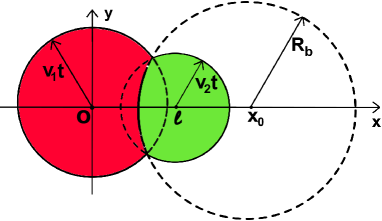
We conclude this section by considering competition between two strains not initially in contact. At the beginning of the experiment, two circular colonies inoculated with different strains grow independently each with their own velocity. Eventually, however, the colonies collide; see figure 14. For simplicity, we assume that the initial radius of the colonies is much smaller than the distance between the colonies. Provided the nutrients remain abundant by time , the colony boundaries are circles with radii and except for the collision boundary. The shape of the collision boundary follows from the equal-time argument; see figure 14. Remarkably, this boundary is also a circle, with radius given by
| (18) |
Note that diverges as the selective advantage . The center of this circle is located on the line connecting the centers of the colonies, distance away from the center of the colony established by the first (faster growing) strain. We find
| (19) |
where positive corresponds to the direction towards the colony with the second strain, and negative corresponds to the opposite direction (see figure 14). Similar to the selective sweep in the circular geometry, the less fit strain is eventually enclosed by the other strain. The time to this enclosure is given by
| (20) |
We derived sector and colony shapes using the equal-time argument and the results are consistent with our microscopic model. Because this argument relies only on the assumptions of constant expansion velocities and impenetrability of occupied regions, the equal-time argument applies more generally. As a result, we expect that the competition outcome is determined only by the ratio of expansion velocities of the two strains or species for any model consistent with these two assumptions.
5 Comparison with experiments
In the two preceding sections, we described theoretical predictions for the patterns of genetic diversity arising from spatial competitions. In section 3, we developed a generic reaction-diffusion model in order to predict macroscopic spatial patterns from microscopic parameters like cellular growth rates and effective diffusion constants. In section 4, we then derived analytical formulae for boundaries between regions occupied by the competing strains using the equal-time argument. In this section, we experimentally test our theoretical predictions, using the expansion of the budding yeast Saccharomyces cerevisiae on agar surfaces as a model system. We also employ the analytical formulae from the equal-time argument, equations (8), (10), (18), and (19), as a means to measure relative fitness of two yeast strains.
5.1 Testing the equal-time argument
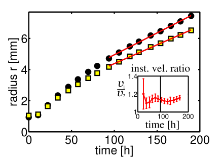
We first tested the validity of the equal-time argument results of section 4 with a particular pair of S. cerevisiae strains that have a large fitness difference: the wild-type and a faster growing mutant, which owes its advantage to the removal of a metabolically costly mating system; see the supplementary information (section S1) for more details. The equal-time argument assumes spatial expansion at a constant velocity. To see whether this assumption was valid in our experimental system, we measured the increase of the radius of circular yeast colonies over time, see figure 15. During the first day, colonies barely grow, presumably because it takes time for the populations to reach the carrying capacity in the spatial region of the inoculum. Afterwards, the colony fronts expand at about m/h. The rate of expansion first slows down gradually over time, presumably because of nutrient depletion and drying out of the agar gel. For larger times, a stationary expansion front has established, and colonies grow at a constant expansion velocity. Since the latter is a pre-requisite for the equal-time argument to apply, we only consider these later times in our further analysis. A similar behaviour was observed for the expansion of yeast colonies from a linear inoculation (data not shown), although the absolute values of the velocities were very different; e.g. for the wild-type, we obtained m/h for linear vs. m/h for circular expansions. This difference is presumably due to larger colonies and therefore more severe nutrient depletion in linear inoculations.
(a) 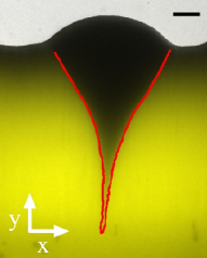 (b)
(b) 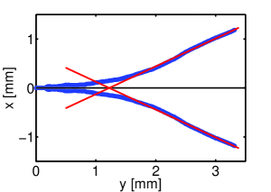
(a) 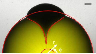 (b)
(b) 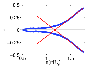
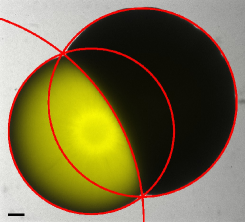 |
We next tested whether the equal-time argument correctly predicts shapes of boundaries between the strains: linear for linear expansions, logarithmic spirals for circular expansions, and circular for colliding colonies. This was indeed the case, see figures 16, 17, and 18. Note that in the case of sectors, the equal-time argument applies only at later times. During earlier times, the expansion velocity is not constant, as discussed above. In addition, during this initial transient, sectors have not yet fully established, see the discussion in section 3 and in the supplement section S5. Since both constant expansion velocity and fully established domains of each strains are required for the equal-time argument, we fit our theoretical predictions equations (8) and (10) to the sector shapes only for later times, finding excellent agreement ().
5.2 Measuring relative fitness
This agreement allows us to use the analytical results from the equal-time argument in order to measure the relative fitness . From our analysis, the relative fitness can be estimated by five different methods, using (i-ii) ratio of expansion velocities and of isolated colonies in linear and circular geometries, (iii-iv) sector shapes in linear and circular geometries using equations (8) and (10), and (v) the interface shape of colliding circular colonies using equations (18,19). For consistency, we used the same time window for all assays, see the supplementary information (section S1) for details. To provide a reference, we also measured the relative growth rate during exponential phase in a well-mixed test tube, either in separate or in mixed cultures.
| Assay | Method | Selective advantage, |
|---|---|---|
| Linear expansion | velocity ratios | |
| sectors | ||
| Radial expansion | velocity ratios | |
| sectors | ||
| colony collisions | ||
| Liquid culture | growth rate ratios | |
| competitions |
The relative fitnesses obtained from the different fitness assays yield quite similar results, summarized in table 1. Indeed, the measurements are not significantly different from each other, except for the circular sector result which differs significantly from both the liquid culture competition and the colony collision assays (, see the supplement section S6 for details on the statistical testing procedure). The deviation for circular sectors could be caused by a systematic error in sector analysis. However, a likely explanation of the disagreement between different fitness estimates is some additional spatial structure not accounted for in our theory. Indeed, yeast colonies do not only expand on the surface of a Petri dish, but they also thicken over time to a height of about mm, which is neglected in our two-dimensional theory. It is therefore possible that the advantageous mutant grows on top of the wild-type, producing an apparently larger sector and leading to an overestimate of .
Table 1 shows that the different fitness assays have standard deviations that vary over an order of magnitude, and therefore have very different accuracies. Expansion velocities of isolated single-strain colonies are the most straightforward measurement of fitness on a plate. However, they are less accurate than the sector and colony collision assays, as reflected by their high standard deviations in table 1 and the fluctuations of the instantaneous velocity ratio in the inset of figure 15. In sector and collision assays, the two competing strains are in exactly the same environment, and inevitable slight differences in the experimental conditions, such as humidity of the agar, influence both strains equally. This is not true for the isolated colonies of the expansion velocity assays, which are therefore more variable. Even more important, we found that relative fitnesses obtained from experiments on different batches of plates were significantly different when determined from expansion velocities, but not when determined from sectors or colony collisions; see the supplementary information (section S1). Nevertheless, the ratio of the expansion velocities is similar for linear and circular expansions, see table 1, despite a large difference in the absolute values of the velocities, as discussed above.
Linear expansion assays also have large standard deviations. This is probably due to undulations of linear fronts [26], clearly visible in figure 1, which distort the sector shapes. These undulations are significantly reduced in the circular geometry, leading to smaller standard deviations. It is thus advantageous to determine fitness from circular rather than linear expansions.
From this discussion and table 1, it follows that the radial expansion sector and colony collision assays are the most reliable assays to measure relative fitness in a spatial competition. We therefore only use these two spatial fitness assays in the following.
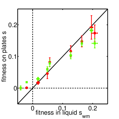 |
We have so far found agreement between experiments and our equal-time argument predictions, but only for one pair of strains with one particular fitness difference. Therefore, we performed further experiments over a range of fitness values. To this purpose, we competed a strain resistant to with a strain sensitive to cycloheximide (a drug inhibiting translation) for varying cycloheximide concentrations in the medium. The relative fitness of the resistant strain, as e.g., measured with a liquid culture competition assay, increases linearly with the drug concentration, see supplementary figure S8. For all concentrations tested, radial sectors and colony collision boundaries could be well fitted with logarithmic spirals and circles, respectively, as predicted by our theory. More importantly, we were able to compare the fitness advantage in liquid culture to the fitness advantage on Petri dishes over a wide range of relative fitnesses. We found good agreement between the two spatial assays and the liquid competition assay, see figure 19.
5.3 Testing the reaction-diffusion model
Our reaction-diffusion model predicts an agreement of the spatial and well-mixed relative fitness, if migration is driven by cell growth, i.e. and , as discussed at the end of section 3. The results shown in figure 19 are therefore a direct confirmation of this version of the reaction-diffusion model. In addition, the reaction-diffusion model predicts a constant front expansion velocity, given by equation 7, which is indeed observed in our experiments for large times, as shown in figure 15. Furthermore, the reaction-diffusion model gives rise to the same, experimentally confirmed, macroscopic spatial pattern predicted by the equal-time argument, independent of microscopic details on the cellular length scale. We therefore preformed competition experiments with S. cerevisiae strains that have different cell division patterns, as well as with the bacterium Pseudomonas aeruginosa, see supplementary information (section S3). All experiments could be well described by our theory.
In summary, there are experimental subtleties that our phenomenological theory does not take into account, such as the expansion velocity slowdown, yeast colony thickness, or possible strain interactions 444The mutualistic or antagonistic interaction represented by the terms with and in equation (4) could also change the relative fitness in experiments where the strains are in physical contact compared to experiments where the strains are grown in isolation. Three dimensional yeast colonies have a relatively large contact angle with the agar surface at the colony edge [32]. Therefore, the effect of such hypothetical interactions between the two strains might not be negligible if the density of yeast cells at the colony edge is not sufficiently small, as it would be if cell density decayed exponentially at the frontier.. All these effects could contribute to the slight differences of the fitness values determined by different methods, see table 1 and figure 19. Nevertheless, our theory describes the shapes of established sectors and colony collisions very accurately. Considering that the methods to determine relative fitness are very different, it is remarkable that the obtained fitness values are so similar, in particular results from well-mixed liquid culture and spatial growth on agar surfaces.
6 Discussion
Natural selection in well-mixed populations leads to selective sweeps of beneficial genotypes occurring exponentially fast in time. However, in spatially expanding populations, competition results in more complicated temporal and spatial patterns. Since both the advantageous and deleterious genotypes can spread into uncolonized territories, their competition can result in sectoring patterns like that shown in figure 6. Sectoring spatial patterns provide an alternative fitness assay to the commonly used assays based on competition in a well-mixed environment of a test tube. This alternative facilitates spatial evolutionary experiments, which might contribute to understanding adaptations in different environments.
The spatial assay may also be more accurate, provided front undulations, nutrient depletion, variations in agar wetness, and other experimental complications can be overcome. For small fitness differences, the assay could in principle acquire sensitivity because it measures instead of [24]. For large fitness differences, higher accuracy could also result from longer observation times, as the deleterious strain survives longer in spatial settings. A deleterious strain is eliminated linearly (linear geometry) or logarithmically (circular geometry) in time, unlike in the well-mixed environment, where it is eliminated exponentially fast. More important, a spatial competition experiment could be superior to a well-mixed one when used for screening for beneficial mutations. On a Petri dish, many beneficial mutations can be assayed in parallel from expansions started by a small fraction of fluorescently-labeled mutagenized cells mixed with wild-type cells. In addition, each mutation is spatially isolated, and a dense aggregate of cells only a few generations away from the original mutation could be easily collected for future use.
Our analysis of competition during range expansions has applications for evolutionary dynamics in spatially extended habitats as well. In particular, the predictions for one of the most important quantities in evolutionary dynamics, the duration of a selective sweep, is substantially different between spatial and nonspatial models. Deleterious genotypes persist much longer in spatial populations because the beneficial mutations spreading by Fisher waves may have to travel large distances needed, e.g., to engulf the wild-type populations, as in figure 13.
References
References
- [1] C. Darwin. On the origin of species by means of natural selection, or the preservation of favoured races in the struggle for life. New York University Press, New York, 1859.
- [2] N. H. Barton, D. E. G. Briggs, J. A. Eisen, D. B. Goldstein, and N. H. Patel. Evolution. Cold Spring Harbor Laboratory Press, Cold Spring Harbor, 2007.
- [3] S. F. Elena and R. E. Lenski. Evolution experiments with microorganisms: the dynamics and genetic bases of adaptation. Nature Reviews: Genetics, 4:457, 2003.
- [4] I. G. Ron, I. Golding, B. Lifsitz-Mercer, and E. Ben-Jacob. Bursts of sectors in expanding bacterial colonies as a possible model for tumor growth and metastases. Physica A, 320:485, 2003.
- [5] G. Lambert, L. Estvez-Salmeron, S. Oh, D. Liao, B. M. Emerson, T. D. Tlsty, and R. H. Austin. An analogy between the evolution of drug resistance in bacterial communities and malignant tissues. Nature Reviews Cancer, 11:375–382, 2011.
- [6] K. S. Korolev, M. Avlund, O. Hallatschek, and D. R. Nelson. Genetic demixing and evolution in linear stepping stone models. Reviews of Modern Physics, 82:1691–1718, 2010.
- [7] B. Kerr, C. Neuhauser, B. J. M. Bohannan, and A. M. Dean. Local migration promotes competitive restraint in a host–pathogen ’tragedy of the commons’. Nature, 442:75–78, 2006.
- [8] L. C. Coberly, W. Wei, K. Y. Sampson, J. Millstein, H. A. Wichman, and S. M. Krone. Space, Time, and Host Evolution Facilitate Coexistence of Competing Bacteriophages: Theory and Experiment. The American Naturalist, 173:121, 2009.
- [9] C. Hauert and M. Doebeli. Spatial structure often inhibits the evolution of cooperation in the snowdrift game. Nature, 428:643–646, 2004.
- [10] P. B. Rainey and M. Travisano. Adaptive radiation in a heterogeneous environment. Philosophical Transactions of the Royal Society B, 280:29–101, 1977.
- [11] J. Wakita, K. Komatsu, A. Nakahara, T. Matsuyama, and M. Matsushita. Experimental Investigation on the Validity of Population Dynamics Approach to Bacterial Colony Formation. Journal of the Physical Society of Japan, 63:1205–1211, 1994.
- [12] E. Ben-Jacob, O. Schochet, A. Tenenbaum, I. Cohen, A. Czirók, and T. Vicsek. Generic modelling of cooperative growth patterns in bacterial colonies. Nature, 368:46–49, 1994.
- [13] E. Ben-Jacob, I. Cohen, O. Shochet, I. Aranson, H. Levine, and L. Tsimring. Complex bacterial patterns. Nature, 373:566–567, 1995.
- [14] I. Golding, I. Cohen, and E. Ben-Jacob. Studies of sector formation in expanding bacterial colonies. Europhysics Letters, 48:587, 1999.
- [15] O. Hallatschek, P. Hersen, S. Ramanathan, and D. R. Nelson. Genetic drift at expanding frontiers promotes gene segregation. Proc. Natl. Acad. Sci. USA, 104:19926, 2007.
- [16] A. Be’Er, H. P. Zhang, E. L. Florin, S. M. Payne, E. Ben-Jacob, and H. L. Swinney. Deadly competition between sibling bacterial colonies. Proceedings of the National Academy of Sciences, 106:428, 2009.
- [17] K. S. Korolev, J. B. Xavier, D. R. Nelson, and K. R. Foster. A Quantitative Test of Population Genetics Using Spatio-Genetic Patterns in Bacterial Colonies. The American Naturalist, 178:538, 2011.
- [18] B. Kerr, M. A. Riley, M. W. Feldman, and B. J. M. Bohannan. Local dispersal promotes biodiversity in a real-life game of rock-paper-scissors. Nature, 418:171–174, 2002.
- [19] M. G. J. L. Habets, D. E. Rozen, R. F. Hoekstra, and J. A. G. M. de Visser. The effect of population structure on the adaptive radiation of microbial populations evolving in spatially structured environments. Ecological Letters, 9:1041–1048, 2006.
- [20] W. Harcombe. Novel cooperation experimentally evolved between species. Evolution, 64:2166–2172, 2010.
- [21] G. Saxer, M. Doebeli, and M. Travisano. Spatial structure leads to ecological breakdown and loss of diversity. Proceedings of the Royal Society B: Biological Sciences, 276:2065–2070, 2009.
- [22] G. J. Velicer and Y. T. N. Yu. Evolution of novel cooperative swarming in the bacterium myxococcus xanthus. Nature, 425:75–78, 2003.
- [23] E. Ben-Jacob, I. Cohen, and H. Levine. Cooperative self-organization of microorganisms. Advances in Physics, 49:395–554, 2000.
- [24] O. Hallatschek and D. R. Nelson. Life at the front of an expanding population. Evolution, 64:193, 2010.
- [25] O. Hallatschek. The noisy edge of traveling waves. Proceedings of the National Academy of Sciences USA, 108:1783–1787, 2011.
- [26] D. A. Kessler and H. Levine. Fluctuation-induced diffusive instabilities. Nature, 394:556, 1998.
- [27] L. Z. Pipe and M. J. Grimson. Spatial-temporal modelling of bacterial colony growth on solid media. Mol. BioSyst., 4:192–198, 2008.
- [28] C. D. Nadell, K. R. Foster, and J. B. Xavier. Emergence of spatial structure in cell groups and the evolution of cooperation. PLoS Computational Biology, 6:e1000716, 2010.
- [29] J. D. Murray. Mathematical Biology. Springer, 2003.
- [30] R. Pearl. The growth of populations. The Quarterly Review of Biology, 2:532–548, 1927.
- [31] T. Carlson. Über geschwindigkeit und grösse der hefevermehrung in würze. Biochem. Z, 57:313–334, 1913.
- [32] B. Nguyen, A. Upadhyaya, A. Van Oudenaarden, and M. P. Brenner. Elastic instability in growing yeast colonies. Biophysical Journal, 86:2740–2747, 2004.
- [33] R. A. Fisher. The wave of advance of advantageous genes. The Annals of Eugenics, 7:353, 1937.
- [34] A. N. Kolmogorov, N. Petrovsky, and N. S. Piscounov. A study of the equation of diffusion with increase in the quantity of matter, and its application to a biological problem. Moscow University Bulletin of Mathematics, 1:1, 1937.
- [35] O. Hallatschek and K. S. Korolev. Fisher Waves in the Strong Noise Limit. Physical Review Letters, 103:108103, 2009.
- [36] M. Born, E. Wolf, and A. B. Bhatia. Principles of Optics. Pergamon Press, 1964.
- [37] T. A. Cook. The Curves of Life. Dover, London, 1985.