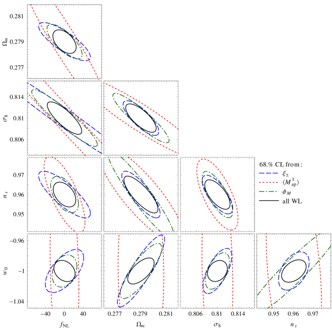
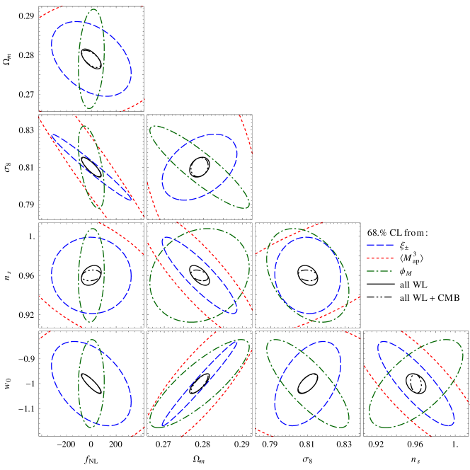
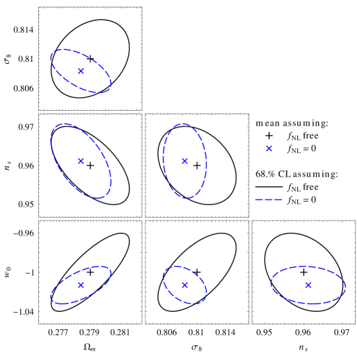
Measuring primordial non-Gaussianity with weak-lensing surveys

Stefan Hilbert1,2, Laura Marian2, Robert E. Smith2,3, and Vincent Desjacques3,4
1Kavli Institute of Particle Astrophysics and Cosmology (KIPAC), Stanford University, 452 Lomita Mall, Stanford, CA 94305, and
SLAC National Accelerator Laboratory, 2575 Sand Hill Road, M/S 29, Menlo Park, CA 94025
2Argelander-Institut für Astronomie, Auf dem Hügel 71, 53121 Bonn, Germany
3Institute for Theoretical Physics, University of Zürich, Zürich, CH 8057, Switzerland
4Universite de Geneve and Center for Astroparticle Physics, 24 Quai Ernest Ansermet, 1211 Geneve 4, Switzerland
hilbert@stanford.edu
Abstract

Measuring the non-Gaussianity of the initial matter density fluctuations may provide powerful insights into cosmic inflation and the origin of structures. Although current information on primordial non-Gaussianity comes mostly from the Cosmic Microwave Background, obtaining constraints from lower-redshift observables will be an important task for future surveys. We study the ability of future weak lensing (WL) surveys to constrain primordial non-Gaussianity of the local type. We use a large ensemble of simulated WL maps with survey specifications relevant to Euclid and LSST. The simulations assume Cold Dark Matter cosmologies that vary certain parameters around fiducial values: the non-Gaussianity parameter fNLsubscript𝑓NLf_{\text{NL}}, the matter density parameter ΩmsubscriptΩm\Omega_{\text{m}}, the amplitude of the matter power spectrum σ8subscript𝜎8\sigma_{8}, the spectral index of the primordial power spectrum nssubscript𝑛sn_{\text{s}}, and the dark-energy equation-of-state parameter w0subscript𝑤0w_{0}. We assess the sensitivity of the cosmic shear correlation functions, the third-order aperture mass statistics, and the abundance of shear peaks to these parameters. We find that each of the considered probes provides unmarginalized constraints of ΔfNL20similar-toΔsubscript𝑓NL20\Delta f_{\text{NL}}\sim 20 on fNLsubscript𝑓NLf_{\text{NL}}. Marginalized constraints from any individual WL probe are much weaker due to strong correlations between parameters. However, the parameter errors can be substantially reduced by combining information from different WL probes. Combining all WL probes yields the following marginal (68% confidence level) uncertainties: ΔfNL50similar-toΔsubscript𝑓NL50\Delta f_{\text{NL}}\sim 50, ΔΩm0.002similar-toΔsubscriptΩm0.002\Delta\Omega_{\text{m}}\sim 0.002, Δσ80.004similar-toΔsubscript𝜎80.004\Delta\sigma_{8}\sim 0.004, Δns0.007similar-toΔsubscript𝑛s0.007\Delta n_{\text{s}}\sim 0.007, and Δw00.03similar-toΔsubscript𝑤00.03\Delta w_{0}\sim 0.03. We examine the bias induced by neglecting fNLsubscript𝑓NLf_{\text{NL}} on the constraints on the other parameters. We find σ8subscript𝜎8\sigma_{8} and w0subscript𝑤0w_{0} to be the most affected. Moreover, neglecting non-Gaussianity leads to a severe underestimation of the uncertainties in the other cosmological parameters. We conclude that a full exploitation of future WL surveys requires a joint analysis of different WL probes. Furthermore, if not taken into account, a non-vanishing level of primordial non-Gaussianity will bias the estimated cosmological parameters and uncertainties for future surveys.

keywords:
gravitational lensing: weak – cosmological parameters – early Universe – inflation – large-scale structure – methods: N-body simulations

1 Introduction

According to Big Bang cosmologies, the rich matter structures seen today in our Universe have grown from tiny density fluctuations at very early times. There are a number of competing theories for the physical origins of these primordial density perturbations, e.g. the Ekpyrotic model (Khoury et al. 2001) or the string gas cosmology (Brandenberger et al. 2007). The leading explanation is the inflationary paradigm (Mukhanov and Chibisov 1981). The standard single-field slowly-rolling inflationary model provides four fundamental predictions: a nearly flat spatial curvature for spacetime, a nearly scale-invariant power spectrum of primordial curvature perturbations, a nearly Gaussian distribution of primordial density perturbations, and a scale-invariant spectrum of gravitational waves. The first three predictions have been tested by observations of the cosmic microwave background radiation (CMB) with the Wilkinson Microwave Anisotropy Probe (WMAP, Komatsu et al. 2011). The discovery of primordial gravitational wave signatures in the CMB is one of the main goals for the Planck mission (The Planck Collaboration 2006).

Recently much attention has been turned towards using observations of the statistical properties of the large-scale structure to further falsify models for the origin of density perturbations. For example, single field inflation leads to a near-Gaussian distribution of fluctuations (Acquaviva et al. 2003; Maldacena 2003). Hence, if significant departures from Gaussianity are detected, all single-field inflationary models could be ruled out (Creminelli and Zaldarriaga 2004). In such models, departures from Gaussianity can be characterized by the local expansion of the primordial potential perturbations (Matarrese et al. 2000):

Φ(𝒙)=ϕ(𝒙)+fNL[ϕ2(𝒙)ϕ2(𝒙)],Φ𝒙italic-ϕ𝒙subscript𝑓NLdelimited-[]superscriptitalic-ϕ2𝒙delimited-⟨⟩superscriptitalic-ϕ2𝒙\Phi(\boldsymbol{x})=\phi(\boldsymbol{x})+f_{\text{NL}}\left[\phi^{2}(\boldsymbol{x})-\left\langle{\phi^{2}(\boldsymbol{x})}\right\rangle\right], (1)

Here, ϕ(𝒙)italic-ϕ𝒙\phi(\boldsymbol{x}) denotes the Gaussian potential perturbation at spacetime point 𝒙𝒙\boldsymbol{x} after matter radiation equality, and the parameter fNLsubscript𝑓NLf_{\text{NL}} quantifies the deviation from Gaussianity. In linear theory, typical fluctuations are very small with ϕ105similar-toitalic-ϕsuperscript105\phi\sim 10^{-5}. Thus, for |fNL|<105subscript𝑓NLsuperscript105|f_{\text{NL}}|<10^{5}, the typical non-Gaussian corrections, are small, too: (Φϕ)/ϕfNLϕsimilar-toΦitalic-ϕitalic-ϕsubscript𝑓NLitalic-ϕ(\Phi-\phi)/\phi\sim f_{\text{NL}}\phi.

Currently, the best constraints on local-type primordial non-Gaussianity come from the CMB bispectrum in the seven-year WMAP data (Komatsu et al. 2011): fNL=32±21subscript𝑓NLplus-or-minus3221f_{\text{NL}}=32\pm 21 at 68% confidence level (CL). Though not widely anticipated a few years ago, it has recently been shown that probes of structures at lower redshifts could also provide competitive constraints, in particular the nonlinear matter power spectrum (Seto 2001; Amara and Refregier 2004; Desjacques et al. 2009; Pillepich et al. 2010; Smith et al. 2011), the abundance of massive clusters (Matarrese et al. 2000; Lo Verde et al. 2008), the galaxy bispectrum (Sefusatti and Komatsu 2007; Nishimichi et al. 2010; Baldauf et al. 2011; Sefusatti et al. 2012), and the scale-dependence of galaxy clustering (Dalal et al. 2008; Desjacques et al. 2009; Pillepich et al. 2010).

In this paper, we focus on the question: How well can a large weak lensing (WL) survey constrain the level of primordial non-Gaussianity in the initial conditions? This is of prime concern given upcoming surveys like the Kilo Degree Survey (KiDS, 1500deg2similar-toabsent1500superscriptdeg2\sim 1500\,\mathrm{deg}^{2}, Kuijken 2007) and the Dark Energy Survey (DES, 5500deg2similar-toabsent5500superscriptdeg2\sim 5500\,\mathrm{deg}^{2}, The Dark Energy Survey Collaboration 2005), or planned full sky surveys such as those with Euclid (15 000deg2similar-toabsent15000superscriptdeg2\sim 15\,000\,\mathrm{deg}^{2}, Laureijs et al. 2011) or the Large Synoptic Survey Telescope (LSST,20 000deg2similar-toabsent20000superscriptdeg2\sim 20\,000\,\mathrm{deg}^{2}, LSST Science Collaborations and LSST Project 2009).

There have been various forecasts for the expected error ΔfNLΔsubscript𝑓NL\Delta f_{\text{NL}} on the non-Gaussianity parameter fNLsubscript𝑓NLf_{\text{NL}} from future weak lensing surveys. For example, Jeong et al. (2009) predicted that ΔfNL50Δsubscript𝑓NL50\Delta f_{\text{NL}}\approx 50 could be obtained from galaxy-galaxy lensing on large angular scales. Fedeli and Moscardini (2010) found that ΔfNL<Δsubscript𝑓NLabsent\Delta f_{\text{NL}}< a few tens may be possible from a χ2superscript𝜒2\chi^{2}-analysis of the convergence power spectrum. Using a halo model, Maturi et al. (2011) obtained ΔfNL30similar-toΔsubscript𝑓NL30\Delta f_{\text{NL}}\sim 30 for a combined analysis of the convergence power spectra and the abundance of shear peaks in a Euclid-like survey. Schäfer et al. (2012) predicted that ΔfNL200Δsubscript𝑓NL200\Delta f_{\text{NL}}\approx 200 could be achieved from analyzing convergence bispectra, which could be further reduced to ΔfNL30Δsubscript𝑓NL30\Delta f_{\text{NL}}\approx 30 if sufficiently tight priors on all other relevant cosmological parameters are available. Giannantonio et al. (2012) found that a combined analysis of weak lensing and galaxy clustering could give ΔfNL<10Δsubscript𝑓NL10\Delta f_{\text{NL}}<10. Oguri and Takada (2011) estimated ΔfNL10similar-toΔsubscript𝑓NL10\Delta f_{\text{NL}}\sim 10 for an imaging survey combining cluster counts, the cluster correlation function, and stacked WL signals of clusters.

Whilst this is encouraging, all these studies rely heavily upon approximations for the nonlinear matter power spectrum, bispectrum and analytic modelling of shear peak abundances that are not well tested or understood in non-Gaussian models. Furthermore, the gain in information from combining different probes has not yet been fully investigated. Instead, approximations of various degrees of plausibility have been made for the cross-covariances between different observables. Moreover, most of these forecasts ignore degeneracies of fNLsubscript𝑓NLf_{\text{NL}} with other cosmological parameters. Thus, one should be circumspect when interpreting these forecasts.

In this paper we take a more direct approach to answering this question. We use an ensemble of N𝑁N-body simulations of structure formation in flat Dark-Energy Cold-Dark-Matter (w𝑤wCDM) cosmologies, through which we perform full gravitational ray-tracing to construct a suite of large mock weak lensing maps (e.g. the maps for our fiducial cosmological model cover a total area of 14 000deg214000superscriptdeg214\,000\,\mathrm{deg}^{2}). Initial results from these simulations were already presented in Marian et al. (2011), where we showed that the abundance of shear peaks was sensitive to fNLsubscript𝑓NLf_{\text{NL}}, and that one may obtain an error of ΔfNL13Δsubscript𝑓NL13\Delta f_{\text{NL}}\approx 13 when all other cosmological parameters are known. In this work we present a much wider study about combining information from the cosmic-shear two-point correlations ξ+subscript𝜉\xi_{+} and ξsubscript𝜉\xi_{-}, the aperture mass statistics Map3delimited-⟨⟩superscriptsubscript𝑀ap3\bigl{\langle}{M_{\text{ap}}^{3}}\bigr{\rangle}, and the abundance of shear peaks ϕMsubscriptitalic-ϕ𝑀\phi_{M}. Our approach allows us to fully explore the cross-correlations between these different weak lensing probes. Furthermore, the initial suite of simulations used in Marian et al. (2011) are augmented with cosmological models that take into account variations in other cosmological parameters. Thus, we can investigate the joint constraints from WL in the parameter space spanned by: the non-Gaussianity parameter fNLsubscript𝑓NLf_{\text{NL}}, the mean matter density ΩmsubscriptΩm\Omega_{\text{m}}, normalization σ8subscript𝜎8\sigma_{8} and spectral index nssubscript𝑛sn_{\text{s}} of the matter power spectrum, and the equation-of-state (EOS) parameter w0subscript𝑤0w_{0} of the dark energy (DE).

Ray-tracing simulations have been used recently by Pace et al. (2011) and Fedeli et al. (2011) to study the effects of primordial non-Gaussianity on basic lensing quantities and the skeleton of the convergence field. In contrast to their work, we focus in our work on observables more easily accessible in weak lensing surveys. Moreover, we include realistic levels of noise directly in our simulations for the error analysis. Finally, our larger set of simulations allows us to explore a higher-dimensional parameter space in a uniform manner.

The paper is broken down as follows: In Section 2, we briefly discuss the weak lensing cosmological probes that we employ in this study. In Section 3, we give an overview of the cosmological N𝑁N-body simulations and the ray-tracing, and review how we estimate the observables and their covariance from the simulated data. In Section 4, we consider the effects of primordial non-Gaussianity on the weak lensing observables. We also discuss the expected statistical uncertainties and covariances of the weak lensing observables as well as their dependence on the full set of considered cosmological parameters. Furthermore, we present forecasts for unmarginalized and marginalized constraints on cosmological parameters, and discuss possible biases arising from neglecting finite non-Gaussianity. The paper concludes with a summary and discussion in Section 5.

2 Theory

2.1 Gravitational lensing

Gravitational lensing is the process whereby photon bundles emitted from distant light sources are deflected by the gravitational field of matter structures along the line of sight. These deflections can thus magnify, shift and shear the images of distant galaxies (e.g. Bartelmann and Schneider 2001; Schneider et al. 2006). The observed image position 𝜽=(θ1,θ2)𝜽subscript𝜃1subscript𝜃2\boldsymbol{\theta}=(\theta_{1},\theta_{2}) of a source at redshift z𝑧z may thus differ from the source’s ‘true’ angular position 𝜷=(β1(𝜽,z),β2(𝜽,z))𝜷subscript𝛽1𝜽𝑧subscript𝛽2𝜽𝑧\boldsymbol{\beta}=\bigl{(}\beta_{1}(\boldsymbol{\theta},z),\beta_{2}(\boldsymbol{\theta},z)\bigr{)}. Image distortions caused by differential deflection can be quantified locally by the distortion matrix

(βi(𝜽,z)θj)i,j=1,2=(1κγ1γ2ωγ2+ω1κ+γ1),subscriptsubscript𝛽𝑖𝜽𝑧subscript𝜃𝑗formulae-sequence𝑖𝑗12matrix1𝜅subscript𝛾1subscript𝛾2𝜔subscript𝛾2𝜔1𝜅subscript𝛾1\left(\frac{\partial{\beta_{i}(\boldsymbol{\theta},z)}}{\partial{\theta_{j}}}\right)_{i,j=1,2}=\begin{pmatrix}1-\kappa-\gamma_{1}&-\gamma_{2}-\omega\\ -\gamma_{2}+\omega&1-\kappa+\gamma_{1}\end{pmatrix}, (2)

whose decomposition defines the convergence κ(𝜽,z)𝜅𝜽𝑧\kappa(\boldsymbol{\theta},z), the complex shear γ(𝜽,z)=γ1(𝜽,z)+iγ2(𝜽,z)𝛾𝜽𝑧subscript𝛾1𝜽𝑧isubscript𝛾2𝜽𝑧\gamma(\boldsymbol{\theta},z)=\gamma_{1}(\boldsymbol{\theta},z)+\mathrm{i}\gamma_{2}(\boldsymbol{\theta},z), and the asymmetry ω(𝜽,z)𝜔𝜽𝑧\omega(\boldsymbol{\theta},z). In weak lensing, the asymmetry ω𝜔\omega is usually small enough to be neglected (e.g. Hilbert et al. 2009; Krause and Hirata 2010). In that case, the convergence κ𝜅\kappa and shear γ𝛾\gamma are related by a simple phase factor in Fourier space. Thus, in weak lensing, the shear field contains the same information as the convergence.

To a good approximation, the convergence is given by a projection of the matter density along the line of sight weighted by a geometrical factor, which depends on the distances between observer, deflecting matter structure, and source. The convergence field thus bears information on the growth of structures as well as on the large-scale geometry of the Universe.

For a population of sources with known redshift distribution pz(z)subscript𝑝𝑧𝑧p_{z}(z), an effective convergence and shear can be defined by

κ(𝜽)𝜅𝜽\displaystyle\kappa(\boldsymbol{\theta}) =dzpz(z)κ(𝜽,z)andabsentdifferential-d𝑧subscript𝑝𝑧𝑧𝜅𝜽𝑧and\displaystyle=\int\!\!\mathrm{d}{z}\,p_{z}(z)\kappa(\boldsymbol{\theta},z)\quad\text{and} (3)
γ(𝜽)𝛾𝜽\displaystyle\gamma(\boldsymbol{\theta}) =dzpz(z)γ(𝜽,z).absentdifferential-d𝑧subscript𝑝𝑧𝑧𝛾𝜽𝑧\displaystyle=\int\!\!\mathrm{d}{z}\,p_{z}(z)\gamma(\boldsymbol{\theta},z). (4)

Furthermore, the shear γ(𝜽)𝛾𝜽\gamma(\boldsymbol{\theta}) at a position 𝜽𝜽\boldsymbol{\theta} can be decomposed into a tangential component γt(𝜽,ϑ)subscript𝛾t𝜽bold-italic-ϑ\gamma_{\mathrm{t}}(\boldsymbol{\theta},\boldsymbol{\vartheta}) and a cross component γ×(𝜽,ϑ)subscript𝛾𝜽bold-italic-ϑ\gamma_{\times}(\boldsymbol{\theta},\boldsymbol{\vartheta}) with respect to any given direction ϑbold-italic-ϑ\boldsymbol{\vartheta} (e.g. Schneider et al. 2002b):

γt(𝜽,ϑ)subscript𝛾t𝜽bold-italic-ϑ\displaystyle\gamma_{\mathrm{t}}(\boldsymbol{\theta},\boldsymbol{\vartheta}) =[γ(𝜽)e2iφ(ϑ)]andabsent𝛾𝜽superscripte2i𝜑bold-italic-ϑand\displaystyle=-\Re\!\left[\!\gamma(\boldsymbol{\theta})\mathrm{e}^{-2\mathrm{i}\varphi(\boldsymbol{\vartheta})}\!\right]\quad\text{and} (5)
γ×(𝜽,ϑ)subscript𝛾𝜽bold-italic-ϑ\displaystyle\gamma_{\times}(\boldsymbol{\theta},\boldsymbol{\vartheta}) =[γ(𝜽)e2iφ(ϑ)],absent𝛾𝜽superscripte2i𝜑bold-italic-ϑ\displaystyle=-\Im\!\left[\!\gamma(\boldsymbol{\theta})\mathrm{e}^{-2\mathrm{i}\varphi(\boldsymbol{\vartheta})}\!\right], (6)

where φ(ϑ)𝜑bold-italic-ϑ\varphi(\boldsymbol{\vartheta}) denotes the polar angle of the vector ϑbold-italic-ϑ\boldsymbol{\vartheta}.

2.2 Weak lensing observables

Owing to the fact that we do not know the intrinsic shapes of individual background galaxies, the quantities κ𝜅\kappa and γ𝛾\gamma are not direct observables. Nevertheless, we can use correlations in the shapes of the background galaxies to construct quantities that are observable.

2.2.1 Cosmic shear correlation functions

In this study, the first set of lensing observables that we consider are the cosmic shear two-point correlation functions (e.g. Kaiser 1992):

ξ±(|ϑ|)subscript𝜉plus-or-minusbold-italic-ϑ\displaystyle\xi_{\pm}\bigl{(}\lvert\boldsymbol{\vartheta}\rvert\bigr{)} =γt(𝜽,ϑ)γt(𝜽+ϑ,ϑ)±γ×(𝜽,ϑ)γ×(𝜽+ϑ,ϑ),absentplus-or-minusdelimited-⟨⟩subscript𝛾t𝜽bold-italic-ϑsubscript𝛾t𝜽bold-italic-ϑbold-italic-ϑdelimited-⟨⟩subscript𝛾𝜽bold-italic-ϑsubscript𝛾𝜽bold-italic-ϑbold-italic-ϑ\displaystyle=\left\langle{\gamma_{\mathrm{t}}(\boldsymbol{\theta},\boldsymbol{\vartheta})\gamma_{\mathrm{t}}(\boldsymbol{\theta}+\boldsymbol{\vartheta},\boldsymbol{\vartheta})}\right\rangle\pm\left\langle{\gamma_{\times}(\boldsymbol{\theta},\boldsymbol{\vartheta})\gamma_{\times}(\boldsymbol{\theta}+\boldsymbol{\vartheta},\boldsymbol{\vartheta})}\right\rangle, (7)

where the angle brackets delimited-⟨⟩\bigl{\langle}{\dots}\bigr{\rangle} denote the expectation for an ensemble of universes constrained to have a particular set of cosmological parameters. The cosmic shear correlation functions ξ+subscript𝜉\xi_{+} and ξsubscript𝜉\xi_{-} can be directly estimated from the observed ellipticities of the images of distant galaxies.

In weak lensing, the shear correlation functions can be written in terms of the convergence power spectrum (Kaiser 1992):

ξ+/(ϑ)=0d2πJ0/4(ϑ)Pκ(),subscript𝜉absentitalic-ϑsuperscriptsubscript0d2𝜋subscript𝐽04italic-ϑsubscript𝑃𝜅\xi_{+/-}(\vartheta)=\int_{0}^{\infty}\frac{\mathrm{d}\ell\ell}{2\pi}J_{0/4}(\ell\vartheta)P_{\kappa}(\ell), (8)

where Jn(x)subscript𝐽𝑛𝑥J_{n}(x) denotes the Bessel function of the first kind, and Pκ()subscript𝑃𝜅P_{\kappa}(\ell) denotes the angular power spectrum of convergence fluctuations.

2.2.2 Aperture mass statistics

The aperture mass Map(𝜽,ϑ)subscript𝑀ap𝜽italic-ϑM_{\text{ap}}(\boldsymbol{\theta},\vartheta) at position 𝜽𝜽\boldsymbol{\theta} and scale ϑitalic-ϑ\vartheta can be defined as a filtered version of convergence or shear field (Schneider et al. 1998):

Map(𝜽,ϑ)=d2𝜽U(|𝜽𝜽|,ϑ)κ(𝜽)=d2𝜽Q(|𝜽𝜽|,ϑ)γt(𝜽,𝜽𝜽),=[d2𝜽Q(|𝜽𝜽|,ϑ)e2iφ(𝜽𝜽)γ(𝜽)]\begin{split}M_{\text{ap}}(\boldsymbol{\theta},\vartheta)&=\int\mathrm{d}^{2}{\boldsymbol{\theta}^{\prime}}U(\lvert\boldsymbol{\theta}^{\prime}-\boldsymbol{\theta}\rvert,\vartheta)\kappa(\boldsymbol{\theta}^{\prime})\\ &=\int\mathrm{d}^{2}{\boldsymbol{\theta}^{\prime}}Q(\lvert\boldsymbol{\theta}^{\prime}-\boldsymbol{\theta}\rvert,\vartheta)\gamma_{\mathrm{t}}(\boldsymbol{\theta}^{\prime},\boldsymbol{\theta}^{\prime}-\boldsymbol{\theta}),\\ &=-\Re\left[\int\mathrm{d}^{2}{\boldsymbol{\theta}^{\prime}}Q(\lvert\boldsymbol{\theta}^{\prime}-\boldsymbol{\theta}\rvert,\vartheta)\mathrm{e}^{-2\mathrm{i}\varphi(\boldsymbol{\theta}^{\prime}-\boldsymbol{\theta})}\gamma(\boldsymbol{\theta}^{\prime})\right]\end{split} (9)

where

Q(θ,ϑ)=2θ20θdθθU(θ,ϑ)U(θ,ϑ).𝑄𝜃italic-ϑ2superscript𝜃2superscriptsubscript0𝜃differential-dsuperscript𝜃superscript𝜃𝑈superscript𝜃italic-ϑ𝑈𝜃italic-ϑQ(\theta,\vartheta)=\frac{2}{\theta^{2}}\int_{0}^{\theta}\mathrm{d}{\theta^{\prime}}\theta^{\prime}U(\theta^{\prime},\vartheta)-U(\theta,\vartheta). (10)

Here, we use the third-order aperture mass statistics Map3(ϑ)=Map(𝜽,ϑ)3delimited-⟨⟩superscriptsubscript𝑀ap3italic-ϑdelimited-⟨⟩subscript𝑀apsuperscript𝜽italic-ϑ3\bigl{\langle}{M_{\text{ap}}^{3}}\bigr{\rangle}(\vartheta)=\bigl{\langle}{M_{\text{ap}}(\boldsymbol{\theta},\vartheta)^{3}}\bigr{\rangle} with the filter functions

U(θ,ϑ)𝑈𝜃italic-ϑ\displaystyle U(\theta,\vartheta) =12πϑ2(1θ22ϑ2)exp(θ22ϑ2)absent12𝜋superscriptitalic-ϑ21superscript𝜃22superscriptitalic-ϑ2superscript𝜃22superscriptitalic-ϑ2\displaystyle=\frac{1}{2\pi\vartheta^{2}}\left(1-\frac{\theta^{2}}{2\vartheta^{2}}\right)\exp\left(\frac{-\theta^{2}}{2\vartheta^{2}}\right)\quad\Leftrightarrow (11a)
Q(θ,ϑ)𝑄𝜃italic-ϑ\displaystyle Q(\theta,\vartheta) =θ24πϑ4exp(θ22ϑ2)absentsuperscript𝜃24𝜋superscriptitalic-ϑ4superscript𝜃22superscriptitalic-ϑ2\displaystyle=\frac{\theta^{2}}{4\pi\vartheta^{4}}\exp\left(\frac{-\theta^{2}}{2\vartheta^{2}}\right) (11b)

as another lensing probe of cosmology. The statistics Map3(ϑ)delimited-⟨⟩superscriptsubscript𝑀ap3italic-ϑ\bigl{\langle}{M_{\text{ap}}^{3}}\bigr{\rangle}(\vartheta) can also be estimated in a straightforward manner from the observed image ellipticities of distant galaxies (Schneider et al. 1998).

In the limit of weak lensing, the expectation value of Map3superscriptsubscript𝑀ap3M_{\text{ap}}^{3} is related to the convergence bispectrum Bκsubscript𝐵𝜅B_{\kappa} by (e.g. Schneider et al. 2005):

Map3(ϑ)=24π0d/2d0arccos(2)dφ×U~(,ϑ)U~(,ϑ)U~(′′,ϑ)Bκ(,,′′),delimited-⟨⟩superscriptsubscript𝑀ap3italic-ϑ24𝜋superscriptsubscript0differential-dsuperscriptsubscript2differential-dsuperscriptsuperscriptsuperscriptsubscript02superscriptdifferential-d𝜑~𝑈italic-ϑ~𝑈superscriptitalic-ϑ~𝑈superscript′′italic-ϑsubscript𝐵𝜅superscriptsuperscript′′\begin{split}\bigl{\langle}{M_{\text{ap}}^{3}}\bigr{\rangle}(\vartheta)&=24\pi\!\!\int_{0}^{\infty}\!\!\mathrm{d}\ell\ell\!\!\int_{\ell/2}^{\ell}\!\!\mathrm{d}\ell^{\prime}\ell^{\prime}\!\!\int_{0}^{\arccos\left(\frac{\ell}{2\ell^{\prime}}\right)}\!\!\mathrm{d}\varphi\\ &\quad\times\tilde{U}(\ell,\vartheta)\tilde{U}(\ell^{\prime},\vartheta)\tilde{U}(\ell^{\prime\prime},\vartheta)B_{\kappa}(\ell,\ell^{\prime},\ell^{\prime\prime}),\end{split} (12)

where ′′=2+22cosφsuperscript′′superscript2superscript22superscript𝜑\ell^{\prime\prime}=\sqrt{\ell^{2}+\ell^{\prime 2}-2\ell\ell^{\prime}\cos\varphi}, and U~(,ϑ)~𝑈italic-ϑ\tilde{U}(\ell,\vartheta) denotes the (two-dimensional) Fourier transform of the filter U(θ,ϑ)𝑈𝜃italic-ϑU(\theta,\vartheta).

2.2.3 Shear peak abundance

The observed shear field can be used to search for massive galaxy groups and clusters by applying a filter function matched to their expected lensing signal (e.g. Hamana et al. 2004). Here, we consider the hierarchical filtering method (Marian et al. 2009, 2011, 2012) with aperture-mass filters following the expected lensing signal of the Navarro-Frenk-White (NFW) profiles (Navarro et al. 1997). The observed shear field is convolved with a series of filters Qm(𝜽;M)subscript𝑄m𝜽𝑀Q_{\text{m}}(\boldsymbol{\theta};M) of different size, from the largest down to the smallest. The size is parametrized by the filter mass M𝑀M:

Qm(𝜽;M)=𝒞(M)γm(𝜽;M),subscript𝑄m𝜽𝑀𝒞𝑀subscript𝛾m𝜽𝑀Q_{\text{m}}(\boldsymbol{\theta};M)=\mathcal{C}(M)\gamma_{\text{m}}(\boldsymbol{\theta};M), (13)

where γm(𝜽;M)subscript𝛾m𝜽𝑀\gamma_{\text{m}}(\boldsymbol{\theta};M) is the shear signal expected for an NFW halo of virial mass M𝑀M at a model redshift zm=0.3subscript𝑧m0.3z_{\text{m}}=0.3 (which is roughly where halos are most effective lenses for the considered source redshifts). These weights (approximately) maximize the signal-to-noise ratio for the corresponding peaks (Marian et al. 2009, 2011). The normalization 𝒞(M)𝒞𝑀\mathcal{C}(M) is chosen such that the expected filtered signal of a halo of mass M𝑀M at the model redshift zmsubscript𝑧mz_{\text{m}} equals the halo mass M𝑀M.

All maxima in the filtered shear maps are considered as potential shear peaks. Several selection criteria are used to decide whether to regard a maximum indeed as shear peak: i) The maximum must have a signal-to-noise ratio larger than a particular threshold. ii) Its amplitude Mapsubscript𝑀apM_{\text{ap}} must be equal or larger than the mass of the filter M𝑀M used in the smoothing. iii) Its position must have a certain minimum separation to other peaks with larger amplitude.

A peak will appear with different amplitudes in maps smoothed with filters of different size. To assign a unique peak amplitude to a peak at position 𝜽𝜽\boldsymbol{\theta}, we seek the filter mass M𝑀M that matches the peak amplitude Map(𝜽;M)subscript𝑀ap𝜽𝑀M_{\text{ap}}(\boldsymbol{\theta};M), i.e. we solve the equation Map(𝜽;M)=Msubscript𝑀ap𝜽𝑀𝑀M_{\text{ap}}(\boldsymbol{\theta};M)=M for M𝑀M (see Marian et al. 2012, for details). This removes the arbitrariness in the choice of filter scale. Moreover, the resulting filter size also maximizes the signal-to-noise ratio S/N𝑆𝑁S/N for an NFW halo of virial mass M𝑀M at the model redshift zm=0.3subscript𝑧m0.3z_{\text{m}}=0.3 thanks to our particular definition of the filter amplitude. This should also (roughly) maximize the sensitivity of the shear peak counts to peaks caused by real structures, and thereby to cosmological parameters. In the rest of this text, when we refer to the ‘mass’ of a peak, we shall mean the filter mass M𝑀M for which equation Map=Msubscript𝑀ap𝑀M_{\text{ap}}=M is satisfied.

The number of observed peaks in the filtered fields contains information on the abundance of massive structures, and thus on the cosmology (e.g. Marian and Bernstein 2006; Dietrich and Hartlap 2010). We define the differential peak abundance ϕM(M)subscriptitalic-ϕ𝑀𝑀\phi_{M}(M) at filter mass M𝑀M is by:

ϕM(M)=NM(M,A)Alog10(M),subscriptitalic-ϕ𝑀𝑀subscript𝑁𝑀𝑀𝐴𝐴subscript10𝑀\begin{split}\phi_{M}(M)=-\frac{\partial N_{M}(M,A)}{A\;\partial\log_{10}(M)},\end{split} (14)

where NM(M,A)subscript𝑁𝑀𝑀𝐴N_{M}(M,A) is the number of peaks with peak mass Mabsent𝑀\geq M in the survey area A𝐴A. This shear peak abundance serves as our third cosmological probe.

In a weak-lensing survey, shear peaks can be readily identified and their amplitudes estimated using the observed image ellipticities of galaxies (see, e.g., Miyazaki et al. 2002, for an early work). Unfortunately, to date, there is no satisfactory method to predict the abundance of shear peaks for a given cosmology and survey design other than numerical simulations of lensing, which we employ here.

2.3 Estimation of cosmological parameters

We discuss the ability of future weak lensing surveys to constrain cosmological parameters within a Bayesian framework. We consider a collection of model universes {(𝝅)}𝝅\{\mathcal{M}(\boldsymbol{\pi})\} characterized by a set of Npsubscript𝑁pN_{\text{p}} cosmological parameters 𝝅=(π1,,πNp)𝗍𝝅superscriptsubscript𝜋1subscript𝜋subscript𝑁p𝗍\boldsymbol{\pi}=(\pi_{1},\ldots,\pi_{N_{\text{p}}})^{\mathsf{t}}, together with a set {𝒅}𝒅\{\boldsymbol{d}\} of Ndsubscript𝑁dN_{\text{d}}-dimensional vectors 𝒅=(d1,,dNd)𝗍𝒅superscriptsubscript𝑑1subscript𝑑subscript𝑁d𝗍\boldsymbol{d}=(d_{1},\ldots,d_{N_{\text{d}}})^{\mathsf{t}} of observational data taken in order to constrain the parameters 𝝅𝝅\boldsymbol{\pi}. The knowledge about the probability of having the model universe with parameters 𝝅𝝅\boldsymbol{\pi} realized regardless of the outcome of the observations is assumed to be quantified by a prior probability p(𝝅)𝑝𝝅p(\boldsymbol{\pi}). We also assume that we know the probability that the observations yield the data 𝒅𝒅\boldsymbol{d}, given that the underlying model \mathcal{M} has parameters 𝝅𝝅\boldsymbol{\pi}. This probability is denoted L(𝝅|𝒅)=p(𝒅|𝝅)𝐿conditional𝝅𝒅𝑝conditional𝒅𝝅L(\boldsymbol{\pi}|\boldsymbol{d})=p(\boldsymbol{d}|\boldsymbol{\pi}), and referred to as the likelihood. The posterior probability p(𝝅|𝒅)𝑝conditional𝝅𝒅p(\boldsymbol{\pi}|\boldsymbol{d}), i.e. the probability of having the parameters 𝝅𝝅\boldsymbol{\pi} realized in case the observations have yielded the data 𝒅𝒅\boldsymbol{d}, can then be computed by:

p(𝝅|𝒅)=L(𝝅|𝒅)p(𝝅)dNp𝝅L(𝝅|𝒅)p(𝝅).𝑝conditional𝝅𝒅𝐿conditional𝝅𝒅𝑝𝝅superscriptdsubscript𝑁psuperscript𝝅𝐿conditionalsuperscript𝝅𝒅𝑝superscript𝝅p(\boldsymbol{\pi}|\boldsymbol{d})=\frac{L(\boldsymbol{\pi}|\boldsymbol{d})p(\boldsymbol{\pi})}{\int\mathrm{d}^{N_{\text{p}}}{\boldsymbol{\pi}^{\prime}}\,L(\boldsymbol{\pi}^{\prime}|\boldsymbol{d})p(\boldsymbol{\pi}^{\prime})}. (15)

2.3.1 The likelihood

For simplicity, we approximate all relevant probabilities by piecewise constant or multivariate normal distributions. We assume a simple multivariate normal likelihood

L(𝝅|𝒅)=|𝗖d1|1/2(2π)Nd/2exp{12[𝒅𝝁(𝝅)]𝗍𝗖d1[𝒅𝝁(𝝅)]},𝐿conditional𝝅𝒅superscriptsuperscriptsubscript𝗖d112superscript2𝜋subscript𝑁d212superscriptdelimited-[]𝒅𝝁𝝅𝗍superscriptsubscript𝗖d1delimited-[]𝒅𝝁𝝅L(\boldsymbol{\pi}|\boldsymbol{d})=\frac{\left\lvert\boldsymbol{\mathsf{C}}_{\text{d}}^{-1}\right\rvert^{1/2}}{(2\pi)^{N_{\text{d}}/2}}\exp\left\{-\frac{1}{2}\left[\boldsymbol{d}-\boldsymbol{\mu}(\boldsymbol{\pi})\right]^{\mathsf{t}}\boldsymbol{\mathsf{C}}_{\text{d}}^{-1}\left[\boldsymbol{d}-\boldsymbol{\mu}(\boldsymbol{\pi})\right]\right\}, (16)

where the mean is given by a model prediction 𝝁(𝝅)𝝁𝝅\boldsymbol{\mu}(\boldsymbol{\pi}), and the covariance matrix 𝗖dsubscript𝗖d\boldsymbol{\mathsf{C}}_{\text{d}} is assumed model-independent. From a large set of Nrsubscript𝑁rN_{\text{r}} (Nr1much-greater-thansubscript𝑁r1N_{\text{r}}\gg 1) independent realizations 𝒅rsubscript𝒅𝑟\boldsymbol{d}_{r} of the data vector for a model with parameters 𝝅𝝅\boldsymbol{\pi}, one can estimate the model prediction 𝝁𝝁\boldsymbol{\mu} by the sample mean 𝝁^^𝝁\hat{\boldsymbol{\mu}},

𝝁(𝝅)𝝁^=1Nrr=1Nr𝒅r,𝝁𝝅^𝝁1subscript𝑁rsuperscriptsubscript𝑟1subscript𝑁rsubscript𝒅𝑟\boldsymbol{\mu}(\boldsymbol{\pi})\approx\hat{\boldsymbol{\mu}}=\frac{1}{N_{\text{r}}}\sum_{r=1}^{N_{\text{r}}}\boldsymbol{d}_{r}, (17)

and the data covariance 𝗖dsubscript𝗖d\boldsymbol{\mathsf{C}}_{\text{d}} by the sample covariance 𝗖^dsubscript^𝗖d\hat{\boldsymbol{\mathsf{C}}}_{\text{d}},

𝗖d𝗖^d=1Nr1r=1Nr[𝒅r𝝁(𝝅)][𝒅r𝝁(𝝅)]𝗍.subscript𝗖dsubscript^𝗖d1subscript𝑁r1superscriptsubscript𝑟1subscript𝑁rdelimited-[]subscript𝒅𝑟𝝁𝝅superscriptdelimited-[]subscript𝒅𝑟𝝁𝝅𝗍\boldsymbol{\mathsf{C}}_{\text{d}}\approx\hat{\boldsymbol{\mathsf{C}}}_{\text{d}}=\frac{1}{N_{\text{r}}-1}\sum_{r=1}^{N_{\text{r}}}\bigl{[}\boldsymbol{d}_{r}-\boldsymbol{\mu}(\boldsymbol{\pi})\bigr{]}\bigl{[}\boldsymbol{d}_{r}-\boldsymbol{\mu}(\boldsymbol{\pi})\bigr{]}^{\mathsf{t}}. (18)

For normal distributions, the inverse covariance 𝗖d1superscriptsubscript𝗖d1\boldsymbol{\mathsf{C}}_{\text{d}}^{-1} is best estimated by (Anderson 2003; Hartlap et al. 2007):

𝗖d1NrNd2Nr1(𝗖^d)1,superscriptsubscript𝗖d1subscript𝑁rsubscript𝑁d2subscript𝑁r1superscriptsubscript^𝗖d1\boldsymbol{\mathsf{C}}_{\text{d}}^{-1}\approx\frac{N_{\text{r}}-N_{\text{d}}-2}{N_{\text{r}}-1}\bigl{(}\hat{\boldsymbol{\mathsf{C}}}_{\text{d}}\bigr{)}^{-1}, (19)

which requires Nr>Nd+2subscript𝑁rsubscript𝑁d2N_{\text{r}}>N_{\text{d}}+2 realizations.

The maximum-likelihood parameter set 𝝅ml(𝒅)subscript𝝅ml𝒅\boldsymbol{\pi}_{\text{ml}}(\boldsymbol{d}) for the measured data 𝒅𝒅\boldsymbol{d} is given by the equation

𝟎=𝝁(𝝅)𝝅|𝝅ml𝗍𝗖d1[𝒅𝝁(𝝅ml)].0evaluated-at𝝁𝝅𝝅subscript𝝅ml𝗍superscriptsubscript𝗖d1delimited-[]𝒅𝝁subscript𝝅ml\boldsymbol{0}=\left.\frac{\partial{\boldsymbol{\mu}(\boldsymbol{\pi})}}{\partial{\boldsymbol{\pi}}}\right|_{\boldsymbol{\pi}_{\text{ml}}}^{\mathsf{t}}\boldsymbol{\mathsf{C}}_{\text{d}}^{-1}\left[\boldsymbol{d}-\boldsymbol{\mu}(\boldsymbol{\pi}_{\text{ml}})\right]. (20)

A Taylor expansion of the log-likelihood lnL(𝝅|𝒅)𝐿conditional𝝅𝒅\ln L(\boldsymbol{\pi}|\boldsymbol{d}) around the maximum-likelihood parameters 𝝅mlsubscript𝝅ml\boldsymbol{\pi}_{\text{ml}} up to second order in 𝝅𝝅\boldsymbol{\pi} yields the approximation

L(𝝅|𝒅)=|𝗖ml1|1/2(2π)Np/2exp[12(𝝅𝝅ml)𝗍𝗖ml1(𝝅𝝅ml)],𝐿conditional𝝅𝒅superscriptsuperscriptsubscript𝗖ml112superscript2𝜋subscript𝑁p212superscript𝝅subscript𝝅ml𝗍superscriptsubscript𝗖ml1𝝅subscript𝝅mlL(\boldsymbol{\pi}|\boldsymbol{d})=\frac{\left\lvert\boldsymbol{\mathsf{C}}_{\text{ml}}^{-1}\right\rvert^{1/2}}{(2\pi)^{N_{\text{p}}/2}}\exp\left[-\frac{1}{2}\left(\boldsymbol{\pi}-\boldsymbol{\pi}_{\text{ml}}\right)^{\mathsf{t}}\boldsymbol{\mathsf{C}}_{\text{ml}}^{-1}\left(\boldsymbol{\pi}-\boldsymbol{\pi}_{\text{ml}}\right)\right], (21)

where

𝗖ml1(𝒅)=(k,l=1Nd𝗖d,kl1[μkπiμlπj+(dkμk)μl2πiπj]𝝅ml(𝒅))i,j=1Np,superscriptsubscript𝗖ml1𝒅superscriptsubscriptmatrixsuperscriptsubscript𝑘𝑙1subscript𝑁dsubscriptsuperscript𝗖1d𝑘𝑙subscriptdelimited-[]subscript𝜇𝑘subscript𝜋𝑖subscript𝜇𝑙subscript𝜋𝑗subscript𝑑𝑘subscript𝜇𝑘superscriptsubscript𝜇𝑙2subscript𝜋𝑖subscript𝜋𝑗subscript𝝅ml𝒅𝑖𝑗1subscript𝑁p\boldsymbol{\mathsf{C}}_{\text{ml}}^{-1}(\boldsymbol{d})=\begin{pmatrix}\displaystyle\sum_{k,l=1}^{N_{\text{d}}}\boldsymbol{\mathsf{C}}^{-1}_{\text{d},kl}\left[\dfrac{\partial{\mu_{k}}}{\partial{\pi_{i}}}\dfrac{\partial{\mu_{l}}}{\partial{\pi_{j}}}+(d_{k}-\mu_{k})\dfrac{\partial{{}^{2}\mu_{l}}}{\partial{\pi_{i}\partial\pi_{j}}}\right]_{\boldsymbol{\pi}_{\text{ml}}(\boldsymbol{d})}\end{pmatrix}_{i,j=1}^{N_{\text{p}}}\!\!\!\!, (22)

is the inverse of the (maximum-likelihood approximation of the) parameter covariance matrix of the likelihood.

Eq. (21) reveals that the knowledge to be gained about the parameters 𝝅𝝅\boldsymbol{\pi} from the observations of a particular realization of the data 𝒅𝒅\boldsymbol{d} is encoded in the parameter covariance 𝗖ml(𝒅)subscript𝗖ml𝒅\boldsymbol{\mathsf{C}}_{\text{ml}}(\boldsymbol{d}) of the likelihood. The general information content of the likelihood can be quantified by the likelihood Fisher matrix, whose computation involves an ensemble average 𝒅subscriptdelimited-⟨⟩𝒅\left\langle{\dots}\right\rangle_{\boldsymbol{d}} over realizations of the data:

𝗙ml=(lnLπilnLπj)i,j=1Np𝒅.subscript𝗙mlsubscriptdelimited-⟨⟩superscriptsubscript𝐿subscript𝜋𝑖𝐿subscript𝜋𝑗𝑖𝑗1subscript𝑁p𝒅\boldsymbol{\mathsf{F}}_{\text{ml}}=\left\langle{\left(\frac{\partial{\ln L}}{\partial{\pi_{i}}}\frac{\partial{\ln L}}{\partial{\pi_{j}}}\right)_{i,j=1}^{N_{\text{p}}}}\right\rangle_{\boldsymbol{d}}. (23)

In our study, where we assume that the likelihood is a multivariate normal distribution with constant parameter covariance and model predictions 𝝁𝝁\boldsymbol{\mu} that are well approximated by affine linear functions of the parameters 𝝅𝝅\boldsymbol{\pi}, the likelihood Fisher matrix can be identified with the inverse of the likelihood parameter covariance:

𝗙ml=𝗖ml1=𝝁𝝅𝗍𝗖d1𝝁𝝅.subscript𝗙mlsuperscriptsubscript𝗖ml1superscript𝝁𝝅𝗍subscriptsuperscript𝗖1d𝝁𝝅\boldsymbol{\mathsf{F}}_{\text{ml}}=\boldsymbol{\mathsf{C}}_{\text{ml}}^{-1}=\frac{\partial{\boldsymbol{\mu}}}{\partial{\boldsymbol{\pi}}}^{\mathsf{t}}\boldsymbol{\mathsf{C}}^{-1}_{\text{d}}\frac{\partial{\boldsymbol{\mu}}}{\partial{\boldsymbol{\pi}}}. (24)

Ignoring all correlations (i.e. approximating 𝗖mlsubscript𝗖ml\boldsymbol{\mathsf{C}}_{\text{ml}} and 𝗖dsubscript𝗖d\boldsymbol{\mathsf{C}}_{\text{d}} by diagonal matrices), Eq. 24 can be recast into:

(1σml,i)2j=1Nd(1σd,jdμjdπi)2,superscript1subscript𝜎ml𝑖2superscriptsubscript𝑗1subscript𝑁dsuperscript1subscript𝜎d𝑗dsubscript𝜇𝑗dsubscript𝜋𝑖2\left(\frac{1}{\sigma_{\text{ml},i}}\right)^{2}\approx\sum_{j=1}^{N_{\text{d}}}\left(\frac{1}{\sigma_{\text{d},j}}\frac{\mathrm{d}{\mu_{j}}}{\mathrm{d}{\pi_{i}}}\right)^{2}, (25)

where σml,i=𝖢ml,iisubscript𝜎ml𝑖subscript𝖢ml𝑖𝑖\sigma_{\text{ml},i}=\sqrt{\mathsf{C}_{\text{ml},ii}} denotes the likelihood standard deviation of an element of the parameter vector 𝝅𝝅\boldsymbol{\pi}, and σd,j=𝖢d,jjsubscript𝜎d𝑗subscript𝖢d𝑗𝑗\sigma_{\text{d},j}=\sqrt{\mathsf{C}_{\text{d},jj}} denotes the likelihood standard deviation of an element of the data vector 𝒅𝒅\boldsymbol{d}. Thus, each term (σd,j1dμj/dπi)superscriptsubscript𝜎d𝑗1dsubscript𝜇𝑗dsubscript𝜋𝑖\bigl{(}\sigma_{\text{d},j}^{-1}{\mathrm{d}{\mu_{j}}/\mathrm{d}{\pi_{i}}}\bigr{)} of the sum in Eq. (25) provides a rough measure of how much each datum djsubscript𝑑𝑗d_{j} contributes to the constraints on the parameter πisubscript𝜋𝑖\pi_{i}.

2.3.2 Prior and posterior distributions

As one case, we consider a flat prior p(𝝅)𝑝𝝅p(\boldsymbol{\pi}), i.e. one that is constant on some sufficiently large subset SNp𝑆superscriptsubscript𝑁pS\subseteq\mathbb{R}^{N_{\text{p}}} containing 𝝅mlsubscript𝝅ml\boldsymbol{\pi}_{\text{ml}}. The posterior is then a truncated multivariate normal

p(𝝅|𝒅)={cexp[12(𝝅𝝅po)𝗍𝗖po1(𝝅𝝅po)],𝝅S,0,𝝅S,𝑝conditional𝝅𝒅cases𝑐12superscript𝝅subscript𝝅po𝗍subscriptsuperscript𝗖1po𝝅subscript𝝅po𝝅𝑆0𝝅𝑆p(\boldsymbol{\pi}|\boldsymbol{d})=\begin{cases}c\exp\biggl{[}-\dfrac{1}{2}\left(\boldsymbol{\pi}-\boldsymbol{\pi}_{\text{po}}\right)^{\mathsf{t}}\boldsymbol{\mathsf{C}}^{-1}_{\text{po}}\left(\boldsymbol{\pi}-\boldsymbol{\pi}_{\text{po}}\right)\biggr{]},&\boldsymbol{\pi}\in S,\\ 0,&\boldsymbol{\pi}\not\in S,\end{cases} (26)

where c𝑐c is a normalization constant, the maximum of the posterior 𝝅po(𝒅)=𝝅ml(𝒅)subscript𝝅po𝒅subscript𝝅ml𝒅\boldsymbol{\pi}_{\text{po}}(\boldsymbol{d})=\boldsymbol{\pi}_{\text{ml}}(\boldsymbol{d}), and the posterior parameter covariance matrix 𝗖po(𝒅)=𝗖ml(𝒅)subscript𝗖po𝒅subscript𝗖ml𝒅\boldsymbol{\mathsf{C}}_{\text{po}}(\boldsymbol{d})=\boldsymbol{\mathsf{C}}_{\text{ml}}(\boldsymbol{d}).

As another case, we consider a Gaussian prior with mean 𝝅prsubscript𝝅pr\boldsymbol{\pi}_{\text{pr}} and covariance 𝗖prsubscript𝗖pr\boldsymbol{\mathsf{C}}_{\text{pr}}. Then, the posterior is also a multivariate Gaussian

p(𝝅|𝒅)=|𝗖po1|1/2(2π)Np/2exp[12(𝝅𝝅po)𝗍𝗖po1(𝝅𝝅po)]𝑝conditional𝝅𝒅superscriptsuperscriptsubscript𝗖po112superscript2𝜋subscript𝑁p212superscript𝝅subscript𝝅po𝗍subscriptsuperscript𝗖1po𝝅subscript𝝅pop(\boldsymbol{\pi}|\boldsymbol{d})=\frac{\left\lvert\boldsymbol{\mathsf{C}}_{\text{po}}^{-1}\right\rvert^{1/2}}{(2\pi)^{N_{\text{p}}/2}}\exp\left[-\dfrac{1}{2}\left(\boldsymbol{\pi}-\boldsymbol{\pi}_{\text{po}}\right)^{\mathsf{t}}\boldsymbol{\mathsf{C}}^{-1}_{\text{po}}\left(\boldsymbol{\pi}-\boldsymbol{\pi}_{\text{po}}\right)\right] (27)

with mean

𝝅po(𝒅)=[𝗖pr1+𝗖ml1(𝒅)]1[𝗖pr1𝝅pr+𝗖ml1(𝒅)𝝅ml(𝒅)],subscript𝝅po𝒅superscriptdelimited-[]superscriptsubscript𝗖pr1superscriptsubscript𝗖ml1𝒅1delimited-[]superscriptsubscript𝗖pr1subscript𝝅prsuperscriptsubscript𝗖ml1𝒅subscript𝝅ml𝒅\boldsymbol{\pi}_{\text{po}}(\boldsymbol{d})=\left[\boldsymbol{\mathsf{C}}_{\text{pr}}^{-1}+\boldsymbol{\mathsf{C}}_{\text{ml}}^{-1}(\boldsymbol{d})\right]^{-1}\left[\boldsymbol{\mathsf{C}}_{\text{pr}}^{-1}\boldsymbol{\pi}_{\text{pr}}+\boldsymbol{\mathsf{C}}_{\text{ml}}^{-1}(\boldsymbol{d})\boldsymbol{\pi}_{\text{ml}}(\boldsymbol{d})\right], (28)

and covariance matrix

𝗖po(𝒅)=[𝗖pr1+𝗖ml1(𝒅)]1.subscript𝗖po𝒅superscriptdelimited-[]superscriptsubscript𝗖pr1superscriptsubscript𝗖ml1𝒅1\boldsymbol{\mathsf{C}}_{\text{po}}(\boldsymbol{d})=\left[\boldsymbol{\mathsf{C}}_{\text{pr}}^{-1}+\boldsymbol{\mathsf{C}}_{\text{ml}}^{-1}(\boldsymbol{d})\right]^{-1}. (29)

2.3.3 Conditional and marginal posterior distributions

For a Gaussian posterior distribution, conditional and marginal distributions are also Gaussian. Consider a partition of the parameters 𝝅=(𝝅i,𝝅u)𝝅subscript𝝅isubscript𝝅u\boldsymbol{\pi}=(\boldsymbol{\pi}_{\text{i}},\boldsymbol{\pi}_{\text{u}}) into Np,isubscript𝑁p,iN_{\text{p,i}} ‘interesting’ parameters 𝝅isubscript𝝅i\boldsymbol{\pi}_{\text{i}} and Np,u=NpNp,isubscript𝑁p,usubscript𝑁psubscript𝑁p,iN_{\text{p,u}}=N_{\text{p}}-N_{\text{p,i}} ‘uninteresting’ parameters 𝝅usubscript𝝅u\boldsymbol{\pi}_{\text{u}}. Similarly, the posterior maximum is split into 𝝅po=(𝝅po,i,𝝅po,u)subscript𝝅posubscript𝝅po,isubscript𝝅po,u\boldsymbol{\pi}_{\text{po}}=(\boldsymbol{\pi}_{\text{po,i}},\boldsymbol{\pi}_{\text{po,u}}). The posterior covariance matrix and its inverse are split into submatrices,

𝗖po=(𝗖po,ii𝗖po,iu𝗖po,ui𝗖po,uu)and𝗖po1=((𝗖po1)ii(𝗖po1)iu(𝗖po1)ui(𝗖po1)uu).formulae-sequencesubscript𝗖pomatrixsubscript𝗖po,iisubscript𝗖po,iusubscript𝗖po,uisubscript𝗖po,uuandsuperscriptsubscript𝗖po1matrixsubscriptsuperscriptsubscript𝗖po1iisubscriptsuperscriptsubscript𝗖po1iusubscriptsuperscriptsubscript𝗖po1uisubscriptsuperscriptsubscript𝗖po1uu\boldsymbol{\mathsf{C}}_{\text{po}}=\begin{pmatrix}\boldsymbol{\mathsf{C}}_{\text{po,ii}}&\boldsymbol{\mathsf{C}}_{\text{po,iu}}\\ \boldsymbol{\mathsf{C}}_{\text{po,ui}}&\boldsymbol{\mathsf{C}}_{\text{po,uu}}\end{pmatrix}\quad\text{and}\quad\boldsymbol{\mathsf{C}}_{\text{po}}^{-1}=\begin{pmatrix}\bigl{(}\boldsymbol{\mathsf{C}}_{\text{po}}^{-1}\bigr{)}_{\text{ii}}&\bigl{(}\boldsymbol{\mathsf{C}}_{\text{po}}^{-1}\bigr{)}_{\text{iu}}\\ \bigl{(}\boldsymbol{\mathsf{C}}_{\text{po}}^{-1}\bigr{)}_{\text{ui}}&\bigl{(}\boldsymbol{\mathsf{C}}_{\text{po}}^{-1}\bigr{)}_{\text{uu}}\end{pmatrix}. (30)

Here, for example, 𝗖po,iusubscript𝗖po,iu\boldsymbol{\mathsf{C}}_{\text{po,iu}} denotes the submatrix obtained from the covariance matrix 𝗖posubscript𝗖po\boldsymbol{\mathsf{C}}_{\text{po}} by only keeping the rows of the ‘interesting’ parameters and the columns of the ‘uninteresting’ parameters, whereas (𝗖po1)iusubscriptsuperscriptsubscript𝗖po1iu\bigl{(}\boldsymbol{\mathsf{C}}_{\text{po}}^{-1}\bigr{)}_{\text{iu}} denotes the submatrix obtained by only keeping the ‘interesting’ rows and ‘uninteresting’ columns of the inverse covariance matrix 𝗖po1superscriptsubscript𝗖po1\boldsymbol{\mathsf{C}}_{\text{po}}^{-1}.

The marginal distribution of 𝝅isubscript𝝅i\boldsymbol{\pi}_{\text{i}} is then given by

p(𝝅i|𝒅)=|𝗖po,ii1|1/2(2π)Np,i/2exp[12(𝝅i𝝅po,i)𝗍𝗖po,ii1(𝝅i𝝅po,i)].𝑝conditionalsubscript𝝅i𝒅superscriptsuperscriptsubscript𝗖po,ii112superscript2𝜋subscript𝑁p,i212superscriptsubscript𝝅isubscript𝝅po,i𝗍subscriptsuperscript𝗖1po,iisubscript𝝅isubscript𝝅po,ip(\boldsymbol{\pi}_{\text{i}}|\boldsymbol{d})=\frac{\left\lvert\boldsymbol{\mathsf{C}}_{\text{po,ii}}^{-1}\right\rvert^{1/2}}{(2\pi)^{N_{\text{p,i}}/2}}\exp\left[-\dfrac{1}{2}\left(\boldsymbol{\pi}_{\text{i}}-\boldsymbol{\pi}_{\text{po,i}}\right)^{\mathsf{t}}\boldsymbol{\mathsf{C}}^{-1}_{\text{po,ii}}\left(\boldsymbol{\pi}_{\text{i}}-\boldsymbol{\pi}_{\text{po,i}}\right)\right]. (31)

From this follows that the posterior marginal variance on a single parameter πisubscript𝜋𝑖\pi_{i} is given by 𝗖po,iisubscript𝗖po𝑖𝑖\boldsymbol{\mathsf{C}}_{\text{po},ii}.

The conditional distribution of 𝝅isubscript𝝅i\boldsymbol{\pi}_{\text{i}} is given by

p(𝝅i|𝒅,𝝅u)=|𝗖c,ii1|1/2(2π)Np,i/2exp[12(𝝅i𝝅c,i)𝗍𝗖c,ii1(𝝅i𝝅c,i)],𝑝conditionalsubscript𝝅i𝒅subscript𝝅usuperscriptsuperscriptsubscript𝗖c,ii112superscript2𝜋subscript𝑁p,i212superscriptsubscript𝝅isubscript𝝅c,i𝗍superscriptsubscript𝗖c,ii1subscript𝝅isubscript𝝅c,ip(\boldsymbol{\pi}_{\text{i}}|\boldsymbol{d},\boldsymbol{\pi}_{\text{u}})=\frac{\left\lvert\boldsymbol{\mathsf{C}}_{\text{c,ii}}^{-1}\right\rvert^{1/2}\!\!\!}{\!(2\pi)^{N_{\text{p,i}}/2}\!\!}\exp\left[-\dfrac{1}{2}\left(\boldsymbol{\pi}_{\text{i}}-\boldsymbol{\pi}_{\text{c,i}}\right)^{\mathsf{t}}\boldsymbol{\mathsf{C}}_{\text{c,ii}}^{-1}\left(\boldsymbol{\pi}_{\text{i}}-\boldsymbol{\pi}_{\text{c,i}}\right)\right],\! (32)

where

𝝅c,i(𝒅,𝝅u)=𝝅po,i(𝒅)[(𝗖po1)ii]1(𝗖po1)iu[𝝅u𝝅po,u(𝒅)]=𝝅po,i(𝒅)+𝗖po,iu(𝗖po,uu)1[𝝅u𝝅po,u(𝒅)],subscript𝝅c,i𝒅subscript𝝅usubscript𝝅po,i𝒅superscriptdelimited-[]subscriptsuperscriptsubscript𝗖po1ii1subscriptsuperscriptsubscript𝗖po1iudelimited-[]subscript𝝅usubscript𝝅po,u𝒅subscript𝝅po,i𝒅subscript𝗖po,iusuperscriptsubscript𝗖po,uu1delimited-[]subscript𝝅usubscript𝝅po,u𝒅\begin{split}\boldsymbol{\pi}_{\text{c,i}}(\boldsymbol{d},\boldsymbol{\pi}_{\text{u}})&=\boldsymbol{\pi}_{\text{po,i}}(\boldsymbol{d})-\bigl{[}\bigl{(}\boldsymbol{\mathsf{C}}_{\text{po}}^{-1}\bigr{)}_{\text{ii}}\bigr{]}^{-1}\bigl{(}\boldsymbol{\mathsf{C}}_{\text{po}}^{-1}\bigr{)}_{\text{iu}}\left[\boldsymbol{\pi}_{\text{u}}-\boldsymbol{\pi}_{\text{po,u}}(\boldsymbol{d})\right]\\ &=\boldsymbol{\pi}_{\text{po,i}}(\boldsymbol{d})+\boldsymbol{\mathsf{C}}_{\text{po,iu}}\bigl{(}\boldsymbol{\mathsf{C}}_{\text{po,uu}}\bigr{)}^{-1}\left[\boldsymbol{\pi}_{\text{u}}-\boldsymbol{\pi}_{\text{po,u}}(\boldsymbol{d})\right],\end{split} (33)

and

𝗖c,ii1=(𝗖po1)ii=[𝗖po,ii𝗖po,iu(𝗖po,uu)1𝗖po,ui]1.superscriptsubscript𝗖c,ii1subscriptsuperscriptsubscript𝗖po1iisuperscriptdelimited-[]subscript𝗖po,iisubscript𝗖po,iusuperscriptsubscript𝗖po,uu1subscript𝗖po,ui1\begin{split}\boldsymbol{\mathsf{C}}_{\text{c,ii}}^{-1}&=\bigl{(}\boldsymbol{\mathsf{C}}_{\text{po}}^{-1}\bigr{)}_{\text{ii}}=\left[\boldsymbol{\mathsf{C}}_{\text{po,ii}}-\boldsymbol{\mathsf{C}}_{\text{po,iu}}\bigl{(}\boldsymbol{\mathsf{C}}_{\text{po,uu}}\bigr{)}^{-1}\boldsymbol{\mathsf{C}}_{\text{po,ui}}\right]^{-1}.\end{split} (34)

From this follows that the posterior conditional variance on a single parameter πisubscript𝜋𝑖\pi_{i} is given by 1/(𝗖po1)ii1subscriptsubscriptsuperscript𝗖1po𝑖𝑖1/\bigl{(}\boldsymbol{\mathsf{C}}^{-1}_{\text{po}}\bigr{)}_{ii}.

Furthermore, fixing certain parameters to values differing from the unconditional posterior mean may shift the conditional posterior mean values of the remaining parameters to values different from their unconditional posterior mean values. Such shifts may be the cause of biases in a parameter estimation. If one or more model parameters are wrongly assumed to take values different from their true values, the estimates for the remaining parameters will also be ‘wrong’ on average unless there is no correlation between the parameters.

3 Methods

We use N𝑁N-body simulations of cosmic structure formation alongside with ray-tracing to create a large suite of mock weak-lensing observations in various CDM cosmologies. From these mock observations, we compute the expected signals for the cosmic-shear correlation functions, the aperture mass statistics, and the shear peak statistics. Furthermore, we estimate the covariance of these lensing statistics and their dependence on cosmological parameters. The results for the parameter dependence and covariance of the lensing statistics are then used to forecast parameter errors for future large weak-lensing surveys and discuss possible biases arising from neglecting non-Gaussianity.

3.1 N-body simulations

We use two sets of N𝑁N-body simulations of structure formation in flat CDM cosmologies for our work. To study the dependence of weak lensing observables on primordial non-Gaussianity, we use the (non-)Gaussian simulations described in Desjacques et al. (2009) and Marian et al. (2011). These assume a flat ΛΛ\LambdaCDM cosmology whose parameters are compatible with WMAP 5-year data (Komatsu et al. 2009): h=0.7,0.7h=0.7, Ωm=0.279subscriptΩm0.279\Omega_{\text{m}}=0.279, Ωb=0.0462subscriptΩb0.0462\Omega_{\text{b}}=0.0462, ΩDE=0.721subscriptΩDE0.721\Omega_{\text{DE}}=0.721, w0=1subscript𝑤01w_{0}=-1, σ8=0.81subscript𝜎80.81\sigma_{8}=0.81, ns=0.96subscript𝑛s0.96n_{\text{s}}=0.96, and fNL{100,0,100}subscript𝑓NL1000100f_{\text{NL}}\in\{-100,0,100\}. The simulations employ Gadget-2 (Springel 2005) to follow 10243superscript102431024^{3} particles in a cubic volume of 1600h1Mpc1600superscript1Mpc1600h^{-1}\,\mathrm{Mpc} side length with a force softening length of 40h1kpc40superscript1kpc40h^{-1}\,\mathrm{kpc}.

There are six (non-)Gaussian simulations for each value of fNLsubscript𝑓NLf_{\text{NL}}. The initial conditions of the simulations are matched between the different fNLsubscript𝑓NLf_{\text{NL}} values, which reduces the influence of cosmic variance on the relative values of measured weak-lensing observations for different fNLsubscript𝑓NLf_{\text{NL}}. We choose the six simulations with fNL=0subscript𝑓NL0f_{\text{NL}}=0 to represent our fiducial cosmology.

To study the dependence of weak lensing observables on a number of other parameters, we make use of the zHORIZON simulations by Smith (2009). These simulations use Gadget-2 with 7503superscript7503750^{3} particles to follow the structure formation in a cubic region of 1500h1Mpc1500superscript1Mpc1500h^{-1}\,\mathrm{Mpc} side length in flat CDM cosmologies with parameters around the best-fitting WMAP 5-year values.

There are eight zHORIZON simulations for a flat CDM cosmology with h=0.7,0.7h=0.7, Ωm=0.25subscriptΩm0.25\Omega_{\text{m}}=0.25, Ωb=0.04subscriptΩb0.04\Omega_{\text{b}}=0.04, ΩDE=0.75subscriptΩDE0.75\Omega_{\text{DE}}=0.75, w0=1subscript𝑤01w_{0}=-1, σ8=0.8subscript𝜎80.8\sigma_{8}=0.8, ns=1subscript𝑛s1n_{\text{s}}=1, and fNL=0subscript𝑓NL0f_{\text{NL}}=0. Furthermore, there are 32 simulations that vary one of the above parameters, four each for Ωm{0.2,0.3}subscriptΩm0.20.3\Omega_{\text{m}}\in\{0.2,0.3\}, σ8{0.7,0.9}subscript𝜎80.70.9\sigma_{8}\in\{0.7,0.9\}, ns{0.95,1.05}subscript𝑛s0.951.05n_{\text{s}}\in\{0.95,1.05\}, and w0{0.8,1.2}subscript𝑤00.81.2w_{0}\in\{0.8,1.2\}. Together with the (non-)Gaussian simulations, these allow us to study the change of observables with varying fNLsubscript𝑓NLf_{\text{NL}}, ΩmsubscriptΩm\Omega_{\text{m}}, σ8subscript𝜎8\sigma_{8}, nssubscript𝑛sn_{\text{s}}, or w0subscript𝑤0w_{0}.

3.2 Lensing simulations

For the lensing simulations, we closely follow the method of Hilbert et al. (2009), which employs a Multiple-Lens-Plane ray-tracing algorithm (e.g. Blandford and Narayan 1986; Jain et al. 2000) to calculate the light deflection by matter structures in the simulations. The past lightcone of a fiducial observer in a simulation is partitioned into redshift slices with about 120h1Mpc120superscript1Mpc120h^{-1}\,\mathrm{Mpc} comoving line-of-sight thickness (assuming the flat-sky approximation). Each slice is then filled with the matter structures of the simulation snapshot closest in redshift to the mean redshift of the slice, and the slice content is projected onto a lens plane. Light rays are then traced back from the observer through these lens planes, at which the light rays are deflected. The deflection angles (and their derivatives) at the lens planes are calculated from the projected matter distribution by a mesh method with a resolution of 20h1kpc20superscript1kpc20h^{-1}\,\mathrm{kpc} comoving.

For each simulation, we generate 16 (quasi-)independent fields of view by choosing different observer positions within the simulation box. Each field has an area of 12×12deg21212superscriptdeg212\times 12\,\mathrm{deg}^{2} and is covered by a regular mesh of 40962superscript409624096^{2} pixels in the image plane, which provides an angular resolution of 10arcsec10arcsec10\,\mathrm{arcsec}. Thus we obtain 96 simulated survey fields covering a total area of 14 000deg214000superscriptdeg214\,000\,\mathrm{deg}^{2} for each fNLsubscript𝑓NLf_{\text{NL}}-value from the (non-)Gaussian simulations. Furthermore, we have 128 fields and a total area of 18 000deg218000superscriptdeg218\,000\,\mathrm{deg}^{2} for the fiducial cosmology of the zHORIZON simulations, and 9 000deg29000superscriptdeg29\,000\,\mathrm{deg}^{2} for the other cosmologies of the zHORIZON simulations.

For each pixel in the simulated fields, a light ray is traced back through the planes up to source redshift z=4𝑧4z=4. The ray distortions along the rays are then used to calculate the effective convergence and shear for a population of sources with median redshift zmedian=0.9subscript𝑧median0.9z_{\text{median}}=0.9 and redshift distribution (Brainerd et al. 1996)

pz(z)=3z22z03exp[(zz0)3/2], where z0=0.71zmedian.formulae-sequencesubscript𝑝𝑧𝑧3superscript𝑧22superscriptsubscript𝑧03superscript𝑧subscript𝑧032 where subscript𝑧00.71subscript𝑧medianp_{z}(z)=\frac{3z^{2}}{2z_{0}^{3}}\exp\left[-\left(\frac{z}{z_{0}}\right)^{3/2}\right],\text{ where }z_{0}=0.71z_{\text{median}}. (35)

This redshift distribution is similar to those expected for the planned lensing surveys with Euclid (Laureijs et al. 2011) or the LSST (LSST Science Collaborations and LSST Project 2009).

The resulting simulated shear and convergence maps are free of noise due to the finite number of source galaxies and their intrinsic ellipticities. For a realistic description of the measurement uncertainties, we also need to take this shape noise into account. We thus create shear maps with shape noise by adding Gaussian noise with standard deviation σpix=σϵi/ngApixsubscript𝜎pixsubscript𝜎subscriptitalic-ϵ𝑖subscript𝑛gsubscript𝐴pix\sigma_{\text{pix}}=\sigma_{\epsilon_{i}}/\sqrt{n_{\text{g}}A_{\text{pix}}} to each pixel (with pixel area Apix102arcsec2subscript𝐴pixsuperscript102superscriptarcsec2A_{\text{pix}}\approx 10^{2}\,\mathrm{arcsec}^{2}) of the simulated shear fields. We assume an intrinsic galaxy ellipticity distribution with standard deviation σϵi=0.3subscript𝜎subscriptitalic-ϵ𝑖0.3\sigma_{\epsilon_{i}}=0.3 for each ellipticity component, and a source galaxy density ng=40arcmin2subscript𝑛g40superscriptarcmin2n_{\text{g}}=40\,\mathrm{arcmin}^{-2}.

3.3 Estimation of the model predictions

We use the simulated lensing fields to compute the expected signals for the cosmic-shear correlation functions ξ±(ϑ)subscript𝜉plus-or-minusitalic-ϑ\xi_{\pm}(\vartheta) in bins of separation ϑitalic-ϑ\vartheta, the third-order aperture mass statistics Map3(ϑ)delimited-⟨⟩superscriptsubscript𝑀ap3italic-ϑ\bigl{\langle}{M_{\text{ap}}^{3}}\bigr{\rangle}(\vartheta) as a function of filter scale ϑitalic-ϑ\vartheta, and the shear peak abundance ϕMsubscriptitalic-ϕ𝑀\phi_{M} in bins of filter mass M𝑀M.

For each field, we estimate the shear correlation functions from the shape-noise free shear maps employing the Fast Fourier Transform (FFT) technique described in Hilbert et al. (2011). The two-dimensional auto- and cross-correlations of the shear components γ1subscript𝛾1\gamma_{1} and γ2subscript𝛾2\gamma_{2} are computed employing FFTs. The resulting two-dimensional correlations γiγj(ϑ)delimited-⟨⟩subscript𝛾𝑖subscript𝛾𝑗bold-italic-ϑ\bigl{\langle}{\gamma_{i}\gamma_{j}}\bigr{\rangle}(\boldsymbol{\vartheta}) are then multiplied by direction-dependent phase factors depending on the direction of ϑbold-italic-ϑ\boldsymbol{\vartheta} and binned according to separation |ϑ|bold-italic-ϑ|\boldsymbol{\vartheta}| to obtain the binned cosmic shear correlations.

Estimates for the aperture mass statistics are computed from the shape-noise free convergence maps of the fields. The convergence maps are convolved with the filter (11a) of a given scale ϑitalic-ϑ\vartheta by using FFTs and exploiting the convolution theorem. The prediction for the aperture statistics Map3(ϑ)delimited-⟨⟩superscriptsubscript𝑀ap3italic-ϑ\bigl{\langle}{M_{\text{ap}}^{3}}\bigr{\rangle}(\vartheta) is then computed by a simple average of the cubed values of the filtered convergence field Map(𝜽,ϑ)subscript𝑀ap𝜽italic-ϑM_{\text{ap}}(\boldsymbol{\theta},\vartheta), whereby points 𝜽𝜽\boldsymbol{\theta} closer than 4ϑ4italic-ϑ4\vartheta to a field boundary are discarded. The procedure is carried out for the different filter scales ϑitalic-ϑ\vartheta.

Estimates for the shear peak abundance are obtained from the noisy shear maps using the hierarchical algorithm described in Section 2.2.3.111 Unlike the predictions for the shear correlations or the aperture statistics, the model predictions for the peak abundance depend on the level of shape noise. We employ a series of 12 filters logarithmically spanning the range M=8.85×10¹³h1M𝑀8.85superscript1013superscript1subscriptMdirect-productM=8.85\times 10^{13}h^{-1}\,\mathrm{M}_{\odot} to 2×10¹⁵h1M2superscript1015superscript1subscriptMdirect-product2\times 10^{15}h^{-1}\,\mathrm{M}_{\odot}, with a signal-to-noise detection threshold (S/N)min=2.6subscript𝑆𝑁min2.6(S/N)_{\mathrm{min}}=2.6. Linear interpolation is used to estimate the filter mass M𝑀M with the best matching amplitude for each peak. Finally, peaks too close to larger peaks (i.e. within the projected virial radius of an NFW halo at the model redshift with the same amplitude as the larger peak) are discarded, and the remaining peaks are binned according to their peak mass M𝑀M. Note that we do not use any information about any actual halos that create some of the peaks.

For each cosmology, we calculate model predictions for the considered lensing statistics by a simple average of the statistics estimated in each of the 64 to 128 simulated fields of that cosmology according to Eq. (17). The model predictions for the different lensing statistics and scales are then combined into one vector 𝝁=(ξ+(ϑ1),ξ+(ϑ2),,ξ(ϑ1),,Map3(ϑ1),,ϕM(M1),)𝝁subscript𝜉subscriptitalic-ϑ1subscript𝜉subscriptitalic-ϑ2subscript𝜉subscriptitalic-ϑ1delimited-⟨⟩superscriptsubscript𝑀ap3subscriptitalic-ϑ1subscriptitalic-ϕ𝑀subscript𝑀1\boldsymbol{\mu}=\bigl{(}\xi_{+}(\vartheta_{1}),\xi_{+}(\vartheta_{2}),\ldots,\xi_{-}(\vartheta_{1}),\ldots,\bigl{\langle}{M_{\text{ap}}^{3}}\bigr{\rangle}(\vartheta_{1}),\ldots,\phi_{M}(M_{1}),\ldots\bigr{)}.

We assume for simplicity that the model predictions 𝝁𝝁\boldsymbol{\mu} are linear functions of the cosmological parameters 𝝅=(Ωm,σ8,ns,w0,fNL)𝝅subscriptΩmsubscript𝜎8subscript𝑛ssubscript𝑤0subscript𝑓NL\boldsymbol{\pi}=(\Omega_{\text{m}},\sigma_{8},n_{\text{s}},w_{0},f_{\text{NL}}) in the range covered by our simulations. We compute the derivatives of the model predictions w.r.t. the cosmological parameters by a central difference:

μiπj=μi(𝝅(j,+1))μi(𝝅(j,1))πj(j,+1)πj(j,1).subscript𝜇𝑖subscript𝜋𝑗subscript𝜇𝑖superscript𝝅𝑗1subscript𝜇𝑖superscript𝝅𝑗1subscriptsuperscript𝜋𝑗1𝑗subscriptsuperscript𝜋𝑗1𝑗\frac{\partial{\mu_{i}}}{\partial{\pi_{j}}}=\frac{\mu_{i}\bigl{(}\boldsymbol{\pi}^{(j,+1)}\bigr{)}-\mu_{i}\bigl{(}\boldsymbol{\pi}^{(j,-1)}\bigr{)}}{\pi^{(j,+1)}_{j}-\pi^{(j,-1)}_{j}}. (36)

Here, 𝝅(j,+1)superscript𝝅𝑗1\boldsymbol{\pi}^{(j,+1)} and 𝝅(j,1)superscript𝝅𝑗1\boldsymbol{\pi}^{(j,-1)} are two sets of parameters that differ only in the j𝑗j-th component. Our particular choices of parameters for the simulations (see Sec. 3.1) ensures that we have predictions for two suitable sets of parameters available for all partial derivatives. We also check that using forward or backward differences instead central differences does not yield significant differences in the estimated derivatives.

3.4 Estimation of the measurement uncertainties and data covariances

We estimate the covariance of the lensing statistics from the sample covariance of the measured statistics in the 96 12×12deg21212superscriptdegree212\times 12\,\deg^{2} simulated fields created from our Gaussian simulations.222 As a check, we also compute the covariances from the simulated fields of the non-Gaussian simulations, and from the fields of the fiducial model of the zHORIZON simulations. The resulting covariances are very similar to those estimated from the Gaussian simulations. To obtain realistic covariance estimates, we measure the shear correlation functions, the aperture mass statistics, and the shear peak functions from the shear maps with shape noise.

For the noisy measurements of the shear correlations functions ξ±subscript𝜉plus-or-minus\xi_{\pm}, we use the same method as for the model predictions, but with the noisy shear maps as input. The noisy aperture mass maps for measuring Map3delimited-⟨⟩superscriptsubscript𝑀ap3\bigl{\langle}{M_{\text{ap}}^{3}}\bigr{\rangle} are obtained by filtering the noisy complex shear maps with the filter (11b) modified by a phase factor to select the tangential shear component. The shear peak counts are obtained from the same noisy shear maps using the hierarchical filtering. The resulting measurements of ξ±subscript𝜉plus-or-minus\xi_{\pm}, Map3delimited-⟨⟩superscriptsubscript𝑀ap3\bigl{\langle}{M_{\text{ap}}^{3}}\bigr{\rangle}, and ϕMsubscriptitalic-ϕ𝑀\phi_{M} in bins of separation or scale obtained from each noisy shear field r𝑟r are arranged into a noisy data vector 𝒅r=(ξ+(ϑ1)r,)𝗍subscript𝒅𝑟superscriptsubscript𝜉subscriptsubscriptitalic-ϑ1𝑟𝗍\boldsymbol{d}_{r}=\bigl{(}\xi_{+}(\vartheta_{1})_{r},\ldots\bigr{)}^{\mathsf{t}}.

The data covariance matrices and inverse data covariance matrices are calculated from the sample covariance of the noisy measurements in each simulated field by using Eqs. (18) and (19). The resulting matrices describe the expected data covariance for one field of 144deg2144superscriptdegree2144\,\deg^{2}. We rescale the matrices to describe covariances of a survey with 125 independent 144deg2144superscriptdegree2144\,\deg^{2} fields, i.e. with a total area of 18 000deg218000superscriptdeg218\,000\,\mathrm{deg}^{2}. With that area, a median source redshift zmedian=0.9subscript𝑧median0.9z_{\text{median}}=0.9, a source galaxy density ng=40arcmin2subscript𝑛g40superscriptarcmin2n_{\text{g}}=40\,\mathrm{arcmin}^{-2}, and a standard deviation σϵi=0.3subscript𝜎subscriptitalic-ϵ𝑖0.3\sigma_{\epsilon_{i}}=0.3 per ellipticity component, the resulting covariances are representative of a large future ‘all-sky’ weak lensing survey similar to those planned for Euclid or the LSST.

The covariances calculated in that way probably underestimate the statistical errors for such large surveys. Since our simulated fields are created from only six independent simulations and therefore are partially correlated, the sample covariance of the fields might underestimate the true covariance expected for such fields. Furthermore, due to large-scale cosmic variance, the data measured in a survey covering half the sky is more correlated than data from a hypothetical survey with the same total area but distributed in many independent fields.

We are also interested in the statistical uncertainty of our model predictions and the relative importance of shape noise and cosmic variance. If only shape noise and cosmic variance are considered as sources of noise, the covariance in the measured shear correlation functions and aperture statistics can be split into several parts: a pure shape noise part, a pure cosmic variance part, and mixed noise parts due to a coupling between shape noise and shear correlations (e.g. Schneider et al. 2002a; Kilbinger and Schneider 2005). We estimate the cosmic variance contribution to the cosmic shear correlation functions and the third-order aperture statistics from the sample covariance of the shape noise-free simulations. The expected pure shape noise and mixed noise contributions are computed from the assumed source galaxy density, intrinsic ellipticity variance, and measured shear correlations.

4 Results

In the following, we discuss the effects of primordial non-Gaussianity of the local type on weak lensing observables, and how these effects can be used in large surveys to constrain the non-Gaussianity parameter fNLsubscript𝑓NLf_{\text{NL}} and other cosmological parameters. In particular, we present the separate and joint parameter constraints obtained from cosmic shear correlations, third-order aperture statistics, and shear peak statistics. Furthermore, we discuss the biases in other cosmological parameters induced when a non-zero non-Gaussianity is neglected in the parameter inference from weak lensing data.

As indicated in the outline of our simulations, we discuss results expected from a Euclid- or LSST-like lensing survey with an area of 18 000deg218000superscriptdeg218\,000\,\mathrm{deg}^{2}, a source galaxy population with a median redshift zmedian=0.9subscript𝑧median0.9z_{\text{median}}=0.9, a number density ng=40arcmin2subscript𝑛g40superscriptarcmin2n_{\text{g}}=40\,\mathrm{arcmin}^{-2}, and a standard deviation σϵi=0.3subscript𝜎subscriptitalic-ϵ𝑖0.3\sigma_{\epsilon_{i}}=0.3 per intrinsic ellipticity component. We assume the correlation functions ξ±(ϑ)subscript𝜉plus-or-minusitalic-ϑ\xi_{\pm}(\vartheta) are measured in 10 logarithmically spaced bins in the range 0.5arcminϑ120arcmin0.5arcminitalic-ϑ120arcmin0.5\,\mathrm{arcmin}\leq\vartheta\leq 120\,\mathrm{arcmin}. The aperture mass statistics Map3(ϑ)delimited-⟨⟩superscriptsubscript𝑀ap3italic-ϑ\bigl{\langle}{M_{\text{ap}}^{3}}\bigr{\rangle}(\vartheta) is measured for 10 logarithmically spaced filter scales ϑitalic-ϑ\vartheta in the range 0.5arcminϑ60arcmin0.5arcminitalic-ϑ60arcmin0.5\,\mathrm{arcmin}\leq\vartheta\leq 60\,\mathrm{arcmin}. The peak abundance ϕM(M)subscriptitalic-ϕ𝑀𝑀\phi_{M}(M) is measured in 10 logarithmically spaced bins in the range 1014MM1.3×1015Msuperscript1014subscriptMdirect-product𝑀1.3superscript1015subscriptMdirect-product10^{14}\,\mathrm{M}_{\odot}\leq M\leq 1.3\times 10^{15}\,\mathrm{M}_{\odot}.

We only consider uncertainties in the measurements due to shape noise (i.e. due to the unknown intrinsic shapes of individual galaxies) and cosmic variance (i.e. due to the variation in structures between particular portions of the Universe), which set a fundamental limit on the accuracy of the results from a weak lensing survey. We do not account for other contribution to the error budget (e.g. from uncertainties in the model predictions or biases related to imperfect galaxy shape and redshift measurements in observations).

4.1 Effects of primordial non-Gaussianity on lensing observables

First, we study how primordial non-Gaussianity changes the observed shear correlation functions, aperture statistics, and peak statistics compared to the Gaussian case. The changes in the lensing statistics due to non-Gaussianity are usually small compared to the dynamic range in which the signals vary in the considered range of angular scales or masses. We thus discuss relative differences in the signals for different fNLsubscript𝑓NLf_{\text{NL}}.

Refer to caption

Refer to caption

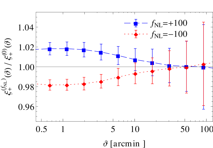
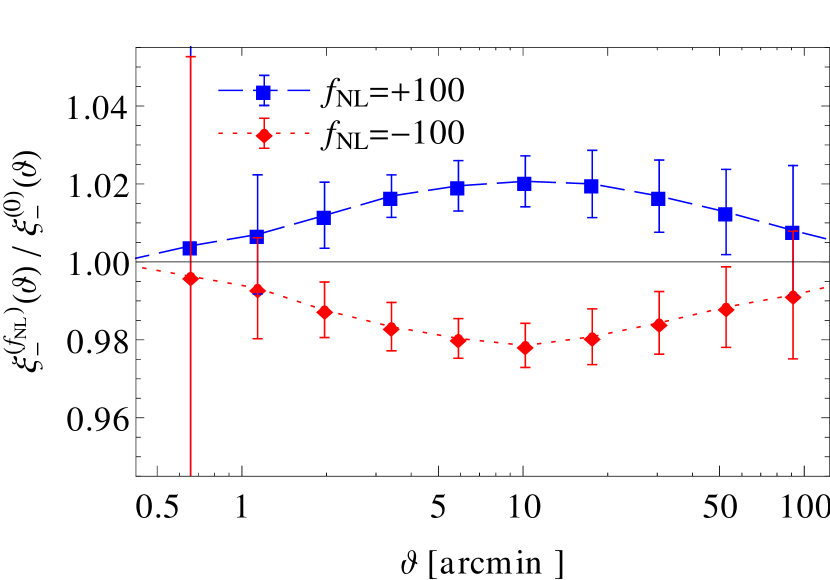
Figure 1: Cosmic shear correlations ξ±(fNL)(ϑ)superscriptsubscript𝜉plus-or-minussubscript𝑓NLitalic-ϑ\xi_{\pm}^{(f_{\text{NL}})}(\vartheta) as functions of separation ϑitalic-ϑ\vartheta for different values of non-Gaussianity fNLsubscript𝑓NLf_{\text{NL}}. Points show the relative difference between fNL0subscript𝑓NL0f_{\text{NL}}\neq 0 and fNL=0subscript𝑓NL0f_{\text{NL}}=0. Error bars indicate the statistical uncertainties due to shape noise and cosmic variance expected for large future surveys.

Figure 1 shows the relative differences in the cosmic shear correlation functions ξ+subscript𝜉\xi_{+} and ξsubscript𝜉\xi_{-} between the Gaussian case fNL=0subscript𝑓NL0f_{\text{NL}}=0 and the non-Gaussian case fNL0subscript𝑓NL0f_{\text{NL}}\neq 0. The error bars indicate the statistical errors due to the intrinsic galaxy image shapes and cosmic variance expected for a large future survey (see Section 4.2 for a more detailed discussion).

On scales ϑ<1degitalic-ϑ1deg\vartheta<1\,\mathrm{deg}, the shear correlation function ξ+(ϑ)subscript𝜉italic-ϑ\xi_{+}(\vartheta) is larger for larger fNLsubscript𝑓NLf_{\text{NL}}. The largest relative difference is visible on scales ϑ1arcminsimilar-toitalic-ϑ1arcmin\vartheta\sim 1\,\mathrm{arcmin}. The difference is only about ±2%plus-or-minuspercent2\pm 2\% for fNL=±100subscript𝑓NLplus-or-minus100f_{\text{NL}}=\pm 100, but this is large enough to be detectable in future surveys, since the errors are 1%less-than-or-similar-toabsentpercent1\lesssim 1\% at these separations, as shown in the next section. The results for ξsubscript𝜉\xi_{-} are very similar, but with the largest relative differences shifted to larger scales 10arcminsimilar-toabsent10arcmin\sim 10\,\mathrm{arcmin}.

Both ξ+subscript𝜉\xi_{+} and ξsubscript𝜉\xi_{-} are weighted projections of the three-dimensional matter correlation, with ξ+(ϑ)subscript𝜉italic-ϑ\xi_{+}(\vartheta) probing larger 3-D scales than ξ(ϑ)subscript𝜉italic-ϑ\xi_{-}(\vartheta) at the same angular scale ϑitalic-ϑ\vartheta. At redshifts z0.3similar-to𝑧0.3z\sim 0.3, where lensing is most efficient, the angular scales where the shear correlations show the largest response to fNLsubscript𝑓NLf_{\text{NL}} correspond to 3-D scales of a few hundred kpckpc\mathrm{kpc}. This result is consistent with predictions from a halo model (Smith et al. 2011). In the presence of primordial non-Gaussianity, both the abundance and density profiles of massive haloes are slightly increased/decreased for positive/negative fNLsubscript𝑓NLf_{\text{NL}}. The relative contribution of these massive halos to the matter correlation is largest at the group and cluster scales. On smaller length scales, the signal becomes dominated by the lower mass halos, for which the effects of primordial non-Gaussianity are significantly reduced. On larger scales, two-halo terms, which are also less affected by primordial non-Gaussianity, dominate the matter correlation. This signature is qualitatively mirrored in Figure 1.
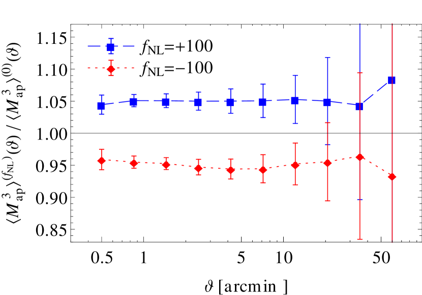
Refer to caption

Figure 2: Third-order aperture mass statistics Map3(fNL)(ϑ)superscriptdelimited-⟨⟩superscriptsubscript𝑀ap3subscript𝑓NLitalic-ϑ\bigl{\langle}{M_{\text{ap}}^{3}}\bigr{\rangle}^{(f_{\text{NL}})}(\vartheta) as function of filter scale ϑitalic-ϑ\vartheta for different values of non-Gaussianity fNLsubscript𝑓NLf_{\text{NL}}. Points show the relative difference between fNL0subscript𝑓NL0f_{\text{NL}}\neq 0 and fNL=0subscript𝑓NL0f_{\text{NL}}=0. Error bars on indicate the statistical uncertainties due to shape noise and cosmic variance expected for large future surveys.

Figure 2 shows the differences in the aperture statistics Map3(ϑ)delimited-⟨⟩superscriptsubscript𝑀ap3italic-ϑ\bigl{\langle}{M_{\text{ap}}^{3}}\bigr{\rangle}(\vartheta). Similar to the shear correlation functions, the third-order aperture mass statistics is larger for larger primordial non-Gaussianity. The relative difference in Map3(ϑ)delimited-⟨⟩superscriptsubscript𝑀ap3italic-ϑ\bigl{\langle}{M_{\text{ap}}^{3}}\bigr{\rangle}(\vartheta) is about ±5%plus-or-minuspercent5\pm 5\% for fNL±100plus-or-minussubscript𝑓NL100f_{\text{NL}}\pm 100, which is clearly larger than the statistical uncertainties of about 1%percent11\% expected for scales ϑ5arcminless-than-or-similar-toitalic-ϑ5arcmin\vartheta\lesssim 5\,\mathrm{arcmin} in large future surveys, as shown in the next section.
Refer to caption

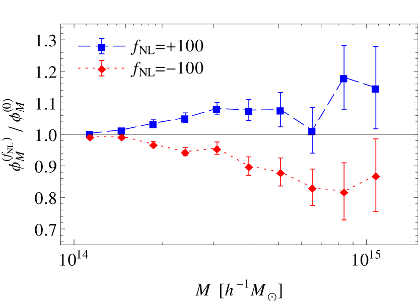
Figure 3: Shear peak abundance ϕM(fNL)(M)superscriptsubscriptitalic-ϕ𝑀subscript𝑓NL𝑀\phi_{M}^{(f_{\text{NL}})}(M) as function of peak mass M𝑀M for different values of non-Gaussianity fNLsubscript𝑓NLf_{\text{NL}}. Points show the relative difference between fNL0subscript𝑓NL0f_{\text{NL}}\neq 0 and fNL=0subscript𝑓NL0f_{\text{NL}}=0. Error bars indicate the statistical uncertainties due to shape noise and cosmic variance expected for large future surveys.

The impact of primordial non-Gaussianity on the shear peak abundance ϕM(M)subscriptitalic-ϕ𝑀𝑀\phi_{M}(M) is shown in Fig. 3. The peak abundance increases with increasing fNLsubscript𝑓NLf_{\text{NL}}. Similar results were presented in our previous study (Marian et al. 2011). The change is stronger for larger peak masses M𝑀M. For these larger masses, however, also the noise becomes larger.

4.2 Error analysis
Refer to caption

Refer to caption

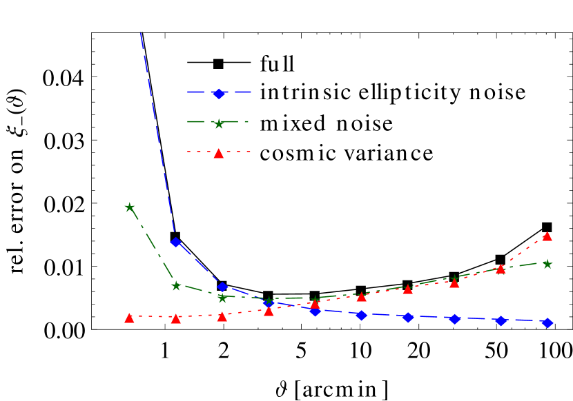
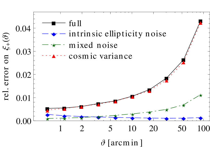
Figure 4: Expected contributions to the relative errors (symbols, connected by lines for visual guidance) on the estimates of the shear correlation functions ξ±(ϑ)subscript𝜉plus-or-minusitalic-ϑ\xi_{\pm}(\vartheta) in bins of separation ϑitalic-ϑ\vartheta: full error (squares), intrinsic ellipticity noise (diamonds), mixed noise (stars), and cosmic variance (triangles).

As discussed in Section 3.4, the uncertainties in the measured shear correlation functions can be split into a pure shape noise part, a pure cosmic variance part, and a mixed noise part due to a coupling of shape noise and shear correlations. In Fig. 4, these contributions are shown together with the full statistical uncertainties for our assumed survey. The cosmic variance dominates the error on ξ+subscript𝜉\xi_{+} on all considered scales (cf., e.g., Beynon et al. 2010). The cosmic variance sets a lower limit of 0.5%similar-toabsentpercent0.5\sim 0.5\% on the uncertainty in ξ+(ϑ)subscript𝜉italic-ϑ\xi_{+}(\vartheta) for separations ϑ1arcminsimilar-toitalic-ϑ1arcmin\vartheta\sim 1\,\mathrm{arcmin}, and of 1%greater-than-or-equivalent-toabsentpercent1\gtrsim 1\% on ϑ10arcmingreater-than-or-equivalent-toitalic-ϑ10arcmin\vartheta\gtrsim 10\,\mathrm{arcmin}. Shape noise is the dominant contribution only for ξsubscript𝜉\xi_{-} on scales ϑ2arcminless-than-or-similar-toitalic-ϑ2arcmin\vartheta\lesssim 2\,\mathrm{arcmin}. On larger scales, the cosmic variance and mixed noise dominate the error on ξsubscript𝜉\xi_{-}.

As previously mentioned, our covariance results based on the simulated 12×12deg21212superscriptdeg212\times 12\,\mathrm{deg}^{2} fields might underestimate the covariance of ξ(ϑ)subscript𝜉minus-or-plusitalic-ϑ\xi_{\mp}(\vartheta) in a full-sky survey, in particular for large separations ϑitalic-ϑ\vartheta. To check this, we also compute the expected full-sky covariance employing the normal and the log-normal approximation (Schneider et al. 2002b; Hilbert et al. 2011). The results from these analytic approximations indicate that our simulation results do not underestimate the covariance except for ξ+subscript𝜉\xi_{+} on large scales ϑ1deggreater-than-or-equivalent-toitalic-ϑ1deg\vartheta\gtrsim 1\,\mathrm{deg}, where the difference is 20%similar-toabsentpercent20\sim 20\%.

Refer to caption

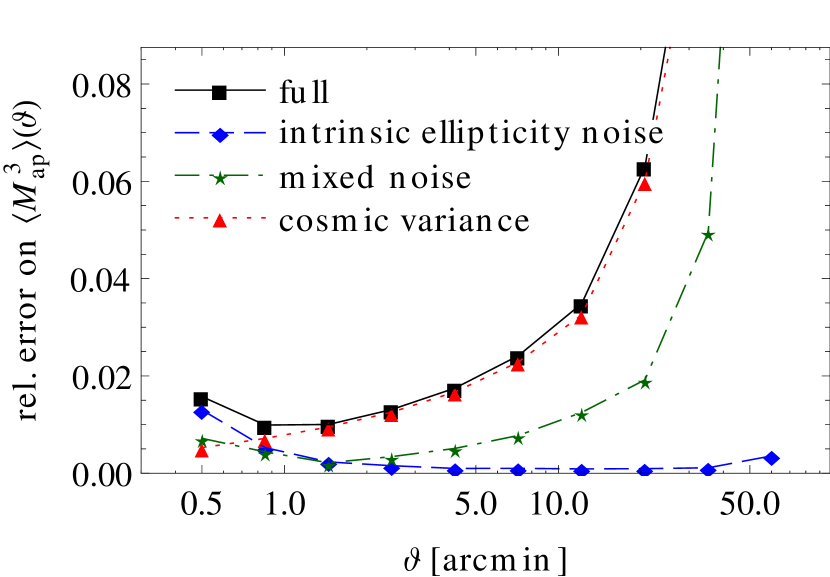
Figure 5: Expected contributions to the relative errors on the estimates of the third-order aperture mass statistics Map3(ϑ)delimited-⟨⟩superscriptsubscript𝑀ap3italic-ϑ\bigl{\langle}{M_{\text{ap}}^{3}}\bigr{\rangle}(\vartheta) for various filter scales ϑitalic-ϑ\vartheta: full error (squares), intrinsic ellipticity noise (diamonds), mixed noise (stars), and cosmic variance (triangles).

Figure 5 shows that the cosmic variance is also the dominant contribution to the error on the aperture statistic Map3(ϑ)delimited-⟨⟩superscriptsubscript𝑀ap3italic-ϑ\bigl{\langle}{M_{\text{ap}}^{3}}\bigr{\rangle}(\vartheta) on scales ϑ>1arcminitalic-ϑ1arcmin\vartheta>1\,\mathrm{arcmin}. Only for smaller filter scales, there is a significant contribution from galaxy shape noise and mixed noise.
Refer to caption

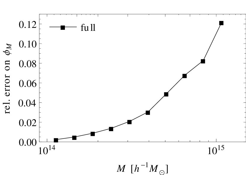
Figure 6: Expected relative errors (symbols, connected by lines for visual guidance) on the estimates of the shear peak abundance ϕM(M)subscriptitalic-ϕ𝑀𝑀\phi_{M}(M) for various peak masses M𝑀M.

The estimated errors for the shear peak abundance are shown in Figure 6. The errors are 1%similar-toabsentpercent1\sim 1\% for the bins with peak masses of a few 1014h1Msuperscript1014superscript1subscriptMdirect-product10^{14}h^{-1}\,\mathrm{M}_{\odot} or smaller, but rapidly increase to tens of percent for larger peak masses. There is no easy way to split the errors into contributions from shape noise or cosmic variance. However, by comparing results from fields with the same cosmic structure but different shape noise realizations, we find that shape noise makes a substantial contribution to the statistical errors on the peak counts even for intermediate and large peak masses. A more thorough understanding of the noise properties of the shear peak statistics is certainly worthwile in future.

4.3 The covariance of the lensing statistics
Refer to caption

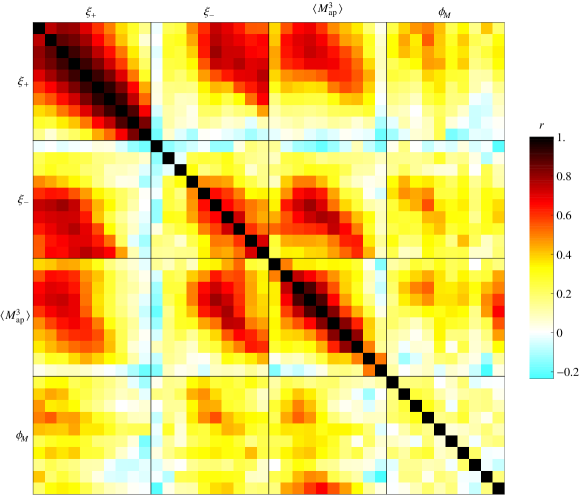
Figure 7: Correlation matrix quantifying the correlation between the entries of the full data vector, containing the shear correlations functions ξ±(θ)subscript𝜉plus-or-minus𝜃\xi_{\pm}(\theta) measured in 10 bins of pair separation θ𝜃\theta, the aperture statistics Map3(ϑ)delimited-⟨⟩superscriptsubscript𝑀ap3italic-ϑ\bigl{\langle}{M_{\text{ap}}^{3}}\bigr{\rangle}(\vartheta) measured for 10 filter scales θ𝜃\theta, and the shear peak abundance ϕM(M)subscriptitalic-ϕ𝑀𝑀\phi_{M}(M) measured in 10 bins of peak mass M𝑀M. Within each class of observables, filter masses, scales or separations increase from left to right and from top to bottom. Darker colors indicate larger absolute correlation.

The error analysis in the previous section was restricted to the autovariance of the lensing observables ξ±(θ)subscript𝜉plus-or-minus𝜃\xi_{\pm}(\theta), Map3(ϑ)delimited-⟨⟩superscriptsubscript𝑀ap3italic-ϑ\bigl{\langle}{M_{\text{ap}}^{3}}\bigr{\rangle}(\vartheta), and ϕM(M)subscriptitalic-ϕ𝑀𝑀\phi_{M}(M). Our lensing simulations allow us to estimate the full covariance between these observables, quantified by the covariance matrix 𝗖dsubscript𝗖d\boldsymbol{\mathsf{C}}_{\text{d}}. For an analysis of the correlation between the observables, we consider the correlation matrix

𝗥d=(𝗖d,ij𝗖d,ii𝗖d,jj)i,j=1Nd.subscript𝗥dsuperscriptsubscriptsubscript𝗖d𝑖𝑗subscript𝗖d𝑖𝑖subscript𝗖d𝑗𝑗𝑖𝑗1subscript𝑁d\boldsymbol{\mathsf{R}}_{\text{d}}=\left(\frac{\boldsymbol{\mathsf{C}}_{\text{d},ij}}{\sqrt{\boldsymbol{\mathsf{C}}_{\text{d},ii}\boldsymbol{\mathsf{C}}_{\text{d},jj}}}\right)_{i,j=1}^{N_{\text{d}}}. (37)

The correlation matrix is shown in Fig. 7. All ξ+subscript𝜉\xi_{+}-bins with similar separations ϑitalic-ϑ\vartheta are strongly correlated with each other. The correlation among the ξsubscript𝜉\xi_{-}-bins and among the Map3delimited-⟨⟩superscriptsubscript𝑀ap3\bigl{\langle}{M_{\text{ap}}^{3}}\bigr{\rangle}-bins is slightly smaller. There is also a substantial correlation between ξ+subscript𝜉\xi_{+}, ξsubscript𝜉\xi_{-}, and Map3delimited-⟨⟩superscriptsubscript𝑀ap3\bigl{\langle}{M_{\text{ap}}^{3}}\bigr{\rangle}. Such large correlations are expected for surveys like the one considered here, where the cosmic variance is the dominant source of uncertainties.

In contrast, there is little correlation between different bins of ϕMsubscriptitalic-ϕ𝑀\phi_{M}. The correlation between ϕMsubscriptitalic-ϕ𝑀\phi_{M} and the other lensing observables is not very large either. This indicates that by combining the shear peak statistics with the other probes, one can obtain substantially more information than one could get from either shear peaks or, e.g., cosmic shear correlations alone (as advocated by Dietrich and Hartlap 2010).

4.4 Derivatives of the lensing observables

Refer to caption

Figure 8: Derivatives of the cosmic shear correlations ξ±subscript𝜉plus-or-minus\xi_{\pm}, the aperture statistics Map3delimited-⟨⟩superscriptsubscript𝑀ap3\bigl{\langle}{M_{\text{ap}}^{3}}\bigr{\rangle}, and the shear peak abundance ϕMsubscriptitalic-ϕ𝑀\phi_{M} with respect to the non-Gaussianity parameter fNLsubscript𝑓NLf_{\text{NL}}, the mean matter density ΩmsubscriptΩm\Omega_{\text{m}}, the matter power spectrum normalization σ8subscript𝜎8\sigma_{8} and the spectral index nssubscript𝑛sn_{\text{s}}, and the equation-of-state parameter w0subscript𝑤0w_{0} of the dark energy, as estimated from our simulations (points with error bars indicating uncertainties on the estimate).

Refer to caption

Figure 9: Derivatives of the cosmic shear correlations ξ±subscript𝜉plus-or-minus\xi_{\pm} (1st and 2nd column), the aperture statistics Map3delimited-⟨⟩superscriptsubscript𝑀ap3\bigl{\langle}{M_{\text{ap}}^{3}}\bigr{\rangle} (3rd column), and the shear peak abundance ϕMsubscriptitalic-ϕ𝑀\phi_{M} (4th column) with respect to the non-Gaussianity parameter fNLsubscript𝑓NLf_{\text{NL}} (top row), the mean matter density ΩmsubscriptΩm\Omega_{\text{m}} (2nd row), the matter power spectrum normalization σ8subscript𝜎8\sigma_{8} (3rd row) and the spectral index nssubscript𝑛sn_{\text{s}} (4th row), and the equation-of-state parameter w0subscript𝑤0w_{0} of the dark energy (5th row) relative to the statistical errors σdsubscript𝜎d\sigma_{\text{d}} on the observables predicted for a large future survey (points with error bars indicating uncertainties stemming from our noisy estimates of the derivatives).

In order to translate the measurement uncertainties and correlations in the lensing observables into uncertainties and correlations in the cosmological parameters, we need to know how the observables respond to changes in the parameters. As apparent from Eq. (24), the derivatives of the model prediction with respect to the parameters are sufficient for this.

The derivatives we estimate from our simulations via finite difference are shown in Fig. 8. The Figure also shows the statistical uncertainties on our results for the derivatives stemming from our limited number of realizations. In most cases, the derivatives bear a relatively small statistical uncertainty. Only for Map3delimited-⟨⟩superscriptsubscript𝑀ap3\bigl{\langle}{M_{\text{ap}}^{3}}\bigr{\rangle} and ϕMsubscriptitalic-ϕ𝑀\phi_{M}, the uncertainties in the derivatives reach a magnitude similar to the derivatives themselves on larger aperture and mass scales.

In order to understand how much each observable contributes to the parameter constraints, and how much the uncertainties in the derivatives might affect the estimated parameter errors, we consider the individual contributions to the sum in Eq. (25). These contributions, the derivatives rescaled by the expected statistical errors on the observables due to shape noise and cosmic variance, can be considered as measures of differential signal-to-noise. They are shown in Fig. 9.

The scales with the largest contributions to constraints on fNLsubscript𝑓NLf_{\text{NL}} from ξ+subscript𝜉\xi_{+} and ξsubscript𝜉\xi_{-} are 1arcminsimilar-toabsent1arcmin\sim 1\,\mathrm{arcmin} and 10arcminsimilar-toabsent10arcmin\sim 10\,\mathrm{arcmin}, which are the scales where the relative changes in ξ+subscript𝜉\xi_{+} and ξsubscript𝜉\xi_{-} with changing fNLsubscript𝑓NLf_{\text{NL}} are largest. For Map3delimited-⟨⟩superscriptsubscript𝑀ap3\bigl{\langle}{M_{\text{ap}}^{3}}\bigr{\rangle}, the largest contributions are from scales 1arcminsimilar-toabsent1arcmin\sim 1\,\mathrm{arcmin}, where the relative errors are smallest. For ϕMsubscriptitalic-ϕ𝑀\phi_{M}, the largest contributions to constraints on fNLsubscript𝑓NLf_{\text{NL}} are not from large peak masses, where the relative change with changing fNLsubscript𝑓NLf_{\text{NL}} is largest, but from intermediate peak masses due to the much smaller noise.333 Note however that this simple consideration ignores correlations between bins.

The results for the contributions to the constraints on the other cosmological parameters are similar. In general, most constraints come from small and intermediate scales, with the largest angular and mass scales contributing relatively little. In particular, the peak counts in the small mass range appear to provide the largest contributions to constraints on the DE EOS parameter w0subscript𝑤0w_{0}.

4.5 Cosmological constraints

In this section, we discuss the cosmological constraints expected from measuring and analyzing the cosmic shear correlation functions ξ±(ϑ)subscript𝜉plus-or-minusitalic-ϑ\xi_{\pm}(\vartheta), the third-order aperture statistics Map3(ϑ)delimited-⟨⟩superscriptsubscript𝑀ap3italic-ϑ\bigl{\langle}{M_{\text{ap}}^{3}}\bigr{\rangle}(\vartheta), and the shear peak statistics ϕM(M)subscriptitalic-ϕ𝑀𝑀\phi_{M}(M) in a large future WL survey.

We restrict the analysis to flat CDM cosmologies with a dark energy with a time-independent equation of state and local-type primordial non-Gaussianity, which is the class of models covered by our suite of simulations. The considered parameters are the non-Gaussianity parameter fNLsubscript𝑓NLf_{\text{NL}}, the mean matter density ΩmsubscriptΩm\Omega_{\text{m}}, the matter power spectrum normalization σ8subscript𝜎8\sigma_{8} and spectral index nssubscript𝑛sn_{\text{s}}, and the dark-energy equation-of-state parameter w0subscript𝑤0w_{0}. Here, we concentrate on the conditional and marginal parameter constraints, as well as possible biases due to ignoring non-vanishing non-Gaussianity. The full posterior parameter covariances for the considered probes are listed in Appendix B.

4.5.1 Conditional constraints on cosmological parameters

Table 1: Conditional constraints on cosmological parameters from a large future weak lensing survey: estimated conditional posterior standard deviations σcsubscript𝜎c\sigma_{\text{c}} of the non-Gaussianity parameter fNLsubscript𝑓NLf_{\text{NL}}, the mean matter density ΩmsubscriptΩm\Omega_{\text{m}}, the normalization σ8subscript𝜎8\sigma_{8} and the spectral index nssubscript𝑛sn_{\text{s}} of the matter power spectrum, and the equation-of-state parameter w0subscript𝑤0w_{0} of the dark energy, obtained when using the cosmic shear correlations ξ±subscript𝜉plus-or-minus\xi_{\pm}, the aperture statistics Map3delimited-⟨⟩superscriptsubscript𝑀ap3\bigl{\langle}{M_{\text{ap}}^{3}}\bigr{\rangle}, or the shear peak abundance ϕMsubscriptitalic-ϕ𝑀\phi_{M} either alone or combined with each other.
σcsubscript𝜎c\sigma_{\text{c}} from\of fNLsubscript𝑓NLf_{\text{NL}} ΩmsubscriptΩm\Omega_{\text{m}} σ8subscript𝜎8\sigma_{8} nssubscript𝑛sn_{\text{s}} w0subscript𝑤0w_{0}
ξ±subscript𝜉plus-or-minus\xi_{\pm} 21 0.0006 0.0014 0.0046 0.0149
Map3delimited-⟨⟩superscriptsubscript𝑀ap3\bigl{\langle}{M_{\text{ap}}^{3}}\bigr{\rangle} 20 0.0012 0.0019 0.0089 0.0920
ϕMsubscriptitalic-ϕ𝑀\phi_{M} 17 0.0006 0.0013 0.0053 0.0136
ξ±subscript𝜉plus-or-minus\xi_{\pm} + Map3delimited-⟨⟩superscriptsubscript𝑀ap3\bigl{\langle}{M_{\text{ap}}^{3}}\bigr{\rangle} 17 0.0005 0.0013 0.0037 0.0103
ξ±subscript𝜉plus-or-minus\xi_{\pm} + ϕMsubscriptitalic-ϕ𝑀\phi_{M} 16 0.0006 0.0013 0.0043 0.0104
Map3delimited-⟨⟩superscriptsubscript𝑀ap3\bigl{\langle}{M_{\text{ap}}^{3}}\bigr{\rangle} + ϕMsubscriptitalic-ϕ𝑀\phi_{M} 17 0.0006 0.0013 0.0051 0.0128
all WL 14 0.0005 0.0012 0.0038 0.0089

Refer to caption

Figure 10: Joint conditional constraints on pairs of cosmological parameters from a large future weak lensing survey. Considered parameters are the non-Gaussianity parameter fNLsubscript𝑓NLf_{\text{NL}}, the mean matter density ΩmsubscriptΩm\Omega_{\text{m}}, the normalization σ8subscript𝜎8\sigma_{8} and the spectral index nssubscript𝑛sn_{\text{s}} of the matter power spectrum, and the equation-of-state parameter w0subscript𝑤0w_{0} of the dark energy. Shown are the estimated 68% confidence contours obtained from the cosmic shear correlations ξ±subscript𝜉plus-or-minus\xi_{\pm} (dashed lines), the aperture statistics Map3delimited-⟨⟩superscriptsubscript𝑀ap3\bigl{\langle}{M_{\text{ap}}^{3}}\bigr{\rangle} (dotted lines), the shear peak abundance ϕMsubscriptitalic-ϕ𝑀\phi_{M} (dash-dotted lines), all of these WL probes together (solid lines).

The conditional posterior uncertainties expected from our model survey on individual cosmological parameters, when flat priors are assumed, are listed in Table 1. When all other cosmological parameters are known, the cosmic shear correlations ξ±subscript𝜉plus-or-minus\xi_{\pm}, the third-order aperture statistics Map3delimited-⟨⟩superscriptsubscript𝑀ap3\bigl{\langle}{M_{\text{ap}}^{3}}\bigr{\rangle}, and the shear peak abundance ϕMsubscriptitalic-ϕ𝑀\phi_{M} each yield 1-sigma constraints of ΔfNL20similar-toΔsubscript𝑓NL20\Delta f_{\text{NL}}\sim 20, with the smallest error ΔfNL17Δsubscript𝑓NL17\Delta f_{\text{NL}}\approx 17 from ϕMsubscriptitalic-ϕ𝑀\phi_{M}. When all WL probes are combined, the conditional error ΔfNL14Δsubscript𝑓NL14\Delta f_{\text{NL}}\approx 14.

The cosmic shear correlation functions and shear peak abundance also provide similar conditional constraints on the other cosmological parameters ΩmsubscriptΩm\Omega_{\text{m}}, σ8subscript𝜎8\sigma_{8}, nssubscript𝑛sn_{\text{s}}, and w0subscript𝑤0w_{0}. The parameter constraints from the aperture statistics are generally weaker than those from ξ±subscript𝜉plus-or-minus\xi_{\pm} or ϕMsubscriptitalic-ϕ𝑀\phi_{M}. By combining two or all three of the considered WL probes, the errors on ΩmsubscriptΩm\Omega_{\text{m}}, σ8subscript𝜎8\sigma_{8}, nssubscript𝑛sn_{\text{s}}, and w0subscript𝑤0w_{0} can also be improved. The relative conditional constraints on these parameters expected from a combined analysis of all the WL probes are 0.1%1%similar-toabsentpercent0.1percent1\sim 0.1\%-1\%, as shown in Table 1.

The joint conditional constraints for pairs of cosmological parameters are illustrated in Fig. 10. For all considered WL probes, fNLsubscript𝑓NLf_{\text{NL}} shows strong (anti-)correlations with the other considered cosmological parameters. (Anti-)correlations are also visible between the other parameters, e.g. between σ8subscript𝜎8\sigma_{8} and ΩmsubscriptΩm\Omega_{\text{m}}. The constraints from combining the WL probes benefit substantially from the complementary constraints provided by the different WL probes. Combining the information from the different probes also reduces the parameter correlations.

4.5.2 Marginalized constraints on cosmological parameters

Table 2: Marginal constraints on cosmological parameters from a large future weak lensing survey: estimated posterior standard deviations σposubscript𝜎po\sigma_{\text{po}} of the non-Gaussianity parameter fNLsubscript𝑓NLf_{\text{NL}}, the mean matter density ΩmsubscriptΩm\Omega_{\text{m}}, the normalization σ8subscript𝜎8\sigma_{8} and the spectral index nssubscript𝑛sn_{\text{s}} of the matter power spectrum, and the equation-of-state parameter w0subscript𝑤0w_{0} of the dark energy, obtained when using the cosmic shear correlations ξ±subscript𝜉plus-or-minus\xi_{\pm}, the aperture statistics Map3delimited-⟨⟩superscriptsubscript𝑀ap3\bigl{\langle}{M_{\text{ap}}^{3}}\bigr{\rangle}, or the shear peak abundance ϕMsubscriptitalic-ϕ𝑀\phi_{M} either alone, all together, or all together in conjunction with results from a CMB experiment like Planck.
σposubscript𝜎po\sigma_{\text{po}} from\of fNLsubscript𝑓NLf_{\text{NL}} ΩmsubscriptΩm\Omega_{\text{m}} σ8subscript𝜎8\sigma_{8} nssubscript𝑛sn_{\text{s}} w0subscript𝑤0w_{0}
ξ±subscript𝜉plus-or-minus\xi_{\pm} 213 0.0063 0.0118 0.0258 0.1119
Map3delimited-⟨⟩superscriptsubscript𝑀ap3\bigl{\langle}{M_{\text{ap}}^{3}}\bigr{\rangle} 444 0.0102 0.0423 0.0456 0.1873
ϕMsubscriptitalic-ϕ𝑀\phi_{M} 69 0.0084 0.0147 0.0316 0.1170
ξ±subscript𝜉plus-or-minus\xi_{\pm} + Map3delimited-⟨⟩superscriptsubscript𝑀ap3\bigl{\langle}{M_{\text{ap}}^{3}}\bigr{\rangle} 141 0.0042 0.0083 0.0127 0.0770
ξ±subscript𝜉plus-or-minus\xi_{\pm} + ϕMsubscriptitalic-ϕ𝑀\phi_{M} 60 0.0020 0.0039 0.0084 0.0278
Map3delimited-⟨⟩superscriptsubscript𝑀ap3\bigl{\langle}{M_{\text{ap}}^{3}}\bigr{\rangle} + ϕMsubscriptitalic-ϕ𝑀\phi_{M} 63 0.0040 0.0072 0.0157 0.0385
all WL 53 0.0017 0.0035 0.0067 0.0263
all WL + CMB 51 0.0014 0.0034 0.0036 0.0252

Refer to caption

Figure 11: Joint marginal constraints on pairs of cosmological parameters from a large future weak lensing survey. Considered parameters are the non-Gaussianity parameter fNLsubscript𝑓NLf_{\text{NL}}, the mean matter density ΩmsubscriptΩm\Omega_{\text{m}}, the normalization σ8subscript𝜎8\sigma_{8} and the spectral index nssubscript𝑛sn_{\text{s}} of the matter power spectrum, and the equation-of-state parameter w0subscript𝑤0w_{0} of the dark energy. Shown are the estimated 68% confidence contours obtained from the cosmic shear correlations ξ±subscript𝜉plus-or-minus\xi_{\pm} (dashed lines), the aperture statistics Map3delimited-⟨⟩superscriptsubscript𝑀ap3\bigl{\langle}{M_{\text{ap}}^{3}}\bigr{\rangle} (dotted lines), the shear peak abundance ϕMsubscriptitalic-ϕ𝑀\phi_{M} (dash-dotted lines), all of these WL probes together (solid lines), or all WL probes combined with results from a Planck-like CMB experiment.

The marginal posterior standard deviations on the cosmological parameters, assuming flat priors, are shown in Table 2. The marginal constraints on fNLsubscript𝑓NLf_{\text{NL}} from Map3delimited-⟨⟩superscriptsubscript𝑀ap3\bigl{\langle}{M_{\text{ap}}^{3}}\bigr{\rangle} alone are so large (ΔfNL500Δsubscript𝑓NL500\Delta f_{\text{NL}}\approx 500) that they are practically useless due to the relatively large uncertainties in the other cosmological parameters and their correlation with fNLsubscript𝑓NLf_{\text{NL}}. The marginal errors on fNLsubscript𝑓NLf_{\text{NL}} from ξ±subscript𝜉plus-or-minus\xi_{\pm} (ΔfNL200Δsubscript𝑓NL200\Delta f_{\text{NL}}\approx 200) or ϕMsubscriptitalic-ϕ𝑀\phi_{M} (ΔfNL70Δsubscript𝑓NL70\Delta f_{\text{NL}}\approx 70) alone are much smaller than the constraints from Map3delimited-⟨⟩superscriptsubscript𝑀ap3\bigl{\langle}{M_{\text{ap}}^{3}}\bigr{\rangle} thanks to the thighter constraints on the other cosmological parameters. All WL probes combined yield a marginal error ΔfNL50Δsubscript𝑓NL50\Delta f_{\text{NL}}\approx 50, which is somewhat larger than current constraints from CMB bispectra (ΔfNL20Δsubscript𝑓NL20\Delta f_{\text{NL}}\approx 20).

The marginal errors from either the shear correlations, the aperture statistics, or the peak counts on the other cosmological parameters are 1%20%similar-toabsentpercent1percent20\sim 1\%-20\% of the fiducial values. However, combining the information from cosmic shear and the shear peak abundance yields much more competitive marginal constraints, with uncertainties much smaller than those from any of the individual WL probes. This is in accordance with findings by Dietrich and Hartlap (2010), whose study however was limited to ΩmsubscriptΩm\Omega_{\text{m}} and σ8subscript𝜎8\sigma_{8}. An additional improvement can be obtained by also adding information from the aperture statistics. The great improvement reached by combining the three WL probes compared to only analyzing any single WL probe is also evident in the joint marginal constraints shown Fig. 11.

Table 2 also lists constraints from combining the results from the WL probes with priors that CMB temperature and E-mode polarization correlation measurements with an experiment like Planck could provide for the cosmological parameters other than fNLsubscript𝑓NLf_{\text{NL}} (see Appendix A for a computation of the prior Fisher matrix). However, the improvement on the marginal uncertainties on fNLsubscript𝑓NLf_{\text{NL}} predicted from this combination is very small. The reduction expected for the uncertainties in the other parameters is not large either except for the spectral index nssubscript𝑛sn_{\text{s}}.

To assess the robustness of our estimated parameter constraints to changes of the realizations entering the covariance, we also compute the cosmological parameter constraints using the data covariance estimated from the 128 simulated fields of the fiducial zHORIZON runs. The resulting constraints are larger or smaller by up to few tens of percent, with a slight trend toward larger uncertainties for the results based on the zHORIZON covariances. For example, the marginal constraints from combining all three WL probes become: ΔfNL=50Δsubscript𝑓NL50\Delta f_{\text{NL}}=50, ΔΩm=0.0018ΔsubscriptΩm0.0018\Delta\Omega_{\text{m}}=0.0018, Δσ8=0.0038Δsubscript𝜎80.0038\Delta\sigma_{8}=0.0038, Δns=0.0084Δsubscript𝑛s0.0084\Delta n_{\text{s}}=0.0084, Δw0=0.028Δsubscript𝑤00.028\Delta w_{0}=0.028. In comparison with the results listed in Table 2, the largest difference (a 25% increase) is observed for nssubscript𝑛sn_{\text{s}}.

4.6 Biases induced by neglecting non-Gaussianity

Table 3: Biases in cosmological parameters induced by assuming the ‘wrong’ value for the primordial non-Gaussianity fNLsubscript𝑓NLf_{\text{NL}} in the analysis of a large future weak lensing survey: differences ΔΩmΔsubscriptΩm\Delta\Omega_{\text{m}}, Δσ8Δsubscript𝜎8\Delta\sigma_{8}, ΔnsΔsubscript𝑛s\Delta n_{\text{s}}, and Δw0Δsubscript𝑤0\Delta w_{0} between the expected posterior means and the ‘true’ values of the mean matter density ΩmsubscriptΩm\Omega_{\text{m}}, the normalization σ8subscript𝜎8\sigma_{8}, the spectral index nssubscript𝑛sn_{\text{s}}, and the equation-of-state parameter w0subscript𝑤0w_{0}, resp., relative to the difference ΔfNLΔsubscript𝑓NL\Delta f_{\text{NL}} between the ‘true’ value of the primordial non-Gaussianity fNLsubscript𝑓NLf_{\text{NL}} and its value assumed in the analysis.
ΔΩmΔfNLΔsubscriptΩmΔsubscript𝑓NL\dfrac{\Delta\Omega_{\text{m}}}{\Delta f_{\text{NL}}} Δσ8ΔfNLΔsubscript𝜎8Δsubscript𝑓NL\dfrac{\Delta\sigma_{8}}{\Delta f_{\text{NL}}} ΔnsΔfNLΔsubscript𝑛sΔsubscript𝑓NL\dfrac{\Delta n_{\text{s}}}{\Delta f_{\text{NL}}} Δw0ΔfNLΔsubscript𝑤0Δsubscript𝑓NL\dfrac{\Delta w_{0}}{\Delta f_{\text{NL}}}
ξ±subscript𝜉plus-or-minus\xi_{\pm} 1×1051superscript105-1\times 10^{-5} 5×1055superscript105-5\times 10^{-5} 2×1062superscript106-2\times 10^{-6} 2×1042superscript104-2\times 10^{-4}
Map3delimited-⟨⟩superscriptsubscript𝑀ap3\bigl{\langle}{M_{\text{ap}}^{3}}\bigr{\rangle} 3×1063superscript1063\times 10^{-6} 9×1059superscript105-9\times 10^{-5} 6×1056superscript105-6\times 10^{-5} 9×1059superscript1059\times 10^{-5}
ϕMsubscriptitalic-ϕ𝑀\phi_{M} 2×1052superscript1052\times 10^{-5} 1×1041superscript104-1\times 10^{-4} 5×1055superscript1055\times 10^{-5} 7×1057superscript1057\times 10^{-5}
ξ±subscript𝜉plus-or-minus\xi_{\pm} + Map3delimited-⟨⟩superscriptsubscript𝑀ap3\bigl{\langle}{M_{\text{ap}}^{3}}\bigr{\rangle} 3×1053superscript105-3\times 10^{-5} 6×1056superscript105-6\times 10^{-5} 7×1057superscript1057\times 10^{-5} 5×1045superscript104-5\times 10^{-4}
ξ±subscript𝜉plus-or-minus\xi_{\pm} + ϕMsubscriptitalic-ϕ𝑀\phi_{M} 2×1052superscript105-2\times 10^{-5} 5×1055superscript105-5\times 10^{-5} 6×1056superscript1056\times 10^{-5} 4×1044superscript1044\times 10^{-4}
Map3delimited-⟨⟩superscriptsubscript𝑀ap3\bigl{\langle}{M_{\text{ap}}^{3}}\bigr{\rangle} + ϕMsubscriptitalic-ϕ𝑀\phi_{M} 5×1065superscript1065\times 10^{-6} 8×1058superscript105-8\times 10^{-5} 7×1057superscript105-7\times 10^{-5} 3×1043superscript104-3\times 10^{-4}
all WL 2×1052superscript105-2\times 10^{-5} 6×1056superscript105-6\times 10^{-5} 4×1054superscript1054\times 10^{-5} 4×1044superscript104-4\times 10^{-4}

Refer to caption

Figure 12: Joint marginal constraints on pairs of cosmological parameters from a large future weak lensing survey: posterior means (symbols) and 68% confidence contours (lines) for the mean matter density ΩmsubscriptΩm\Omega_{\text{m}}, the normalization σ8subscript𝜎8\sigma_{8} and the spectral index nssubscript𝑛sn_{\text{s}}, and the equation-of-state parameter w0subscript𝑤0w_{0} obtained for a cosmology with ‘true’ non-Gaussianity parameter fNL=30subscript𝑓NL30f_{\text{NL}}=30 when either allowing for fNLsubscript𝑓NLf_{\text{NL}} to vary (+, solid lines), or assuming fNL=0subscript𝑓NL0f_{\text{NL}}=0 (×\times, dashed lines) in the joint WL analysis.

The constraints on the cosmological parameters predicted for a future all-sky weak lensing survey imply substantial correlations between fNLsubscript𝑓NLf_{\text{NL}} and other cosmological parameters. This raises the question whether neglecting a possible non-Gaussianity at the level of current constraints on fNLsubscript𝑓NLf_{\text{NL}} might induce a serious bias in the other cosmological parameters. Such a bias would ruin the determination of the cosmological parameters if the shift in the inferred posterior parameter confidence regions induced by neglecting non-Gaussianity were comparable to or larger than the inferred parameter uncertainties.

We study this possible bias on the basis of Eqs. (32) to (34), assuming flat priors for the cosmological parameters and the likelihood computed from our simulations. Using Eq. (33), we can compute how the inferred posterior means of the other cosmological parameters respond to a ‘wrong’ choice (i.e. assuming a value that differs from the ‘true’ value) for fNLsubscript𝑓NLf_{\text{NL}}. This response is listed in Table 3 as ratio between the induced systematic error in the cosmological parameters and the systematic error ΔfNLΔsubscript𝑓NL\Delta f_{\text{NL}} in the non-Gaussianity parameter.

For illustrative purposes, we consider a scenario where the ‘true’ non-Gaussianity fNL=30subscript𝑓NL30f_{\text{NL}}=30 (which is roughly the current best guess, Komatsu et al. 2011). The joint marginal posterior constraints on the parameters ΩmsubscriptΩm\Omega_{\text{m}}, σ8subscript𝜎8\sigma_{8}, nssubscript𝑛sn_{\text{s}}, and w0subscript𝑤0w_{0} resulting from a joint analysis of ξ±subscript𝜉plus-or-minus\xi_{\pm}, Map3delimited-⟨⟩superscriptsubscript𝑀ap3\bigl{\langle}{M_{\text{ap}}^{3}}\bigr{\rangle}, and ϕMsubscriptitalic-ϕ𝑀\phi_{M} are shown in Fig. 12 for two cases. In the first case, fNLsubscript𝑓NLf_{\text{NL}} is considered a parameter to be constrained from the data along with the other parameters. For our simple model, the resulting posterior means coincide with the ‘true’ values of the parameters. The second case assumes fNL=0subscript𝑓NL0f_{\text{NL}}=0 in the analysis. This results in different means and covariances inferred for the parameters. The resulting biases are noticeable compared to the parameter uncertainties estimated for the full model including fNLsubscript𝑓NLf_{\text{NL}}. Moreover, the analysis ignoring a possible non-Gaussianity yields not only biased estimates, but also far too optimistic uncertainties for the remaining parameters, in particular for σ8subscript𝜎8\sigma_{8} and w0subscript𝑤0w_{0}. Thus, the parameter biases are comparable to the inferred uncertainties in that case. As a result, the confidence regions inferred by an analysis ignoring non-Gaussianity do not contain the ‘true’ values of the cosmological parameters.

5 Summary and discussion

Measurements of the level of non-Gaussianity in the primordial matter density fluctuations provide valuable information for constraining models of inflation and the origin of cosmic structure. Currently the best constraints on primordial non-Gaussianity are from CMB experiments probing matter fluctuations at very high redshifts. However, lower-redshift observables could also provide competitive constraints.

In this paper, we investigated how well a large weak lensing survey probing the matter distribution at redshifts 0<z10𝑧less-than-or-similar-to10<z\lesssim 1, can constrain the level fNLsubscript𝑓NLf_{\text{NL}} of primordial non-Gaussianity of the local type. We employed a large set of N𝑁N-body simulations of structure formation in flat w𝑤wCDM cosmologies, through which we performed full gravitational ray-tracing to simulate weak lensing observations similar to those proposed for Euclid and LSST. With these WL simulations, we studied the influence of the cosmological parameters fNLsubscript𝑓NLf_{\text{NL}}, ΩmsubscriptΩm\Omega_{\text{m}}, σ8subscript𝜎8\sigma_{8}, nssubscript𝑛sn_{\text{s}}, and w0subscript𝑤0w_{0} on the cosmic shear correlation functions ξ+subscript𝜉\xi_{+} and ξsubscript𝜉\xi_{-}, the third-order aperture mass statistics Map3delimited-⟨⟩superscriptsubscript𝑀ap3\bigl{\langle}{M_{\text{ap}}^{3}}\bigr{\rangle}, and the shear peak abundance ϕMsubscriptitalic-ϕ𝑀\phi_{M}. Furthermore, we quantified the uncertainties and covariances of these WL probes, and the resulting constraints on the cosmological parameters.

We found that if all other cosmological parameters were known accurately, each of the considered WL probes could provide constraints ΔfNL20similar-toΔsubscript𝑓NL20\Delta f_{\text{NL}}\sim 20 on the non-Gaussianity parameter fNLsubscript𝑓NLf_{\text{NL}}. The constraints were much weaker (ΔfNL100500similar-toΔsubscript𝑓NL100500\Delta f_{\text{NL}}\sim 100-500), if the other cosmological parameters had to be constrained using the same WL data. However, the uncertainties in fNLsubscript𝑓NLf_{\text{NL}} could be reduced by combining information from the different WL probes.

A joint analysis of the WL probes also yields much smaller uncertainties for the other cosmological parameters than may be obtained from any of the individual WL probes. When combining the probes, the expected marginal uncertainties at 68% confidence level on the cosmological parameters were: ΔfNL50similar-toΔsubscript𝑓NL50\Delta f_{\text{NL}}\sim 50, ΔΩm0.002similar-toΔsubscriptΩm0.002\Delta\Omega_{\text{m}}\sim 0.002, Δσ80.004similar-toΔsubscript𝜎80.004\Delta\sigma_{8}\sim 0.004, Δns0.007similar-toΔsubscript𝑛s0.007\Delta n_{\text{s}}\sim 0.007, and Δw00.03similar-toΔsubscript𝑤00.03\Delta w_{0}\sim 0.03.

At this level of accuracy, neglecting non-vanishing non-Gaussianity could induce a noticeable bias in the determination of other cosmological parameters, in particular for the matter power spectrum normalization σ8subscript𝜎8\sigma_{8} or the DE EOS parameter w0subscript𝑤0w_{0}. Moreover, neglecting a possible non-Gaussianity in the analysis may lead to far too optimistic estimates for the parameter errors.

Our results for the expected conditional errors on fNLsubscript𝑓NLf_{\text{NL}} from cosmic shear are in agreement with the findings of Fedeli and Moscardini (2010), who estimated errors of a few tens considering the weak lensing power spectra. Our results for the expected constraints from shear peaks are somewhat less optimistic than the errors predicted by Maturi et al. (2011). This might be attributed to our more realistic predictions for the peak function, which we measured directly from simulated WL maps.

The analysis in Section 4.4 showed that a large part of the parameter constraints stems from the lensing signals measured on small and intermediate angular or mass scales. This highlights the importance of improving the understanding of structure formation on these smaller scales, which is required for accurate model predictions. Moreover, an improved understanding of the shape noise is needed for accurate predictions of the shear peak statistics at these scales.

Our error analysis in Section 4.2 showed that for large future WL surveys, the statistical errors on the cosmic shear correlations and the aperture statistics are cosmic-variance dominated. This implies that for these probes, reducing the shape noise, e.g. by increasing the survey depth, will not reduce the statistical errors much.

An obvious extension of this work is to take tomographic information into account. Tomography might not significantly improve the errors on fNLsubscript𝑓NLf_{\text{NL}} arising from two-point statistics like the convergence power spectrum (see Fedeli and Moscardini 2010), but it could improve the constraints from the peak abundance. It will also significantly reduce the errors on other parameters, such as the equation-of-state parameters of the Dark Energy. Such a study probably requires more simulations to obtain reliable covariances for the large data vectors arising in WL tomography.

One should also investigate more the constraints one may obtain from combining the WL probes with other probes of large scale structure (see Giannantonio et al. 2012). This will require simulations that include predictions for optical properties of galaxies or X-ray properties of clusters. Finally, a comprehensive future analysis should also consider other types of primordial non-Gaussianity and other cosmological parameters impacting structure formation.

Acknowledgments

We thank Alan Heavens, Carlos Cunha, and Peter Schneider for helpful discussions. We also thank Albert Stebbins for the constructive criticsm. SH and LM acknowledge support by the Deutsche Forschungsgemeinschaft (DFG) through the Priority Programme 1177 ‘Galaxy Evolution’ (SCHN 342/6 and WH 6/3), through the Transregional Collaborative Research Centre TRR 33 ‘The Dark Universe’. and through the grant MA 4967/1-1. SH also acknowledges support by the National Science Foundation (NSF) grant number AST-0807458-002. RES was partly supported by the Swiss National Foundation under contract 200021-116696/1 and the WCU grant R32-2008-000-10130-0. RES also acknowledges support from a Marie Curie Reintegration Grant and the Alexander von Humboldt Foundation. VD acknowledges support by the Swiss National Foundation and by the University of Zürich through FK UZH 57184001.

References

  • Acquaviva et al. (2003) Acquaviva V., Bartolo N., Matarrese S., Riotto A., 2003, Nuclear Physics B, 667, 119
  • Amara and Refregier (2004) Amara A., Refregier A., 2004, MNRAS, 351, 375
  • Anderson (2003) Anderson T.W., 2003, An introduction to multivariate statistical analysis, John Wiley & Sons, Inc., Hoboken, New Jersey, 3 edn.
  • Baldauf et al. (2011) Baldauf T., Seljak U., Senatore L., 2011, JCAP, 4, 6
  • Bartelmann and Schneider (2001) Bartelmann M., Schneider P., 2001, Phys. Rep., 340, 291
  • Beynon et al. (2010) Beynon E., Bacon D.J., Koyama K., 2010, MNRAS, 403, 353
  • Blandford and Narayan (1986) Blandford R., Narayan R., 1986, ApJ, 310, 568
  • Brainerd et al. (1996) Brainerd T.G., Blandford R.D., Smail I., 1996, ApJ, 466, 623
  • Brandenberger et al. (2007) Brandenberger R.H., Nayeri A., Patil S.P., Vafa C., 2007, International Journal of Modern Physics A, 22, 3621
  • Creminelli and Zaldarriaga (2004) Creminelli P., Zaldarriaga M., 2004, JCAP, 10, 6
  • Dalal et al. (2008) Dalal N., Doré O., Huterer D., Shirokov A., 2008, Phys. Rev. D, 77, 123514
  • Desjacques et al. (2009) Desjacques V., Seljak U., Iliev I.T., 2009, MNRAS, 396, 85
  • Dietrich and Hartlap (2010) Dietrich J.P., Hartlap J., 2010, MNRAS, 402, 1049
  • Eisenstein et al. (1999) Eisenstein D.J., Hu W., Tegmark M., 1999, ApJ, 518, 2
  • Fedeli and Moscardini (2010) Fedeli C., Moscardini L., 2010, MNRAS, 405, 681
  • Fedeli et al. (2011) Fedeli C., Pace F., Moscardini L., Grossi M., Dolag K., 2011, MNRAS, 416, 3098
  • Giannantonio et al. (2012) Giannantonio T., Porciani C., Carron J., Amara A., Pillepich A., 2012, MNRAS, 422, 2854
  • Hamana et al. (2004) Hamana T., Takada M., Yoshida N., 2004, MNRAS, 350, 893
  • Hartlap et al. (2007) Hartlap J., Simon P., Schneider P., 2007, A&A, 464, 399
  • Hilbert et al. (2009) Hilbert S., Hartlap J., White S.D.M., Schneider P., 2009, A&A, 499, 31
  • Hilbert et al. (2011) Hilbert S., Hartlap J., Schneider P., 2011, A&A, 536, A85
  • Hu and Sawicki (2007) Hu W., Sawicki I., 2007, Phys. Rev. D, 76, 104043
  • Jain et al. (2000) Jain B., Seljak U., White S., 2000, ApJ, 530, 547
  • Jeong et al. (2009) Jeong D., Komatsu E., Jain B., 2009, Phys. Rev. D, 80, 123527
  • Kaiser (1992) Kaiser N., 1992, ApJ, 388, 272
  • Khoury et al. (2001) Khoury J., Ovrut B.A., Steinhardt P.J., Turok N., 2001, Phys. Rev. D, 64, 123522
  • Kilbinger and Schneider (2005) Kilbinger M., Schneider P., 2005, A&A, 442, 69
  • Komatsu et al. (2011) Komatsu E., Smith K.M., Dunkley J., The WMAP Team, 2011, ApJS, 192, 18
  • Komatsu et al. (2009) Komatsu E., et al., 2009, ApJS, 180, 330
  • Krause and Hirata (2010) Krause E., Hirata C.M., 2010, A&A, 523, A28
  • Kuijken (2007) Kuijken K., 2007, Highlights of Astronomy, 14, 580
  • Laureijs et al. (2011) Laureijs R., et al., 2011, Euclid Definition Study Report, Tech. rep., ESA
  • Lewis et al. (2000) Lewis A., Challinor A., Lasenby A., 2000, Astrophys. J., 538, 473
  • Lo Verde et al. (2008) Lo Verde M., Miller A., Shandera S., Verde L., 2008, Journal of Cosmology and Astro-Particle Physics, 4, 14
  • LSST Science Collaborations and LSST Project (2009) LSST Science Collaborations and LSST Project, 2009, LSST Science Book, Version 2.0, arXiv:0912.0201, http://www.lsst.org/lsst/scibook
  • Maldacena (2003) Maldacena J., 2003, Journal of High Energy Physics, 5, 13
  • Marian and Bernstein (2006) Marian L., Bernstein G.M., 2006, Phys. Rev. D, 73, 123525
  • Marian et al. (2009) Marian L., Smith R.E., Bernstein G.M., 2009, ApJ, 698, L33
  • Marian et al. (2011) Marian L., Hilbert S., Smith R.E., Schneider P., Desjacques V., 2011, ApJ, 728, L13
  • Marian et al. (2012) Marian L., Smith R.E., Hilbert S., Schneider P., 2012, MNRAS, 423, 1711
  • Matarrese et al. (2000) Matarrese S., Verde L., Jimenez R., 2000, ApJ, 541, 10
  • Maturi et al. (2011) Maturi M., Fedeli C., Moscardini L., 2011, MNRAS, 416, 2527
  • Miyazaki et al. (2002) Miyazaki S., et al., 2002, ApJ, 580, L97
  • Mukhanov and Chibisov (1981) Mukhanov V.F., Chibisov G.V., 1981, Soviet Jour. of Exper. and Theor. Phys. Lett., 33, 532
  • Navarro et al. (1997) Navarro J.F., Frenk C.S., White S.D.M., 1997, ApJ, 490, 493
  • Nishimichi et al. (2010) Nishimichi T., Taruya A., Koyama K., Sabiu C., 2010, JCAP, 7, 2
  • Oguri and Takada (2011) Oguri M., Takada M., 2011, Phys. Rev. D, 83, 023008
  • Pace et al. (2011) Pace F., Moscardini L., Bartelmann M., Branchini E., Dolag K., Grossi M., Matarrese S., 2011, MNRAS, 411, 595
  • Pillepich et al. (2010) Pillepich A., Porciani C., Hahn O., 2010, MNRAS, 402, 191
  • Press et al. (1992) Press W.H., Teukolsky S.A., Vetterling W.T., Flannery B.P., 1992, Numerical recipes in FORTRAN. The art of scientific computing, Cambridge: University Press, 2nd edn.
  • Schäfer et al. (2012) Schäfer B.M., Grassi A., Gerstenlauer M., Byrnes C.T., 2012, MNRAS, 421, 797
  • Schneider et al. (1998) Schneider P., van Waerbeke L., Jain B., Kruse G., 1998, MNRAS, 296, 873
  • Schneider et al. (2002a) Schneider P., van Waerbeke L., Kilbinger M., Mellier Y., 2002a, A&A, 396, 1
  • Schneider et al. (2002b) Schneider P., van Waerbeke L., Mellier Y., 2002b, A&A, 389, 729
  • Schneider et al. (2005) Schneider P., Kilbinger M., Lombardi M., 2005, A&A, 431, 9
  • Schneider et al. (2006) Schneider P., Kochanek C., Wambsganss J., 2006, Gravitational Lensing: Strong, Weak and Micro, Saas-Fee Advanced Course 33, Springer, Berlin
  • Sefusatti and Komatsu (2007) Sefusatti E., Komatsu E., 2007, Phys. Rev. D, 76, 083004
  • Sefusatti et al. (2012) Sefusatti E., Crocce M., Desjacques V., 2012, MNRAS, 425, 2903
  • Seto (2001) Seto N., 2001, ApJ, 553, 488
  • Smith (2009) Smith R.E., 2009, MNRAS, 400, 851
  • Smith et al. (2011) Smith R.E., Desjacques V., Marian L., 2011, Phys. Rev. D, 83, 043526
  • Springel (2005) Springel V., 2005, MNRAS, 364, 1105
  • Takada and Jain (2009) Takada M., Jain B., 2009, MNRAS, 395, 2065
  • The Dark Energy Survey Collaboration (2005) The Dark Energy Survey Collaboration, 2005, The Dark Energy Survey, ArXiv e-prints, astro-ph/0510346
  • The Planck Collaboration (2006) The Planck Collaboration, 2006, The Scientific Programme of Planck, ArXiv eprints, arXiv:astro-ph/0604069

Appendix A Planck Fisher matrix

A.1 Computing the CMB matrix

In computing the Planck Fisher matrix we follow the methodology described in Eisenstein et al. (1999) and for the specific implementation we follow Takada and Jain (2009). We thus assume that the CMB temperature and polarization spectra constrain 9 parameters, and for our calculations we set their fiducial values to be those from the recent WMAP7 analysis (Komatsu et al. 2011). The fiducial parameters are: dark energy EOS parameters w0=1.0subscript𝑤01.0w_{0}=-1.0 and wa=0.0subscript𝑤𝑎0.0w_{a}=0.0; the density parameter for dark energy ΩDE=0.7274subscriptΩDE0.7274\Omega_{\mathrm{DE}}=0.7274; the CDM and baryon density parameters scaled by the square of the dimensionless Hubble parameter wc=Ωch2=0.1125subscript𝑤csubscriptΩcsuperscript20.1125w_{\mathrm{c}}=\Omega_{\mathrm{c}}h^{2}=0.1125 and wb=Ωbh2=0.0226subscript𝑤bsubscriptΩbsuperscript20.0226w_{\mathrm{b}}=\Omega_{\mathrm{b}}h^{2}=0.0226 (h=H0/[100kms1Mpc1]subscript𝐻0delimited-[]100kmsuperscripts1superscriptMpc1h=H_{0}/[100\mathrm{kms^{-1}Mpc^{-1}}]); and the primordial spectral index of scalar perturbations ns=0.963subscript𝑛s0.963n_{\mathrm{s}}=0.963; the primordial amplitude of scalar perturbations As=2.173×10⁹subscript𝐴s2.173superscript109A_{\mathrm{s}}=2.173\times 10^{-9}; the running of the spectral index α=0.0𝛼0.0\alpha=0.0; and the optical depth to the last scattering surface τ=0.087𝜏0.087\tau=0.087. Hence we may write our vector of parameters:

𝒑𝗍=(w0,wa,ΩDE,wc,wb,τ,ns,As,α)𝗍.superscriptsubscript𝒑𝗍superscriptsubscript𝑤0subscript𝑤𝑎subscriptΩDEsubscript𝑤csubscript𝑤b𝜏subscript𝑛ssubscript𝐴s𝛼𝗍\boldsymbol{p}_{-}^{\mathsf{t}}=(w_{0},w_{a},\Omega_{\mathrm{DE}},w_{\mathrm{c}},w_{\mathrm{b}},\tau,n_{\mathrm{s}},A_{\mathrm{s}},\alpha)^{\mathsf{t}}. (38)

Whilst the CMB does constrain fNLsubscript𝑓NLf_{\text{NL}} through the temperature and polarization bispectra, here we are only interested in assessing the potential of weak lensing to place constraints on fNLsubscript𝑓NLf_{\text{NL}}. We therefore extend the vector 𝒑subscript𝒑\boldsymbol{p}_{-} to the 10-dimensional vector:

𝒑𝒑=(w0,,α,fNL)𝗍.maps-tosubscript𝒑𝒑superscriptsubscript𝑤0𝛼subscript𝑓NL𝗍\boldsymbol{p}_{-}\mapsto\boldsymbol{p}=(w_{0},\ldots,\alpha,f_{\text{NL}})^{\mathsf{t}}. (39)

The CMB Fisher matrix can be written as (Eisenstein et al. 1999):

𝐅pαpβ=X,YC,XpαCov1[C,X,C,Y]C,Ypβ,subscript𝐅subscript𝑝𝛼subscript𝑝𝛽subscriptsubscript𝑋𝑌subscript𝐶𝑋subscript𝑝𝛼superscriptCov1subscript𝐶𝑋subscript𝐶𝑌subscript𝐶𝑌subscript𝑝𝛽{\mathbf{F}}_{p_{\alpha}p_{\beta}}=\sum_{\ell}\sum_{X,Y}\frac{\partial C_{\ell,X}}{\partial p_{\alpha}}\mathrm{Cov}^{-1}\left[C_{\ell,X},C_{\ell,Y}\right]\frac{\partial C_{\ell,Y}}{\partial p_{\beta}}\ , (40)

where {X,Y}{TT,EE,TE}𝑋𝑌TTEETE\{X,Y\}\in\{\mathrm{TT},\,\mathrm{EE},\,\mathrm{TE}\}, where C,TTsubscript𝐶TTC_{\ell,\rm TT} is the temperature power spectrum, C,EEsubscript𝐶EEC_{\ell,\rm EE} is the E-mode polarization power spectrum, C,TEsubscript𝐶TEC_{\ell,\rm TE} is the temperature-E-mode polarization cross-power spectrum. We have been conservative and assumed that there will be no significant information from the C,BBsubscript𝐶BBC_{\ell,\rm BB}, the B-mode polarization power spectrum. We compute all CMB spectra using CAMB (Lewis et al. 2000) and use the additional module for time evolving dark energy models (Hu and Sawicki 2007). We include information from all multipoles in the range (2<<1500215002<\ell<1500).

The covariance matrices for these observables are:

Cov[C,TT,C,TT]Covsubscript𝐶TTsubscript𝐶TT\displaystyle\operatorname{Cov}\left[C_{\ell,{\mathrm{TT}}},C_{\ell,{\mathrm{TT}}}\right] =1fsky22+1[C,TT+N,TT]2;absent1subscript𝑓sky221superscriptdelimited-[]subscript𝐶TTsubscript𝑁TT2\displaystyle=\frac{1}{f_{\mathrm{sky}}}\frac{2}{2\ell+1}\left[C_{\ell,{\mathrm{TT}}}+N_{\ell,{\mathrm{TT}}}\right]^{2}\ ; (41)
Cov[C,TT,C,EE]Covsubscript𝐶TTsubscript𝐶EE\displaystyle\operatorname{Cov}\left[C_{\ell,{\mathrm{TT}}},C_{\ell,{\mathrm{EE}}}\right] =1fsky22+1C,TE2;absent1subscript𝑓sky221superscriptsubscript𝐶TE2\displaystyle=\frac{1}{f_{\mathrm{sky}}}\frac{2}{2\ell+1}C_{\ell,{\mathrm{TE}}}^{2}\ ; (42)
Cov[C,TT,C,TE]Covsubscript𝐶TTsubscript𝐶TE\displaystyle\operatorname{Cov}\left[C_{\ell,{\mathrm{TT}}},C_{\ell,{\mathrm{TE}}}\right] =1fsky22+1C,TE[C,TT+N,TT];absent1subscript𝑓sky221subscript𝐶TEdelimited-[]subscript𝐶TTsubscript𝑁TT\displaystyle=\frac{1}{f_{\mathrm{sky}}}\frac{2}{2\ell+1}C_{\ell,{\mathrm{TE}}}\left[C_{\ell,{\mathrm{TT}}}+N_{\ell,{\mathrm{TT}}}\right]\ ; (43)
Cov[C,EE,C,EE]Covsubscript𝐶EEsubscript𝐶EE\displaystyle\operatorname{Cov}\left[C_{\ell,{\mathrm{EE}}},C_{\ell,{\mathrm{EE}}}\right] =1fsky22+1[C,EE+N,EE]2;absent1subscript𝑓sky221superscriptdelimited-[]subscript𝐶EEsubscript𝑁EE2\displaystyle=\frac{1}{f_{\mathrm{sky}}}\frac{2}{2\ell+1}\left[C_{\ell,{\mathrm{EE}}}+N_{\ell,{\mathrm{EE}}}\right]^{2}\ ; (44)
Cov[C,EE,C,TE]Covsubscript𝐶EEsubscript𝐶TE\displaystyle\operatorname{Cov}\left[C_{\ell,{\mathrm{EE}}},C_{\ell,{\mathrm{TE}}}\right] =1fsky22+1C,TE[C,EE+N,EE];absent1subscript𝑓sky221subscript𝐶TEdelimited-[]subscript𝐶EEsubscript𝑁EE\displaystyle=\frac{1}{f_{\mathrm{sky}}}\frac{2}{2\ell+1}C_{\ell,{\mathrm{TE}}}\left[C_{\ell,{\mathrm{EE}}}+N_{\ell,{\mathrm{EE}}}\right]\ ; (45)
Cov[C,TE,C,TE]Covsubscript𝐶TEsubscript𝐶TE\displaystyle\operatorname{Cov}\left[C_{\ell,{\mathrm{TE}}},C_{\ell,{\mathrm{TE}}}\right] =1fsky12+1[C,TE2+\displaystyle=\frac{1}{f_{\mathrm{sky}}}\frac{1}{2\ell+1}\left[C_{\ell,{\mathrm{TE}}}^{2}+\right.
(C,EE+N,TT)(C,EE+N,EE)].\displaystyle\quad\left.(C_{\ell,{\mathrm{EE}}}+N_{\ell,{\mathrm{TT}}})(C_{\ell,{\mathrm{EE}}}+N_{\ell,{\mathrm{EE}}})\right]\ . (46)

In the above fskysubscript𝑓skyf_{\mathrm{sky}} is the fraction of sky that is surveyed and usable for science, and we take fsky=0.8subscript𝑓sky0.8f_{\mathrm{sky}}=0.8. The terms N,TTsubscript𝑁TTN_{\ell,{\mathrm{TT}}} and N,EEsubscript𝑁EEN_{\ell,{\mathrm{EE}}} denote the beam-noise in the temperature and polarization detectors, respectively. These can be expressed as:

N,TTsubscript𝑁TT\displaystyle N_{\ell,{\mathrm{TT}}} =[wTTWBeam2()]1absentsuperscriptdelimited-[]subscript𝑤TTsubscriptsuperscript𝑊2Beam1\displaystyle=\left[w_{{\mathrm{TT}}}W^{2}_{\mathrm{Beam}}(\ell)\right]^{-1} (47)
N,EEsubscript𝑁EE\displaystyle N_{\ell,{\mathrm{EE}}} =[wEEWBeam2()]1,absentsuperscriptdelimited-[]subscript𝑤EEsubscriptsuperscript𝑊2Beam1\displaystyle=\left[w_{{\mathrm{EE}}}W^{2}_{\mathrm{Beam}}(\ell)\right]^{-1}\ , (48)

where wTT=[ΔTθBeam]1subscript𝑤TTsuperscriptdelimited-[]subscriptΔTsubscript𝜃Beam1w_{{\mathrm{TT}}}=\left[\Delta_{\mathrm{T}}\theta_{\mathrm{Beam}}\right]^{-1} and wEE=[ΔEθBeam]1subscript𝑤EEsuperscriptdelimited-[]subscriptΔEsubscript𝜃Beam1w_{{\mathrm{EE}}}=\left[\Delta_{\mathrm{E}}\theta_{\mathrm{Beam}}\right]^{-1}. The beam window function has the form:

WBeam2()=exp[(+1)σBeam2];σBeamθBeam8log2.formulae-sequencesubscriptsuperscript𝑊2Beam1subscriptsuperscript𝜎2Beamsubscript𝜎Beamsubscript𝜃Beam82W^{2}_{\mathrm{Beam}}(\ell)=\exp\left[-\ell(\ell+1)\sigma^{2}_{\mathrm{Beam}}\right];\quad\sigma_{\mathrm{Beam}}\equiv\frac{\theta_{\mathrm{Beam}}}{\sqrt{8\log 2}}\ . (49)

For the Planck experiment we assume that we have a single frequency band for science (143 GHz), and for this channel the following parameters apply (The Planck Collaboration 2006): angular resolution of the beam θBeam=7.1subscript𝜃Beamsuperscript7.1\theta_{\mathrm{Beam}}=7.1^{\prime} [FWHM]; the beam intensity is ΔT=2.2(TCMB/1K)[μK]subscriptΔT2.2subscript𝑇CMB1Kdelimited-[]𝜇K\Delta_{\mathrm{T}}=2.2\,(T_{\mathrm{CMB}}/1\mathrm{K})\,[\mu\rm K], ΔE=4.2(TCMB/1K)[μK]subscriptΔE4.2subscript𝑇CMB1Kdelimited-[]𝜇K\Delta_{\mathrm{E}}=4.2\,(T_{\mathrm{CMB}}/1\mathrm{K})\,[\mu\rm K]. We take the temperature of the CMB to be T=2.726K𝑇2.726KT=2.726\mathrm{K}.

A.2 Transforming from CMB to Weak Lensing parameters

In the lensing simulations, we have considered how the weak lensing signal depends on the parameters, {w0,Ωm,ns,σ8,fNL}subscript𝑤0subscriptΩmsubscript𝑛ssubscript𝜎8subscript𝑓NL\{w_{0},\Omega_{\mathrm{m}},n_{\mathrm{s}},\sigma_{8},f_{\text{NL}}\}. Let us rewrite our original 10-D parameter set in terms of a new 10-D parameters set. Therefore let us consider the transformation:

𝒑=(w0,wa,ΩDE,wc,wb,τ,ns,As,α,fNL)𝗍𝒒=(w0,wa,Ωm,h,fb,τ,ns,σ8,α,fNL)𝗍.𝒑superscriptsubscript𝑤0subscript𝑤𝑎subscriptΩDEsubscript𝑤csubscript𝑤b𝜏subscript𝑛ssubscript𝐴s𝛼subscript𝑓NL𝗍maps-to𝒒superscriptsubscript𝑤0subscript𝑤𝑎subscriptΩmsubscript𝑓𝑏𝜏subscript𝑛ssubscript𝜎8𝛼subscript𝑓NL𝗍\begin{split}\boldsymbol{p}&=(w_{0},w_{a},\Omega_{\mathrm{DE}},w_{\mathrm{c}},w_{\mathrm{b}},\tau,n_{\mathrm{s}},A_{\mathrm{s}},\alpha,f_{\text{NL}})^{\mathsf{t}}\\ \mapsto\boldsymbol{q}&=(w_{0},w_{a},\Omega_{\mathrm{m}},h,f_{b},\tau,n_{\mathrm{s}},\sigma_{8},\alpha,f_{\text{NL}})^{\mathsf{t}}.\end{split} (50)

Six of the parameters are unchanged from the original set. The remaining four are related to the original parameters in the following way:

ΩmsubscriptΩm\displaystyle\Omega_{\mathrm{m}} =1ΩDE;absent1subscriptΩDE\displaystyle=1-\Omega_{\mathrm{DE}}\ ; (51)
fbsubscript𝑓𝑏\displaystyle f_{b} =wbwb+wc;absentsubscript𝑤bsubscript𝑤bsubscript𝑤c\displaystyle=\frac{w_{\mathrm{b}}}{w_{\mathrm{b}}+w_{\mathrm{c}}}\ ; (52)
h\displaystyle h =wb+wc1ΩDE;absentsubscript𝑤bsubscript𝑤c1subscriptΩDE\displaystyle=\sqrt{\frac{w_{\mathrm{b}}+w_{\mathrm{c}}}{1-\Omega_{\mathrm{DE}}}}\ ; (53)
σ8subscript𝜎8\displaystyle\sigma_{8} =[d3𝒌(2π)3P(k|𝒑)W(kR)2]1/2,absentsuperscriptdelimited-[]superscriptd3𝒌superscript2𝜋3𝑃conditional𝑘𝒑𝑊superscript𝑘𝑅212\displaystyle=\left[\int\frac{{\mathrm{d}^{3}\boldsymbol{k}}}{(2\pi)^{3}}P(k|\boldsymbol{p})W(kR)^{2}\right]^{1/2}, (54)

where P(k|𝒑)𝑃conditional𝑘𝒑P(k|\boldsymbol{p}) is the matter power spectrum, which depends on parameters pαsubscript𝑝𝛼p_{\alpha}, and where the real space, spherical top-hat filter function has the form Wk(y)=3[sinyycosy]/y3subscript𝑊𝑘𝑦3delimited-[]𝑦𝑦𝑦superscript𝑦3W_{k}(y)=3[\sin y-y\cos y]/y^{3}, with ykR𝑦𝑘𝑅y\equiv kR and R=8Mpc𝑅8MpcR=8\mathrm{Mpc}.

We now need to construct the matrix 𝝠𝝠\boldsymbol{\mathsf{\Lambda}}, i.e. the partial derivatives of the old parameters with respect to the new parameters. From Eqns (51)–(54) we have qa=Ga(𝒑)subscript𝑞𝑎subscript𝐺𝑎𝒑q_{a}=G_{a}(\boldsymbol{p}), however in order to perform the partial derivatives we actually require the inverse of these relations, i.e. pa=Ga1(𝒒)subscript𝑝𝑎superscriptsubscript𝐺𝑎1𝒒p_{a}=G_{a}^{-1}(\boldsymbol{q}). In some cases these inverse relations may easily be determined, e.g. Eq. (51). However, in other cases no analytic inverse exists, e.g. Eq. (54). A simple way around this problem is through recalling the following:

αpμqαqαpν=δμνKsubscript𝛼subscript𝑝𝜇subscript𝑞𝛼subscript𝑞𝛼subscript𝑝𝜈subscriptsuperscript𝛿𝐾𝜇𝜈\sum_{\alpha}\frac{\partial p_{\mu}}{\partial q_{\alpha}}\frac{\partial q_{\alpha}}{\partial p_{\nu}}=\delta^{K}_{\mu\nu} (55)

Or in other terms,

αΛμαqαpν=αΛμαΛαν1=δμνKsubscript𝛼subscriptΛ𝜇𝛼subscript𝑞𝛼subscript𝑝𝜈subscript𝛼subscriptΛ𝜇𝛼subscriptsuperscriptΛ1𝛼𝜈subscriptsuperscript𝛿𝐾𝜇𝜈\sum_{\alpha}\Lambda_{\mu\alpha}\frac{\partial q_{\alpha}}{\partial p_{\nu}}=\sum_{\alpha}\Lambda_{\mu\alpha}\Lambda^{-1}_{\alpha\nu}=\delta^{K}_{\mu\nu} (56)

Hence, with qα/pνΛα,ν1subscript𝑞𝛼subscript𝑝𝜈subscriptsuperscriptΛ1𝛼𝜈{\partial q_{\alpha}}/{\partial p_{\nu}}\equiv\Lambda^{-1}_{\alpha,\nu}, we may then simply compute 𝝠𝝠\boldsymbol{\mathsf{\Lambda}}, through: 𝝠=(𝝠1)1𝝠superscriptsuperscript𝝠11\boldsymbol{\mathsf{\Lambda}}=\bigl{(}\boldsymbol{\mathsf{\Lambda}}^{-1}\bigr{)}^{-1}.

Let us therefore form the matrix Λ1superscriptΛ1\Lambda^{-1}. For the case of the five untransformed parameters, we have Λαβ1=δαβKsubscriptsuperscriptΛ1𝛼𝛽subscriptsuperscript𝛿𝐾𝛼𝛽\Lambda^{-1}_{\alpha\beta}=\delta^{K}_{\alpha\beta}. However, for the other four parameters, the situation is more complex and the non-trivial elements are:

ΩmΩDEsubscriptΩmsubscriptΩDE\displaystyle\frac{\partial\Omega_{\mathrm{m}}}{\partial\Omega_{\mathrm{DE}}} =1;absent1\displaystyle=-1\ ; (57)
fbwcsubscript𝑓𝑏subscript𝑤c\displaystyle\frac{\partial f_{b}}{\partial w_{\mathrm{c}}} =wb[wc+wb]2;absentsubscript𝑤bsuperscriptdelimited-[]subscript𝑤csubscript𝑤b2\displaystyle=-\frac{w_{\mathrm{b}}}{[w_{\mathrm{c}}+w_{\mathrm{b}}]^{2}}\ ; (58)
fbwbsubscript𝑓𝑏subscript𝑤b\displaystyle\frac{\partial f_{b}}{\partial w_{\mathrm{b}}} =wc[wc+wb]2;absentsubscript𝑤csuperscriptdelimited-[]subscript𝑤csubscript𝑤b2\displaystyle=\frac{w_{\mathrm{c}}}{[w_{\mathrm{c}}+w_{\mathrm{b}}]^{2}}\ ; (59)
hΩDEsubscriptΩDE\displaystyle\frac{\partial h}{\partial\Omega_{\mathrm{DE}}} =12wc+wb(1ΩDE)3;absent12subscript𝑤csubscript𝑤bsuperscript1subscriptΩDE3\displaystyle=\frac{1}{2}\sqrt{\frac{w_{\mathrm{c}}+w_{\mathrm{b}}}{(1-\Omega_{\mathrm{DE}})^{3}}}\ ; (60)
hwcsubscript𝑤c\displaystyle\frac{\partial h}{\partial w_{\mathrm{c}}} =12[(1ΩDE)(wb+w+c)]1/2;absent12superscriptdelimited-[]1subscriptΩDEsubscript𝑤b𝑤𝑐12\displaystyle=\frac{1}{2}\left[(1-\Omega_{\mathrm{DE}})(w_{\mathrm{b}}+w+c)\right]^{-1/2}\ ; (61)
σ8pαsubscript𝜎8subscript𝑝𝛼\displaystyle\frac{\partial\sigma_{8}}{\partial p_{\alpha}} =12σ8σ82pα=12σ8d3𝒌(2π)3P(k|𝒑)pαW(kR)2.absent12subscript𝜎8superscriptsubscript𝜎82subscript𝑝𝛼12subscript𝜎8superscriptd3𝒌superscript2𝜋3𝑃conditional𝑘𝒑subscript𝑝𝛼𝑊superscript𝑘𝑅2\displaystyle=\frac{1}{2\sigma_{8}}\frac{\partial\sigma_{8}^{2}}{\partial p_{\alpha}}=\frac{1}{2\sigma_{8}}\int\frac{{\mathrm{d}^{3}\boldsymbol{k}}}{(2\pi)^{3}}\frac{\partial P(k|\boldsymbol{p})}{\partial p_{\alpha}}W(kR)^{2}\ . (62)

Note, at leading order in fNLsubscript𝑓NLf_{\text{NL}} we have, σ8/fNL=0subscript𝜎8subscript𝑓NL0\partial\sigma_{8}/\partial f_{\text{NL}}=0. In order to compute the derivatives σ8/pαsubscript𝜎8subscript𝑝𝛼{\partial\sigma_{8}}/{\partial p_{\alpha}} we use the package CAMB. Besides the generation of various CMB power spectra, this package can output the present day linear theory matter power spectra P(k|𝒑)𝑃conditional𝑘𝒑P(k|\boldsymbol{p}). The derivatives are then determined numerically using the standard estimator for two sided derivatives.

Table 4: Covariance 𝗖prsubscript𝗖pr\boldsymbol{\mathsf{C}}_{\text{pr}} of the non-Gaussianity parameter fNLsubscript𝑓NLf_{\text{NL}}, the mean matter density ΩmsubscriptΩm\Omega_{\text{m}}, the normalization σ8subscript𝜎8\sigma_{8}, the spectral index nssubscript𝑛sn_{\text{s}}, and the equation-of-state parameter w0subscript𝑤0w_{0} assumed for a prior parameter distribution provided by a CMB experiment like Planck.
fNLsubscript𝑓NLf_{\text{NL}} ΩmsubscriptΩm\Omega_{\text{m}} σ8subscript𝜎8\sigma_{8} nssubscript𝑛sn_{\text{s}} w0subscript𝑤0w_{0}
fNLsubscript𝑓NL\!\!f_{\text{NL}}\!\! \!\!\infty\!\! 00\!\!0\!\! 00\!\!0\!\! 00\!\!0\!\! 00\!\!0\!\!
ΩmsubscriptΩm\!\!\Omega_{\text{m}}\!\! 00\!\!0\!\! 2.2×1022.2superscript102\!\!2.2\!\times\!10^{-2}\!\! 3.5×1023.5superscript102\!\!-3.5\!\times\!10^{-2}\!\! 1.2×1051.2superscript105\!\!-1.2\!\times\!10^{-5}\!\! 1.0×1011.0superscript101\!\!1.0\!\times\!10^{-1}\!\!
σ8subscript𝜎8\!\!\sigma_{8}\!\! 00\!\!0\!\! 3.5×1023.5superscript102\!\!-3.5\!\times\!10^{-2}\!\! 5.9×1025.9superscript102\!\!5.9\!\times\!10^{-2}\!\! 8.9×1068.9superscript106\!\!-8.9\!\times\!10^{-6}\!\! 1.7×1011.7superscript101\!\!-1.7\!\times\!10^{-1}\!\!
nssubscript𝑛s\!\!n_{\text{s}}\!\! 00\!\!0\!\! 1.2×1051.2superscript105\!\!-1.2\!\times\!10^{-5}\!\! 8.9×1068.9superscript106\!\!-8.9\!\times\!10^{-6}\!\! 1.9×1051.9superscript105\!\!1.9\!\times\!10^{-5}\!\! 2.8×1062.8superscript106\!\!2.8\!\times\!10^{-6}\!\!
w0subscript𝑤0\!\!w_{0}\!\! 00\!\!0\!\! 1.0×1011.0superscript101\!\!1.0\!\times\!10^{-1}\!\! 1.7×1011.7superscript101\!\!-1.7\!\times\!10^{-1}\!\! 2.8×1062.8superscript106\!\!2.8\!\times\!10^{-6}\!\! 5.8×1015.8superscript101\!\!5.8\!\times\!10^{-1}\!\!

The numerical inverse of the matrix 𝝠1superscript𝝠1\boldsymbol{\mathsf{\Lambda}}^{-1} can easily be computed using the SVD algorithm (Press et al. 1992). We can then transform the CMB Fisher matrix from the original to the new parameter set. The final step is a marginalization over those parameters not considered in our weak-lensing analysis. The covariances for the remaining parameters fNLsubscript𝑓NLf_{\text{NL}}, ΩmsubscriptΩm\Omega_{\mathrm{m}}, σ8subscript𝜎8\sigma_{8}, nssubscript𝑛sn_{\mathrm{s}}, and w0subscript𝑤0w_{0} are shown in Table 4.

Appendix B Parameter covariance matrices

Table 5: Posterior covariance of the non-Gaussianity parameter fNLsubscript𝑓NLf_{\text{NL}}, the mean matter density ΩmsubscriptΩm\Omega_{\text{m}}, the normalization σ8subscript𝜎8\sigma_{8}, the spectral index nssubscript𝑛sn_{\text{s}}, and the equation-of-state parameter w0subscript𝑤0w_{0} expected from measurements of the cosmic shear correlation functions ξ±subscript𝜉plus-or-minus\xi_{\pm}.
fNLsubscript𝑓NLf_{\text{NL}} ΩmsubscriptΩm\Omega_{\text{m}} σ8subscript𝜎8\sigma_{8} nssubscript𝑛sn_{\text{s}} w0subscript𝑤0w_{0}
fNLsubscript𝑓NL\!\!f_{\text{NL}}\!\! 4.5×1044.5superscript104\!\!4.5\!\times\!10^{4}\!\! 5.1×1015.1superscript101\!\!-5.1\!\times\!10^{-1}\!\! 2.5×1002.5superscript100\!\!-2.5\!\times\!10^{0}\!\! 1.0×1011.0superscript101\!\!-1.0\!\times\!10^{-1}\!\! 1.0×1011.0superscript101\!\!-1.0\!\times\!10^{1}\!\!
ΩmsubscriptΩm\!\!\Omega_{\text{m}}\!\! 5.1×1015.1superscript101\!\!-5.1\!\times\!10^{-1}\!\! 4.0×1054.0superscript105\!\!4.0\!\times\!10^{-5}\!\! 3.0×1053.0superscript105\!\!3.0\!\times\!10^{-5}\!\! 1.4×1041.4superscript104\!\!-1.4\!\times\!10^{-4}\!\! 6.9×1046.9superscript104\!\!6.9\!\times\!10^{-4}\!\!
σ8subscript𝜎8\!\!\sigma_{8}\!\! 2.5×1002.5superscript100\!\!-2.5\!\times\!10^{0}\!\! 3.0×1053.0superscript105\!\!3.0\!\times\!10^{-5}\!\! 1.4×1041.4superscript104\!\!1.4\!\times\!10^{-4}\!\! 1.4×1051.4superscript105\!\!-1.4\!\times\!10^{-5}\!\! 6.2×1046.2superscript104\!\!6.2\!\times\!10^{-4}\!\!
nssubscript𝑛s\!\!n_{\text{s}}\!\! 1.0×1011.0superscript101\!\!-1.0\!\times\!10^{-1}\!\! 1.4×1041.4superscript104\!\!-1.4\!\times\!10^{-4}\!\! 1.4×1051.4superscript105\!\!-1.4\!\times\!10^{-5}\!\! 6.7×1046.7superscript104\!\!6.7\!\times\!10^{-4}\!\! 2.4×1032.4superscript103\!\!-2.4\!\times\!10^{-3}\!\!
w0subscript𝑤0\!\!w_{0}\!\! 1.0×1011.0superscript101\!\!-1.0\!\times\!10^{1}\!\! 6.9×1046.9superscript104\!\!6.9\!\times\!10^{-4}\!\! 6.2×1046.2superscript104\!\!6.2\!\times\!10^{-4}\!\! 2.4×1032.4superscript103\!\!-2.4\!\times\!10^{-3}\!\! 1.3×1021.3superscript102\!\!1.3\!\times\!10^{-2}\!\!
Table 6: Posterior parameter covariances expected from measurements of the third-order aperture statistics Map3delimited-⟨⟩superscriptsubscript𝑀ap3\bigl{\langle}{M_{\text{ap}}^{3}}\bigr{\rangle}.
fNLsubscript𝑓NLf_{\text{NL}} ΩmsubscriptΩm\Omega_{\text{m}} σ8subscript𝜎8\sigma_{8} nssubscript𝑛sn_{\text{s}} w0subscript𝑤0w_{0}
fNLsubscript𝑓NL\!\!f_{\text{NL}}\!\! 2.0×1052.0superscript105\!\!2.0\!\times\!10^{5}\!\! 6.5×1016.5superscript101\!\!6.5\!\times\!10^{-1}\!\! 1.8×1011.8superscript101\!\!-1.8\!\times\!10^{1}\!\! 1.1×1011.1superscript101\!\!-1.1\!\times\!10^{1}\!\! 1.7×1011.7superscript101\!\!1.7\!\times\!10^{1}\!\!
ΩmsubscriptΩm\!\!\Omega_{\text{m}}\!\! 6.5×1016.5superscript101\!\!6.5\!\times\!10^{-1}\!\! 1.0×1041.0superscript104\!\!1.0\!\times\!10^{-4}\!\! 1.7×1041.7superscript104\!\!-1.7\!\times\!10^{-4}\!\! 4.0×1044.0superscript104\!\!-4.0\!\times\!10^{-4}\!\! 1.6×1031.6superscript103\!\!1.6\!\times\!10^{-3}\!\!
σ8subscript𝜎8\!\!\sigma_{8}\!\! 1.8×1011.8superscript101\!\!-1.8\!\times\!10^{1}\!\! 1.7×1041.7superscript104\!\!-1.7\!\times\!10^{-4}\!\! 1.8×1031.8superscript103\!\!1.8\!\times\!10^{-3}\!\! 1.4×1031.4superscript103\!\!1.4\!\times\!10^{-3}\!\! 3.2×1033.2superscript103\!\!-3.2\!\times\!10^{-3}\!\!
nssubscript𝑛s\!\!n_{\text{s}}\!\! 1.1×1011.1superscript101\!\!-1.1\!\times\!10^{1}\!\! 4.0×1044.0superscript104\!\!-4.0\!\times\!10^{-4}\!\! 1.4×1031.4superscript103\!\!1.4\!\times\!10^{-3}\!\! 2.1×1032.1superscript103\!\!2.1\!\times\!10^{-3}\!\! 6.9×1036.9superscript103\!\!-6.9\!\times\!10^{-3}\!\!
w0subscript𝑤0\!\!w_{0}\!\! 1.7×1011.7superscript101\!\!1.7\!\times\!10^{1}\!\! 1.6×1031.6superscript103\!\!1.6\!\times\!10^{-3}\!\! 3.2×1033.2superscript103\!\!-3.2\!\times\!10^{-3}\!\! 6.9×1036.9superscript103\!\!-6.9\!\times\!10^{-3}\!\! 3.5×1023.5superscript102\!\!3.5\!\times\!10^{-2}\!\!
Table 7: Posterior parameter covariances expected from measurements of the shear peak abundance ϕMsubscriptitalic-ϕ𝑀\phi_{M}.
fNLsubscript𝑓NLf_{\text{NL}} ΩmsubscriptΩm\Omega_{\text{m}} σ8subscript𝜎8\sigma_{8} nssubscript𝑛sn_{\text{s}} w0subscript𝑤0w_{0}
fNLsubscript𝑓NL\!\!f_{\text{NL}}\!\! 4.8×1034.8superscript103\!\!4.8\!\times\!10^{3}\!\! 1.0×1011.0superscript101\!\!1.0\!\times\!10^{-1}\!\! 5.6×1015.6superscript101\!\!-5.6\!\times\!10^{-1}\!\! 2.3×1012.3superscript101\!\!2.3\!\times\!10^{-1}\!\! 3.5×1013.5superscript101\!\!3.5\!\times\!10^{-1}\!\!
ΩmsubscriptΩm\!\!\Omega_{\text{m}}\!\! 1.0×1011.0superscript101\!\!1.0\!\times\!10^{-1}\!\! 7.0×1057.0superscript105\!\!7.0\!\times\!10^{-5}\!\! 1.1×1041.1superscript104\!\!-1.1\!\times\!10^{-4}\!\! 4.3×1054.3superscript105\!\!4.3\!\times\!10^{-5}\!\! 8.2×1048.2superscript104\!\!8.2\!\times\!10^{-4}\!\!
σ8subscript𝜎8\!\!\sigma_{8}\!\! 5.6×1015.6superscript101\!\!-5.6\!\times\!10^{-1}\!\! 1.1×1041.1superscript104\!\!-1.1\!\times\!10^{-4}\!\! 2.2×1042.2superscript104\!\!2.2\!\times\!10^{-4}\!\! 1.6×1041.6superscript104\!\!-1.6\!\times\!10^{-4}\!\! 1.4×1031.4superscript103\!\!-1.4\!\times\!10^{-3}\!\!
nssubscript𝑛s\!\!n_{\text{s}}\!\! 2.3×1012.3superscript101\!\!2.3\!\times\!10^{-1}\!\! 4.3×1054.3superscript105\!\!4.3\!\times\!10^{-5}\!\! 1.6×1041.6superscript104\!\!-1.6\!\times\!10^{-4}\!\! 1.0×1031.0superscript103\!\!1.0\!\times\!10^{-3}\!\! 2.4×1032.4superscript103\!\!2.4\!\times\!10^{-3}\!\!
w0subscript𝑤0\!\!w_{0}\!\! 3.5×1013.5superscript101\!\!3.5\!\times\!10^{-1}\!\! 8.2×1048.2superscript104\!\!8.2\!\times\!10^{-4}\!\! 1.4×1031.4superscript103\!\!-1.4\!\times\!10^{-3}\!\! 2.4×1032.4superscript103\!\!2.4\!\times\!10^{-3}\!\! 1.4×1021.4superscript102\!\!1.4\!\times\!10^{-2}\!\!
Table 8: Posterior parameter covariances expected from joint measurements of the cosmic shear correlation functions ξ±subscript𝜉plus-or-minus\xi_{\pm} and the aperture statistics Map3delimited-⟨⟩superscriptsubscript𝑀ap3\bigl{\langle}{M_{\text{ap}}^{3}}\bigr{\rangle}.
fNLsubscript𝑓NLf_{\text{NL}} ΩmsubscriptΩm\Omega_{\text{m}} σ8subscript𝜎8\sigma_{8} nssubscript𝑛sn_{\text{s}} w0subscript𝑤0w_{0}
fNLsubscript𝑓NL\!\!f_{\text{NL}}\!\! 2.0×1042.0superscript104\!\!2.0\!\times\!10^{4}\!\! 5.6×1015.6superscript101\!\!-5.6\!\times\!10^{-1}\!\! 1.1×1001.1superscript100\!\!-1.1\!\times\!10^{0}\!\! 1.4×1001.4superscript100\!\!1.4\!\times\!10^{0}\!\! 1.1×1011.1superscript101\!\!-1.1\!\times\!10^{1}\!\!
ΩmsubscriptΩm\!\!\Omega_{\text{m}}\!\! 5.6×1015.6superscript101\!\!-5.6\!\times\!10^{-1}\!\! 1.8×1051.8superscript105\!\!1.8\!\times\!10^{-5}\!\! 3.1×1053.1superscript105\!\!3.1\!\times\!10^{-5}\!\! 4.8×1054.8superscript105\!\!-4.8\!\times\!10^{-5}\!\! 3.2×1043.2superscript104\!\!3.2\!\times\!10^{-4}\!\!
σ8subscript𝜎8\!\!\sigma_{8}\!\! 1.1×1001.1superscript100\!\!-1.1\!\times\!10^{0}\!\! 3.1×1053.1superscript105\!\!3.1\!\times\!10^{-5}\!\! 6.8×1056.8superscript105\!\!6.8\!\times\!10^{-5}\!\! 8.5×1058.5superscript105\!\!-8.5\!\times\!10^{-5}\!\! 6.0×1046.0superscript104\!\!6.0\!\times\!10^{-4}\!\!
nssubscript𝑛s\!\!n_{\text{s}}\!\! 1.4×1001.4superscript100\!\!1.4\!\times\!10^{0}\!\! 4.8×1054.8superscript105\!\!-4.8\!\times\!10^{-5}\!\! 8.5×1058.5superscript105\!\!-8.5\!\times\!10^{-5}\!\! 1.6×1041.6superscript104\!\!1.6\!\times\!10^{-4}\!\! 8.2×1048.2superscript104\!\!-8.2\!\times\!10^{-4}\!\!
w0subscript𝑤0\!\!w_{0}\!\! 1.1×1011.1superscript101\!\!-1.1\!\times\!10^{1}\!\! 3.2×1043.2superscript104\!\!3.2\!\times\!10^{-4}\!\! 6.0×1046.0superscript104\!\!6.0\!\times\!10^{-4}\!\! 8.2×1048.2superscript104\!\!-8.2\!\times\!10^{-4}\!\! 5.9×1035.9superscript103\!\!5.9\!\times\!10^{-3}\!\!
Table 9: Posterior parameter covariances expected from joint measurements of the cosmic shear correlation functions ξ±subscript𝜉plus-or-minus\xi_{\pm} and the shear peak abundance ϕMsubscriptitalic-ϕ𝑀\phi_{M}.
fNLsubscript𝑓NLf_{\text{NL}} ΩmsubscriptΩm\Omega_{\text{m}} σ8subscript𝜎8\sigma_{8} nssubscript𝑛sn_{\text{s}} w0subscript𝑤0w_{0}
fNLsubscript𝑓NL\!\!f_{\text{NL}}\!\! 3.6×1033.6superscript103\!\!3.6\!\times\!10^{3}\!\! 8.2×1028.2superscript102\!\!-8.2\!\times\!10^{-2}\!\! 2.0×1012.0superscript101\!\!-2.0\!\times\!10^{-1}\!\! 2.2×1012.2superscript101\!\!2.2\!\times\!10^{-1}\!\! 1.4×1001.4superscript100\!\!-1.4\!\times\!10^{0}\!\!
ΩmsubscriptΩm\!\!\Omega_{\text{m}}\!\! 8.2×1028.2superscript102\!\!-8.2\!\times\!10^{-2}\!\! 3.9×1063.9superscript106\!\!3.9\!\times\!10^{-6}\!\! 2.5×1062.5superscript106\!\!2.5\!\times\!10^{-6}\!\! 1.1×1051.1superscript105\!\!-1.1\!\times\!10^{-5}\!\! 4.5×1054.5superscript105\!\!4.5\!\times\!10^{-5}\!\!
σ8subscript𝜎8\!\!\sigma_{8}\!\! 2.0×1012.0superscript101\!\!-2.0\!\times\!10^{-1}\!\! 2.5×1062.5superscript106\!\!2.5\!\times\!10^{-6}\!\! 1.5×1051.5superscript105\!\!1.5\!\times\!10^{-5}\!\! 1.2×1051.2superscript105\!\!-1.2\!\times\!10^{-5}\!\! 6.3×1056.3superscript105\!\!6.3\!\times\!10^{-5}\!\!
nssubscript𝑛s\!\!n_{\text{s}}\!\! 2.2×1012.2superscript101\!\!2.2\!\times\!10^{-1}\!\! 1.1×1051.1superscript105\!\!-1.1\!\times\!10^{-5}\!\! 1.2×1051.2superscript105\!\!-1.2\!\times\!10^{-5}\!\! 7.1×1057.1superscript105\!\!7.1\!\times\!10^{-5}\!\! 8.6×1058.6superscript105\!\!-8.6\!\times\!10^{-5}\!\!
w0subscript𝑤0\!\!w_{0}\!\! 1.4×1001.4superscript100\!\!-1.4\!\times\!10^{0}\!\! 4.5×1054.5superscript105\!\!4.5\!\times\!10^{-5}\!\! 6.3×1056.3superscript105\!\!6.3\!\times\!10^{-5}\!\! 8.6×1058.6superscript105\!\!-8.6\!\times\!10^{-5}\!\! 7.7×1047.7superscript104\!\!7.7\!\times\!10^{-4}\!\!
Table 10: Posterior parameter covariances expected from joint measurements of the aperture statistics Map3delimited-⟨⟩superscriptsubscript𝑀ap3\bigl{\langle}{M_{\text{ap}}^{3}}\bigr{\rangle} and the shear peak abundance ϕMsubscriptitalic-ϕ𝑀\phi_{M}.
fNLsubscript𝑓NLf_{\text{NL}} ΩmsubscriptΩm\Omega_{\text{m}} σ8subscript𝜎8\sigma_{8} nssubscript𝑛sn_{\text{s}} w0subscript𝑤0w_{0}
fNLsubscript𝑓NL\!\!f_{\text{NL}}\!\! 4.0×1034.0superscript103\!\!4.0\!\times\!10^{3}\!\! 1.8×1021.8superscript102\!\!1.8\!\times\!10^{-2}\!\! 3.3×1013.3superscript101\!\!-3.3\!\times\!10^{-1}\!\! 2.6×1012.6superscript101\!\!-2.6\!\times\!10^{-1}\!\! 1.4×1001.4superscript100\!\!-1.4\!\times\!10^{0}\!\!
ΩmsubscriptΩm\!\!\Omega_{\text{m}}\!\! 1.8×1021.8superscript102\!\!1.8\!\times\!10^{-2}\!\! 1.6×1051.6superscript105\!\!1.6\!\times\!10^{-5}\!\! 2.0×1052.0superscript105\!\!-2.0\!\times\!10^{-5}\!\! 4.5×1054.5superscript105\!\!-4.5\!\times\!10^{-5}\!\! 9.0×1059.0superscript105\!\!9.0\!\times\!10^{-5}\!\!
σ8subscript𝜎8\!\!\sigma_{8}\!\! 3.3×1013.3superscript101\!\!-3.3\!\times\!10^{-1}\!\! 2.0×1052.0superscript105\!\!-2.0\!\times\!10^{-5}\!\! 5.3×1055.3superscript105\!\!5.3\!\times\!10^{-5}\!\! 6.1×1056.1superscript105\!\!6.1\!\times\!10^{-5}\!\! 4.2×1064.2superscript106\!\!-4.2\!\times\!10^{-6}\!\!
nssubscript𝑛s\!\!n_{\text{s}}\!\! 2.6×1012.6superscript101\!\!-2.6\!\times\!10^{-1}\!\! 4.5×1054.5superscript105\!\!-4.5\!\times\!10^{-5}\!\! 6.1×1056.1superscript105\!\!6.1\!\times\!10^{-5}\!\! 2.5×1042.5superscript104\!\!2.5\!\times\!10^{-4}\!\! 1.2×1051.2superscript105\!\!-1.2\!\times\!10^{-5}\!\!
w0subscript𝑤0\!\!w_{0}\!\! 1.4×1001.4superscript100\!\!-1.4\!\times\!10^{0}\!\! 9.0×1059.0superscript105\!\!9.0\!\times\!10^{-5}\!\! 4.2×1064.2superscript106\!\!-4.2\!\times\!10^{-6}\!\! 1.2×1051.2superscript105\!\!-1.2\!\times\!10^{-5}\!\! 1.5×1031.5superscript103\!\!1.5\!\times\!10^{-3}\!\!
Table 11: Posterior parameter covariances expected from joint measurements of the cosmic shear correlation functions ξ±subscript𝜉plus-or-minus\xi_{\pm}, the aperture statistics Map3delimited-⟨⟩superscriptsubscript𝑀ap3\bigl{\langle}{M_{\text{ap}}^{3}}\bigr{\rangle}, and the shear peak abundance ϕMsubscriptitalic-ϕ𝑀\phi_{M}.
fNLsubscript𝑓NLf_{\text{NL}} ΩmsubscriptΩm\Omega_{\text{m}} σ8subscript𝜎8\sigma_{8} nssubscript𝑛sn_{\text{s}} w0subscript𝑤0w_{0}
fNLsubscript𝑓NL\!\!f_{\text{NL}}\!\! 2.8×1032.8superscript103\!\!2.8\!\times\!10^{3}\!\! 5.7×1025.7superscript102\!\!-5.7\!\times\!10^{-2}\!\! 1.6×1011.6superscript101\!\!-1.6\!\times\!10^{-1}\!\! 1.1×1011.1superscript101\!\!1.1\!\times\!10^{-1}\!\! 1.2×1001.2superscript100\!\!-1.2\!\times\!10^{0}\!\!
ΩmsubscriptΩm\!\!\Omega_{\text{m}}\!\! 5.7×1025.7superscript102\!\!-5.7\!\times\!10^{-2}\!\! 2.8×1062.8superscript106\!\!2.8\!\times\!10^{-6}\!\! 1.7×1061.7superscript106\!\!1.7\!\times\!10^{-6}\!\! 6.7×1066.7superscript106\!\!-6.7\!\times\!10^{-6}\!\! 3.5×1053.5superscript105\!\!3.5\!\times\!10^{-5}\!\!
σ8subscript𝜎8\!\!\sigma_{8}\!\! 1.6×1011.6superscript101\!\!-1.6\!\times\!10^{-1}\!\! 1.7×1061.7superscript106\!\!1.7\!\times\!10^{-6}\!\! 1.3×1051.3superscript105\!\!1.3\!\times\!10^{-5}\!\! 7.3×1067.3superscript106\!\!-7.3\!\times\!10^{-6}\!\! 5.9×1055.9superscript105\!\!5.9\!\times\!10^{-5}\!\!
nssubscript𝑛s\!\!n_{\text{s}}\!\! 1.1×1011.1superscript101\!\!1.1\!\times\!10^{-1}\!\! 6.7×1066.7superscript106\!\!-6.7\!\times\!10^{-6}\!\! 7.3×1067.3superscript106\!\!-7.3\!\times\!10^{-6}\!\! 4.5×1054.5superscript105\!\!4.5\!\times\!10^{-5}\!\! 5.7×1055.7superscript105\!\!-5.7\!\times\!10^{-5}\!\!
w0subscript𝑤0\!\!w_{0}\!\! 1.2×1001.2superscript100\!\!-1.2\!\times\!10^{0}\!\! 3.5×1053.5superscript105\!\!3.5\!\times\!10^{-5}\!\! 5.9×1055.9superscript105\!\!5.9\!\times\!10^{-5}\!\! 5.7×1055.7superscript105\!\!-5.7\!\times\!10^{-5}\!\! 6.9×1046.9superscript104\!\!6.9\!\times\!10^{-4}\!\!
Table 12: Posterior parameter covariances expected from joint measurements of the cosmic shear correlation functions ξ±subscript𝜉plus-or-minus\xi_{\pm}, the aperture statistics Map3delimited-⟨⟩superscriptsubscript𝑀ap3\bigl{\langle}{M_{\text{ap}}^{3}}\bigr{\rangle}, and the shear peak abundance ϕMsubscriptitalic-ϕ𝑀\phi_{M}, when combined with prior information from a CMB experiment like Planck.
fNLsubscript𝑓NLf_{\text{NL}} ΩmsubscriptΩm\Omega_{\text{m}} σ8subscript𝜎8\sigma_{8} nssubscript𝑛sn_{\text{s}} w0subscript𝑤0w_{0}
fNLsubscript𝑓NL\!\!f_{\text{NL}}\!\! 2.6×1032.6superscript103\!\!2.6\!\times\!10^{3}\!\! 4.5×1024.5superscript102\!\!-4.5\!\times\!10^{-2}\!\! 1.4×1011.4superscript101\!\!-1.4\!\times\!10^{-1}\!\! 3.3×1023.3superscript102\!\!3.3\!\times\!10^{-2}\!\! 1.1×1001.1superscript100\!\!-1.1\!\times\!10^{0}\!\!
ΩmsubscriptΩm\!\!\Omega_{\text{m}}\!\! 4.5×1024.5superscript102\!\!-4.5\!\times\!10^{-2}\!\! 2.1×1062.1superscript106\!\!2.1\!\times\!10^{-6}\!\! 9.0×1079.0superscript107\!\!9.0\!\times\!10^{-7}\!\! 2.0×1062.0superscript106\!\!-2.0\!\times\!10^{-6}\!\! 2.9×1052.9superscript105\!\!2.9\!\times\!10^{-5}\!\!
σ8subscript𝜎8\!\!\sigma_{8}\!\! 1.4×1011.4superscript101\!\!-1.4\!\times\!10^{-1}\!\! 9.0×1079.0superscript107\!\!9.0\!\times\!10^{-7}\!\! 1.2×1051.2superscript105\!\!1.2\!\times\!10^{-5}\!\! 2.2×1062.2superscript106\!\!-2.2\!\times\!10^{-6}\!\! 5.1×1055.1superscript105\!\!5.1\!\times\!10^{-5}\!\!
nssubscript𝑛s\!\!n_{\text{s}}\!\! 3.3×1023.3superscript102\!\!3.3\!\times\!10^{-2}\!\! 2.0×1062.0superscript106\!\!-2.0\!\times\!10^{-6}\!\! 2.2×1062.2superscript106\!\!-2.2\!\times\!10^{-6}\!\! 1.3×1051.3superscript105\!\!1.3\!\times\!10^{-5}\!\! 1.7×1051.7superscript105\!\!-1.7\!\times\!10^{-5}\!\!
w0subscript𝑤0\!\!w_{0}\!\! 1.1×1001.1superscript100\!\!-1.1\!\times\!10^{0}\!\! 2.9×1052.9superscript105\!\!2.9\!\times\!10^{-5}\!\! 5.1×1055.1superscript105\!\!5.1\!\times\!10^{-5}\!\! 1.7×1051.7superscript105\!\!-1.7\!\times\!10^{-5}\!\! 6.4×1046.4superscript104\!\!6.4\!\times\!10^{-4}\!\!

Tables 5-12 show the posterior parameter covariances expected from the measurements of the cosmic shear correlation functions ξ±subscript𝜉plus-or-minus\xi_{\pm}, the aperture statistics Map3delimited-⟨⟩superscriptsubscript𝑀ap3\bigl{\langle}{M_{\text{ap}}^{3}}\bigr{\rangle} and the shear peak abundance ϕMsubscriptitalic-ϕ𝑀\phi_{M} in a large future weak lensing survey. Electronic versions of these tables are available online.