Learning Asynchronous-Time Information Diffusion Models
and its Application to Behavioral Data Analysis
over Social Networks

Abstract

One of the interesting and important problems of information diffusion over a large social network is to identify an appropriate model from a limited amount of diffusion information. There are two contrasting approaches to model information diffusion. One is a push type model, known as Independent Cascade (IC) model and the other is a pull type model, known as Linear Threshold (LT) model. We extend these two models (called AsIC and AsLT in this paper) to incorporate asynchronous time delay and investigate 1) how they differ from or similar to each other in terms of information diffusion, 2) whether the model itself is learnable or not from the observed information diffusion data, and 3) which model is more appropriate to explain for a particular topic (information) to diffuse/propagate. We first show that there can be variations with respect to how the time delay is modeled, and derive the likelihood of the observed data being generated for each model. Using one particular time delay model, we show that the model parameters are learnable from a limited amount of observation. We then propose a method based on predictive accuracy by which to select a model which better explains the observed data. Extensive evaluations were performed using both synthetic data and real data. We first show using synthetic data with the network structures taken from four real networks that there are considerable behavioral differences between the AsIC and the AsLT models, the proposed methods accurately and stably learn the model parameters, and identify the correct diffusion model from a limited amount of observation data. We next apply these methods to behavioral analysis of topic propagation using the real blog propagation data, and show that there is a clear indication as to which topic better follows which model although the results are rather insensitive to the model selected at the level of discussing how far and fast each topic propagates from the learned parameter values. The correspondence between the topic and the model selected is well interpretable considering such factors as urgency, popularity and people’s habit.

1 Introduction

The growth of Internet has enabled to form various kinds of large-scale social networks, through which a variety of information including innovation, hot topics and even malicious rumors can be propagated in the form of so-called “word-of-mouth” communications. Social networks are now recognized as an important medium for the spread of information, and a considerable number of studies have been made  (?, ?, ?, ?, ?, ?, ?, ?).

Widely used information diffusion models in these studies are the independent cascade (IC) (?, ?, ?) and the linear threshold (LT) (?, ?). They have been used to solve such problems as the influence maximization problem (?, ?, ?) and the contamination minimization problem (?). These two models assume different mechanisms for information diffusion which are based on two opposite views. In the IC model each active node independently influences its inactive neighbors with given diffusion probabilities (information push style model). In the LT model a node is influenced by its active neighbors if their total weight exceeds the threshold for the node (information pull style model). Which model is more appropriate depends on the situation and selecting the appropriate one for a particular problem is an interesting and important problem. To answer this question, first of all, we have to understand the behavioral difference between there two models.

Both models have parameters that need be specified in advance: diffusion probabilities for the IC model, and weights for the LT model. However, their true values are not known in practice, which poses a challenging problem of estimating them from a limited amount of information diffusion data that are observed as time-sequences of influenced (activated) nodes. Fortunately this falls in a well defined parameter estimation problem in machine learning setting. Given a generative model with its parameters and the independent observed data, we can calculate the likelihood that the data are generated and can estimate the parameters by maximizing the likelihood. This approach has a thorough theoretical background. The way the parameters are estimated depends on how the generative model is given. To the best of our knowledge, we were the first to follow this line of research. We addressed this problem first for the basic IC model (?, ?) and then its variant that incorporates asynchronous time delay (referred to as the AsIC model) (?). We further applied this to a variant of the LT model that also incorporates asynchronous time delay (referred to as the AsLT model) (?, ?).

? (?) also challenged the same problem of estimating the parameters and proposed an EM-like algorithm, but they did not formalize the likelihood and it is not clear what is being optimized in deriving the parameter update formulas. ? (?) attacked this problem from a different angle. They employed a variant of the LT model and estimated the parameter values by four different methods, all of which are directly computed from the frequency of the events in the observed data. Their approach is efficient, but it is more likely ad hoc and lacks in theoretical evidence. ? (?) addressed the problem of diffusion of user-created content (asset) and used the maximum likelihood method to estimate the rate of asset adoption. However, they only modeled the rate of adoption and did not consider the diffusion model itself. Their focus was data analysis. ? (?) proposed an efficient method of inferring a network from the observed diffusion sequences based on the continuous time version of the IC model, assuming the probability that a node affects its child node is a function of the difference of the activation times between the two nodes. Their focus is inferring the structure of the network rather than inferring the best predictive model for a known network. They fixed a model and approximated the likelihood function in such a way that the simplified likelihood function can be maximized by adding a link in each iteration. Recent work of ? (?) is close to ours. They used a model similar to but different in details from the AsIC model and showed that the liklihood maximization problem can effectively be transformed to a convex programming for which a global solution is guaranteed. Their focus was also inferring the structure of the network.

In this paper, we first detail the Asynchronous Independent Cascade Model and the Asynchronous Linear Threshold Model as two contrasting information diffusion models. Both are extensions of the basic Independent Cascade Model and Linear Threshold Model that incorporate time delay in an asynchronous way. Especially we focus on the liklihood derivation of these models. We show that there are a few variations of time delay and different time delay models result in different liklihood formulations. We then show for a particular time delay model how to obtain the parameter values that maximize the respective liklihood by deriving an EM-like iterative approach using the observed sequence data. Indeed, being able to cope with asynchronous time delay is indispensable to do realistic analysis of information diffusion because, in the real world, information propagates along the continuous time axis, and time-delays can occur during the propagation asynchronously. In fact, the time stamps of the observed data are not equally spaced. This means that the proposed learning method has to estimate not only the diffusion parameters (diffusion probabilities for the AsIC model and weights for the AsLT model) but also the time-delay parameters from the observed data. We identified that there are basically two types of delay: link delay and node delay. The former corresponds to the delay associated with information propagation, and the latter corresponds to the delay associated with human action which is further divided into two types: non-override and override. We choose link delay to explain the learning algorithms and perform the experiments on this model. For the other time delay models we only derive the likelihood functions that are required for the learning algorithms. Incorporating time-delay makes the time-sequence observation data structural, which makes the analysis of diffusion process difficult because there is no way of knowing which node has activated which other node from the observation data sequence.

Knowing the optimal parameter values does not mean that the observation follows the model well. We have to decide which model better explains the observation and select the right (or more appropriate) model. We solve this problem by comparing the predictive accuracy of each model. We use a variant of hold-out method applied to a set of sequential data, which is similar to the leave-one-out method applied to a multiple time sequence data, i.e., we use a part of the data, train the model, predict the activation probability at one step later and compare it with the observation. We repeat this by changing the size of the training data.

In summary, we want to 1) clarify how the AsIC model and the AsLT model differ from or similar to each other in terms of information diffusion, 2) propose a method to learn the model parameters from a limited number of observed data and show that the method is effective, and 3) show that how the information diffuses depend on the topic and the proposed method can identify which model is more appropriate to explain for a particular topic (information) to diffuse/propagate.

We have performed extensive experiments to verify the proposed approaches using both synthetic data and real data. Experiments using synthetic data generated by the models (AsIC and AsLT) with network structures taken from four real networks revealed that there are considerable behavioral difference between the AsIC and the AsLT models, and the difference can be explained by the diffusion mechanism qualitatively. It is also shown that the proposed liklihood maximization methods accurately and stably learn the model parameters, and identify the correct diffusion model from a limited amount of observation data. Experiments of behavioral analysis of topic propagation using the real blog data show that the results are rather insensitive to the model selected at an abstract level of discussing how relatively far and fast each topic propagates from the learned parameter values but still there is a clear indication as to which topic better follows which model. The correspondence between the topic and the model selected is well interpretable considering such factors as urgency, popularity and people’s habit.

The paper is organized as follows. In Section 2, we introduce the two contrasting information diffusion models (AsIC and AsLT) we used in this paper, and in Section 3, we detail how the likelihood functions can be formulated for various variations of time delay model and in Appendix how the parameters can be obtained using one particular model of time delay (link delay). In Section 4, we show the detailed analysis results of behavioral difference between AsIC and AsLT obtained by using four real network structures. In Section 5 we detail the learning performance (accuracy of parameter learning and influential node ranking) using the synthetic data obtained by the same four real network structure. In Section 6 we focus on model selection using both synthetic data and a real blog network data. In Section 7 we discuss some of the important issues regarding the related work and those for future work. We end the paper by summarizing what has been achieved in Section 8.

2 Information Diffusion Models

2.1 Two Contrasting Diffusion Models

It is quite natural to bring in the notion of information sender and receiver. The IC model is sender-centered. It is motivated by epidemic spread in which the disease carrier is the information sender. If a person gets infected, his or her neighbors also get infected, i.e., the information sender tries to push information to its neighbors. The LT model is receiver-centered. It is based on the view that the receiver has a control over the information flow. This models the way innovation propagates. For example, a person is attempted to buy a new tablet PC if many of his or her neighbors have purchased it and said that it is good, i.e., the information receiver tries to pull information.

Both models have respective reasons for their working mechanisms, but they are quite contrasting to each other. We are interested in 1) how they differ from or similar to each other in terms of information diffusion, 2) whether the model itself is learnable or not from the observed information diffusion data, and 3) which model is more appropriate to explain for a particular topic (information) to diffuse/propagate. Both models have parameters, i.e., diffusion probability attached to each directional link in the IC model and weight attached to each directional link in the LT model. As shown later in Section 3.2, the weight is equivalent to a probability. Thus, intuitively both models appear to be comparative in terms of the average influence degree if the parameter values are comparable. The simulation results, however, show that these two models behave quite differently. We will explain why they are different in Section 4.2.

In the following two subsections we will describe the two diffusion models that we use in this paper: the asynchronous independent cascade (AsIC) model, first introduced by ? (?), and the asynchronous linear threshold (AsLT) model, first introduced by ? (?). They differ from the basic IC and LT models in that they explicitly handle the time delay. The diffusion process evolves with time. The basic models deal with time by allowing nodes to change their states in a synchronous way at each discrete time step, i.e., no time delay is considered, or one can say that every state change is uniformly delayed exactly by one discrete time step. Their asynchronous time delay versions explicitly treat the time delay of each node independently. We discuss the notion of time delay in more depth in Section 3.3.1.

The models we explain in the following two sub sections and the learning algorithms we describe in Section 3 are based on a particular time-delay model, which we call link delay. This is the model that the time delay is caused by the communication channel, e.g., network traffic and/or some malfunction, and as soon as the information arrives at the destination, the node responds without delay.

Before we explain the models, we give the definition of a graph and children and parents of a node. A graph we use is a directed graph $G=(V,E)$ without self-links, where $V$ and $E$ $(\subset V\times V)$ stand for the sets of all the nodes and links, respectively. For each node $v$ in the network $G$, we denote $F(v)$ as a set of child nodes of $v$, i.e.,

$$F(v)=\{w\in V;(v,w)\in E\}.$$

Similarly, we denote $B(v)$ as a set of parent nodes of $v$, i.e.,

$$B(v)=\{u\in V;(u,v)\in E\}.$$

We call nodes active if they have been influenced with the information. In the following models, we assume that nodes can switch their states only from inactive to active, but not the other way around, and that, given an initial active node set $S$, only the nodes in $S$ are active at an initial time.

2.2 Asynchronous Independent Cascade Model

We first recall the definition of the IC model according to the work of ? (?), and then introduce the AsIC model. In the IC model, we specify a real value $p_{u,v}$ with $0<p_{u,v}<1$ for each link $(u,v)$ in advance. Here $p_{u,v}$ is referred to as the diffusion probability through link $(u,v)$. The diffusion process unfolds in discrete time-steps $t\geq 0$, and proceeds from a given initial active set $S$ in the following way. When a node $u$ becomes active at time-step $t$, it is given a single chance to activate each currently inactive child node $v$, and succeeds with probability $p_{u,v}$. If $u$ succeeds, then $v$ will become active at time-step $t+1$. If multiple parent nodes of $v$ become active at time-step $t$, then their activation attempts are sequenced in an arbitrary order, but all performed at time-step $t$. Whether or not $u$ succeeds, it cannot make any further attempts to activate $v$ in subsequent rounds. The process terminates if no more activations are possible.

In the AsIC model, we specify real values $r_{u,v}$ with $r_{u,v}>0$ in advance for each link $(u,v)\in E$ in addition to $p_{u,v}$, where $r_{u,v}$ is referred to as the time-delay parameter through link $(u,v)$. The diffusion process unfolds in continuous-time $t$, and proceeds from a given initial active set $S$ in the following way. Suppose that a node $u$ becomes active at time $t$. Then, $u$ is given a single chance to activate each currently inactive child node $v$. We choose a delay-time $\delta$ from the exponential distribution with parameter $r_{u,v}$. If $v$ has not been activated before time $t+\delta$, then $u$ attempts to activate $v$, and succeeds with probability $p_{u,v}$. If $u$ succeeds, then $v$ will become active at time $t+\delta$. Said differently, whichever parent $u$ that succeeds in satisfying the activation condition and for which the activation time is the earliest considering the time delay associated with each link can actually activate the node. Under the continuous time framework, it is unlikely that $v$ is activated simultaneously by its multiple parent nodes exactly at time $t+\delta$. So we do not consider this possibility. Whether or not $u$ succeeds, it cannot make any further attempts to activate $v$ in subsequent rounds. The process terminates if no more activations are possible.

2.3 Asynchronous Linear Threshold Model

Same as the above, we first recall the LT model. In this model, for every node $v$ $\in$ $V$, we specify a weight $(q_{u,v}>0)$ from its parent node $u$ in advance such that

$$\sum_{u\in B(v)}q_{u,v}\leq 1.$$

The diffusion process from a given initial active set $S$ proceeds according to the following randomized rule. First, for any node $v$ $\in$ $V$, a threshold $\theta_{v}$ is chosen uniformly at random from the interval $[0,1]$. At time-step $t$, an inactive node $v$ is influenced by each of its active parent nodes, $u$, according to weight $q_{u,v}$. If the total weight from active parent nodes of $v$ is no less than $\theta_{v}$, that is,

$$\sum_{u\in B_{t}(v)}q_{u,v}\geq\theta_{v},$$

then $v$ will become active at time-step $t+1$. Here, $B_{t}(v)$ stands for the set of all the parent nodes of $v$ that are active at time-step $t$. The process terminates if no more activations are possible.

The AsLT model is defined in a similar way to the AsIC. In the AsLT model, in addition to the weight set $\{q_{u,v}\}$, we specify real values $r_{u,v}$ with $r_{u,v}>0$ in advance for each link $(u,v)$. Same as for AsIC, we refer to $r_{u,v}$ as the time-delay parameter through link $(u,v)$. The diffusion process unfolds in continuous-time $t$, and proceeds from a given initial active set $S$ in the following way. Each active parent $u$ of the node $v$ exerts its effect on $v$ with the time delay $\delta$ drawn from the exponential distribution with the delay parameter $r_{u,v}$. Suppose that the accumulated weight from the active parents of node $v$ has become no less than $\theta_{v}$ at time $t$ for the first time. Then, the node $v$ becomes active at $t$ without any delay and exerts its effect on its child with a delay associated with its link. This process is repeated until no more activations are possible.

3 Learning Algorithms

We define the diffusion parameter vector $p$ and the time-delay parameter vector $r$ by

$$\mbox{\boldmath$p$}={(p_{u,v})}_{(u,v)\in E}\ \ \ \ \ \mbox{\boldmath$r$}={(r_{u,v})}_{(u,v)\in E}$$

for the AsIC model, and the weight parameter vector $q$ and the time-delay parameter vectors $r$ by

$$\mbox{\boldmath$q$}={(q_{u,v})}_{(u,v)\in E}\ \ \ \ \ \mbox{\boldmath$r$}={(r_{u,v})}_{(u,v)\in E}$$

for the AsLT model. We next consider an observed data set of $M$ independent information diffusion results,

$$\{D_{m};\ m=1,\cdots,M\}.$$

Here, each $D_{m}$ is a set of pairs of active node and its activation time in the $m$-th diffusion result,

$$D_{m}=\{(u,t_{m,u}),\ (v,t_{m,v}),\ \cdots\}.$$

We denote by $t_{m,v}$ the activation time of node $v$ for the $m$-th diffusion result. For each $D_{m}$, we denote the observed initial time by

$$t_{m}=\min\{t_{m,v};\ (v,t_{m,v})\in D_{m}\},$$

and the observed final time by

$$T_{m}\geq\max\{t_{m,v};\ (v,t_{m,v})\in D_{m}\}.$$

Note that $T_{m}$ is not necessarily equal to the final activation time. Hereafter, we express our observation data by

$${\cal D}_{M}=\{(D_{m},T_{m});\ m=1,\cdots,M\}.$$

For any $t\in[t_{m},T_{m}]$, we set

$$C_{m}(t)=\{v\in V;\ (v,t_{m,v})\in D_{m},\ t_{m,v}<t\}.$$

Namely, $C_{m}(t)$ is the set of active nodes before time $t$ in the $m$-th diffusion result. For convenience sake, we use $C_{m}$ as referring to the set of all the active nodes in the $m$-th diffusion result, i.e.,

$$C_{m}=\bigcup_{t\geq t_{m}}C_{m}(t).$$

Moreover, we define a set of non-active nodes with at least one active parent node for each by

$$\partial C_{m}=\{v\in V;\ (u,v)\in E,\ u\in C_{m},\ v\notin C_{m}\}.$$

For each node $v\in C_{m}\cup\partial C_{m}$, we define the following subset of parent nodes, each of which had a chance to activate $v$.

$${\cal B}_{m,v} = \left\{\begin{array}[]{ll}B(v)\cap C_{m}(t_{m,v})&\mbox{if $v\in C_{m}$},\\ B(v)\cap C_{m}&\mbox{if $v\in\partial C_{m}$}.\end{array}\right.$$

Note that the underlying model behind the observed data is not available in reality. Thus, we investigate how the model affects the information diffusion results, and consider selecting a model which better explains the given observed data from the candidates, i.e., AsIC and AsLT models. To this end, we first have to estimate the values of $r$ and $p$ for the AsIC model, and the values of $q$ and $r$ for the AsLT model for the given ${\cal D}_{M}$.

3.1 Learning Parameters of AsIC Model

First, we propose a method of learning the model parameters from the observed data for the AsIC model. To estimate the values of $r$ and $p$ from ${\cal D}_{M}$ for the AsIC model, we derive the likelihood function ${\cal L}(\mbox{\boldmath$r$},\mbox{\boldmath$p$};{\cal D}_{M})$ to use as the objective function.

First, for the $m$-th information diffusion result, we consider any node $v\in C_{m}$ with $t_{m,v}>t_{m}$, and derive the probability density $h_{m,v}$ that the node $v$ is activated at time $t_{m,v}$. Note that $h_{m,v}=1$ if $t_{m,v}=t_{m}$. Let ${\cal X}_{m,u,v}$ denote the probability density that a node $u$ $\in$ ${\cal B}_{m,v}$ activates the node $v$ at time $t_{m,v}$, that is,

$${\cal X}_{m,u,v}=p_{u,v}r_{u,v}\exp(-r_{u,v}(t_{m,v}-t_{m,u})).$$ (2)

Let ${\cal Y}_{m,u,v}$ denote the probability that the node $v$ is not activated by a node $u$ $\in$ ${\cal B}_{m,v}$ within the time-period $[t_{m,u},t_{m,v}]$, that is,

$${\cal Y}_{m,u,v} = 1-p_{u,v}\int_{t_{m,u}}^{t_{m,v}}r_{u,v}\exp(-r_{u,v}(t-t_{m,u}))dt$$ (3)

$$= p_{u,v}\exp(-r_{u,v}(t_{m,v}-t_{m,u}))+(1-p_{u,v}).$$

If there exist multiple active parents for the node $v$, i.e., $|{\cal B}_{m,v}|>1$, we need to consider possibilities that each parent node succeeds in activating $v$ at time $t_{m,v}$. However, in case of the continuous time delay model, we don’t have to consider simultaneous activations by multiple active parents due to the continuous property. Here, for any $u\in{\cal B}_{m,v}$, let $h_{m,v}(u)$ be the probability density that the node $u$ activates $v$ at time $t_{m,v}$ but all the other nodes $z$ in ${\cal B}_{m,v}$ have failed in activating $v$ within the time-period $[t_{m},t_{m,v}]$ for the $m$-th information diffusion result. Then, we have

$$h_{m,v}(u)={\cal X}_{m,u,v}\prod_{z\in{\cal B}_{m,v}\setminus\{u\}}{\cal Y}_{m,z,v}.$$

Since the probability density $h_{m,v}$ is given by $h_{m,v}=\sum_{u\in{\cal B}_{m,v}}h_{m,v}(u)$, we have

$$h_{m,v} = \sum_{u\in{\cal B}_{m,v}}{\cal X}_{m,u,v}\left(\prod_{z\in{\cal B}_{m,v}\setminus\{u\}}{\cal Y}_{m,z,v}\right).$$ (4)

$$= \prod_{z\in{\cal B}_{m,v}}{\cal Y}_{m,z,v}\sum_{u\in{\cal B}_{m,v}}{\cal X}_{m,u,v}({\cal Y}_{m,u,v})^{-1}.$$

Note that we are not able to know which node $u$ actually activated the node $v$. This can be regarded as a hidden structure.

Next, for the $m$-th information diffusion result, we consider any link $(v,w)\in E$ such that $v\in C_{m}$ and $w$ $\notin$ $C_{m}$, and derive the probability $g_{m,v}$ that the node $v$ fails to activate its child nodes. Note that $g_{m,v}=1$ if $F(v)\setminus C_{m}=\emptyset$. Let $g_{m,v,w}$ denote the probability that the node $w$ is not activated by the node $v$ within the observed time period $[t_{m},T_{m}]$. We can easily derive the following equation:

$$g_{m,v,w}=p_{v,w}\exp(-r_{v,w}(T_{m}-t_{m,v}))+(1-p_{v,w}).$$ (5)

Here we can naturally assume that each information diffusion process finished sufficiently earlier than the observed final time, i.e., $T_{m}\gg\max\{t_{m,v};(v,t_{m,v})\in D_{m}\}$. Thus, as $T_{m}\to\infty$ in Equation (5), we can assume

$$g_{m,v,w}\ =\ 1-p_{v,w}.$$ (6)

Therefore, the probability $g_{m,v}$ is given by

$$g_{m,v}\ =\ \prod_{w\in F(v)\setminus C_{m}}g_{m,v,w}.$$ (7)

By using Equations (4) and (7), and the independence properties, we can define the likelihood function ${\cal L}(\mbox{\boldmath$r$},\mbox{\boldmath$p$};{\cal D}_{M})$ with respect to $r$ and $p$ by

$${\cal L}(\mbox{\boldmath$r$},\mbox{\boldmath$p$};{\cal D}_{M})=\prod_{m=1}^{M}\prod_{v\in C_{m}}\left(h_{m,v}\ g_{m,v}\right).$$ (8)

In this paper, we focus on Equation (6) for simplicity, but we can easily modify our method to cope with the general one (i.e., Equation (5)). Thus, our problem is to obtain the values of $r$ and $p$, which maximize Equation (8). For this estimation problem, we derive a method based on an iterative algorithm in order to stably obtain its solution. The details of the parameter update algorithm are given in Appendix A.

3.2 Learning Parameters of AsLT Model

Next, we propose a method of learning the model parameters from the observed data for the AsLT model. Similarly to the AsIC model, we first derive the likelihood function ${\cal L}(\mbox{\boldmath$r$},\mbox{\boldmath$q$};{\cal D}_{M})$ with respect to $r$ and $q$. For the sake of technical convenience, we introduce a slack weight $q_{v,v}$ for each node $v\in V$ such that

$$q_{v,v}+\sum_{u\in B(v)}q_{u,v}=1.$$

Here note that we can regard each weight $q_{*,v}$ as a multinomial probability since a threshold $\theta_{v}$ is chosen uniformly at random from the interval $[0,1]$ for each node $v$.

First, for the $m$-th information diffusion result, we fix any node $v\in C_{m}$ with $t_{m,v}>t_{m}$, and derive the probability density $h_{m,v}$ that the node $v$ is activated at time $t_{m,v}$. Note that $h_{m,v}=1$ if $t_{m,v}=t_{m}$. Suppose any parent node $z\in{\cal B}_{m,v}$ exerts its effect on $v$ with a delay $\delta_{z,v}$. Further suppose that the threshold $\theta_{v}$ is first exceeded when the effect of $u\in{\cal B}_{m,v}$ reaches $v$ after the delay $\delta_{u,v}$. We define the subset ${\cal B}_{m,v}(u)$ of ${\cal B}_{m,v}$ by

$${\cal B}_{m,v}(u)=\{z\in{\cal B}_{m,v};\ t_{m,z}+\delta_{z,v}<t_{m,u}+\delta_{u,v}\}.$$

Then, we have

$$\sum_{z\in{\cal B}_{m,v}(u)}q_{z,v}\ <\ \theta_{v}\ \leq\ q_{u,v}+\sum_{z\in{\cal B}_{m,v}(u)}q_{z,v}.$$

This implies that the probability that $\theta_{v}$ is chosen from this range is $q_{u,v}$. Let ${\cal X}_{m,u,v}$ denote the probability density that node $u$ activates node $v$ at time $t_{m,v}$. Then, we have

$${\cal X}_{m,u,v}=q_{u,v}r_{u,v}\exp(-r_{u,v}(t_{m,v}-t_{m,u})).$$ (9)

Since the probability density $h_{m,v}$ is given by $h_{m,v}=\sum_{u\in{\cal B}_{m,v}}{\cal X}_{m,u,v}$, we have

$$h_{m,v} = \sum_{u\in{\cal B}_{m,v}}q_{u,v}r_{u,v}\exp(-r_{u,v}(t_{m,v}-t_{m,u})).$$ (10)

Next, for the $m$-th information diffusion result, we consider any node $v\in\partial C_{m}$, and derive the probability $g_{m,v}$ that node $v$ is not activated within the observed time period $[t_{m},T_{m}]$. We can calculate $g_{m,v}$ as

$$g_{m,v} = 1-\sum_{u\in{\cal B}_{m,v}}q_{u,v}\int_{t_{m,u}}^{T_{m}}r_{u,v}\exp(-r_{u,v}(t-t_{m,u}))dt$$ (11)

$$= 1-\sum_{u\in{\cal B}_{m,v}}q_{u,v}(1-\exp(-r_{u,v}(T_{m}-t_{m,u})))$$

$$= q_{v,v}+\sum_{u\in B(v)\setminus{\cal B}_{m,v}}q_{u,v}+\sum_{u\in{\cal B}_{m,v}}q_{u,v}\exp(-r_{u,v}(T_{m}-t_{m,u})).$$

Therefore, by using Equations (10) and (11), and the independence properties, we can define the likelihood function ${\cal L}(\mbox{\boldmath$r$},\mbox{\boldmath$q$};{\cal D}_{M})$ with respect to $r$ and $q$ by

$${\cal L}(\mbox{\boldmath$r$},\mbox{\boldmath$q$};{\cal D}_{M})=\prod_{m=1}^{M}\left(\prod_{v\in C_{m}}h_{m,v}\right)\left(\prod_{v\in\partial C_{m}}g_{m,v}\right).$$ (12)

Thus, our problem is to obtain the time-delay parameter vector $r$ and the weight parameter vector $q$, which together maximize Equation (12). The details of the parameter update algorithm are given in Appendix B.

3.3 Alternative Time-delay models

In Section 2 we introduced one instance of time delay, i.e., link delay. In this subsection we discuss time delay phenomena in more depth for both the AsIC and the AsLT models.

3.3.1 Notion of Time-delay

Each parent $u$ of a node $v$ can be activated independently of the other parents and because the associated time delay from a parent to its child is different for every single pair, which parent $u$ actually affects the node $v$ in which order is more or less opportunistic.

To explicate the information diffusion process in a more realistic setting, we consider two examples, one associated with blog posting and the other associated with electronic mailing. In case of blog posting, assume that some blogger $u$ posts an article. Then it is natural to think that it takes some time before another blogger $v$ comes to notice the posting. It is also natural to think that if the blogger $v$ reads the article, he or she takes an action to respond (activated) because the act of reading the article is an active behavior. In this case, we can think that there is a delay in information diffusion from $u$ to $v$ (from $u$’s posting and $v$’s reading) but there is no delay in $v$ taking an action (from $v$’s reading to $v$’s posting). In case of electronic mailing, assume that someone $u$ sends a mail to someone else $v$. It is natural to think that the mail is delivered to the receiver $v$ instantaneously. However, this does not necessarily mean that $v$ reads the mail as soon as it has been received because the act of receiving a mail is a passive behavior. In this case, we can think that there is no delay in information diffusion from $u$ to $v$ ($u$’s sending and $v$’s receiving) but there is a delay in $v$ taking an action (from $v$’s receiving to $v$’s sending). Further, when $v$ notices the mail, $v$ may think to respond to it later. But before $v$ responds, a new mail may arrive which needs a prompt response and $v$ sends a mail immediately. We can think of this as an update of acting time. These are just two examples, but it appears worth distinguishing the difference of these two kinds of time delay and update scheme (override of decision) in a more general setting.

In view of the discussion above, we define two types of delay: link delay and node delay. It is easiest to think that link delay corresponds to propagation delay and node delay corresponds to action delay. We further assume that they are mutually exclusive. This is a strong restriction as well as a strong simplification by necessity because the activation time of a node we can observe is a sum of the activation time of its parent node and the two delays and we cannot distinguish between these two delays. Thus we have to choose either one of the two as occurring exclusively for the likelihood maximization to be feasible. In addition, in case of node delay there are two types of activation: non-override and override. The former sticks to the initial decision when to activate and the latter can decide to update (override) the time of activation multiple times to the earliest possible each time one of the parents gets newly activated. In summary, node delay can go with either override or non-override, and link delay can only go with non-override.

Since we have already derived the likelihood function for link delay, here we consider the likelihood function for node delay. In this case, the time delay parameter vector $r$ is expressed as $\mbox{\boldmath$r$}=(r_{v})_{v\in V}$. The likelihood function ${\cal L}(\mbox{\boldmath$r$},\mbox{\boldmath$p$};{\cal D}_{M})$ for the AsIC in the case of node delay is given by Equation (8), where $h_{m,v}$ is the probability density that node $v$ is activated at time $t_{m,v}$ for the $m$-th information result, and $g_{m,v}$ is the probability that node $v$ does not activate its child nodes within the observed time period $[t_{m},T_{m}]$ for the $m$-th information result. Note that $g_{m,v}$ remains the same as in the case of link delay (see Equations (6) and (7)). The likelihood function ${\cal L}(\mbox{\boldmath$r$},\mbox{\boldmath$q$};{\cal D}_{M})$ for the AsLT in the case of node delay is given by Equation (12), where the definition of $h_{m,v}$ is the same as above, and $g_{m,v}$ is the probability that the node $v$ is not activated within the observed time period $[t_{m},T_{m}]$ for the $m$th information result. Note also that $g_{m,v}$ remains the same as in the case of link delay (see Equation (11)). Therefore, our task now is: We fix any node $v\in C_{m}$ with $t_{m,v}>t_{m}$, and present the probability density $h_{m,v}$ that node $v$ is activated at time $t_{m,v}$ for the $m$-th information result in the case of node delay, Here for simplicity, we order the active parent node $u\in{\cal B}_{m,v}$ of node $v$ according to the time $t_{u}$ it was activated, and set

$${\cal B}_{m,v}=\{u_{1},u_{2},...,u_{J}\},\ \ \ t_{m,u_{1}}<t_{m,u_{2}}<\cdots<t_{m,u_{J}}.$$

3.3.2 Alternative Asynchronous Independent Cascade Model

First, we derive $h_{m,v}$ for node delay with non-override and $h_{m,v}$ for node delay with override in the case of the AsIC model.

Node delay with non-override

There is no delay in propagating the information to the node $v$ from the node $u$, but there is a delay $\delta$ before the node $v$ gets actually activated. Assume that it is the node $u_{i}$ that first succeeded in activating the node $v$ (more precisely satisfying the activation condition). Since there is no link delay and no override, it must be the case that all the other parents that had become active before $t_{u_{i}}$ must have failed in activating $v$ (more precisely satisfying the activation condition). Since the node $v$ decides when to actually activate itself at the time the node $u_{i}$ succeeded in satisfying the activation condition and would not change its mind, other nodes which may have been activated after the node $u_{i}$ got activated could do nothing on the node $v$. Thus, the probability density $h_{m,v}$ is given by

$$h_{m,v} = \sum_{j=1}^{J}{\cal X}_{m,u_{j},v}\prod_{i=1}^{j-1}(1-p_{u_{i},v}),$$

where ${\cal X}_{m,u_{j},v}$ is the probability density that node $u_{j}$ activates node $v$ at time $t_{m,v}$, and is obtained by

$${\cal X}_{m,u_{j},v}=p_{u_{j},v}r_{v}\exp(-r_{v}(t_{m,v}-t_{m,u_{j}})),$$ (13)

(see Equation (2)). Note that in comparison to Equation (4), the probability ${\cal Y}_{m,u_{i},v}$ is replaced by $(1-p_{u_{i},v})$.

Node delay with override

In this case the actual activation time is allowed to be updated. For example, suppose that the node $u_{i}$ first succeeded in satisfying the activation condition of the node $v$ and the node $v$ decided to activate itself at time $t_{u_{i}}+\delta_{i}$. At some time later but before $t_{u_{i}}+\delta_{i}$, other parent $u_{j}$ also succeeded in satisfying the activation condition of the node $v$. Then the node $v$ is allowed to change its actual activation time to time $t_{u_{j}}+\delta_{j}$ if it is before $t_{u_{i}}+\delta_{i}$. Thus, the probability density $h_{m,v}$ is given by

$$h_{m,v} = \sum_{j=1}^{J}{\cal X}_{m,u_{j},v}\prod_{i=1,i\neq j}^{J}{\cal Y}_{m,u_{i},v}.$$

Here, ${\cal X}_{m,u_{j},v}$ is the probability density that node $u_{j}$ activates node $v$ at time $t_{m,v}$, and is obtained by Equation (13). Also, ${\cal Y}_{m,u_{i},v}$ is the probability that node $v$ is not activated by node $u_{i}$ within the time-period $[t_{m,u_{i}},t_{m,v}]$, and is obtained by

$${\cal Y}_{m,u_{i},v}=p_{u_{i},v}\exp(-r_{v}(t_{m,v}-t_{m,u_{i}}))+(1-p_{u_{i},v})$$

(see Equation (3)). Note that this formula $h_{m,v}$ is equivalent to Equation (4) except that the parameter $r_{u,v}$ is replaced by $r_{v}$.

3.3.3 Alternative Asynchronous Linear Threshold Model

Next, we derive $h_{m,v}$ for node delay with non-override and $h_{m,v}$ for node delay with override in the case of the AsLT model.

Node delay with non-override

As soon as the parent node $u_{i}$ is activated, its effect is immediately exerted to its child $v$. The delay depends on the node $v$’s choice. Suppose the node $v$ first became activated for the $i$-th parent according to the time $t_{u_{i}}$ ordering. Then by the same reasoning as in Section 3.2, the threshold $\theta_{v}$ is between $\sum_{j=1}^{i-1}q_{u_{j},v}$ and $\sum_{j=1}^{i-1}q_{u_{j},v}+q_{u_{i},v}$, and the probability density $h_{m,v}$ can be expressed as

$$h_{m,v}=\sum_{j=1}^{J}{\cal X}_{m,u_{j},v},$$

where ${\cal X}_{m,u_{j},v}$ is the probability density that node $u_{j}$ activates node $v$ at time $t_{m,v}$, and is obtained by Equation (9). Note that this formula is equivalent to Equation (10) except that the parameter $r_{u,v}$ is replaced by $r_{v}$.

Node delay with override

Here, multiple updates of the activation time of the node $v$ is allowed. Suppose that the node $v$’s threshold is first exceeded by receiving the effect of the parent $u_{j}$. All the parents that have become activated after that can still influence the updates. Among these parents, let $u_{i}$ be the one which succeeded in activating the node $v$ and let $\{u_{\zeta}\}$ be the other parents that failed. Then, the probability density ${\cal X}_{m,u_{j},v}$ that the node $v$ is activated at time $t_{m,v}$ by the node $u_{i}$, which get activated later than $u_{j}$ for which the threshold is first exceeded is given by

$${\cal X}_{m,u_{j},v} = q_{u_{j},v}\sum_{i=j}^{J}r_{v}\exp(-r_{v}(t_{m,v}-t_{m,u_{i}}))\prod_{\zeta=j,\zeta\neq i}^{J}\int_{t_{m,v}}^{\infty}r_{v}\exp(-r_{v}(t-t_{m,u_{\zeta}}))dt$$

$$= q_{u_{j},v}(J-j+1)r_{v}\prod_{i=j}^{J}\exp(-r_{v}(t_{m,v}-t_{m,u_{i}})).$$

Thus, we obtain

$$h_{m,v}=\sum_{j=1}^{J}{\cal X}_{m,u_{j},v}.$$

Note that this formula is substantially different from Equation (10).

3.3.4 Summary of Different Time Delay Models

We note that $h_{m,v}$ for link delay and node delay with override is identical for the AsIC model and that for link delay and node delay with non-override is identical for the AsLT model, except for a minor notational difference in the time delay parameter $r$ in both. Thus, there are basically two cases for each model. We omit to show how different time delay models affect diffusion phenomena. There are indeed some differences in transient time period (for the first 10 to 30 time span in unit of average time delay). The difference becomes larger as the values for diffusion parameters become larger as expected. For more details, see the work of ? (?).

We only showed the parameter learning algorithms for the case of link delay for both AsIC and AsLT models in Appendix. It is straightforward to derive the similar algorithm for the other time delay models.

3.4 Assumptions Introduced in Parameter Setting

The formulations so far assumed that the parameters ($p_{u,v},q_{u,v}$ and $r_{u,v}$) that appear both in the AsIC and the AsLT models depend on individual link $\{u,v\}\in E$. The number of parameters, thus, is equal to the number of links, which is huge for any realistic social network. This means that we need a prohibitively huge amount of observation data that passes each link at least several times to obtain accurate estimates for these parameters that do not overfit the data. This is not realistic and we can introduce a few alternative simplifying assumptions to avoid this overfitting problem.

The simplest one would be to assume that each of the parameters $p_{u,v},q_{u,v}$ and $r_{u,v}$ be represented by a single variable for the whole network. For a diffusion probability, we assume a uniform value $p_{u,v}=p$ for all links. For a weight we assume a uniform coefficient $q$ such that $q_{u,v}=\frac{q}{|B(v)|}$, i.e., the weight $q_{u,v}$ is proportional to the reciprocal of the number of $v$’s parents. This is the simplest realization to satisfy the constraint $\sum_{u\in B(v)}q_{u,v}\leq 1$. As can be shown later in Section 6.3.2, this is a reasonable approximation to discuss information diffusion for a specific topic. Next simplification would be to divide $E$ (or $V$) into subsets $E_{1},E_{2},...,E_{L_{E}}$ (or $V_{1},V_{2},...,V_{L_{V}}$) and assign the same value for each parameter within each subset. For example, we may divide the nodes into two groups: those that strongly influence others and those not, or we may divide the nodes into another two groups: those that are easily influenced by others and those not. Links connecting these nodes can accordingly be divided into subsets. If there is some background knowledge about the node grouping, our method can make the best use of it. Obtaining such background knowledge is also an important research topic in the knowledge discovery from social networks. Yet another simplification which looks more realistic would be to focus on the attribute of each node and assume that there is a generic dependency between the parameter values of a link and the attribute values of the connected nodes and learn this dependency rather than learn the parameter values directly from the data. In ? (?) we adopted this approach assuming a particular class of attribute dependency, and confirmed that the dependency can be correctly learned even if the number of parameters is several tens of thousands. Learning a function is much more realistic and does not require such a huge amount of data. This way it is possible that the parameter values take different values for each link (or node).

4 Behavioral Difference between the AsIC and the AsLT Models

4.1 Data Sets and Parameter Setting

We employed four datasets of large real networks (all bidirectionally connected). The first one is a trackback network of Japanese blogs used by ? (?) and has $12,047$ nodes and $79,920$ directed links (the blog network). The second one is a network of people derived from the “list of people” within Japanese Wikipedia, also used by ? (?), and has $9,481$ nodes and $245,044$ directed links (the Wikipedia network). The third one is a network derived from the Enron Email Dataset (?) by extracting the senders and the recipients and linking those that had bidirectional communications. It has $4,254$ nodes and $44,314$ directed links (the Enron network). The fourth one is a coauthorship network used by ? (?) and has $12,357$ nodes and $38,896$ directed links (the coauthorship network). These networks are confirmed to satisfy the typical characteristics of social networks, e.g., power law for degree distribution, higher clustering coefficient, etc.

In this experiments, we set the value of diffusion probability (AsIC) and the value of the link weight (AsLT) such that they are consistent in the following sense under the simplest assumption to make a fair comparison: $\sum_{(u,v)\in E}p_{u,v}=\sum_{(u,v)\in E}q_{u,v}=|V|$. Thus, $p_{u,v}=1/\bar{d}$ and $q_{u,v}=1/|B(v)|$ for any $(u,v)\in E$, where $\bar{d}$ is the average out-degree of the network. Thus, the value of $p_{u,v}$ ($(u,v)\in E$) is given as 0.15, 0.04, 0.1, and 0.32 for the Blog, the Wikipedia, the Enron, and the Coauthorship networks, respectively.

We compare influence degree obtained by the AsIC and the AsLT models from various angles. Here, the influence degree $\sigma(v)$ of a node $v$ is defined to be the expected number of active nodes at the end of information diffusion process that starts from a single initial activate node $v$. Since the time-delay parameter vector $r$ does not affect the influence degree (because it is defined at the end of diffusion process), that is, $\sigma(v)$ is invariant with respect to the value of $r$, we can evaluate the value of $\sigma(v)$ by the influence degree of the corresponding basic IC or LT model. We estimated the influence degree by the bond percolation based method (?), in which we used $300,000$ bond percolation processes according to ? (?), meaning that the expectation is approximated by the empirical mean of $300,000$ independent simulations.

4.2 Experimental Results

(a) Blog network

(b) Wikipedia network

(c) Enron network

(d) Coauthorship network

Figure 1: Comparison of influence degree between the AsIC and the AsLT models

(a) Blog network

(b) Wikipedia network

(c) Enron network

(d) Coauthorship network

Figure 2: Influence degree of AsIC and AsLT for the influential nodes of the AsIC model

(a) Blog network

(b) Wikipedia network

(c) Enron network

(d) Coauthorship network

Figure 3: Influence degree of AsIC and AsLT for the influential nodes of the AsLT model

(a) Blog network

(b) Wikipedia network

(c) Enron network

(d) Coauthorship network

Figure 4: Comparison of the influential nodes of AsIC and AsLT measured in the influence degree of AsIC

(a) Blog network

(b) Wikipedia network

(c) Enron network

(d) Coauthorship network

Figure 5: Comparison of the influential nodes of AsIC and AsLT measured in the influence degree of AsLT

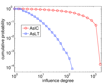
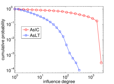
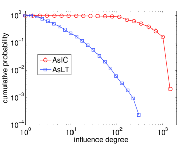
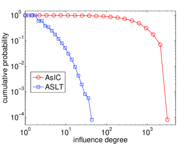
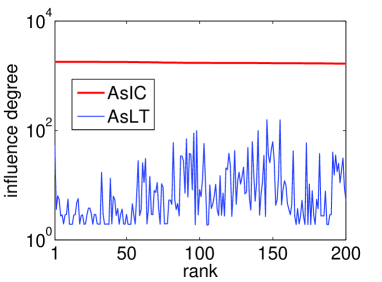
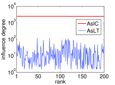
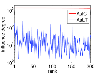
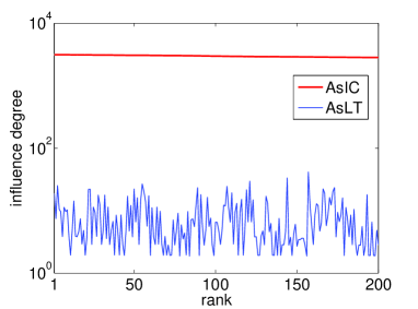
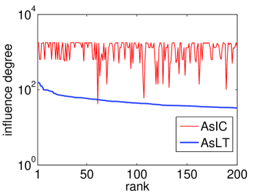
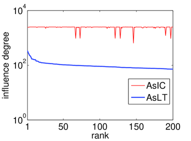
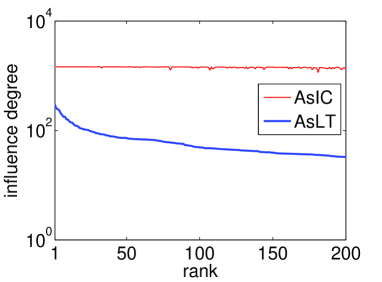
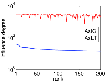
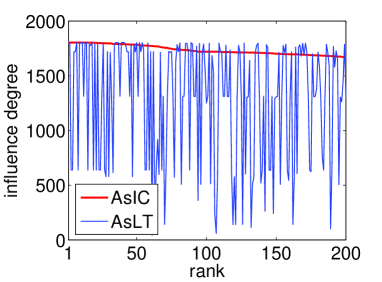
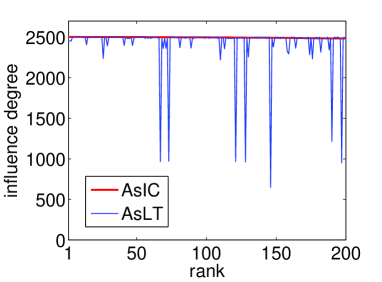
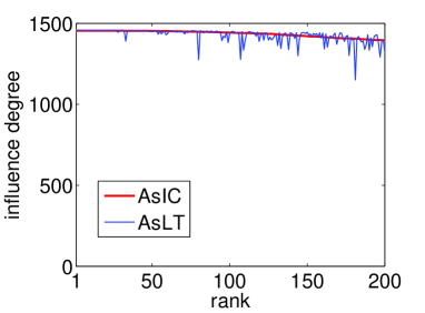
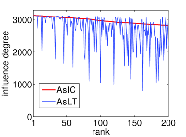
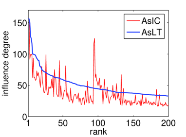
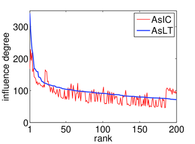
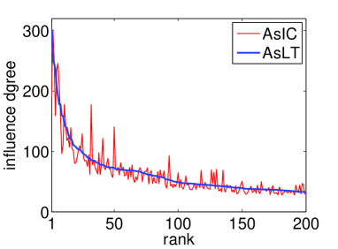
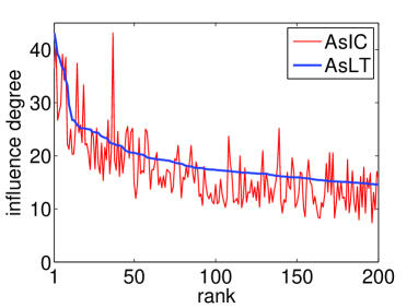
First, we investigated which of the AsIC and AsLT models can spread information more widely. Figure 1 shows the cumulative probability of influence degree, $f_{\sigma}(x)$ $=$ $|\{v\in V;\sigma(v)\geq x\}|/|V|$, for the AsIC and the AsLT models. At a glance we can see that the AsIC model has by far many more nodes of high influence degrees than the AsLT model. Further, we examined the difference of influence degree between the two models for the respective influential nodes of both the AsIC and the AsLT models. We ranked nodes according to the influence degree of AsIC and AsLT, respectively, and extracted the top $200$ influential nodes for each. Figures 2 and 3 display the respective influence degree of rank $k$ node of AsIC and AsLT ($k=1,\cdots,200$). Here, the red line indicates the influence degree of AsIC, and the blue line indicates the influence degree of AsLT. We can see that the difference of influence degree between the two models is quite large for these influential nodes. This clearly indicates that the information can diffuse more widely under the AsIC model than the AsLT model. This can be attributed to the scale-free nature (having power-law degree distributions) of the four real networks used in the experiments. It is known (?) that hub nodes, defined as those having many outgoing links, play an important role for widely spreading information in a scale-free network. By the information diffusion mechanism of the AsIC and AsLT models, it is more difficult for the AsLT model to transmit information to hub nodes than the AsIC model in a scale-free network. Therefore, the result is understandable.

Next, we compared the difference of the influential nodes between the AsIC and the AsLT models. The results are shown in Figures 4 and 5. For both figures the horizontal axes are node ranking ($k=1,\cdots,200$), and the actual ranking depends which model we are considering, e.g., the rank $k$ node for AsIC is different from the same rank $k$ node for AsLT. The vertical axis are influence degree for both figures, but it is the influence degree for AsIC in Figure 4 and that for AsLT in Figure 5. The red line corresponds to nodes for AsIC and the blue line corresponds to nodes for AsLT. Thus, by definition of node ranking, the influence degree of AsIC (red thick line) is non-increasing in Figure 4 and the influence degree of AsLT (blue thick line) in Figure 5 is non-increasing. However, the corresponding line for AsLT (blue line) in Figure 4 and that for AsIC (red line) in Figure 5 are very irregular. This means that almost all the nodes that are influential for AsIC model are different from the nodes that are influential for AsLT, and vice versa. There are small number of influential nodes that overlap for both the models, but how similar the influential nodes are (degree of overlapping) depends on the characteristics of the network structure, and no general tendency can be extracted.

5 Learning Performance Evaluation

5.1 Data Sets and Parameter Setting

We used the same four datasets that are used in Section 4, and employed also the simplest approximation for the parameter setting but with a slight difference according to the work ? (?).

We set $p_{u,v}=p$, $r_{u,v}=r$ for AsIC and $q_{u,v}=q|B(v)|^{-1}$, $r_{u,v}=r$ for AsLT. Under this assumption there is no need for the observation sequence data to pass through every link or node at minimum once and desirably several times. This drastically reduces the amount of data we have to generate to use as the training data to learn the parameters. Then, our task is to estimate the values of these parameters from the training data. According to the work of ? (?), we set $p$ to a value slightly smaller than $1/{\bar{d}}$. Thus, the true value of $p$ was set to $0.2$ for the coauthorship network, $0.1$ for the blog and Enron networks, and $0.02$ for the Wikipedia network. The true value of $q$ was set to $0.9$ for every network to achieve reasonably long diffusion results, and the true value of $r$ was set to $1.0$.

Using these parameter values, we generated a diffusion sequence from a randomly selected initial active node for each of the AsIC and the AsLT models in four networks. We then constructed a training dataset such that each diffusion sequence has at least 10 nodes. Parameter updating is terminated when either the iteration number reaches its maximum (set to 100) or the following condition is first satisfied: $|r^{(s+1)}-r^{(s)}|+|p^{(s+1)}-p^{(s)}|\leq 10^{-6}$ for AsIC and $|r^{(s+1)}-r^{(s)}|+|q^{(s+1)}-q^{(s)}|\leq 10^{-6}$ for AsLT, where the superscript $(s)$ indicates the value for the $s$-th iteration. In most of the cases, the above inequality is satisfied in less than 100 iterations. The converged values are rather insensitive to the initial parameter values, and we confirmed that the parameter updating algorithm stably converges to the correct values which we assumed to be the true values.

5.2 Parameter Estimation

Table 1: Parameter estimation error of the learning method for the AsIC model in four networks

Network	Number of active nodes	${\cal E}_{r}$	${\cal E}_{p}$
	1,163	0.019	0.026
Blog	5,151	0.018	0.014
	10,322	0.011	0.011
	1,275	0.060	0.032
Wikipedia	5,386	0.013	0.009
	10,543	0.006	0.007
	1,456	0.031	0.030
Enron	5,946	0.011	0.011
	10,468	0.005	0.006
	1,203	0.028	0.022
Coauthorship	5,193	0.009	0.007
	10,132	0.006	0.006

Table 2: Parameter estimation error of the learning method for the AsLT model in four networks

Network	Number of active nodes	${\cal E}_{r}$	${\cal E}_{q}$
	1,023	0.020	0.020
Blog	5,018	0.012	0.020
	10,037	0.012	0.020
	1018	0.032	0.024
Wikipedia	5,038	0.015	0.020
	10,025	0.006	0.017
	1,017	0.023	0.014
Enron	5,054	0.013	0.011
	10,024	0.007	0.010
	1,014	0.017	0.034
Coauthorship	5,023	0.017	0.029
	10,023	0.006	0.027

We generated the training set for each of the AsIC and the AsLT models as follows to evaluate the proposed learning methods as a function of the number of observed active nodes, i.e., amount of the training data. First we specified the target number $K$ of the active nodes we want to have, and the training set is generated by increasing the sequence one by one such that the total number of active nodes reaches $K$ with each sequence starting from a randomly chosen initial active node, skipping very short ones (those in which the number of nodes is less than 10). In the experiments, we investigated the cases of $K=1,000,5,000,10,000$. Let $r^{*}$, $p^{*}$ and $q^{*}$ denote the true values of $r$, $p$ and $q$, respectively, and $\hat{r}$, $\hat{p}$ and $\hat{q}$ the estimated values of $r$, $p$ and $q$, respectively. We define the parameter estimation errors ${\cal E}_{r}$, ${\cal E}_{p}$ and ${\cal E}_{q}$ by

$${\cal E}_{r}=\frac{|\hat{r}-r^{*}|}{r^{*}},\ \ \ {\cal E}_{p}=\frac{|\hat{p}-p^{*}|}{p^{*}},\ \ \ {\cal E}_{q}=\frac{|\hat{q}-q^{*}|}{q^{*}}.$$

Tables 1 and 2 show the parameter estimation errors of the proposed learning methods for the AsIC model and the AsLT model in four networks as a function of the number of observed active nodes, respectively. Here, the results are averaged over five independent experiments. As can be expected, the error is progressively reduced as the number of active nodes becomes larger. The algorithm guarantees to converge but does not guarantee the global optimal solution. In most of the cases, the number of iterations is less than 100. These results indicate that it converges to the correct solution in practice for all the parameters and for all the networks, which demonstrate the effectiveness of the proposed methods.

Table 3: Parameter estimation error of the learning method from a single observed sequence for four networks (Values in parentheses are standard deviations.)

Network		Blog	Wikipedia	Enron	Coauthorship
AsIC	${\cal E}_{r}$	0.091 (0.121)	0.088 (0.132)	0.029 (0.020)	0.119 (0.173)
	${\cal E}_{p}$	0.064 (0.085)	0.043 (0.056)	0.022 (0.019)	0.121 (0.255)
AsLT	${\cal E}_{r}$	0.188 (0.219)	0.192 (0.272)	0.143 (0.140)	0.214 (0.194)
	${\cal E}_{q}$	0.078 (0.049)	0.069 (0.043)	0.077 (0.053)	0.086 (0.054)

(a) Blog network

(b) Wikipedia network

(c) Enron network

(d) Coauthorship network

Figure 6: Influence curve and the learned parameter values from a single observed sequence in case of AsIC (There are 100 sequences and 100 points in each figure.)

(a) Blog network

(b) Wikipedia network

(c) Enron network

(d) Coauthorship network

Figure 7: Influence curve and the learned parameter values from a single observed sequence in case of AsLT (There are 100 sequences and 100 points in each figure.)

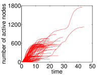
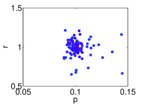
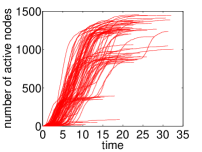
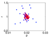
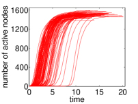
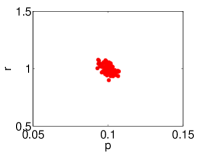
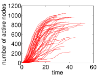
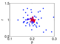
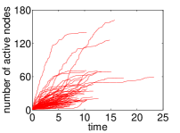
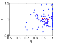
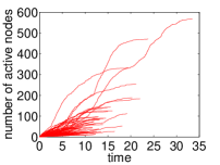
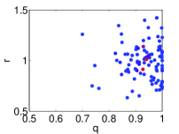
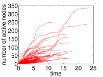
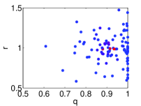
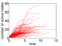
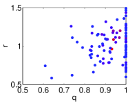
Next, we investigated the performance of the proposed learning method when the training set is a single diffusion sequence. Table 3 shows the results for four networks, where the results are averaged over $100$ independent experiments. Compared with Tables 1 and 2, the errors become larger. The average error of $p$ and $r$ for AsIC is 6% and 8%, and the average error of $q$ and $r$ for AsLT is 8% and 18%, respectively. The best results for AsIC is Enron network (2% for $p$ and 3% for $r$), and the best results for AsLT is Wikipedia network (7% for $q$) and Enron network (14% for $r$). The worst results for AsIC is Coauthorship network (12% for $p$ and 11% for $r$), and the worst results for AsLT is Coauthorship network (9% for $q$ and 21% for $r$). In general the accuracy is better for AsIC than for AsLT. This is because the lengths of the sequences are larger for AsIC. Further, $r$ is more difficult to correctly estimate than $p$ and $q$. In order to see the difference in the learning result for each sequence in more depth, we plotted the number of active nodes as a function of time (the influence curve), and the values of the parameters learned, $(p,r)$ for AsIC and $(q,r)$ for AsLT, in Figures 6 and 7. The length of each sequence varies considerably. Some sequences are short and some others are long. The color of the dots for the learned parameters is determined in such a way that it goes from true blue to true red in proportion to the sequence length, i.e., the shortest sequence is true blue and the longest sequence is true red. From these results we can see the algorithm learns the parameter values within 10% of the correct values if the length is reasonably long. For example, Enron network generates long sequences from all the randomly chosen initial active nodes in case of AsIC and the learning accuracy is very good. We draw a conclusion that although it is not desirable we can still estimate the parameter values from a single observation sequence if this is the only choice available.

5.3 Node Ranking

We measure the influence of node $v$ by the influence degree $\sigma(v)$ for the diffusion model that has generated ${\cal D}_{M}$. We compared the result of the high ranked influential nodes for the true model that uses the assumed true parameter values with 1) the proposed method that uses the learned parameter values, 2) four heuristics widely used in social network analysis (all computed by the network topology alone) and 3) the same proposed method in which an incorrect diffusion model is assumed, i.e., data generated by AsIC but learning assumed AsLT and vice versa. Here again the influence degree is estimated by the bond percolation method (?, ?), where we used $10,000$ bond percolation processes according to ? (?) and ? (?).

We call the proposed method the model based method. We call it the AsIC model based method if it employs the AsIC model as the information diffusion model. We then learn the parameters of the AsIC model from the observed data ${\cal D}_{M}$, and rank nodes according to the influence degrees based on the learned model. The AsLT model based method is defined in the same way. Among the four heuristics we used, the first three are “degree centrality”, “closeness centrality”, and “betweenness centrality”. These are commonly used as influence measure in sociology (?), where the out-degree of node $v$ is defined as the number of links going out from $v$, the closeness of node $v$ is defined as the reciprocal of the average distance between $v$ and other nodes in the network, and the betweenness of node $v$ is defined as the total number of shortest paths between pairs of nodes that pass through $v$. The fourth is “authoritativeness” obtained by the “PageRank” method (?). We considered this measure as one alternative since this is a well known method for identifying authoritative or influential pages in a hyperlink network of web pages. This method has a parameter $\varepsilon$; when we view it as a model of a random web surfer, $\varepsilon$ corresponds to the probability with which a surfer jumps to a page picked uniformly at random (?). In our experiments, we used a typical setting of $\varepsilon=0.15$.

(a) Blog network

(b) Wikipedia network

(c) Enron network

(d) Coauthorship network

Figure 8: Performance comparison in extracting influential nodes for the AsIC model

(a) Blog network

(b) Wikipedia network

(c) Enron network

(d) Coauthorship network

Figure 9: Performance comparison in extracting influential nodes for the AsLT model

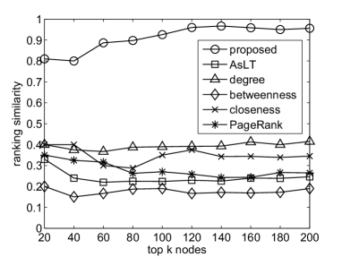
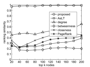
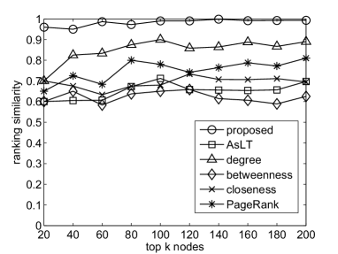
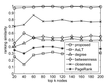
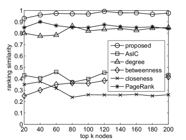
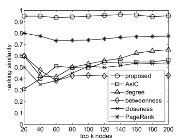
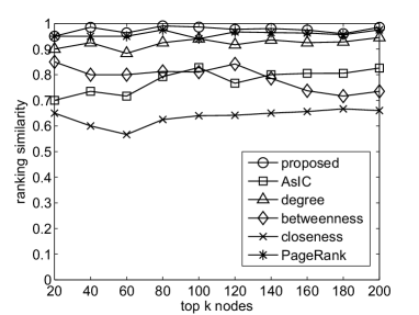
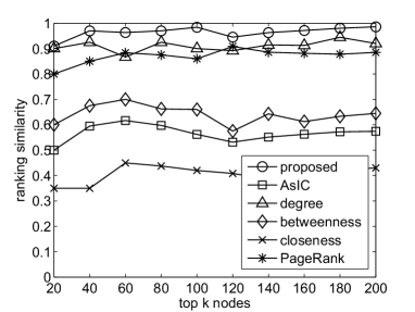
In terms of extracting influential nodes from the network $G=(V,E)$, we evaluated the performance of the ranking methods mentioned above by the ranking similarity ${\cal F}(k)={|L^{*}(k)\cap L(k)|}/{k}$ within the rank $k(>0)$, where $L^{*}(k)$ and $L(k)$ are the true set of top $k$ nodes and the set of top $k$ nodes for a given ranking method, respectively. We focused on the performance for high ranked nodes since we are interested in extracting influential nodes. Figures 8 and 9 show the results for the AsIC and the AsLT models, respectively. For the diffusion model based methods, we plotted the average value of ${\cal F}(k)$ at $k$ for five independent experimental results. We see that the proposed method gives better results than the other methods for these networks, demonstrating the effectiveness of our proposed learning method. It is interesting to note that the model based method in which an incorrect diffusion model is used is as bad as and in general worse than the heuristic methods. The results imply that it is important to consider the information diffusion process explicitly in discussing influential nodes and also to identify the correct model of information diffusion for the task in hand, same observation as in Section 4.

6 Model Selection

Now we have a method to estimate the parameter values from the observation for each of the assumed models. In this section we discuss whether the proposed learning method can correctly identify which of the two models: AsIC and AsLT the observed data come from, i.e., Model Selection problem. We assume that the topic is the decisive factor in determining the parameter values and place a constraint that the parameters depend only on topics but not on nodes and links of the network $G$, and differentiate different topics by assigning an index $l$ to topic $l$.

Therefore, we set $r_{l,u,v}=r_{l}$ and $p_{l,u,v}=p_{l}$ for any link $(u,v)\in E$ in case of the AsIC model and $r_{l,u,v}=r_{l}$ and $q_{l,u,v}=q_{l}|B(v)|^{-1}$ for any node $v\in V$ and link $(u,v)\in E$ in case of the AsLT model. Note that $0<q_{l}<1$ and $q_{v,v}=1-q_{l}$. Since we normally have a very small number of observation for each $(l,u,v)$, often only one, without this constraint, there is no way to learn the parameters.

6.1 Model Selection based on Predictive Accuracy

We have to select a model which is more appropriate to the model for the observed diffusion sequence. We decided to use predictive accuracy as the criterion for selection. We cannot use an information theoretic criterion such as AIC (Akaike Information Criterion)(?) or MDL (Minimum Description Length)(?) because we need to select the one from models with completely different probability distributions. Moreover, for both models, it is quite difficult to efficiently calculate the exact activation probability of each node for more than two information diffusion cascading steps ahead. In order to avoid these difficulties, we propose a method based on a hold-out strategy, which attempts to predict the activation probabilities at one step ahead and repeat this multiple times.

We now group the observed data sequences $D_{m}$ into topics. Assume that each topic $l$ has $M_{l}$ sequences of observation, i.e., $D_{l}=\{D_{l,m},\ m=1,\cdots,M_{l}\}$, where each $D_{l,m}$ is a set of pairs of active node and its activation time in the $m$-th diffusion result in the $l$-th topic. Accordingly we add a subscript $l$ to other variables, e.g., we denote $t_{l,m,v}$ to indicate the time $t$ that a node $v$ is activated in the $m$-th sequence of the $l$-th topic.

We learn the model parameters for each topic separately. This does not exclude treating each sequence in a topic separately and learn from each, i.e., $M_{l}=1$, which would help investigating if the same topic propagate similarly or not. For simplicity, we assume that for each $D_{l,m}$, the initial observation time $t_{l,m}$ is zero, i.e., $t_{l,m}=0$ for $m=1,\cdots,M_{l}$. Then, we introduce a set of observation periods

$${\cal I}_{l}=\{[0,\tau_{l,n});\ n=1,\cdots,N_{l}\},$$

where $N_{l}$ is the number of observation data we want to predict sequentially and each $\tau_{l,n}$ has the following property: There exists some $(v,t_{l,m,v})\in D_{l,m}$ such that $0<\tau_{l,n}<t_{l,m,v}$. Let $D_{l,m;\tau_{l,n}}$ denote the observation data in the period $[0,\tau_{l,n})$ for the $m$-th diffusion result in the $l$th topic, i.e.,

$$D_{l,m;\tau_{l,n}}=\{(v,t_{l,m,v})\in D_{l,m};\ t_{l,m,v}<\tau_{l,n}\}.$$

We also set ${\cal D}_{M_{l};\tau_{l,n}}$ $=$ $\{(D_{l,m;\tau_{l,n}},\tau_{l,n})$; $m$ $=$ $1$, $\cdots$, $M_{l}\}$. Let $\Theta$ denote the set of parameters for either the AsIC or the AsLT models, i.e., $\mbox{\boldmath$\Theta$}=(\mbox{\boldmath$r$},\mbox{\boldmath$p$})$ or $\mbox{\boldmath$\Theta$}=(\mbox{\boldmath$r$},\mbox{\boldmath$q$})$. We can estimate the values of $\Theta$ from the observation data ${\cal D}_{M_{l};\tau_{l,n}}$ by using the learning algorithms in Sections 3.1 (Appendix A.) and 3.2 (Appendix B.). Let $\widehat{\mbox{\boldmath$\Theta$}}_{\tau_{l,n}}$ denote the estimated values of $\Theta$. Then, we can calculate the activation probability $q_{\tau_{l,n}}(v,t)$ of node $v$ at time $t$ ($\geq\tau_{l,n}$) using $\widehat{\mbox{\boldmath$\Theta$}}_{\tau_{l,n}}$.

For each $\tau_{l,n}$, we select the node $v(\tau_{l,n})$ and the time $t_{l,m(\tau_{l,n}),v(\tau_{l,n})}$ by

$$t_{l,m(\tau_{l,n}),v(\tau_{l,n})}=\min\left\{t_{l,m,v};\ (v,t_{l,m,v})\in\bigcup_{m=1}^{M_{l}}(D_{l,m}\setminus D_{l,m;\tau_{l,n}})\right\}.$$

Note that $v(\tau_{l,n})$ is the first active node in $t\geq\tau_{l,n}$. We evaluate the predictive performance for the node $v(\tau_{l,n})$ at time $t_{l,m(\tau_{l,n}),v(\tau_{l,n})}$. Approximating the empirical distribution by

$$p_{\tau_{l,n}}(v,t)\ =\ \delta_{v,v(\tau_{l,n})}\ \delta(t-t_{l,m(\tau_{l,n}),v(\tau_{l,n})})$$

with respect to $(v(\tau_{n}),t_{l,m(\tau_{l,n}),v(\tau_{l,n})})$, we employ the Kullback-Leibler (KL) divergence

$$KL(p_{\tau_{l,n}}\,||\,q_{\tau_{l,n}})\ =\ -\sum_{v\in V}\int_{\tau_{l,n}}^{\infty}p_{\tau_{l,n}}(v,t)\log\frac{q_{\tau_{l,n}}(v,t)}{p_{\tau_{l,n}}(v,t)}\,dt,$$

where $\delta_{v,w}$ and $\delta(t)$ stand for Kronecker’s delta and Dirac’s delta function, respectively. Then, we can easily show

$$KL(p_{\tau_{l,n}}\,||\,q_{\tau_{l,n}})\ =\ -\log h_{m(\tau_{l,n}),v(\tau_{l,n})}.$$ (14)

By averaging the above KL divergence with respect to ${\cal I}_{l}$, we propose the following model selection criterion $\cal E$ (see Equation (14)):

$${\cal E}({\cal A};D_{l,1}\cup\cdots\cup D_{l,M_{l}}) = -\frac{1}{N_{l}}\sum_{n=1}^{N_{l}}\log h_{m(\tau_{l,n}),v(\tau_{l,n})},$$ (15)

where ${\cal A}$ expresses the information diffusion model (i.e., the AsIC or the AsLT models). In our experiments, we adopted

$${\cal I}_{l}\ =\ \{[0,t_{l,m,v});\ (v,t_{l,m,v})\in D_{l,1}\cup\cdots\cup D_{l,M_{l}},\ t_{l,m,v}\geq\tau_{0}\},$$

where $\tau_{0}$ is the median time of all the observed activation time points.

6.2 Evaluation by Synthetic Data

Our goal here is to evaluate the model selection method to see how accurately it can detect the true model that generated the data, using topological structure of four large real networks described in Section 4.1. We assumed the true model by which the data are generated to be either AsLT or AsIC. We have to repeatedly estimate the parameters using the proposed parameter update algorithms. In actual computation the learned values for observation period $[0,\tau_{l,n}]$ are used as the initial values for observation period $[0,\tau_{l,n+1}]$ for efficiency purpose.

The average KL divergence given by Equation (15) is the measure for the goodness of the model ${\cal A}$ for a training set $D_{l}$ of $M_{l}$ sequences with respect to topic $l$. The smaller its value is, the better the model explains the data in terms of predictability. Thus, we can estimate the true model from which $D_{l}$ is generated to be AsIC if ${\cal E}(AsIC;D_{l})<{\cal E}(AsLT;D_{l})$, and vice versa. Using each of the AsIC and the AsLT models as the true model, we generated a training set $D_{l}$. Here we set $M_{l}=1$, i.e., we generated a single diffusion sequence, learned a model and performed the model selection. We repeated this 100 times independently for the four networks mentioned before. We could have set $M_{l}=100$ and learned a single parameter set. This is more reliable, but we wanted to know whether the model selection algorithm works well or not using only a single sequence of data.

Table 4: Accuracy of the model selection method for four networks

Network	Blog	Wikipedia	Enron	Coauthorship
AsIC	92	100	100	93
	(370.2)	(920.8)	(1500.6)	(383.5)
AsLT	79	86	99	76
	(28.2)	(54.0)	(47.7)	(19.0)

(a) Blog network

(b) Wikipedia network

(c) Enron network

(d) Coauthorship network

Figure 10: Relation between the length of sequence and the accuracy of model selection for a single diffusion sequence generated from the AsIC model (There are 100 points.)

(a) Blog network

(b) Wikipedia network

(c) Enron network

(d) Coauthorship network

Figure 11: Relation between the length of sequence and the accuracy of model selection for a single diffusion sequence generated from the AsLT model (There are 100 points.)

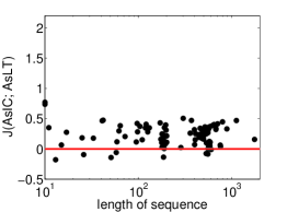
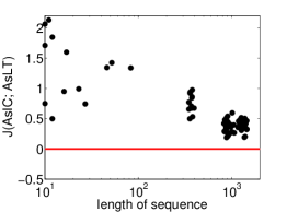
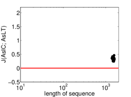
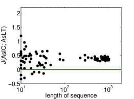
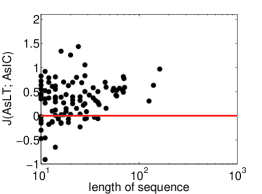
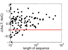
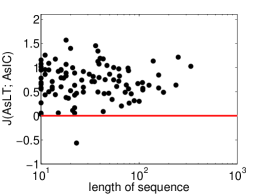
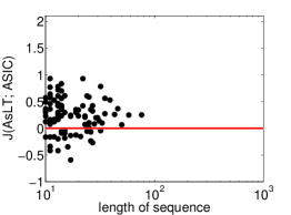
Table 4 summarizes the number of times that the model selection method correctly identified the true model. The number within the parentheses is the average length of the diffusion sequences in the training set. From these results, we can say that the proposed method achieved a good accuracy, 90.6% on average. Especially, for the Enron network, its estimation was almost perfect. To analyze the performance of the proposed method more deeply, we investigated the relation between the length of sequence and the model selection result. Figure 10 shows the results for the case that $D_{l}$ is generated by the AsIC model. Here, the horizontal axis denotes the length of sequence in each dataset and the vertical axis is the difference of the average KL divergence defined by $J(AsIC;AsLT)={\cal E}(AsLT;D_{l})-{\cal E}(AsIC;D_{l})$. Thus, $J(AsIC;AsLT)>0$ means that the proposed method correctly estimated the true model AsIC because it means

${\cal E}(AsIC;D_{l})$ is smaller than ${\cal E}(AsLT;D_{l})$. From the figure, we can see that there is a correlation between the length of sequence and the estimation accuracy, and that the misselection occurs when the length of the sequence is short. In particular, Wikipedia and Blog networks have no misselection. Figure 11 shows the results for the case that $D_{l}$ is generated by the AsLT model. Here, $J(AsLT;AsIC)={\cal E}(AsIC;D_{l})-{\cal E}(AsLT;D_{l})$. We notice that the overall accuracy becomes 95.5% when considering only the sequences that contain no less than 20 nodes. This means that the proposed model selection method is highly reliable for a long sequence and its accuracy could asymptotically approach to 100% as the sequence gets longer. We can also see from Figures 10 and 11 that the results for the AsIC model are better than those for the AsLT model. We note that the plots for the diffusion sequences generated from the AsIC model are shifted to the right in all networks, meaning that the diffusion sequences are longer for AsIC than for AsLT. The better accuracy is attributed to this.

6.3 Evaluation by Real World Blog Data

We analyzed the behavior of topics in a real world blog data. Here, again, we assumed the true model behind the data to be either the AsIC model or the AsLT model. Using each pair of the estimated parameters, $(r_{l},p_{l})$ for AsIC and $(r_{l},q_{l})$ for AsLT, we first analyzed the behavior of people with respect to the information topics by simply plotting them as a point in $2$-dimensional space. We next estimated the true model for each topic by applying the model selection method described in Section 6.1.

6.3.1 Data Sets and Parameter Setting

We employed the real blogroll network used by ? (?), which was generated from the database of a blog-hosting service in Japan called Doblog. In the network, bloggers are connected to each other and we assume that topics propagate from blogger $x$ to another blogger $y$ when there is a blogroll link from $y$ to $x$. In addition, according to the work of ? (?), it is assumed that a topic is represented as a URL which can be tracked down from blog to blog. We used the propagation sequences of 172 URLs for this analysis, each of which has at least 10 time steps. In these 172 URLs some of them are the same, meaning that there are multiple sequences for the same topic, i.e., $M_{l}>1$. However, as in the analysis of Section 6.2, we treated them as if $M_{l}=1$ and used each sequence independently. The main reason for this is that we want to investigate whether the same topic propagates in the same way when there are multiple sequences as well as to test whether the model selection is feasible from a single sequence data in case of the real data.

(a) The AsIC model based method

(b) The AsLT model based method

Figure 12: Results for the Doblog database

6.3.2 Parameter Estimation

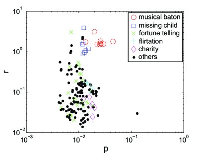
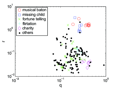
We ran the experiments for each identified URL and obtained the parameters $p$ and $r$ for the AsIC model based method and $q$ and $r$ for the AsLT model based method. Figures 12a and 12b are the plots of the results for the major URLs (topics) by the AsIC and AsLT methods, respectively. The horizontal axis is the diffusion parameter $p$ for the AsIC method and $q$ for the AsLT method, while the vertical axis is the delay parameter $r$ for both. The latter axis is normalized such that $r=1$ corresponds to a delay of one day, meaning $r=0.1$ corresponds to a delay of 10 days. In these figures, we used five kinds of markers other than dots, to represent five different typical URLs: the circle ($\circ$) stands for a URL that corresponds to the musical baton which is a kind of telephone game on the Internet (the musical baton), the square ($\Box$) for a URL that corresponds to articles about a missing child (the missing child), the cross ($\times$) for a URL that corresponds to articles about fortune telling (the fortune telling), the diamond ($\Diamond$) for a URL of a certain charity site (the charity), and the plus ($+$) for a URL of a site for flirtatious tendency test (the flirtation). All the other topics are denoted by dots ($\cdot$), which means they are a mixture of many topics.

The results indicate that in general both the AsIC and AsLT models capture reasonably well the characteristic properties of topics in a similar way. We note that the same topic behaves similarly for different sequences except for the fortune telling. This supports the assumption we made in Section 6.1. Careful look at the URLs used to identify the topic of fortune telling indicates that there are multiple URLs involved and mixing them as a single topic may have been a too crude assumption. Other interpretation is that people’s perception on this topic is not uniform and varies considerably from person to person and should be viewed as an exception of the assumption. Behavior of the other topics is interpretable. For example, the results capture the urgency of the missing child, which propagates quickly with a meaningful probability (one out of 80 persons responds). Musical baton which actually became the latest craze on the Internet also propagates quickly (less than one day on the average) with a good chance (one out of 25 to 100 persons responds). In contrast non-emergency topics such as the flirtation and the charity propagate very slowly. We further note that the dependency of topics on the parameter $r$ is almost the same for both AsIC and AsLT, but that on the parameters $p$ and $q$ is slightly different, e.g., relative difference of musical baton, missing child and charity. Although $p$ and $q$ are different parameters but both are the measures that represent how easily the diffusion takes place. As is shown in Section 5.3, the influential nodes are very sensitive to the model used and this can be attributed to the differences of these parameter values.

6.3.3 Results of Model Selection

Table 5: Results of model selection for the Doblog dataset

Topic	Total	AsLT	AsIC
Musical baton	9	5	4
Missing child	7	0	7
Fortune telling	28	4	24
Charity	6	5	1
Flirtation	7	7	0
Others	115	11	104

Figure 13: The relation between the KL difference and sequence length for the Doblog database

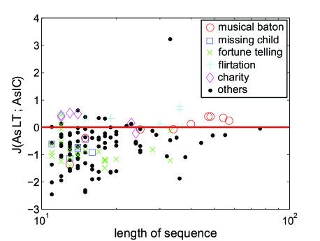
In the analysis of previous subsection, we assumed that all topics follow the same diffusion model. However, in reality this is not true and each topic should propagate following more closely to either one of the AsLT and AsIC models. We attempt to estimate the underlying behavior model of each topic by applying the model selection method described in Section 6.1. As explained, we treat each sequence independently and learn the parameters from each sequence, calculate its KL divergences by Equation (15) for both the models, and compare the goodness. Table 5 and Figure 13 summarize the results. From these results, we can see that most of the diffusion behaviors on this blog network follow the AsIC model. It is interesting to note that the model estimated for the musical baton is not identical to that for the missing child although their diffusion patterns are very similar (see Section 6.3.2). The missing child strictly follows the AsIC model. This is attributed to its greater urgency. People would post what they know if they think it is useful without influenced by the behaviors of their neighbors. For musical baton Table 5 indicates that the numbers are almost tie (4 vs. 5), but we saw in Section 6.2 that the longer sequence gives a better accuracy, and the models selected in longer sequences are all AsLT in Figure 13 for musical baton. Thus, we estimate that musical baton follows more closely to AsLT. This can be interpreted that people follow their friends in this game. Likewise, it is easy to imagine that people would behave similarly to their neighbors when requested to give a donation. This explains that charity follows AsLT. The flirtation clearly follows AsLT. People are attempted to do bad things when their neighbor do so. Note that there exists one dot at near the top center in Figure 13, showing the greatest tendency to follow AsLT. This dot represents a typical circle site that distributes one’s original news article on personal events.

7 Discussion

? (?) have recently proposed a method in which the liklihood is described in somewhat generic way with respect to a given diffusion dataset for a wide class of IC type information diffusion models. Their purpose is to infer the latent network structure. On the other hand, our interest is to explore the salient characteristics of two contrasting information diffusion models assuming that the structure is known. Although their purpose is substantially different from ours, we share with them the common idea of estimating parameters in information diffusion models. However, there exist some mathematically notable differences. The main difference comes from the derivation of the probability density $h_{m,v}$ that one or more active parent nodes of a node $v$ succeed(s) in activating $v$ at time $t_{m,v}$ for the $m$-diffusion sequence (see Equation (4)). In order to clarify this point, we denote the corresponding formula used in ? (?) by $\tilde{h}_{m,v}$, then $\tilde{h}_{m,v}$ is expressed as follows:

$$\tilde{h}_{m,v} = 1-\prod_{u\in C_{m}(t_{m,v})}(1-w(t_{m,v}-t_{m,u})A_{i,j}).$$ (16)

where, according to their terminology, $w(t)$ and $A_{i,j}$ stand for the transmission time model and the conditional probability of infection transmission, respectively. Here note that the product term $w(t_{m,v}-t_{m,u})A_{i,j}$ is equivalent to our formula ${\cal X}_{m,u,v}$, where ${\cal X}_{m,u,v}$ is defined as the probability density that a node $u$ activates the node $v$ at time $t_{m,v}$. (see Equation (2)).

For an active parent node $u$, the term $(1-w(t_{m,v}-t_{m,u})A_{i,j})$ appearing in Equation (16) conceptually corresponds to our formula ${\cal Y}_{m,u,v}$, where ${\cal Y}_{m,u,v}$ is defined as the probability that the node $v$ is not activated by the node $u$ within the time-period $[t_{m,u},t_{m,v})$ (see Equation (3)). Here note that from the observed $m$-th diffusion sequence, we know for sure that the node $u$ could not succeed in activating $v$ during the time interval $t\in[t_{m,u},t_{m,v})$. Namely, our formulation reflects this observation explicitly in probability estimation, rather than just subtracting the probability from $1$, as in the expression $(1-w(t_{m,v}-t_{m,u})A_{i,j})$. Furthermore, we can transform Equation (3) as follows:

$${\cal Y}_{m,u,v} = (1-p_{u,v})+\int_{t_{m,v}}^{\infty}p_{u,v}r_{u,v}\exp(-r_{u,v}(t-t_{m,u}))~{}dt.$$ (17)

Here we can naturally interpret this formula as follows: the first term of right-hand-side is the probability that the node $u$ fails to activate $v$, and the second term corresponds to the probability that the node $u$ succeeds in activating $v$ after the $t_{m,v}$, i.e., the fact that the node $v$ is not activated by the node $u$ within the time-period $[t_{m,u},t_{m,v})$ means that it has either failed to activate $v$ at all or succeeded to activate $v$ but the activation time is outside of the observed time-period. The basic interpretation of $\tilde{h}_{m,v}$ is that at least one active parent node activates $v$ at time $t_{m,v}$. Namely, the formulation allows that $v$ is activated simultaneously by its multiple parent nodes exactly at time $t_{m,v}$, while our formulation does not consider this possibility. When the diffusion process unfolds in continuous-time $t$, the probability measure of such simultaneous activation is zero. Thus, we employ our $h_{m,v}$ formulation as described in Equation (4)). Of course, in case of the discrete-time modeling, the situation of simultaneous activation by multiple active parents must be considered adequately. The objective function for this case under the discrete-time IC model has been derived in ? (?). The major advantage of their method is that it guarantees a unique optimal solution, whereas ours only guarantees that it converges to a stationary solution which is not necessarily a global maximum. However, it is not clear that a similar approach can be applied to Linear Threshold type diffusion models. In addition, as discussed above and also shown in Section 3.3, we need to elaborate on the formula for $h_{m,v}$ in order to model the information diffusion process more accurately reflecting subtle notion of different time delay models and as much information of observed data as possible. It is also not clear that the above advantage of their formulation still holds when the formula for $\tilde{h}_{m,v}$ is modified accordingly. Our view is that their formulation can be a useful technique for inferring latent network structure, but it has limitation if we use it to explore the salient characteristics of different diffusion models. In this sense, we believe that our approach based on the EM-like learning algorithm remains vital and useful for a wide class of information diffusion models.

We started with general description for the parameter values but had to introduce drastic simplification in experimental evaluations both for synthetic datasets and real world datasets. The results in Section 6.3.2 implies that the assumption of topics being a decisive factor for diffusion parameter values seems to be plausible, which in turn justifies the use of the same parameter values for multiple sequence observation data if they are talking on the same topic. However, as one counter example is observed (fortune telling), this is definitely not true in general. Finding a small number of factors, e.g., important node attributes, from which the parameter values can be estimated in good accuracy is a crucial problem. Learning such dependency is easy as exemplified in ? (?) once such factors are identified and the real world data for such factors ara available as part of observed information diffusion data.

As we explained in Section 5.3, the ranking results that involve detailed probabilistic simulation are very sensitive to the underlying model which is assumed to generate the observed data. In other words, it is very important to select an appropriate model for the analysis of information diffusion from which the data has been generated if the node characteristics are the main objective of analysis, e.g., such problems as the influence maximization problem  (?, ?), a problem at a more detailed level. However, it is also true that the parameters for the topics that actually propagated quickly/slowly in observation converged to the values that enable them to propagate quickly/slowly on the model, regardless of the model chosen. Namely, we can say that the difference of models does not have much influence on the relative difference of topic propagation which indeed strongly depends on topic itself. Both models are well defined and can explain this property at this level of abstraction. Nevertheless, the model selection is very important if we want to characterize how each topic propagates through the network.

One of the objectives of this paper is to understand the behavioral difference between the AsIC model and the AsLT model. The analysis in Section 4.2 is based on the network structures taken from real world data. We feel more mathematical-oriented treatment is needed to qualitatively understand the behavior difference of these two models for a wide class of graphs from various perspectives, e.g., types of graphs: regular vs random, graphs with different characteristics: power-law, small-worldness, community structure, etc.

There are other studies that deal with topic dependent information diffusion. Recent study by ? (?) discusses differences in the diffusion mechanism across different topics. They experimentally obtain from the observation data the probability $p(k)$ that a node gets activated after its active parents failed to activate it $k-1$ times in succession, and model the diffusion process using $p(k)$ under the SIR (Susceptible/Infectious/Recover) setting. Their finding is that the shape of $p(k)$ differs considerably from one topic to another, which is characterized by two factors, stickness (maximum value of $p(k)$) and persistency (rate of $p(k)$’s decay after the peak), and that the repeated exposures to a topic are particularly crucial when it is in some way controversial or contentious. Another recent study on Twitter by ? (?) attempts to quantify a node’s influence degree (the number of nodes that a seed node (initial node) can activate by learning a regression tree using various node’s attributes such as no. of followers, no. of friends, no. of tweets, past influence degree and content related features. To their surprise none of the content related attributes are selected in the learned regression tree. They attribute this to the fact that most explanations of success tend to focus only on observed success, which invariably represent a small and biased sample of the total population. They conclude that individual level predictions of influence is unreliable, and it is important to rely on average performance. Both studies approach the similar problem from different angles. There are many factors that need be considered and much more work is needed to understand this problem.

8 Conclusion

We deal with the problem of analyzing information diffusion process in a social network using probabilistic information diffusion models. There are two contrasting fundamental models that have been widely used by many people: Independent Cascade model and Linear Threshold model. These are modeled based on two different ends of the spectrum. The IC model is sender-centered (information push style model) where the information sender tries to push information to its neighbors, whereas the LT model is receiver-centered (information pull style model where the information receiver tries to pull information. We extended these two contrasting models (called AsIC and AsLT) by incorporating asynchronous time delay to make them realistic enabling effective use of observed information diffusion data. Using these as the basic tools, we challenged the following three problems: 1) to clarify how these two contrasting models differ from or similar to each other in terms of information diffusion, 2) to devise effective algorithms to learn the model itself from the observed information diffusion data, and 3) to identify which model is more appropriate to explain for a particular topic (information) to diffuse/propagate.

We first showed that there can be variations to each of these two models depending on how we treat time delay. We identified there are two kinds of time delay: link delay and node delay, and the latter is further divided into two categories: override and non-override. We derived the liklihood function, the probability density to generate the observed data for each model. Choosing one particular time delay model, we showed that the model parameters are learnable from a limited amount of observation by deriving the parameter update algorithm for both AsIC and AsLT that maximizes the likelihood function which is guaranteed to converge and performs stably. We also proposed a method to select a model that better explains the observation based on its predictive accuracy. To this end, we devised a variant of hold-out training algorithm applicable to a set of sequential data and a method to select a better model by comparing the predictive accuracy using the KL divergence.

Extensive evaluations were performed using both synthetic data and real data. We first showed using synthetic data with the network structures taken from four real networks that there are considerable behavioral difference between the AsIC and the AsLT models, and gave a qualitative account of why such difference is brought. We then experimentally confirmed that the proposed parameter update algorithm converges to the correct values very stably and efficiently, it can learn the parameter values even from a single observation sequence if its length is reasonably long, it can estimate the influential nodes quite accurately whereas the frequently used centrality heuristics performs very poorly, the influential nodes are very sensitive to the model used, and the proposed model selection method can correctly identify the diffusion models by which the observed data is generated. We further applied the methods to the real blog data and analyzed the behavior of topic propagation. The relative propagation speed of topics, i.e., how far/near and how fast/slow each topic propagates, that are derived from the learned parameter values is rather insensitive to the model selected, but the model selection algorithm clearly identifies the difference of model goodness for each topic. We found that many of the topics follow the AsIC model in general, but some specific topics have clear interpretations for them being better modeled by either one of the two, and these interpretations are consistent with the model selection results. There are numerous factors that affect the information diffusion process, and there can be a number of different models. Understanding the behavioral difference of each model, learning these models efficiently from the available data and selecting the correct model are a big challenge in social network analysis and this work is the first step towards this goal.

Acknowledgments

This work was partly supported by Asian Office of Aerospace Research and Development, Air Force Office of Scientific Research under Grant No. AOARD-11-4111, and JSPS Grant-in-Aid for Scientific Research (C) (No. 23500194).

Appendix A. Learning Algorithm for AsIC model

Maximizing ${\cal L}(\mbox{\boldmath$r$},\mbox{\boldmath$p$};{\cal D}_{M})$ is equivalent to maximizing its logarithm. Let $\bar{\mbox{\boldmath$r$}}=({\bar{r}}_{u,v})$ and $\bar{\mbox{\boldmath$p$}}=({\bar{p}}_{u,v})$ be the current estimates of $r$ and $p$, respectively. Taking $\log$ of $h_{m,v}$ involves $\log$ of sum of ${\cal X}_{m,u,v}({\cal Y}_{m,u,v})^{-1}$, which is problematic. To get around this problem, we define $\alpha_{m,u,v}$ for each $(v,t_{m,v})\in D_{m}$ and $u$ $\in$ ${\cal B}_{m,v}$, by

$$\alpha_{m,u,v}\ =\ {\cal X}_{m,u,v}({\cal Y}_{m,u,v})^{-1}\,\left/\,\sum_{z\in{\cal B}_{m,v}}{\cal X}_{m,z,v}({\cal Y}_{m,z,v})^{-1}.\right.$$

Let $\bar{\cal X}_{m,u,v}$, $\bar{\cal Y}_{m,u,v}$, $\bar{h}_{m,v}$, and $\bar{\alpha}_{m,u,v}$ denote the values of ${\cal X}_{m,u,v}$, ${\cal Y}_{m,u,v}$, $h_{m,v}$, and $\alpha_{m,u,v}$ calculated by using $\bar{\mbox{\boldmath$r$}}$ and $\bar{\mbox{\boldmath$p$}}$, respectively.

From Equations (4), (6) and (8), we can transform our objective function ${\cal L}(\mbox{\boldmath$r$},\mbox{\boldmath$p$};{\cal D}_{M})$ as follows:

$$\log{\cal L}(\mbox{\boldmath$r$},\mbox{\boldmath$p$};{\cal D}_{M})=Q(\mbox{\boldmath$r$},\mbox{\boldmath$p$};\bar{\mbox{\boldmath$r$}},\bar{\mbox{\boldmath$p$}})-H(\mbox{\boldmath$r$},\mbox{\boldmath$p$};\bar{\mbox{\boldmath$r$}},\bar{\mbox{\boldmath$p$}}),$$ (18)

where $Q(\mbox{\boldmath$r$},\mbox{\boldmath$p$};\bar{\mbox{\boldmath$r$}},\bar{\mbox{\boldmath$p$}})$ is defined by

$$Q(\mbox{\boldmath$r$},\mbox{\boldmath$p$};\bar{\mbox{\boldmath$r$}},\bar{\mbox{\boldmath$p$}})=\sum_{m=1}^{M}\left(\sum_{v\in C_{m}}Q_{m,v}+\sum_{v\in C_{m}}\sum_{w\in F(v)\setminus C_{m}}\log(1-p_{v,w})\right),$$

$$Q_{m,v}=\sum_{u\in{\cal B}_{m,v}}\log\left({\cal Y}_{m,u,v}\right)+\sum_{u\in{\cal B}_{m,v}}{\bar{\alpha}}_{m,u,v}\log\left({\cal X}_{m,u,v}({\cal Y}_{m,u,v})^{-1}\right)$$

and $H(\mbox{\boldmath$r$},\mbox{\boldmath$p$};\bar{\mbox{\boldmath$r$}},\bar{\mbox{\boldmath$p$}})$ is defined by

$$H(\mbox{\boldmath$r$},\mbox{\boldmath$p$};\bar{\mbox{\boldmath$r$}},\bar{\mbox{\boldmath$p$}})=\sum_{m=1}^{M}\sum_{v\in C_{m}}\sum_{u\in{\cal B}_{m,v}}{\bar{\alpha}}_{m,u,v}\log\alpha_{m,u,v}.$$ (19)

Since $H(\mbox{\boldmath$r$},\mbox{\boldmath$p$};\bar{\mbox{\boldmath$r$}},\bar{\mbox{\boldmath$p$}})$ is maximized at $\mbox{\boldmath$r$}=\bar{\mbox{\boldmath$r$}}$ and $\mbox{\boldmath$p$}=\bar{\mbox{\boldmath$p$}}$ from Equation (19), we can increase the value of ${\cal L}(\mbox{\boldmath$r$},\mbox{\boldmath$p$};{\cal D}_{M})$ by maximizing $Q(\mbox{\boldmath$r$},\mbox{\boldmath$p$};\bar{\mbox{\boldmath$r$}},\bar{\mbox{\boldmath$p$}})$ (see Equation (18)). Note here that $Q$ is a convex function with respect to $r$ and $p$, and thus the convergence is guaranteed. Here again we have a problem of $\log$ of sum for $\log{\cal Y}_{m,u,v}$. In order to cope with this problem, we transform $\log{\cal Y}_{m,u,v}$ in the same way as we introduced $\alpha_{m,u,v}$, and define $\beta_{m,u,v}$ by

$$\beta_{m,u,v}=p_{u,v}\exp(-r_{u,v}(t_{m,v}-t_{m,u}))\,/\,{\cal Y}_{m,u,v}.$$

Finally, we obtain the following update formulas of our estimation method as the solution which maximizes $Q(\mbox{\boldmath$r$},\mbox{\boldmath$p$};\bar{\mbox{\boldmath$r$}},\bar{\mbox{\boldmath$p$}})$:

$$r_{u,v} = \frac{\sum_{m\in{\cal M}^{+}_{u,v}}\bar{\alpha}_{m,u,v}}{\sum_{m\in{\cal M}^{+}_{u,v}}(\bar{\alpha}_{m,u,v}+(1-\bar{\alpha}_{m,u,v})\bar{\beta}_{m,u,v})(t_{m,v}-t_{m,u})},$$

$$p_{u,v} = \frac{1}{|{\cal M}^{+}_{u,v}|+|{\cal M}^{-}_{u,v}|}\sum_{m\in{\cal M}^{+}_{u,v}}(\bar{\alpha}_{m,u,v}+(1-\bar{\alpha}_{m,u,v})\bar{\beta}_{m,u,v}),$$

where ${\cal M}^{+}_{u,v}$ and ${\cal M}^{-}_{u,v}$ are defined by

$${\cal M}^{+}_{u,v} = \{m\in\{1,\cdots,M\};\ v\in C_{m},\ u\in{\cal B}_{m,v}\},$$

$${\cal M}^{-}_{u,v} = \{m\in\{1,\cdots,M\};\ u\in C_{m},\ v\in\partial C_{m}\}.$$

Note that we can regard our estimation method as a variant of the EM algorithm. We want to emphasize here that each time iteration proceeds the value of the likelihood function never decreases and the iterative algorithm is guaranteed to converge due to the convexity of $Q$.

Appendix B. Learning Algorithm for AsLT model

An iterative parameter update algorithm similar to the AsIC model can be derived for the AsLT model, too. We first define $\phi_{m,u,v}$ for each $v\in C_{m}$ and $u\in{\cal B}_{m,v}$, $\varphi_{m,u,v}$ for each $v\in\partial C_{m}$ and $u$ $\in$ $\{v\}$ $\cup$ $B(v)$ $\setminus$ ${\cal B}_{m,v}$, and $\psi_{m,u,v}$ for each $v\in\partial C_{m}$ and $u\in{\cal B}_{m,v}$, respectively by the following formulas.

$$\phi_{m,u,v} = q_{u,v}r_{u,v}\exp(-r_{u,v}(t_{m,v}-t_{m,u}))\,/\,h_{m,v},$$

$$\varphi_{m,u,v} = q_{u,v}\,/\,g_{m,v},$$

$$\psi_{m,u,v} = q_{u,v}\exp(-r_{u,v}(T_{m}-t_{m,u}))\,/\,g_{m,v}.$$

Let $\bar{\mbox{\boldmath$r$}}=({\bar{r}}_{v})$ and $\bar{\mbox{\boldmath$q$}}=({\bar{q}}_{u,v})$ be the current estimates of $r$ and $q$, respectively. Similarly, let $\bar{\phi}_{m,u,v}$, $\bar{\varphi}_{m,u,v}$, and $\bar{\psi}_{m,u,v}$ denote the values of ${\phi}_{m,u,v}$, ${\varphi}_{m,u,v}$, and ${\psi}_{m,u,v}$ calculated by using $\bar{\mbox{\boldmath$r$}}$ and $\bar{\mbox{\boldmath$q$}}$, respectively.

From Equations (10), (11) and (12), we can transform ${\cal L}(\mbox{\boldmath$r$},\mbox{\boldmath$q$};{\cal D}_{M})$ as follows:

$$\log{\cal L}(\mbox{\boldmath$r$},\mbox{\boldmath$q$};{\cal D}_{M})=Q(\mbox{\boldmath$r$},\mbox{\boldmath$q$};\bar{\mbox{\boldmath$r$}},\bar{\mbox{\boldmath$q$}})-H(\mbox{\boldmath$r$},\mbox{\boldmath$q$};\bar{\mbox{\boldmath$r$}},\bar{\mbox{\boldmath$q$}}),$$ (20)

where $Q(\mbox{\boldmath$r$},\mbox{\boldmath$q$};\bar{\mbox{\boldmath$r$}},\bar{\mbox{\boldmath$q$}})$ is defined by

$$Q(\mbox{\boldmath$r$},\mbox{\boldmath$q$};\bar{\mbox{\boldmath$r$}},\bar{\mbox{\boldmath$q$}})=\sum_{m=1}^{M}\left(\sum_{v\in C_{m}}Q_{m,v}^{(1)}+\sum_{v\in\partial C_{m}}Q_{m,v}^{(2)}\right),$$ (21)

$$Q_{m,v}^{(1)} = \sum_{u\in{\cal B}_{m,v}}\bar{\phi}_{m,u,v}\log(q_{u,v}r_{v}\exp(-r_{v}(t_{m,v}-t_{m,u})))$$

$$Q_{m,v}^{(2)} = \sum_{u\in\{v\}\cup B(v)\setminus{\cal B}_{m,v}}\bar{\varphi}_{m,u,v}\log(q_{u,v})+\sum_{u\in{\cal B}_{m,v}}\bar{\psi}_{m,u,v}\log(q_{u,v}\exp(-r_{v}(T_{m}-t_{m,u}))).$$

It is easy to see that $Q(\mbox{\boldmath$r$},\mbox{\boldmath$q$};\bar{\mbox{\boldmath$r$}},\bar{\mbox{\boldmath$q$}})$ is convex with respect to $r$ and $q$, and $H(\mbox{\boldmath$r$},\mbox{\boldmath$p$};\bar{\mbox{\boldmath$r$}},\bar{\mbox{\boldmath$q$}})$ is defined by

$$H(\mbox{\boldmath$r$},\mbox{\boldmath$q$};\bar{\mbox{\boldmath$r$}},\bar{\mbox{\boldmath$q$}})=\sum_{m=1}^{M}\left(\sum_{v\in C_{m}}H_{m,v}^{(1)}+\sum_{v\in\partial C_{m}}H_{m,v}^{(2)}\right),$$ (22)

$$H_{m,v}^{(1)} = \sum_{u\in{\cal B}_{m,v}}\bar{\phi}_{m,u,v}\log(\phi_{m,u,v}),$$

$$H_{m,v}^{(2)} = \sum_{u\in\{v\}\cup B(v)\setminus C_{m}}\bar{\varphi}_{m,u,v}\log(\varphi_{m,u,v})+\sum_{u\in{\cal B}_{m,v}}\bar{\psi}_{m,u,v}\log(\psi_{m,u,v}).$$

Since $H(\mbox{\boldmath$r$},\mbox{\boldmath$q$};\bar{\mbox{\boldmath$r$}},\bar{\mbox{\boldmath$q$}})$ is maximized at $\mbox{\boldmath$r$}=\bar{\mbox{\boldmath$r$}}$ and $\mbox{\boldmath$q$}=\bar{\mbox{\boldmath$q$}}$ from Equation (22), we can increase the value of ${\cal L}(\mbox{\boldmath$r$},\mbox{\boldmath$q$};{\cal D}_{M})$ by maximizing $Q(\mbox{\boldmath$r$},\mbox{\boldmath$q$};\bar{\mbox{\boldmath$r$}},\bar{\mbox{\boldmath$q$}})$ (see Equation (20)).

Thus, we obtain the following update formulas of our estimation method as the solution which maximizes $Q(\mbox{\boldmath$r$},\mbox{\boldmath$q$};\bar{\mbox{\boldmath$r$}},\bar{\mbox{\boldmath$q$}})$ with respect to $r$ :

$$r_{u,v} = \left(\sum_{m\in{\cal M}^{(1)}_{v}}\sum_{u\in{\cal B}_{m,v}}\bar{\phi}_{m,u,v}\right)$$

$$\times\ \left(\sum_{m\in{\cal M}^{(1)}_{v}}\sum_{u\in{\cal B}_{m,v}}\bar{\phi}_{m,u,v}(t_{m,v}-t_{m,u})+\sum_{m\in{\cal M}^{(2)}_{v}}\sum_{u\in{\cal B}_{m,v}}\bar{\psi}_{m,u,v}(T_{m}-t_{m,u})\right)^{-1}$$

where ${\cal M}^{(1)}_{v}$ and ${\cal M}^{(2)}_{v}$ are defined by

$${\cal M}^{(1)}_{v} = \{m\in\{1,\cdots,M\};\ v\in C_{m}\},$$

$${\cal M}^{(2)}_{v} = \{m\in\{1,\cdots,M\};\ v\in\partial C_{m}\}.$$

As for $q$, we have to take the constraints $q_{v,v}+\sum_{u\in B(v)}q_{u,v}=1$ into account for each $v$, which can easily be made using the Lagrange multipliers method, and we obtain the following update formulas of our estimation method:

$$q_{u,v} \propto \sum_{m\in{\cal M}_{u,v}^{(1)}}\bar{\phi}_{m,u,v}+\sum_{m\in{\cal M}_{u,v}^{(2)}}\bar{\varphi}_{m,u,v}+\sum_{m\in{\cal M}_{u,v}^{(3)}}\bar{\psi}_{m,u,v},$$

$$q_{v,v} \propto \sum_{m\in{\cal M}_{v}^{(2)}}\bar{\varphi}_{m,v,v}$$

where ${\cal M}^{(1)}_{u,v}$, ${\cal M}^{(2)}_{u,v}$ and ${\cal M}^{(3)}_{u,v}$ are defined by

$${\cal M}^{(1)}_{u,v} = \{m\in\{1,\cdots,M\};\ v\in C_{m},\ u\in{\cal B}_{m,v}\},$$

$${\cal M}^{(2)}_{u,v} = \{m\in\{1,\cdots,M\};\ v\in\partial C_{m},\ u\in B(v)\setminus{\cal B}_{m,v}\},$$

$${\cal M}^{(3)}_{u,v} = \{m\in\{1,\cdots,M\};\ v\in\partial C_{m},\ u\in{\cal B}_{m,v}\}.$$

The actual values are obtained after normalization. Here again, the convergence is guaranteed.

References

- Adar and Adamic Adar, E., and Adamic, L. A. (2005). Tracking information epidemics in blogspace. In Proceedings of the 2005 IEEE/WIC/ACM International Conference on Web Intelligence (WI’05), pp. 207–214.
- Akaike Akaike, H. (1978). A new look at the bayes procedure. Biometrika, 65, 53–59.
- Albert, Jeong, and Barabasi Albert, R., Jeong, H., and Barabasi, A.-L. (2000). Error and attack tolerance of complex networks. Nature, 406, 378–382.
- Bakshy, Hofman, Mason, and Watts Bakshy, E., Hofman, J., Mason, W., and Watts, D. (2011). Everyone’s an influencer: Quantifying influences on twitter. In Proceedings of the 4th ACM International Conference on Web Search and Data Mining (WSDM2011), pp. 65–74.
- Bakshy, Karrer, and Adamic Bakshy, E., Karrer, B., and Adamic, L. A. (2009). Social influence and the diffusion of user-created content. In Proceedings of the 10th ACM Conference on Electronic Commerce (EC’09), pp. 325–334.
- Brin and L.Page Brin, S., and L.Page (1998). The anatomy of a large-scale hypertextual web search engine. Computer Networks and ISDN Systems, 30, 107–117.
- Chen, Wang, and Yang Chen, W., Wang, Y., and Yang, S. (2009). Efficient influence maximization in social networks. In Proceedings of the 15th ACM SIGKDD International Conference on Knowledge Discovery and Data Mining (KDD 2009), pp. 199–208.
- Domingos Domingos, P. (2005). Mining social networks for viral marketing. IEEE Intelligent Systems, 20, 80–82.
- Goldenberg, Libai, and Muller Goldenberg, J., Libai, B., and Muller, E. (2001). Talk of the network: A complex systems look at the underlying process of word-of-mouth. Marketing Letters, 12, 211–223.
- Gomez-Rodriguez, Leskovec, and Krause Gomez-Rodriguez, M., Leskovec, J., and Krause, A. (2010). Inferring networks of diffusion and influence. In Proceedings of the 16th ACM SIGKDD International Conference on Knowledge Discovery and Data Mining (KDD 2010), pp. 1019–1028.
- Goyal, Bonchi, and Lakshhmanan Goyal, A., Bonchi, F., and Lakshhmanan, L. V. S. (2010). Learning influence probabilities in social networks. In Proceedings of the 3rd ACM International Conference on Web Search and Data Mining (WSDM2010), pp. 241–250.
- Gruhl, Guha, Liben-Nowell, and Tomkins Gruhl, D., Guha, R., Liben-Nowell, D., and Tomkins, A. (2004). Information diffusion through blogspace. SIGKDD Explorations, 6, 43–52.
- Kempe, Kleinberg, and Tardos Kempe, D., Kleinberg, J., and Tardos, E. (2003). Maximizing the spread of influence through a social network. In Proceedings of the 9th ACM SIGKDD International Conference on Knowledge Discovery and Data Mining (KDD-2003), pp. 137–146.
- Kimura, Saito, and Motoda Kimura, M., Saito, K., and Motoda, H. (2009). Blocking links to minimize contamination spread in a social network. ACM Transactions on Knowledge Discovery from Data, 3, 9:1–9:23.
- Kimura, Saito, and Nakano Kimura, M., Saito, K., and Nakano, R. (2007). Extracting influential nodes for information diffusion on a social network. In Proceedings of the 22nd AAAI Conference on Artificial Intelligence (AAAI-07), pp. 1371–1376.
- Kimura, Saito, Nakano, and Motoda Kimura, M., Saito, K., Nakano, R., and Motoda, H. (2009). Finding influential nodes in a social network from information diffusion data. In Proceedings of the 2nd International Workshop on Social Computing, Behavioral Modeling and Prediction (SBP09), pp. 138–145.
- Kimura, Saito, Nakano, and Motoda Kimura, M., Saito, K., Nakano, R., and Motoda, H. (2010). Extracting influential nodes on a social network for information diffusion. Data Mining and Knowledge Discovery, 20, 70–97.
- Kimura, Saito, Ohara, and Motoda Kimura, M., Saito, K., Ohara, K., and Motoda, H. (2011). Learning information diffusion model in a social network for predicting influence of nodes. Intelligent Data Analysis, 15, 633–652.
- Klimt and Yang Klimt, B., and Yang, Y. (2004). The enron corpus: A new dataset for email classification research. In Proceedings of the 2004 European Conference on Machine Learning (ECML’04), pp. 217–226.
- Leskovec, Adamic, and Huberman Leskovec, J., Adamic, L. A., and Huberman, B. A. (2006). The dynamics of viral marketing. In Proceedings of the 7th ACM Conference on Electronic Commerce (EC’06), pp. 228–237.
- Mathioudakis, Bonch, Castillo, Gionis, and Ukkonen Mathioudakis, M., Bonch, F., Castillo, C., Gionis, A., and Ukkonen, A. (2011). Sparsification of influence networks. In Proceedings of the 17th ACM SIGKDD Conference on Knowledge Discovery and Data Mining (KDD2011), pp. 529–537.
- Myers and Leskovec Myers, S. A., and Leskovec, J. (2010). On the convexity of latent social network inference. In Advances in Neural Information Processing Systems 23 (NIPS2010), pp. 1741–1749.
- Newman Newman, M. E. J. (2003). The structure and function of complex networks. SIAM Review, 45, 167–256.
- Newman, Forrest, and Balthrop Newman, M. E. J., Forrest, S., and Balthrop, J. (2002). Email networks and the spread of computer viruses. Physical Review E, 66, 035101.
- Ng, Zheng, and Jordan Ng, A. Y., Zheng, A. X., and Jordan, M. I. (2001). Link analysis, eigenvectors and stability. In Proceedings of the 17th International Joint Conference on Artificial Intelligence (IJCAI-01), pp. 903–910.
- Palla, Derényi, Farkas, and Vicsek Palla, G., Derényi, I., Farkas, I., and Vicsek, T. (2005). Uncovering the overlapping community structure of complex networks in nature and society. Nature, 435, 814–818.
- Rissanen Rissanen, J. (1978). Modeling by shortest data description. Automatica, 14, 465–471.
- Romero, Meeder, and Kleinberg Romero, D., Meeder, B., and Kleinberg, J. (2011). Differences in the mechanics of information diffusion across topics: Idioms, political hashtags, and complex contagion on twitter. In Proceedings of the 20th International World Wide Web Conference (WWW2011), pp. 695–704.
- Saito, Kimura, Ohara, and Motoda Saito, K., Kimura, M., Ohara, K., and Motoda, H. (2009). Learning continuous-time information diffusion model for social behavioral data analysis. In Proceedings of the 1st Asian Conference on Machine Learning (ACML2009), pp. 322–337. LNAI 5828.
- Saito, Kimura, ohara, and Motoda Saito, K., Kimura, M., ohara, K., and Motoda, H. (2010a). Behavioral analyses of information diffusion models by observed data of social network. In Proceedings of the 2010 International Conference on Social Computing, Behavioral Modeling and Prediction (SBP10), pp. 149–158. LNCS 6007.
- Saito, Kimura, Ohara, and Motoda Saito, K., Kimura, M., Ohara, K., and Motoda, H. (2010b). Generative models of information diffusion with asynchronous time-delay. In Proceedings of the 2nd Asian Conference on Machine Learning (ACML2010), pp. 193–208.
- Saito, Kimura, Ohara, and Motoda Saito, K., Kimura, M., Ohara, K., and Motoda, H. (2010c). Selecting information diffusion models over social networks for behavioral analysis. In Proceedings of the 2010 European Conference on Machine Learning and Principles and Practice of Knowledge Discovery in Databases (ECML PKDD 2010), pp. 180–195. LNAI 6323.
- Saito, Nakano, and Kimura Saito, K., Nakano, R., and Kimura, M. (2008). Prediction of information diffusion probabilities for independent cascade models. In Proceedings of the 12th International Conference on Knowledge-based Intelligent Information and Engineering Systems (KES2008), pp. 67–75.
- Saito, Ohara, Yamagishi, Kimura, and Motoda Saito, K., Ohara, K., Yamagishi, Y., Kimura, M., and Motoda, H. (2011). Learning diffusion probability based on node attributes in social networks. In Proceedings of the 19th International Symposium on Methodologies for Intelligent Systems (ISMIS2011), pp. 153–162. LNAI 6804.
- Wasserman and Faust Wasserman, S., and Faust, K. (1994). Social network analysis. Cambridge University Press, Cambridge, UK.
- Watts Watts, D. J. (2002). A simple model of global cascades on random networks. Proceedings of National Academy of Science, USA, 99, 5766–5771.
- Watts and Dodds Watts, D. J., and Dodds, P. S. (2007). Influence, networks, and public opinion formation. Journal of Consumer Research, 34, 441–458.