Abstract

Cumulative sum (CUSUM) charts are typically used to detect changes in a stream of observations e.g. shifts in the mean. Usually, after signalling, the chart is restarted by setting it to some value below the signalling threshold. We propose a non-restarting CUSUM chart which is able to detect periods during which the stream is out of control. Further, we advocate an upper boundary to prevent the CUSUM chart rising too high, which helps detecting a change back into control. We present a novel algorithm to control the false discovery rate (FDR) pointwise in time when considering CUSUM charts based on multiple streams of data. We prove that the FDR is controlled under two definitions of a false discovery simultaneously. Simulations reveal the difference in FDR control when using these two definitions and other desirable definitions of a false discovery.

Key words: CUSUM chart, false discovery rate, monitoring, multiple data streams.

1 Introduction

One of the most widely used control charts is the cumulative sum (CUSUM) chart suggested by Page (1954), which in its simplest form is defined as follows. Consider observing a stream $X_{t}$, $t\in\mathbb{N}=\{1,2,\dots\}$ of independent random variables. Suppose when in control $X_{t}\sim N(0,1)$. Assume that after an unknown time $\gamma\in[0,\infty]$, the observations switch to an out-of-control state where $X_{t}\sim N(\Delta,1)$ for some known $\Delta>0$. Then the classic CUSUM chart is

$$S_{t}=\max(S_{t-1}+X_{t}-\Delta/2,0),\quad S_{0}=0.$$ (1)

The chart signals a change at the hitting time $\inf\{t>0;S_{t}\geq\zeta\}$ for some threshold $\zeta>0$. Hawkins and Olwell (1998) give a detailed background of CUSUM charts and their applications.

CUSUM charts were originally designed for industrial settings, quoting Page (1954): [Process inspection schemes are] “required to detect a deterioration in the quality of the output from a continuous process. When such a deterioration is suspected some action is taken; for example, the production may be suspended and a machine reset.” This explains why, once a CUSUM chart crosses the threshold $\zeta$, it is typically restarted at 0. Restarting at a different value such as $\zeta/2$ has also been suggested (Lucas and Crosier, 1982).

In this paper we are concerned with monitoring multiple data streams in situations where restarting is not possible, e.g. a medical setting where each stream relates to the performance of a hospital. Even if we suspect a deterioration of performance, it is unlikely that the hospital would close or suspend treatment of patients. Moreover, we are interested in scenarios where streams can switch, potentially multiple times, between an in-control state and an out-of-control state. The setting of monitoring multiple streams of observations has recently become a topic of increasing interest (Mei, 2010; Li and Tsung, 2009), in particular in medical settings (Spiegelhalter et al., 2012; Bottle and Aylin, 2008; Biswas and Kalbfleisch, 2008).

We propose a novel algorithm to control the false discovery rate (FDR) of multiple data streams pointwise in time. To monitor these data streams we suggest using non-restarting CUSUM charts with an upper boundary. A non-restarting CUSUM chart continues when its threshold is crossed. This leads to periods during which the stream is considered to be out of control. Moreover, we impose an upper boundary on the chart which improves detection when the chart comes back in control.

In this algorithm, a false discovery would naturally be defined as signalling the stream to be out-of-control when in fact the observations have been in-control since the start. We prove in Theorem 1 that the algorithm simultaneously controls the FDR for the following less restrictive definition of false discovery: signalling the stream to be out-of-control when in fact the observations have been in-control since the last time the chart was at 0.

Previous work concerning FDR control procedures in statistical process control settings goes back to Benjamini and Kling (1999) and Benjamini and Kling (2007). Grigg and Spiegelhalter (2008) considered monitoring normally distributed streams of observations through CUSUM charts that are restarted after a signal. Li and Tsung (2009) propose a method to control the FDR over the stages of a multistage process. They apply a FDR control procedure on a single unit over the stages of production with the aim of finding a faulty stage. This differs from our aim which is the control the FDR pointwise in time across multiple units. In Mei (2010) a method is proposed using a global false alarm constraint across multiple streams of data. However, the setting considered only allows for one global time at which some of the data streams change from the in-control state to the out-of-control state.

Our contributions to this area are to focus on a situation where restarting is not possible, to modify the CUSUM chart to enable it to signal periods of in-control and out-of-control observations, and to discuss the meaning of a false discovery in this setting.

2 Non-Restarting CUSUM Charts with an Upper Boundary

We now present the general setting and CUSUM charts we shall be using. Consider a stream of independent real-valued random variables $Z_{1},Z_{2},\dots$ with distribution functions $F_{1},F_{2},\dots$ respectively. At time $t$, the random variable, $Z_{t}$, is in control if $F_{t}=F_{t}^{*}$ and out of control if $F_{t}\neq F_{t}^{*}$, for some known in-control distributions $F_{1}^{*},F_{2}^{*},\dots$. We consider extensions of the CUSUM charts (Page, 1954) of the form

$$S_{t}=\varphi\left[\min\left\{\max\left(S_{t-1}+Z_{t},0\right),h\right\}\right],\quad S_{0}=0,$$ (2)

where $\varphi$ is a non-decreasing function and $h>0$ is a constant specifying an upper boundary.

The classic CUSUM chart (1) reduces to (2) by using $Z_{t}=X_{t}-\Delta/2$, with in control distribution $N(-\Delta/2,1)$, $h=\infty$ and $\varphi(x)=x$. Another example is the loglikelihood CUSUM (Moustakides, 1986) chart

$$S_{t}=\max[S_{t-1}+\log\left\{f_{1}(X_{t})/f_{0}(X_{t})\right\},0],\quad S_{0}=0,$$

where $f_{0}$ and $f_{1}$ are the probability density functions of the in-control and out-of-control distribution respectively. Again this reduces to (2) by letting $Z_{t}=\log\{f_{1}(X_{t})/f_{0}(X_{t})\}$, $h=\infty$ and $\varphi(x)=x$.

We include $\varphi$ in (2) to allow CUSUM charts in which, at every step, $S_{t}$ is rounded to finitely many values. For these charts we can compute the exact distribution of $S_{t}$ at a fixed $t$ using Markov chains (Brook and Evans, 1972). This is discussed further in Section 4.

We propose not restarting the chart once its threshold is crossed. Instead, as long as the chart is above the threshold, we say it signals continuously until it drops back below the threshold. This will allow us to detect periods where the observations are in or out of control. To avoid the chart climbing very high above the threshold, which may make detecting that the stream is back in control difficult, we impose the upper boundary $h>0$. This is important in our setting where the observations can switch in and out of control multiple times.

To compare the non-restarting CUSUM chart to other charts, consider the CUSUM chart (2) with in-control distribution $N(-1/2,1)$ and out-of-control distribution $N(1/2,1)$ with $h=10$ and $\varphi(x)=x$. We compare this to the same CUSUM chart with no upper boundary ($h=\infty$) and a restarting CUSUM chart which resets to zero when the threshold $\zeta=h/2=5$ is crossed. Figure 1 shows CUSUM charts over 100 time points, where the observations are out-of-control from time $20$ to $60$ represented by the grey box.

Figure 1: Graph of a CUSUM chart with no upper boundary (dot-dash), with upper boundary $h=10$ (dashed) and with a restarting threshold $\zeta=h/2=5$ (solid). The grey box represents the times at which the observations are truly out-of-control.

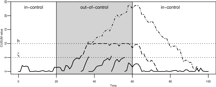
All charts are identical until they reach the threshold $\zeta$ for the first time. The non-restarting chart signals from time 33 to 66. So the out-of-control signal stops a few steps after the stream has returned to the in-control state. The restarting chart then signals at times 33, 37, 49, 56. The main downside of this is that it does not suggest a period where the stream is out-of-control and, importantly, there is no signal that the out-of-control period has ended. The boundary-free chart signals from 33 to 86. Clearly this lasts considerably longer than the out-of-control period. This is mainly due to the high values attained during the out-of-control period.

3 False Discovery Rate

3.1 Control of False Discovery Rate in Multiple Testing

We now consider monitoring multiple data streams using a non-restarting CUSUM chart with upper boundary (Section 2) for each stream. Instead of using a fixed threshold $\zeta$ to determine which streams are out of control, we suggest using an FDR control procedure. We first briefly review the procedure developed by Benjamini and Hochberg (1995).

Consider testing $N$ null hypotheses $H_{1}^{0},H_{2}^{0},\dots,H_{N}^{0}$ simultaneously. Denote the number of true null hypotheses by $m_{0}$. Let $V$ be the number of true null hypotheses declared significant and $R$ be the total of null hypotheses declared significant. Define $Q=V/R$ as the proportion of the rejected null hypotheses which are incorrectly rejected, with the convention $0/0=0$. The FDR is then defined as $E(Q)$.

Suppose we have $N$ independent tests with corresponding $p$-values $P_{1},P_{2},\dots,P_{N}$ for the hypotheses. The following algorithm proposed by Benjamini and Hochberg (1995) ensures the FDR is less than a pre-specified constant $q^{*}\in(0,1)$.

Algorithm 1 (Control of the FDR at $q^{*}\in(0,1)$)

1. Order the $p$-values as $P_{(1)}\leq P_{(2)}\leq\dots\leq P_{(N)}$, where $P_{(i)}$ corresponds to $H_{(i)}^{0}$.

2. Let $k$ be the largest $i$ for which $P_{(i)}\leq\frac{i}{N}q^{*}$.

3. Reject $H_{(i)}^{0}$ for $i=1,2,\dots,k.$

This procedure controls the FDR at $q^{*}$ i.e. $E(Q)\leq(m_{0}/N)q^{*}\leq q^{*}$. The procedure requires (Benjamini and Yekutieli, 2001, Th.5.1) that the $p$-values satisfy

$$\operatorname{pr}\left(P_{i}\leq\frac{k}{N}q^{*}\mid H_{i}^{0}\right)\leq\frac{k}{N}q^{*}\quad(k=0,\dots,N;i=1,2,\dots,N),$$ (3)

which is satisfied when $P_{i}$ is computed conditionally on $H_{i}^{0}$ being true (Lehmann and Romano, 2005, pg. 64, Lemma 3.3.1). The allocation of which null hypotheses are true can be random, and the FDR conditional on this allocation will still be controlled.

Based upon the above method, other FDR control procedures have been developed, e.g. the two-step FDR control procedure (Benjamini et al., 2006, Def. 6), the adaptive linear step-up procedure (Benjamini et al., 2006, Def. 3) and the adaptive step-down procedure (Gavrilov et al., 2009). These other procedures involve estimating $m_{0}$, by $\widehat{m}_{0}$ say, before applying the Benjamini and Hochberg (1995) procedure at level $q^{*}N/\widehat{m}_{0}$.

3.2 Algorithm

We wish to control the FDR at each time point using CUSUM charts for multiple streams. We first state the algorithm before precisely defining a false discovery in our setting.

Suppose we observe $N$ independent streams of observations $(Z_{i,t})_{t\in\mathbb{N}}$ $(i=1,\dots,N)$. Each $Z_{i,t}$ has distribution function $F_{i,t}$ with $F_{i,t}=F_{i,t}^{*}$ when $Z_{i,t}$ is in-control and $F_{i,t}\neq F_{i,t}^{*}$ when $Z_{i,t}$ is out-of-control. All $F_{i,t}^{*}$ are assumed to be known. For each stream $(Z_{i,t})_{t\in\mathbb{N}}$ we run a non-restarting CUSUM chart $S_{i,t}$ with upper boundary $h$ according to (2).

We propose the following algorithm to control the FDR at level $q^{*}\in(0,1)$ at each time $t$. Any FDR control procedure that controls the FDR at $q^{*}$ if (3) is guaranteed, can be used. These include the aforementioned two-step, adaptive linear step-up and adaptive step-down procedures.

The following algorithm is written for the homogeneous case where $F_{i,t}^{*}=F_{t}^{*}$ for all $i$.

Algorithm 2 (Control of the FDR at $q^{*}\in(0,1)$ at a fixed time $t$)

1. Let $(S_{\nu}^{*})_{\nu\in\mathbb{N}}$ be a chart with all observations in control, i.e. $F_{\nu}=F_{\nu}^{*}$ for all $\nu$. Compute the distribution of $S_{t}^{*}$ and let $P(s)=\operatorname{pr}(S_{t}^{*}\geq s)$.

2. For the observed streams ($i=1,\dots,N$) compute the $p$-values $P_{i,t}=P(S_{i,t})$.

3. Apply the chosen FDR procedure with level $q^{*}$ to the $p$-values $P_{1,t},\dots P_{N,t}$ . The rejected streams are signalled to be out-of-control.

It is straightforward to adapt this to the general case, where each stream can have a different in-control distribution or a different upper boundary, by computing the $p$-values separately for each stream.

If we use $\varphi$ in (2) to force the chart to take only finitely many values then Step 1 can be accomplished using Markov chains. Otherwise, $P(s)$ can be approximated through various methods such as a finite-state Markov chain approximation (Brook and Evans, 1972) or use of the steady state distribution of the CUSUM chart (Grigg and Spiegelhalter, 2008).

3.3 Null Hypothesis: In-Control Since Start

In this section we show that Algorithm 2 in Section 3.2 controls the FDR at a fixed time $t$ if a false discovery is defined as: a stream that signals out-of-control at time $t$, when it has in fact been in control since time $0$.

To phrase this in the language of hypothesis testing, the null hypotheses are

$$H_{i,t}^{0}=\left\{F_{i,\nu}=F_{i,\nu}^{*}\text{ }\text{ for all }0<\nu\leq t\right\}\quad(i=1,\dots,N).$$ (4)

A null hypothesis $H^{0}_{i,t}$ is declared significant when it is rejected by the FDR control procedure. Thus, at each time $t\in\mathbb{N}^{0}=\{0,1,2,\dots\}$,

$$V\!=\!\#\left\{i\!:\!F_{i,\nu}\!=\!F_{i,\nu}^{*}\text{ for all }0<\nu\leq t\text{, }H_{i,t}^{0}\text{ is significant}\right\}\text{ and }R\!=\!\#\left\{\text{significant hypotheses}\right\}.$$

The $p$-values are computed in agreement with the null hypotheses (4). Thus condition (3) holds and our algorithm (Algorithm 2 in Section 3.2) controls the FDR at $q^{*}$, i.e. $E(Q)=E\left(V/R\right)\leq q^{*}$.

3.4 Null Hypothesis: In-Control Since Visiting 0

The definition of a false discovery in the previous section implies that all discoveries made after a stream goes out of control for the first time are considered true discoveries. Thus a signal for a stream that has been out-of-control and then comes back in-control will never be considered a false discovery, no matter how long it has already been back in control.

In this section we show that Algorithm 2, without changing in the way the $p$-values are computed, also controls the FDR when a false discovery is defined as: a stream being signalled out-of-control at time $t$, when it has been in control since its chart was at $0$. The corresponding null hypotheses are

$$\widetilde{H}_{i,t}^{0}\!=\!\left\{\text{there exists }\tau\!\in\!\left\{0,\dots,t\right\}\text{:\ }S_{i,\tau}\!=\!0,F_{i,\nu}\!=\!F_{i,\nu}^{*}\text{ for all }\tau<\nu\leq t\right\}\quad(i=1,\dots,N).$$

Thus,

$$V\!\!=\!\#\!\left\{i:\widetilde{H}_{i,t}^{0}\text{ is significant and }\text{there exists }\tau\!:S_{i,\tau}\!=\!0,F_{i,\nu}\!=\!F_{i,\nu}^{*}\text{ for all }\tau<\nu\leq t\right\}\!.$$

The definitions of declared significant and $R$ remain the same as before. The $p$-values are computed as before. The following theorem shows that (3) is satisfied and thus the Benjamini and Hochberg (1995) FDR procedure still controls the FDR.

Theorem 1

For all $x\in[0,1]$ and for $t\in\mathbb{N}^{0}$,

$$\operatorname{pr}(P_{i,t}\leq x\mid\widetilde{H}_{i,t}^{0})\leq x\quad(i=1,\dots,N).$$

The proof can be found in Appendix 1. To summarize Theorem 1, the FDR with respect to both sets of hypotheses, $H_{i,t}^{0}$ and $\widetilde{H}_{i,t}^{0}$, is being controlled simultaneously.

4 Simulations

In this section we demonstrate the performance of our proposed method (Algorithm 2) under different definitions (Section 3.3 and Section 3.4) of a false discovery via simulations.

For each stream, we construct a CUSUM chart according to (2). In this simulation we let $F_{i,t}^{*}\sim N(-1/2,1)$ and $F_{i,t}\sim N(1/2,1)$ when out-of-control, for all $i,t\in\mathbb{N}$ and set the upper boundary $h=10$.

To compute the in-control CUSUM chart distribution, $S_{t}^{*}$, we use Brook and Evans (1972) method. If the chart is forced to take only finitely many values, by using the function $\varphi$ in (2), then the distribution can be computed exactly, as it is just the distribution of a finite-state Markov chain. We proceed by partitioning $[0,h]$ into the $M+1$ states by using

$$\varphi(x)=\begin{cases}0&x\in[0,w_{1})\\ (w_{j}+w_{j-1})/2&x\in[w_{j-1},w_{j})\quad(j=2,\dots,M)\\ h&x\in[w_{M},h]\end{cases}$$

where $w_{j}=\frac{h}{M}(j-\frac{1}{2})$ for $j=1,\dots,M$.

For each iteration we took $N=100$ streams over a period of 100 time points and partitioned $[0,h]$ into 100 states with $q^{*}=0.05$. A discrete time-homogeneous Markov chain is used to simulate the observations, for all charts, moving from in-control to out-of-control and vice versa. This Markov chain is defined by the transition probabilities $\operatorname{pr}(F_{i,t+1}=F_{i,t+1}^{*}\mid F_{i,t}\neq F_{i,t}^{*})=\alpha$ and $\operatorname{pr}(F_{i,t+1}\neq F_{i,t+1}^{*}\mid F_{i,t}=F_{i,t}^{*})=\beta$ for some known $0\leq\alpha,\beta\leq 1$ and for all $t\geq 0$ with all streams starting in control. In this simulation we let $\alpha=0.01$, $\beta=0.07$. This simulation was repeated 10,000 times, using the same seed. We consider the Benjamini and Hochberg (1995), the two-step and the adaptive linear step-up FDR control procedures.

(a)

(b)

(c)

(d)

Figure 2: (a) Example of a single CUSUM chart (solid) from the simulation with thresholds (dashed). The true out-of-control periods are given by the grey areas. (b) Median of $m_{0}$ (solid) with 95% (dashed) and 50% (dotted) quantile pointwise in time under $H_{i,t}^{0}$ (grey) and $\widetilde{H}_{i,t}^{0}$ (black). (c) Estimated FDR for the Benjamini and Hochberg (1995) (dotted), two-step (dashed) and adaptive linear step-up (solid) control procedures with $q^{*}=0.05$ using $H_{i,t}^{0}$. (d) same as (c) but using $\widetilde{H}_{i,t}^{0}$.

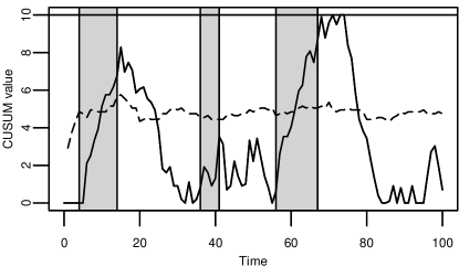
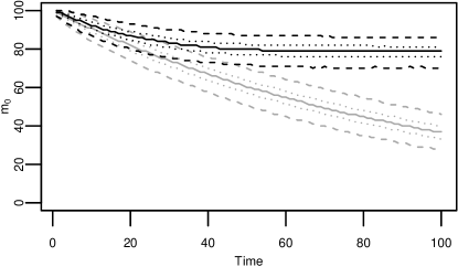
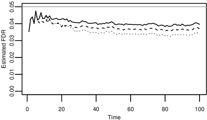
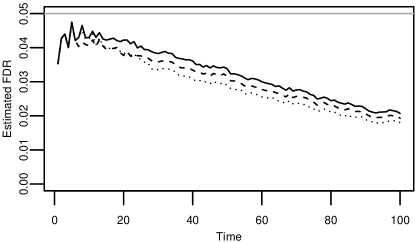
Figure 2a displays a CUSUM chart from a single iteration. The threshold given by the Benjamini and Hochberg (1995) FDR control procedure pointwise in time is also displayed. This threshold, based upon the remaining 99 charts in the same iteration, is the value which the presented CUSUM chart needs to exceed in order to signal out-of-control.

Figure 2c displays the FDR using these control procedures. All procedures control the FDR below $q^{*}=0.05$. However, the two-step and the adaptive linear step-up procedures control the FDR nearer to $q^{*}$ than the Benjamini and Hochberg (1995) FDR procedure. This is because other FDR control procedures estimate $m_{0}$ first, then apply the Benjamini and Hochberg (1995) procedure. For the same simulation, Figure 2d displays the FDR under the original hypotheses, $H_{i,t}^{0}$. We see the FDR for all the control procedures decreases over time, unlike in Figure 2c. This is explained by the lower number of true null hypotheses, $m_{0}$, at each time point under $H_{i,t}^{0}$ (Figure 2b).

5 Discussion

In the simulations in Section 4, we have used $\varphi$ to force the CUSUM chart to take only finitely many states. This ensures that the distribution of $S_{t}^{\ast}$ in Step 2 of Algorithm 2 can be computed exactly and thus the FDR is guaranteed to be controlled. Allowing the CUSUM chart to take continuous values, by using $\varphi(x)=x$, will no longer guarantee the control of the FDR as Step 2 of Algorithm 2 can only be done approximately. Further simulations, not reported here, showed that the false discovery rate was still controlled when using a Markov chain approximation with a reasonably large number of states. These simulations were similar to those in Section 4.

Ideally, we would like to define a false discovery as signalling out of control at time $t$ when in fact the observation is in control at time $t$, i.e. $F_{i,t}=F_{i,t}^{*}$. This is much stronger than our definitions of a false discovery - and thus the FDR will not be controlled under this stronger definition. It seems reasonable to assume that this FDR will depend on how quickly the observations switch between the in-control and the out-of-control state. Investigating this is a topic for further research.

Appendix 1

Proof of Theorem 1

Since each stream is independent we can drop the subscript $i$. We say a random variable $V$ is stochastically smaller than a random variable $Y$, denoted by $V\leq_{st}Y$, if $\operatorname{pr}(V\leq x)\geq\operatorname{pr}(Y\leq x)$ for all $x\in\mathbb{R}$.

We start the proof by showing, by induction on $t\in\mathbb{N}^{0}$, that

$$S_{t}\mid\widetilde{H}_{t}^{0}\leq_{st}S_{t}^{*}.$$ (5)

At time $t=0$, we have $S_{0}=S_{0}^{*}=0$ and $\operatorname{pr}(\widetilde{H}_{0}^{0})=1$, thus (5) holds.

At time $t\in\mathbb{N}$ consider the case $F_{t}\neq F_{t}^{*}$. Then $\widetilde{H}_{t}^{0}=\{S_{t}=0\}$ and $\operatorname{pr}(S_{t}\leq x\mid\widetilde{H}_{t}^{0})=1$ $\text{ for all }x\in\mathbb{R}$. Thus (5) holds for this case. For the case $F_{t}=F_{t}^{*}$, first assume (5) holds at time $(t-1)$. Hence, by the recursive definition of $S_{t}$ and $S_{t}^{*}$ in (2), and by the persistence of stochastic orders under convolution of independent random variables and under action of multiple increasing functions (Theorems 1.2.13 and 1.2.17 in Müller and Stoyan, 2002, pg. 6 and 7), we get $S_{t}\mid H_{t-1}^{0}=\varphi\left[\min\{\max(0,S_{t}+Z_{t}),h\}\right]\mid\widetilde{H}_{t-1}^{0}\leq_{st}S_{t}^{*}.$ Thus it suffices to show

$$S_{t}\mid\widetilde{H}_{t}^{0}\leq_{st}S_{t}\mid\widetilde{H}_{t-1}^{0}.$$ (6)

As $F_{t}=F_{t}^{*}$, we have $\widetilde{H}_{t}^{0}=\widetilde{H}_{t-1}^{0}\cup\{S_{t}=0\}$. Letting $G(x)=\operatorname{pr}(S_{t}\leq x\mid\widetilde{H}_{t}^{0})$, $J(x)=\operatorname{pr}(S_{t}\leq x\mid\widetilde{H}_{t-1}^{0})$ and $\alpha=\operatorname{pr}(\widetilde{H}_{t-1}^{0})/\operatorname{pr}(\widetilde{H}_{t}^{0})$, we have

$$G(x) =\operatorname{pr}(\{S_{t}\leq x,\widetilde{H}_{t-1}^{0}\}\cup\left\{S_{t}=0\right\})/\operatorname{pr}(\widetilde{H}_{t}^{0})$$

$$=\left\{\operatorname{pr}(S_{t}\leq x,\widetilde{H}_{t-1}^{0})+\operatorname{pr}(S_{t}=0)-\operatorname{pr}(S_{t}=0,\widetilde{H}_{t-1}^{0})\right\}\big{/}\operatorname{pr}(\widetilde{H}_{t}^{0})$$

$$=\left\{J(x)\operatorname{pr}(\widetilde{H}_{t-1}^{0})+\operatorname{pr}(S_{t}=0)-J(0)\operatorname{pr}(\widetilde{H}_{t-1}^{0})\right\}\big{/}\operatorname{pr}(\widetilde{H}_{t}^{0})$$

$$=\alpha J(x)-\alpha J(0)+\frac{\operatorname{pr}(S_{t}=0)}{\operatorname{pr}(\widetilde{H}_{t}^{0})}.$$ (7)

By setting $x=0$ in (7), we get $G(0)=\operatorname{pr}(S_{t}=0)/\operatorname{pr}(\widetilde{H}_{t}^{0})$, and so $G(x)-G(0)=\alpha\left(J(x)-J(0)\right)$.

The distribution of $S_{t}\mid\widetilde{H}_{t}^{0}$ is derived from the distribution of $S_{t}\mid\widetilde{H}_{t-1}^{0}$ by potentially adding mass at 0 before rescaling. Thus $0<\alpha\leq 1$ and $G(0)\geq J(0)$. Therefore, $G(x)-G(0)\geq J(x)-J(0).$ Hence, for all $x\in\mathbb{R}$, $G(x)\geq J(x)+\left\{G(0)-J(0)\right\}\geq J(x).$ Thus (6) holds. This finishes showing (5).

Since $P(\cdot)$, defined in Section 3.2, is a decreasing function, application of $P$ on (5) (an extension to Theorem 1.2.13 in Müller and Stoyan, 2002, pg. 6) yields

$$P_{t}\mid\widetilde{H}_{t}^{0}\geq_{st}P_{t}\mid H_{t}^{0}\quad(t\in\mathbb{N}^{0}).$$ (8)

By construction of $P_{t}$, we have

$$P_{t}\mid H_{t}^{0}\geq_{st}U,$$ (9)

where $U$ is uniformly distributed on $[0,1]$. Combining (8) and (9) gives

$$P_{t}\mid\widetilde{H}_{t}^{0}\geq_{st}P_{t}\mid H_{t}^{0}\geq_{st}U.$$

References

- Benjamini and Hochberg (1995) Y. Benjamini and Y. Hochberg. Controlling the false discovery rate: a practical and powerful approach to multiple testing. Journal of the Royal Statistical Society. Series B, 57(1):289–300, 1995.
- Benjamini and Kling (2007) Y. Benjamini and E. Y. Kling. The -valued chart - a unified approach to statistical process control chart presentation. (Available from www.businessken.com/papers/SPCpvalue.pdf), 2007.
- Benjamini and Kling (1999) Y. Benjamini and Y. Kling. A look at statistical process control through -values. Technical Report RP-SOR-99-08, Tel Aviv University, Israel, 1999.
- Benjamini and Yekutieli (2001) Y. Benjamini and D. Yekutieli. The control of the false discovery rate in multiple testing under dependency. The Annals of Statistics, 29(4):1165–1188, 2001.
- Benjamini et al. (2006) Y. Benjamini, A. M. Krieger, and D. Yekutieli. Adaptive linear step-up procedures that control the false discovery rate. Biometrika, 93(3):491–507, 2006.
- Biswas and Kalbfleisch (2008) P. Biswas and J. D. Kalbfleisch. A risk-adjusted CUSUM in continuous time based on the Cox model. Statistics in Medicine, 27(17):3382–3406, 2008.
- Bottle and Aylin (2008) A. Bottle and P. Aylin. Intelligent information: a national system for monitoring clinical performance. Health Services Research, 43(1 Pt 1):10–31, 2008.
- Brook and Evans (1972) D. Brook and D. A. Evans. An approach to the probability distribution of cusum run length. Biometrika, 59(3):539–549, 1972.
- Gavrilov et al. (2009) Y. Gavrilov, Y. Benjamini, and S. K. Sarkar. An adaptive step-down procedure with proven FDR control under independence. The Annals of Statistics, 37(2):619–629, 2009.
- Grigg and Spiegelhalter (2008) O. A. Grigg and D. J. Spiegelhalter. An empirical approximation to the null unbounded steady-state distribution of the cumulative sum statistic. Technometrics, 50(4):501–511, 2008.
- Hawkins and Olwell (1998) D. Hawkins and D. Olwell. Cumulative sum charts and charting for quality improvement. Statistics for engineering and physical science. Springer, 1998.
- Lehmann and Romano (2005) E. L. Lehmann and J. P. Romano. Testing statistical hypotheses. Springer Texts in Statistics. Springer, New York, third edition, 2005.
- Li and Tsung (2009) Y. Li and F. Tsung. False discovery rate-adjusted charting schemes for multistage process monitoring and fault identification. Technometrics, 51(2):186–205, 2009.
- Lucas and Crosier (1982) J. M. Lucas and R. B. Crosier. Fast initial response for cusum quality-control schemes: Give your cusum a head start. Technometrics, 24(3):199–205, 1982.
- Mei (2010) Y. Mei. Efficient scalable schemes for monitoring a large number of data streams. Biometrika, 97(2):419–433, 2010.
- Moustakides (1986) G. V. Moustakides. Optimal Stopping Times for Detecting Changes in Distributions. The Annals of Statistics, 14(4):1379–1387, 1986.
- Müller and Stoyan (2002) A. Müller and D. Stoyan. Comparison methods for stochastic models and risks. Wiley, 2002.
- Page (1954) E. S. Page. Continuous inspection schemes. Biometrika, 41(1-2):100–115, 1954.
- Spiegelhalter et al. (2012) D. Spiegelhalter, C. Sherlaw-Johnson, M. Bardsley, I. Blunt, C. Wood, and O. Grigg. Statistical methods for healthcare regulation: rating, screening and surveillance. Journal of the Royal Statistical Society, Series A, 175(1):1–47, 2012.