EP-GIG Priors and Applications in Bayesian Sparse Learning

Abstract

In this paper we propose a novel framework for the construction of sparsity-inducing priors. In particular, we define such priors as a mixture of exponential power distributions with a generalized inverse Gaussian density (EP-GIG). EP-GIG is a variant of generalized hyperbolic distributions, and the special cases include Gaussian scale mixtures and Laplace scale mixtures. Furthermore, Laplace scale mixtures can subserve a Bayesian framework for sparse learning with nonconvex penalization. The densities of EP-GIG can be explicitly expressed. Moreover, the corresponding posterior distribution also follows a generalized inverse Gaussian distribution. These properties lead us to EM algorithms for Bayesian sparse learning. We show that these algorithms bear an interesting resemblance to iteratively re-weighted $\ell_{2}$ or $\ell_{1}$ methods. In addition, we present two extensions for grouped variable selection and logistic regression.

Keywords: Sparsity priors, scale mixtures of exponential power distributions, generalized inverse Gaussian distributions, expectation-maximization algorithms, iteratively re-weighted minimization methods.

1 Introduction

In this paper we are concerned with sparse supervised learning problems over a training dataset ${{\mathcal{X}}}=\{({\bf x}_{i},y_{i})\}_{i=1}^{n}$. The point of departure for our work is the traditional formulation of supervised learning as a regularized optimization problem:

$$\min_{{\bf b}}\;\Big{\{}L({\bf b};{\mathcal{X}})+P_{\lambda}({\bf b})\Big{\}},$$

where ${\bf b}$ denotes the model parameter vector, $L(\cdot)$ the loss function penalizing data misfit, $P_{\lambda}(\cdot)$ the regularization term penalizing model complexity, and $\lambda>0$ the tuning parameter balancing the relative significance of the loss function and the penalty.

Variable selection is a fundamental problem in high-dimensional learning problems, and is closely tied to the notion that the data-generating mechanism can be described using a sparse representation. In supervised learning scenarios, the problem is to obtain sparse estimates for the regression vector ${\bf b}$. Given that it is NP-hard to use the $\ell_{0}$ penalty (i.e., the number of the nonzero elements of ${\bf b}$) (Weston et al., 2003), attention has focused on use of the $\ell_{1}$ penalty (Tibshirani, 1996). But in addition a number of studies have emphasized the advantages of nonconvex penalties—such as the bridge penalty and the log-penalty—for achieving sparsity (Fu, 1998, Fan and Li, 2001, Mazumder et al., 2011).

The regularized optimization problem can be cast into a maximum a posteriori (MAP) framework. This is done by taking a Bayesian decision-theoretic approach in which the loss function $L({\bf b};{\mathcal{X}})$ is based on the conditional likelihood of the output $y_{i}$ and the penalty $P_{\lambda}({\bf b})$ is associated with a prior distribution of ${\bf b}$. For example, the least-squares loss function is associated with Gaussian likelihood, while there exists duality between the $\ell_{1}$ penalty and the Laplace prior.

The MAP framework provides us with Bayesian underpinnings for the sparse estimation problem. This has led to Bayesian versions of the lasso, which are based on expressing the Laplace prior as a scale-mixture of a Gaussian distribution and an exponential density (Andrews and Mallows, 1974, West, 1987). Figueiredo (2003), and Kiiveri (2008) presented a Bayesian lasso based on the Expectation-Maximization (EM) algorithm. Caron and Doucet (2008) then considered an EM estimation with normal-gamma or normal-inverse-gaussian priors. In one latest work, Polson and Scott (2011b) proposed using generalized hyperbolic distributions, variance-mean mixtures of Gaussians with generalized inverse Gaussian densities. Moreover, Polson and Scott (2011b) devised EM algorithms via data augmentation methodology. However, these treatments is not fully Bayesian. Lee et al. (2010) referred to such a method based on MAP estimation as a quasi-Bayesian approach. Additionally, an empirical-Bayes sparse learning was developed by Tipping (2001).

Recently, Park and Casella (2008) and Hans (2009) proposed full Bayesian lasso models based on Gibbs sampling. Further work by Griffin and Brown (2010a) involved the use of a family of normal-gamma priors as a generalization of the Bayesian lasso. This prior has been also used by Archambeau and Bach (2009) to develop sparse probabilistic projections. In the work of Carvalho et al. (2010), the authors proposed horseshoe priors which are a mixture of normal distributions and a half-Cauchy density on the positive reals with scale parameter. Kyung et al. (2010) conducted performance analysis of Bayesian lassos in depth theoretically and empirically.

There has also been work on nonconvex penalties within a Bayesian framework. Zou and Li (2008) derived their local linear approximation (LLA) algorithm by combining the EM algorithm with an inverse Laplace transformation. In particular, they showed that the bridge penalty can be obtained by mixing the Laplace distribution with a stable distribution. Other authors have shown that the prior induced from the log-penalty has an interpretation as a scale mixture of Laplace distributions with an inverse gamma density (Cevher, 2009, Garrigues and Olshausen, 2010, Lee et al., 2010, Armagan et al., 2011). Additionaly, Griffin and Brown (2010b) devised a family of normal-exponential-gamma priors for a Bayesian adaptive lasso (Zou, 2006). Polson and Scott (2010, 2011a) provided a unifying framework for the construction of sparsity priors using Lévy processes.

In this paper we develop a novel framework for constructing sparsity-inducing priors. Generalized inverse Gaussian (GIG) distributions (Jørgensen, 1982) are conjugate with respect to an exponential power (EP) distribution (Box and Tiao, 1992)—an extension of Gaussian and Laplace distributions. Accordingly, we propose a family of distributions that we refer to as EP-GIG. In particular, we define EP-GIG as a scale mixture of EP distributions with a GIG density, and derive their explicit densities. EP-GIG can be regarded as a variant of generalized hyperbolic distributions, and include Gaussian scale mixtures and Laplacian scale mixtures as special cases. The Gaussian scale mixture is a class of generalized hyperbolic distributions (Polson and Scott, 2011b) and its special cases include normal-gamma distributions (Griffin and Brown, 2010a) as well as the Laplacian distribution. The generalized double Pareto distribution in (Cevher, 2009, Armagan et al., 2011, Lee et al., 2010) and the bridge distribution inducing the $\ell_{1/2}$ bridge penalty (Zou and Li, 2008) are special cases of Laplacian scale mixtures. In Appendix B, we devise a set of now EP-GIG priors.

Since GIG priors are conjugate with respect to EP distributions, it is feasible to apply EP-GIG to Bayesian sparse learning. Although it has been illustrated that fully Bayesian sparse learning methods based on Markov chain Monte Carlo sampling work well, our main attention is paid to a quasi-Bayesian approach. The important purpose is to explore the equivalent relationship between the MAP estimator and the classical regularized estimator in depth. In particular, using the property of EP-GIG as a scale-mixture of exponential power distributions, we devise EM algorithms for finding a sparse MAP estimate of ${\bf b}$.

When we set the exponential power distribution to be the Gaussian distribution, the resulting EM algorithm is closely related to the iteratively re-weighted $\ell_{2}$ minimization methods in (Daubechies et al., 2010, Chartrand and Yin, 2008, Wipf and Nagarajan, 2010). When we employ the Laplace distribution as a special exponential power distribution, we obtain an EM algorithm which is identical to the iteratively re-weighted $\ell_{1}$ minimization method in (Candès et al., 2008). Interestingly, using a bridge distribution of order $q$ ($0<q<1$) results in an EM algorithm, which in turn corresponds to an iteratively re-weighted $\ell_{q}$ method.

We also develop hierarchical Bayesian approaches for grouped variable selection (Yuan and Lin, 2007) and penalized logistic regression by using EP-GIG priors. We apply our proposed EP-GIG priors in Appendix B to conduct experimental analysis. The experimental results validate that those proposed EP-GIG priors which induce nonconvex penalties are potentially feasible and effective in sparsity modeling. Finally, we would like to highlight that our work offers several important theorems as follows.

1. Theorems 5, 6 and 7 recover the relationship of EP-GIG with the corresponding EP at the limiting case. These theorems extend the fact that the $t$-distribution degenerates to Gaussian distribution as the degree of freedom approaches infinity.

2. Theorem 8 proves that an exponential power distribution of order $q/2$ ($q>0$) can be always represented a scale mixture of exponential power distributions of order $q$ with a gamma mixing density.

3. The first part of Theorem 9 shows that GIG is conjugate with respect to EP, while the second part then offers a theoretical evidence of relating EM algorithms with iteratively re-weighted minimization methods under our framework.

4. Theorem 10 shows that the negative log EP-GIG can induce a class of sparsity penalties. Especially, it shows a class of nonconvex penalties. Finally, Theorem 11 establishes the oracle properties of the sparse estimator based on Laplace scale mixture priors.

The paper is organized as follows. A brief reviewe about exponential power distributions and generalized inverse Gaussian distributions is given in Section 2. Section 3 presents EP-GIG distributions and their some properties, Section 4 develops our EM algorithm for Bayesian sparse learning, and Section 5 discusses the equivalent relationship between the EM and iteratively re-weighted minimization methods. In Section 6 we conduct our experimental evaluationsd. Finally, we conclude our work in Section 7, defer all proofs to Appendix A, and provide several new sparsity priors in Appendix B.

2 Preliminaries

Before presenting EP-GIG priors for sparse modeling of regression vector ${\bf b}$, we give some notions such as the exponential power (EP) and generalized inverse Gaussian (GIG) distributions.

2.1 Exponential Power Distributions

For a univariate random variable $b\in{\mathbb{R}}$, it is said to follow an EP distribution if the density is specified by

$$p(b)=\frac{\eta^{-1/q}}{2^{\frac{q+1}{q}}\Gamma(\frac{q{+}1}{q})}\exp(-\frac{1}{2\eta}|b-u|^{q})=\frac{q}{2}\frac{(2\eta)^{-\frac{1}{q}}}{\Gamma(\frac{1}{q})}\exp(-\frac{1}{2\eta}|b-u|^{q}),$$

with $\eta>0$. In the literature (Box and Tiao, 1992), it is typically assumed that $q\geq 1$. However, we find that it is able to relax this assumption into $q>0$ without any obstacle. Thus, we assume $q>0$ for our purpose. Moreover, we will set $u=0$.

The distribution is denoted by ${\mathsf{EP}}(b|u,\eta,q)$. There are two classical special cases: the Gaussian distribution arises when $q=2$ (denoted $N(b|u,\eta)$) and the Laplace distribution arises when $q=1$ (denoted $L(b|u,\eta)$). As for the case that $q<1$, the corresponding density induces a bridge penalty for $b$. We thus refer to it as the bridge distribution.

2.2 Generalized Inverse Gaussian Distributions

We first let $G(\eta|\tau,\theta)$ denote the gamma distribution whose density is

$$p(\eta)=\frac{\theta^{\tau}}{\Gamma(\tau)}\eta^{\tau-1}\exp(-\theta\eta),\quad\tau,\theta>0,$$

and $\mathsf{IG}(\eta|\tau,\theta)$ denote the inverse gamma distribution whose density is

$$p(\eta)=\frac{\theta^{\tau}}{\Gamma(\tau)}\eta^{-(1+\tau)}\exp(-\theta\eta^{-1}),\quad\tau,\theta>0.$$

An interesting property of the gamma and inverse gamma distributions is given as follows.

Proposition 1

Let $\lambda>0$. Then

1. $\lim_{\tau\rightarrow\infty}G(\eta|\tau,\tau\lambda)=\delta(\eta|1/\lambda)$.

2. $\lim_{\tau\rightarrow\infty}\mathsf{IG}(\eta|\tau,\tau/\lambda)=\delta(\eta|1/\lambda)$.

Here $\delta(\eta|a)$ is the Dirac delta function; namely,

$$\delta(\eta|a)=\left\{\begin{array}[]{ll}\infty&\mbox{if }\eta=a,\\ 0&\mbox{otherwise}.\end{array}\right.$$

We now consider the GIG distribution. The density of GIG is defined as

$$p(\eta)=\frac{(\alpha/\beta)^{\gamma/2}}{2K_{\gamma}(\sqrt{\alpha\beta})}\eta^{\gamma-1}\exp(-(\alpha\eta+\beta\eta^{-1})/2),\;\eta>0,$$ (1)

where $K_{\gamma}(\cdot)$ represents the modified Bessel function of the second kind with the index $\gamma$. We denote this distribution by ${\mathsf{GIG}}(\eta|\gamma,\beta,\alpha)$. It is well known that its special cases include the gamma distribution $G(\eta|\gamma,\alpha/2)$ when $\beta=0$ and $\gamma>0$, the inverse gamma distribution $\mathsf{IG}(\eta|-\gamma,\beta/2)$ when $\alpha=0$ and $\gamma<0$, the inverse Gaussian distribution when $\gamma=-1/2$, and the hyperbolic distribution when $\gamma=0$. Please refer to Jørgensen (1982) for the details.

Note in particular that the pdf of the inverse Gaussian ${\mathsf{GIG}}(\eta|{-}1/2,\beta,\alpha)$ is

$$p(\eta)=\Big{(}\frac{\beta}{2\pi}\Big{)}^{1/2}\exp(\sqrt{\alpha\beta})\eta^{-\frac{3}{2}}\exp(-(\alpha\eta+\beta\eta^{-1})/2),\;\beta>0,$$ (2)

and the pdf of ${\mathsf{GIG}}(\eta|1/2,\beta,\alpha)$ is

$$p(\eta)=\Big{(}\frac{\alpha}{2\pi}\Big{)}^{1/2}\exp(\sqrt{\alpha\beta})\eta^{-\frac{1}{2}}\exp(-(\alpha\eta+\beta\eta^{-1})/2),\;\alpha>0.$$ (3)

Note moreover that ${\mathsf{GIG}}(\eta|{-}1/2,\beta,0)$ and ${\mathsf{GIG}}(\eta|1/2,0,\alpha)$ degenerate to $\mathsf{IG}(\eta|1/2,\beta/2)$ and $G(\eta|1/2,\alpha/2)$, respectively.

As an extension of Proposition 1, we have the limiting property of GIG as follows.

Proposition 2

Let $\alpha>0$ and $\beta>0$. Then

1. $\lim_{\gamma\rightarrow+\infty}\mathsf{GIG}(\eta|\gamma,\beta,\gamma\alpha)=\delta(\eta|2/\alpha)$.

2. $\lim_{\gamma\rightarrow-\infty}\mathsf{GIG}(\eta|\gamma,-\gamma\beta,\alpha)=\delta(\eta|\beta/2)$.

We now present an alternative expression for the GIG density that is also interesting. Let $\psi=\sqrt{\alpha\beta}$ and $\phi=\sqrt{\alpha/\beta}$. We can rewrite the density of $\mathsf{GIG}(\eta|\gamma,\beta,\alpha)$ as

$$p(\eta)=\frac{\phi^{\gamma}}{2K_{\gamma}(\psi)}\eta^{\gamma-1}\exp(-\psi(\phi\eta+(\phi\eta)^{-1})/2),\;\eta>0.$$ (4)

Proposition 3

Let $p(\eta)$ be defined by (4) where $\phi$ is a positive constant and $\gamma$ is a any constant. Then

$$\lim_{\psi+\infty}p(\eta)=\delta(\eta|\phi).$$

Finally, let us consider that the case $\gamma=0$. Furthermore, letting $\psi\rightarrow 0$, we can see that $p(\eta)\propto 1/\eta$, an improper prior. Note that this improper prior can regarded as the Jeffreys prior because the Fisher information of $\mathsf{EP}(b|0,\eta)$ with respect to $\eta$ is $\eta^{-2}/q$.

3 EP-GIG Distributions

We now develop a family of distributions by mixing the exponential power ${\mathsf{EP}}(b|0,\eta,q)$ with the generalized inverse Gaussian ${\mathsf{GIG}}(\eta|\gamma,\beta,\alpha)$. The marginal density of $b$ is currently defined by

$$p(b)=\int_{0}^{+\infty}{{\mathsf{EP}}(b|0,\eta,q){\mathsf{GIG}}(\eta|\gamma,\beta,\alpha)d\eta}.$$

We refer to this distribution as the EP-GIG and denote it by ${\mathsf{EGIG}}(b|\alpha,\beta,{\gamma},q)$.

Theorem 4

Let $b\sim{\mathsf{EGIG}}(b|\alpha,\beta,{\gamma},q)$. Then its density is

$$p(b)=\frac{K_{\frac{\gamma q{-}1}{q}}(\sqrt{\alpha(\beta{+}|b|^{q})})}{2^{\frac{q+1}{q}}\Gamma(\frac{q{+}1}{q})K_{\gamma}(\sqrt{\alpha\beta})}\frac{\alpha^{1/(2q)}}{\beta^{{\gamma}/2}}[\beta{+}|b|^{q}]^{(\gamma q-1)/(2q)}.$$ (5)

The following theorem establishes an important relationship of an EP-GIG with the corresponding EP distribution. It is an extension of the relationship of a $t$-distribution with the Gaussian distribution. That is,

Theorem 5

Consider EP-GIG distributions. Then

1. $\lim_{\gamma\rightarrow+\infty}\mathsf{EGIG}(b|\gamma\alpha,\beta,\gamma,q)=\mathsf{EP}(b|0,2/\alpha,q)$;

2. $\lim_{\gamma\rightarrow-\infty}\mathsf{EGIG}(b|\alpha,-\gamma\beta,\gamma,q)=\mathsf{EP}(b|0,\beta/2,q)$.

3. $\lim_{\psi\rightarrow+\infty}\mathsf{EGIG}(b|\alpha,\beta,\gamma,q)=\mathsf{EP}(b|0,\phi,q)$ where $\psi=\sqrt{\alpha\beta}$ and $\phi=\sqrt{\alpha/\beta}\in(0,\infty)$.

EP-GIG can be regarded as a variant of generalized hyperbolic distributions (Jørgensen, 1982), because when $q=2$ EP-GIG is generalized hyperbolic distributions—a class of Gaussian scale mixtures. However, EP-GIG becomes a class of Laplace scale mixtures when $q=1$.

In Appendix B we present several new concrete EP-GIG distributions, obtained from particular settings of ${\gamma}$ and $q$. We now consider the two special cases that mixing density is either a gamma distribution or an inverse gamma distribution. Accordingly, we have two special EP-GIG: exponential power-gamma distributions and exponential power-inverse gamma distributions.

3.1 Generalized $t$ Distributions

We first consider an important family of EP-GIG distributions, which are scale mixtures of exponential power $\mathsf{EP}(b|u,\eta,q)$ with inverse gamma $\mathsf{IG}(\eta|\tau/2,\tau/(2\lambda))$. Following the terminology of Lee et al. (2010), we refer them as generalized $t$ distributions and denote them by $\mathsf{GT}(b|u,\tau/\lambda,\tau/2,q)$. Specifically, the density of the generalized $t$ is

$$p(b)=\int{\mathsf{EP}(b|u,\eta,q)\mathsf{IG}(\eta|\tau/2,\tau/(2\lambda))d\eta}=\frac{q}{2}\frac{\Gamma(\frac{\tau}{2}{+}\frac{1}{q})}{\Gamma(\frac{\tau}{2})\Gamma(\frac{1}{q})}\Big{(}\frac{\lambda}{\tau}\Big{)}^{\frac{1}{q}}\Big{(}1+\frac{\lambda}{\tau}|b-u|^{q}\Big{)}^{-(\frac{\tau}{2}+\frac{1}{q})}$$ (6)

where $\tau>0$, $\lambda>0$ and $q>0$. Clearly, when $q=2$ the generalized $t$ distribution becomes to a $t$-distribution. Moreover, when $\tau=1$, it is the Cauchy distribution.

On the other hand, when $q=1$, Cevher (2009) and Armagan et al. (2011) called the resulting generalized $t$ generalized double Pareto distributions (GDP). The density of GDP is specified as

$$p(b)=\int_{0}^{\infty}{L(b|0,\eta)\mathsf{IG}(\eta|\tau/2,\tau/(2\lambda))}d\eta=\frac{\lambda}{4}\Big{(}1+\frac{\lambda|b|}{\tau}\Big{)}^{-(\tau/2+1)},\quad\lambda>0,\tau>0.$$ (7)

Furthermore, we let $\tau=1$; namely, $\eta\sim\mathsf{IG}(\eta|1/2,1/(2\lambda))$. As a result, we obtain

$$p(b)=\frac{\lambda}{4}(1+\lambda|b|)^{-3/2},$$

It is well known that the limit of the $t$-distribution at $\tau\rightarrow\infty$ is the normal distribution. We find that we are able to extend this property to the generalized $t$ distribution. In particular, we have the following theorem, which is in fact a corollary of the first part of Theorem 5.

Theorem 6

Let the generalized $t$ distribution be defined in (6). Then, for $\lambda>0$ and $q>0$,

$$\lim_{\tau\rightarrow\infty}\mathsf{GT}(b|u,\tau/\lambda,\tau/2,q)=\mathsf{EP}(b|u,1/\lambda,q).$$

Thus, as a special case of Theorem 6 in $q=1$, we have

$$\lim_{\tau\rightarrow\infty}\mathsf{GT}(b|u,\tau/\lambda,\tau/2,1)=L(b|u,1/\lambda).$$

3.2 Exponential Power-Gamma Distributions

In particular, the density of the exponential power-gamma distribution is defined by

$$p(b|\gamma,\alpha)=\int_{0}^{\infty}{\mathsf{EP}(b|0,\eta,q)G(\eta|\gamma,\alpha/2)}d\eta=\frac{\alpha^{\frac{q\gamma+1}{2q}}|b|^{\frac{q\gamma-1}{2}}}{2^{\frac{q\gamma{+}1}{q}}\Gamma(\frac{q{+}1}{q})\Gamma(\gamma)}K_{\gamma-\frac{1}{q}}(\sqrt{\alpha|b|^{q}}),\gamma,\alpha>0.$$

We denote the distribution by $\mathsf{EG}(b|\alpha,\gamma,q)$. As a result, the density of the normal-gamma distribution (Griffin and Brown, 2010a) is

$$p(b|\gamma,\alpha)=\int_{0}^{\infty}{N(b|0,\eta)G(\eta|\gamma,\alpha/2)}d\eta=\frac{\alpha^{\frac{2\gamma+1}{4}}|b|^{\gamma-\frac{1}{2}}}{2^{\gamma-\frac{1}{2}}\sqrt{\pi}\Gamma(\gamma)}K_{\gamma-\frac{1}{2}}(\sqrt{\alpha}|b|),\quad\gamma,\alpha>0.$$ (8)

As the application of the second part of Theorem 5 in this case, we can obtain the following theorem.

Theorem 7

Let $\mathsf{EG}(b|\lambda\gamma,\gamma/2,q)=\int_{0}^{\infty}{\mathsf{EP}(b|0,\eta,q)G(\eta|\gamma/2,\lambda\gamma/2)}d\eta$ with $\lambda>0$. Then

$$\lim_{\gamma\rightarrow\infty}\mathsf{EG}(b|\lambda\gamma,\gamma/2,q)=\mathsf{EP}(b|0,1/\lambda,q).$$

It is easily seen that when we let $\gamma=1$, the normal-gamma distribution degenerates to the Laplace distribution $L(b|0,\alpha^{-1/2}/2)$. In addition, when $q=1$ and $\gamma=3/2$ which implies that $[b|\eta]\sim L(b|0,\eta)$ and $\eta\sim G(\eta|3/2,\alpha/2)$, we have

$$p(b|\alpha)=\frac{\alpha}{4}\exp(-\sqrt{\alpha|b|})=\int_{0}^{+\infty}{L(b|0,\eta)G(\eta|3/2,\alpha/2)d\eta}.$$ (9)

Obviously, the current exponential power-gamma is identical to exponential power distribution $\mathsf{EP}(b|0,\alpha^{-1/2}/2,1/2)$, a bridge distribution with $q=1/2$. Interestingly, we can extend this relationship between the Gaussian and Laplace as we as between the Laplace and $1/2$-bridge to the general case. That is,

Theorem 8

Let $\gamma=\frac{1}{2}+\frac{1}{q}$. Then,

$$\mathsf{EP}(b|0,\alpha^{-1/2}/2,q/2)=\frac{q\alpha^{{1}/{q}}}{4\Gamma({2}/{q})}\exp(-\sqrt{\alpha|b|^{q}})=\int_{0}^{+\infty}{\mathsf{EP}(b|0,\eta,q)G(\eta|\gamma,\alpha/2)d\eta}.$$

This theorem implies that a $q/2-$bridge distribution can be represented as a scale mixture of $q-$bridge distributions. A class of important settings are $q=2^{1{-}m}$ and $\gamma=\frac{1}{2}+\frac{1}{q}=\frac{1+2^{m}}{2}$ where $m$ is any nonnegative integer.

3.3 Conditional Priors, Marginal Priors and Posteriors

We now study the posterior distribution of $\eta$ conditioning on $b$. It is immediate that the posterior distribution follows ${\mathsf{GIG}}(\eta|(\gamma q{-}1)/q,(\beta+|b|^{q}),\alpha)$. This implies that GIG distributions are conjugate with respect to the EP distribution. We note that in the cases $\gamma=1/2$ and $q=1$ as well as $\gamma=0$ and $q=2$, the posterior distribution is ${\mathsf{GIG}}(\eta|{-}1/2,(\beta+|b|^{q}),\alpha)$. In the cases $\gamma=3/2$ and $q=1$ as well as $\gamma=1$ and $q=2$, the posterior distribution is ${\mathsf{GIG}}(\eta|1/2,(\beta+|b|^{q}),\alpha)$. When $\gamma=-1/2$ and $q=1$ or $\gamma=-1$ and $q=2$, the posterior distribution is ${\mathsf{GIG}}(\eta|{-}3/2,(\beta+|b|^{q}),\alpha)$.

Additionally, we have the following theorem.

Theorem 9

Suppose that $b|\eta\sim\mathsf{EP}(b|0,\eta,q)$ and $\eta\sim\mathsf{GIG}(\eta|\gamma,\beta,\alpha)$. Then

1. $b\sim\mathsf{EGIG}(b|\alpha,\beta,\gamma,q)$ and $\eta|b\sim\mathsf{GIG}(\eta|(\gamma q{-}1)/q,(\beta+|b|^{q}),\alpha)$.

2. $\frac{\partial-\log p(b)}{\partial|b|^{q}}=\frac{1}{2}E(\eta^{-1}|b)=\frac{1}{2}\int{\eta^{-1}p(\eta|b)d\eta}$.

When as a penalty $-\log p(b)$ is applied to supervised sparse learning, iterative re-weighted $\ell_{1}$ or $\ell_{2}$ local methods are suggested for solving the resulting optimization problem. We will see that Theorem 9 shows the equivalent relationship between an iterative re-weighted method and an EM algorithm, which is presented in Section 4.

3.4 Duality between Priors and Penalties

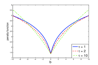
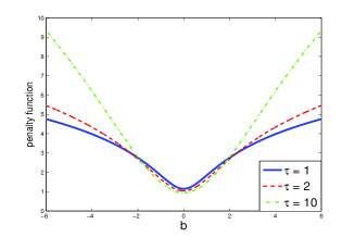
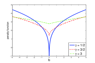
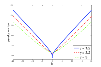
Since there is duality between a prior and a penalty, we are able to construct a penalty from $p(b)$; in particular, $-\log p(b)$ corresponds to a penalty. For example, let $p(b)$ be defined as in (13) or (14) (see Appendix B). It is then easily checked that $-\log p(b)$ is concave in $|b|$. Moreover, if $p(b)$ is given in (9), then $-\log p(b)$ induces the $\ell_{1/2}$ penalty $|b|^{1/2}$. In fact, we have the following theorem.

Theorem 10

Let $p(b)$ be the EP-GIG density given in (5). If $-\log p(b)$ is regarded as a function of $|b^{q}|$, then $-\frac{d\log(p(b))}{d|b|^{q}}$ is completely monotone on $(0,\infty)$. Furthermore, when $0<q\leq 1$, ${-}\log(p(b))$ is concave in $|b|$ on $(0,\infty)$; namely, ${-}\log(p(b))$ defines a class of nonconvex penalties for $b$.

Here a function $\phi(z)$ on $(0,\infty)$ is said to be completely monotone (Feller, 1971) if it possesses derivatives $\phi^{(n)}$ of all orders and

$$(-1)^{n}\phi^{(n)}(z)\geq 0,\;z>0.$$

Theorem 10 implies that the first-order and second-order derivatives of $-\log(p(b))$ with respect to $|b|^{q}$ are nonnegative and nonpositive, respectively. Thus, ${-}\log(p(b))$ is concave and nondecreasing in $|b|^{q}$ on $(0,\infty)$. Additionally, $|b|^{q}$ for $0<q\leq 1$ is concave in $|b|$ on $(0,\infty)$. Consequently, when $0<q\leq 1$, ${-}\log(p(b))$ is concave in $|b|$ on $(0,\infty)$. In other words, ${-}\log(p(b))$ with $0<q\leq 1$ induces a nonconvex penalty for $b$.

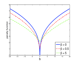
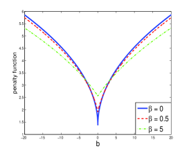
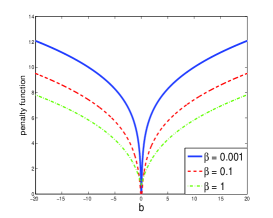
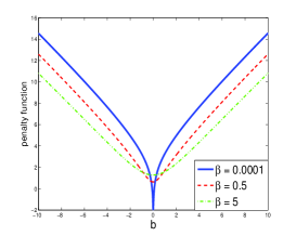
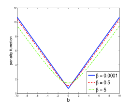
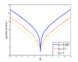
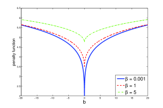
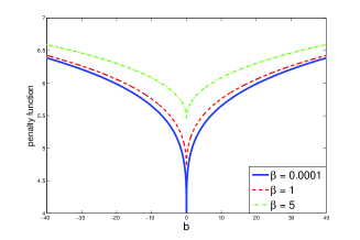
Figure 1 graphically depicts several penalties, which are obtained from the special priors in Appendix B. It is readily seen that the fist three penalty functions are concave in $|b|$ on $(0,\infty)$. In Figure 2, we also illustrate the penalties induced from the $1/2$-bridge scale mixture priors (see Examples 7 and 8 in in Appendix B), generalized $t$ priors and EP-G priors. Again, we see that the two penalties induced from the $1/2$-bridge mixture priors are concave in $|b|$ on $(0,\infty)$. This agrees with Theorem 10.

(a) $\gamma=\frac{1}{2}$, $q=1$

(b) $\gamma=\frac{3}{2}$, $q=1$

(c) $\gamma=-\frac{1}{2}$, $q=1$

(d) $\gamma=0$, $q=2$

(e) $\gamma=1$, $q=2$

(f) $\gamma=-1$, $q=2$

Figure 1: Penalty functions induced from exponential power-generalized inverse gamma (EP-GIG) priors in which $\alpha=1$.

(a) EP-GIG$(\gamma=\frac{3}{2}$, $q=\frac{1}{2},\alpha=1)$

(b) EP-GIG$(\gamma=\frac{5}{2}$, $q=\frac{1}{2},\alpha=1)$

(c) GT (or GDP) ($q=1$ and $\lambda=1$)

(d) GT ($q=2$ and $\lambda=1$)

(e) EG ($q=1$ and $\lambda=1$)

(f) EG ($q=2$ and $\lambda=1$)

Figure 2: Penalty functions induced from $1/2$-bridge scale mixture priors, exponential power-inverse gamma (or generalized $t$, GT) priors and exponential power-gamma (EG) priors.

4 Bayesian Sparse Learning Methods

In this section we apply EP-GIG priors to empirical Bayesian sparse learning. Suppose we are given a set of training data $\{({\bf x}_{i},y_{i}):i=1,\ldots,n\}$, where the ${\bf x}_{i}\in{\mathbb{R}}^{p}$ are the input vectors and the $y_{i}$ are the corresponding outputs. Moreover, we assume that $\sum_{i=1}^{n}{\bf x}_{i}={\bf 0}$ and $\sum_{i=1}^{n}y_{i}=0$. We now consider the following linear regression model:

$${\bf y}={\bf X}{\bf b}+\mbox{\boldmath$\varepsilon$\unboldmath},$$

where ${\bf y}=(y_{1},\ldots,y_{n})^{T}$ is the $n{\times}1$ output vector, ${\bf X}=[{\bf x}_{1},\ldots,{\bf x}_{n}]^{T}$ is the $n{\times}p$ input matrix, and $\varepsilon$ is a Gaussian error vector $N(\mbox{\boldmath$\varepsilon$\unboldmath}|{\bf 0},\sigma{\bf I}_{n})$. We aim to estimate the vector of regression coefficients ${\bf b}=(b_{1},\ldots,b_{p})^{T}$ under the MAP framework.

4.1 Bayesian Sparse Regression

We place an EP-GIG prior on each of the elements of ${\bf b}$. That is,

$$p({\bf b}|\sigma)=\prod_{j=1}^{p}\mathsf{EGIG}(b_{j}|\sigma^{-1}\alpha,\sigma\beta,\gamma,q).$$

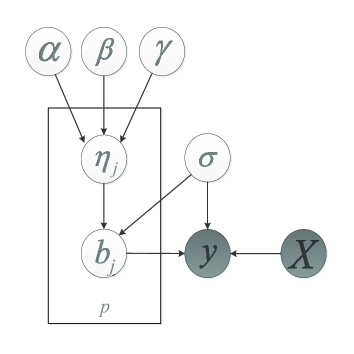
Using the property the the EP-GIG distribution is a scale mixture of exponential power distributions, we devise an EM algorithm for the MAP estimate of ${\bf b}$. For this purpose, we define a hierarchical model:

$$[{\bf y}|{\bf b},\sigma] \sim N({\bf y}|{\bf X}{\bf b},\sigma{\bf I}_{n}),$$

$$[b_{j}|\eta_{j},\sigma] \stackrel{{\scriptstyle ind}}{{\sim}}\mathsf{EP}(b_{j}|0,\sigma\eta_{j},q),$$

$$[\eta_{j}|\gamma,\beta,\alpha] \stackrel{{\scriptstyle iid}}{{\sim}}\mathsf{GIG}(\eta_{j}|\gamma,\beta,\alpha),$$

$$p(\sigma) =``Constant".$$

According to Section 3.3, we have

$$[\eta_{j}|b_{j},\sigma,\alpha,\beta,\gamma]\sim\mathsf{GIG}\big{(}\eta_{j}\big{|}(\gamma q{-}1)/q,\;\beta{+}\sigma^{-1}|b_{j}|^{q},\;\alpha\big{)}.$$

Given the $t$th estimates $({\bf b}^{(t)},\sigma^{(t)})$ of $({\bf b},\sigma)$, the E-step of EM calculates

$$Q({\bf b},\sigma|{\bf b}^{(t)},\sigma^{(t)}) \triangleq\log p({\bf y}|{\bf b},\sigma)+\sum_{j=1}^{p}\int{\log p[b_{j}|\eta_{j},\sigma]p(\eta_{j}|b_{j}^{(t)},\sigma^{(t)},\alpha,\beta,\gamma)}d\eta_{j}$$

$$\propto-\frac{n}{2}\log\sigma{-}\frac{1}{2\sigma}({\bf y}{-}{\bf X}{\bf b})^{T}({\bf y}{-}{\bf X}{\bf b})-\frac{p}{q}\log\sigma$$

$$\quad-\frac{1}{2\sigma}\sum_{j=1}^{p}|b_{j}|^{q}\int\eta_{j}^{-1}p(\eta_{j}|b_{j}^{(t)},\sigma^{(t)},\alpha,\beta,\gamma)d\eta_{j}.$$

Here we omit some terms that are independent of parameters $\sigma$ and ${\bf b}$. In fact, we only need calculating $E(\eta_{j}^{-1}|b_{j}^{(t)},\sigma^{(t)})$ in the E-step. It follows from Proposition 17 (see Appendix A) that

$$w_{j}^{(t{+}1)}\triangleq E(\eta_{j}^{-1}|b_{j}^{(t)},\sigma^{(t)})=\frac{\alpha^{1/2}}{\big{[}\beta{+}|b^{(t)}_{j}|^{q}/\sigma^{(t)}\big{]}^{1/2}}\frac{K_{(\gamma q{-}q{-}1)/q}\big{(}\sqrt{\alpha[\beta{+}|b^{(t)}_{j}|^{q}/\sigma^{(t)}]}\big{)}}{K_{(\gamma q{-}1)/q}\big{(}\sqrt{\alpha[\beta{+}|b^{(t)}_{j}|^{q}/\sigma^{(t)}]}\big{)}}.$$ (10)

There do not exist analytic computational formulae for arbitrary modified Bessel functions $K_{\nu}$. In this case, we can resort to a numerical approximation to the Bessel function. Fortunately, once $\gamma$ and $q$ take the special values in Appendix B, we have closed-form expressions for the corresponding Bessel functions and thus for the $w_{j}$. In particular, we have from Proposition 18 (see Appendix A) that

$$w_{j}^{(t{+}1)}=\left\{\begin{array}[]{ll}\Big{[}\frac{\sigma^{(t)}\alpha}{\sigma^{(t)}\beta+|b_{j}^{(t)}|^{q}}\Big{]}^{1/2}&(\gamma q{-}1)/q=1/2,\\ \frac{\sigma^{(t)}+[\sigma^{(t)}\alpha(\sigma^{(t)}\beta+|b_{j}^{(t)}|^{q})]^{1/2}}{\sigma^{(t)}\beta+|b_{j}^{(t)}|^{q}}&(\gamma q{-}1)/q=-1/2,\\ \frac{3\sigma^{(t)}}{\sigma^{(t)}\beta+|b_{j}^{(t)}|^{q}}+\frac{\sigma^{(t)}\alpha}{\sigma^{(t)}+[\sigma^{(t)}\alpha(\sigma^{(t)}\beta+|b_{j}^{(t)}|^{q})]^{1/2}}&(\gamma q{-}1)/q=-3/2.\end{array}\right.$$

In Table 1 we list these cases with different settings of $\gamma$ and $q$.

The M-step maximizes $Q({\bf b},\sigma|{\bf b}^{(t)},\sigma^{(t)})$ with respect to $({\bf b},\sigma)$. In particular, it is obtained as follows:

$${\bf b}^{(t{+}1)} =\mathop{\rm argmin}_{{\bf b}}\;({\bf y}{-}{\bf X}{\bf b})^{T}({\bf y}{-}{\bf X}{\bf b})+\sum_{j=1}^{p}w_{j}^{(t{+}1)}|b_{j}|^{q},$$

$$\sigma^{(t{+}1)} =\frac{q}{qn{+}2p}\Big{\{}({\bf y}{-}{\bf X}{\bf b}^{(t{+}1)})^{T}({\bf y}{-}{\bf X}{\bf b}^{(t{+}1)})+\sum_{j=1}^{p}w_{j}^{(t{+}1)}|b_{j}^{(t{+}1)}|^{q}\Big{\}}.$$

Table 1: E-steps of EM for different settings of $\gamma$ and $q$. Here we omit superscripts “(t)”.

$(\gamma,q)$	$\gamma=\frac{1}{2},q=1$	$\gamma=\frac{3}{2},q=1$	$\gamma=0,q=2$	$\gamma=1,q=2$
$w_{j}=$	$\frac{1+\sqrt{\alpha(\beta+\sigma^{-1}|b_{j}|)}}{\beta+\sigma^{-1}|b_{j}|}$	$\sqrt{\frac{\alpha}{\beta+\sigma^{-1}|b_{j}|}}$	$\frac{1+\sqrt{\alpha(\beta+\sigma^{-1}b_{j}^{2})}}{\beta+\sigma^{-1}b_{j}^{2}}$	$\sqrt{\frac{\alpha}{\beta+\sigma^{-1}b_{j}^{2}}}$

4.2 The Hierarchy for Grouped Variable Selection

In the hierarchy specified previously each $b_{j}$ is assumed to have distinct scale $\eta_{j}$. We can also let several $b_{j}$ share a common scale parameter. Thus we can obtain a Bayesian approach to group sparsity (Yuan and Lin, 2007). We next briefly describe this approach.

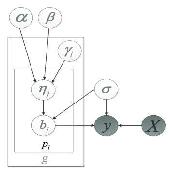
Let $I_{l}$ for $l=1,\ldots,g$ be a partition of $I=\{1,2,\ldots,p\}$; that is, $\cup_{j=1}^{g}I_{j}=I$ and $I_{j}\cap I_{l}=\emptyset$ for $j\neq l$. Let $p_{l}$ be the cardinality of $I_{l}$, and ${\bf b}_{l}=\{b_{j}:j\in I_{l}\}$ denote the subvectors of ${\bf b}$, for $l=1,\ldots,g$. The hierarchy is then specified as

$$[{\bf y}|{\bf b},\sigma] \sim N({\bf y}|{\bf X}{\bf b},\sigma{\bf I}_{n}),$$

$$[b_{j}|\eta_{l},\sigma] \stackrel{{\scriptstyle iid}}{{\sim}}\mathsf{EP}(b_{j}|0,\sigma\eta_{l},q),j\in I_{l}$$

$$[\eta_{l}|\gamma_{l},\beta,\alpha] \stackrel{{\scriptstyle ind}}{{\sim}}\mathsf{GIG}(\eta_{l}|\gamma_{l},\beta,\alpha),l=1,\ldots,g.$$

Moreover, given $\sigma$, the ${\bf b}_{l}$ are conditionally independent. By integrating out $\eta_{l}$, the marginal density of ${\bf b}_{l}$ conditional on $\sigma$ is then

$$p({\bf b}_{l}|\sigma)=\frac{K_{\frac{\gamma_{l}q{-}p_{l}}{q}}(\sqrt{\alpha(\beta{+}\sigma^{-1}\|{\bf b}_{l}\|_{q}^{q})})}{\big{[}2^{\frac{q+1}{q}}\sigma^{\frac{1}{q}}\Gamma(\frac{q{+}1}{q})\big{]}^{p_{l}}K_{\gamma_{l}}(\sqrt{\alpha\beta})}\frac{\alpha^{p_{l}/(2q)}}{\beta^{{\gamma_{l}}/2}}\Big{[}\beta{+}\sigma^{-1}\|{\bf b}_{l}\|_{q}^{q}\Big{]}^{(\gamma_{l}q-p_{l})/(2q)},$$

which implies ${\bf b}_{l}$ is non-factorial. The posterior distribution of $\eta_{l}$ on ${\bf b}_{l}$ is then $\mathsf{GIG}(\eta_{l}|\frac{\gamma_{l}q{-}p_{l}}{q},\;\beta+\sigma^{-1}\|{\bf b}_{l}\|_{q}^{q},\;\alpha)$.

In this case, the iterative procedure for $({\bf b},\sigma)$ is given by

$${\bf b}^{(t{+}1)} =\mathop{\rm argmin}_{{\bf b}}\;({\bf y}{-}{\bf X}{\bf b})^{T}({\bf y}{-}{\bf X}{\bf b})+\sum_{l=1}^{g}w_{l}^{(t{+}1)}\|{\bf b}_{l}\|_{q}^{q},$$

$$\sigma^{(t{+}1)} =\frac{q}{qn{+}2p}\Big{\{}({\bf y}{-}{\bf X}{\bf b}^{(t{+}1)})^{T}({\bf y}{-}{\bf X}{\bf b}^{(t{+}1)})+\sum_{l=1}^{g}w_{l}^{(t{+}1)}\|{\bf b}_{l}^{(t{+}1)}\|_{q}^{q}\Big{\}},$$

where for $l=1,\ldots,g$,

$$w_{l}^{(t{+}1)}=\frac{\alpha^{1/2}}{\big{[}\beta+\|{\bf b}_{l}^{(t)}\|_{q}^{q}/\sigma^{(t)}\big{]}^{1/2}}\frac{K_{\frac{\gamma_{l}q{-}q{-}p_{l}}{q}}(\sqrt{\alpha[\beta+\|{\bf b}_{l}^{(t)}\|_{q}^{q}/\sigma^{(t)}]})}{K_{\frac{\gamma_{l}q{-}p_{l}}{q}}(\sqrt{\alpha[\beta+\|{\bf b}_{l}^{(t)}\|_{q}^{q}/\sigma^{(t)}]})}.$$

Recall that there is usually no analytic computation for $w_{l}^{(t{+}1)}$. However, setting such $\gamma_{l}$ that $\frac{\gamma_{l}q{-}p_{l}}{q}=\frac{1}{2}$ or $\frac{\gamma_{l}q{-}p_{l}}{q}=-\frac{1}{2}$ can yield an analytic computation. As a result, we have

$$w_{j}^{(t{+}1)}=\left\{\begin{array}[]{ll}\Big{[}\frac{\sigma^{(t)}\alpha}{\sigma^{(t)}\beta+\|{\bf b}_{l}^{(t)}\|_{q}^{q}}\Big{]}^{1/2}&(\gamma_{l}q{-}p_{l})/q=1/2,\\ \frac{\sigma^{(t)}+\big{[}\sigma^{(t)}\alpha(\sigma^{(t)}\beta+\|{\bf b}_{l}^{(t)}\|_{q}^{q})\big{]}^{1/2}}{\sigma^{(t)}\beta+\|{\bf b}_{l}^{(t)}\|_{q}^{q}}&(\gamma_{l}q{-}p_{l})/q=-1/2.\end{array}\right.$$

Figure 3 depicts the hierarchical models in Section 4.1 and 4.2. It is clear that when $g=p$ and $p_{1}=\cdots=p_{g}=1$, the models are identical.

(a) independent

(b) grouped

Figure 3: Graphical representations.

4.3 Extensions to Logistic Regression

Another extension is the application in the penalized logistic regression model for classification. We consider a binary classification problem in which $y\in\{0,1\}$ now represents the label of the corresponding input vector ${\bf x}$. In the logistic regression model the expected value of $y_{i}$ is given by

$$P(y_{i}=1|{\bf x}_{i})=\frac{1}{1+\exp(-{\bf x}_{i}^{T}{\bf b})}\triangleq\pi_{i}.$$

In this case $\sigma=1$ and the log-likelihood function on the training data becomes

$$\log p({\bf y}|{\bf b})=\sum_{i=1}^{n}[y_{i}\log\pi_{i}+(1{-}y_{i})\log(1{-}\pi_{i})].$$

Given the $t$th estimate ${\bf b}^{(t)}$ of ${\bf b}$, the E-step of EM calculates

$$Q({\bf b}|{\bf b}^{(t)}) \triangleq\log p({\bf y}|{\bf b})+\sum_{j=1}^{p}\int{\log p[b_{j}|\eta_{j}]p(\eta_{j}|b_{j}^{(t)},\alpha,\beta,\gamma)}d\eta_{j}$$

$$\propto\sum_{i=1}^{n}[y_{i}\log\pi_{i}+(1{-}y_{i})\log(1{-}\pi_{i})]-\frac{1}{2}\sum_{j=1}^{p}w_{j}^{(t{+}1)}|b_{j}|^{q}.$$

As for the M-step, a feasible approach is to first obtain a quadratic approximation to the log-likelihood function based on its second-order Taylor series expansion at the current estimate ${\bf b}^{(t)}$ of the regression vector ${\bf b}$. We accordingly formulate a penalized linear regression model. In particular, the M-step solves the following optimization problem

$${\bf b}^{(t{+}1)}=\mathop{\rm argmin}_{{\bf b}\in{\mathbb{R}}^{p}}\;(\tilde{{\bf y}}{-}{\bf X}{\bf b})^{T}{\bf W}(\tilde{{\bf y}}{-}{\bf X}{\bf b})+\sum_{j=1}^{p}w_{j}^{(t{+}1)}|b_{j}|^{q},$$

where $\tilde{{\bf y}}$, the working response, is defined by $\tilde{{\bf y}}={\bf X}{\bf b}^{(t)}+{\bf W}^{-1}({\bf y}-\mbox{\boldmath$\pi$\unboldmath})$, ${\bf W}$ is a diagonal matrix with diagonal elements $\pi_{i}(1-\pi_{i})$, and $\mbox{\boldmath$\pi$\unboldmath}=(\pi_{1},\ldots,\pi_{n})^{T}$. Note that here the $\pi$ are evaluated at ${\bf b}^{(t)}$.

5 Iteratively Re-weighted $\ell_{q}$ Methods

We employ a penalty induced from the EP-GIG prior $\mathsf{EGIG}(b|\alpha_{0},\beta_{0},\gamma,q)$. Then the penalized regression problem is

$$\min_{{\bf b}}\;\frac{1}{2}({\bf y}{-}{\bf X}{\bf b})^{T}({\bf y}{-}{\bf X}{\bf b})-\lambda\sum_{j=1}^{p}\Big{\{}\log K_{\frac{\gamma q{-}1}{q}}(\sqrt{\alpha_{0}(\beta_{0}{+}|b_{j}|^{q})})-\frac{\gamma q{-}1}{2q}\log(\beta_{0}{+}|b_{j}|^{q})\Big{\}},$$

which can be solved via the iteratively re-weighted $\ell_{q}$ method. Given the $t$th estimate ${\bf b}^{(t)}$ of ${\bf b}$, the method considers the first Taylor approximation of $-\log\mathsf{EGIG}(b_{j}|\alpha_{0},\beta_{0},\gamma,q)$ w.r.t. $|b_{j}|^{q}$ at $|b_{j}^{(t)}|^{q}$ and solves the following problem

$$\min_{{\bf b}}\;\frac{1}{2}({\bf y}{-}{\bf X}{\bf b})^{T}({\bf y}{-}{\bf X}{\bf b})+\lambda\sum_{j=1}^{p}\omega_{j}^{(t+1)}|b_{j}|^{q},$$

where $\omega_{j}^{(t+1)}=\frac{\partial-\log\mathsf{EGIG}(b_{j}|\alpha_{0},\beta_{0},\gamma,q)}{\partial|b_{j}|^{q}}|_{b_{j}=b_{j}^{(t)}}$. It follows from Theorem 9-(ii) that

$$\omega_{j}=\frac{1}{2}\frac{\sqrt{\alpha_{0}}}{\sqrt{\beta_{0}+|b_{j}|^{q}}}\frac{K_{\frac{\gamma q-1}{q}-1}(\sqrt{\alpha_{0}(\beta_{0}+|b_{j}|^{q})})}{K_{\frac{\gamma q{-}1}{q}}(\sqrt{\alpha_{0}(\beta_{0}{+}|b_{j}|^{q})})}.$$ (11)

5.1 Relationship between EM and Iteratively Re-weighted Methods

We investigate the relationship of the EM algorithm with an iteratively re-weighted $\ell_{q}$ method where $q=1$ or $q=2$. When equating $\alpha_{0}=\alpha/\sigma$, $\beta_{0}=\beta\sigma$ and $\lambda=\sigma$, we immediately see that the $2\omega_{j}$ are equal to the $w_{j}$ in (10). This implies the iteratively re-weighted minimization method is identical to the EM algorithm given in Section 4.1.

When $q=2$, the EM algorithm is identical to the re-weighted $\ell_{2}$ method and corresponds to a local quadratic approximation (Fan and Li, 2001, Hunter and Li, 2005). And when $q=1$, the EM algorithm is the re-weighted $\ell_{1}$ minimization and corresponds to a local linear approximation (Zou and Li, 2008). Especially, when we set $\gamma=1$ and $q=2$, the EM algorithm is the same as one studied by Daubechies et al. (2010). This implies that the re-weighted $\ell_{2}$ method of Daubechies et al. (2010) can be equivalently viewed as an EM based on our proposed EP-GIG in Example 5 of Appendix B. When the EM algorithm is based on our proposed EP-GIG prior in Example 4 of Appendix B (i.e. $\gamma=1$ and $q=2$), it is then the combination of the re-weighted $\ell_{2}$ method of Daubechies et al. (2010) and the re-weighted $\ell_{2}$ method of Chartrand and Yin (2008).

When $\gamma=\frac{3}{2}$ and $q=1$, the EM algorithm (see Table 1) is equivalent to a re-weighted $\ell_{1}$ method, which in turn has a close connection with the re-weighted $\ell_{2}$ method of Daubechies et al. (2010). Additionally, the EM algorithm based on $\gamma=\frac{1}{2}$ and $q=1$ (see Table 1) can be regarded as the combination of the above re-weighted $\ell_{1}$ method and the re-weighted $\ell_{1}$ of Candès et al. (2008). Interestingly, the EM algorithm based on the EP-GIG priors given in Examples 7 and 8 of Appendix B (i.e., $\gamma=\frac{3}{2}$ and $q=\frac{1}{2}$ or $\gamma=\frac{5}{2}$ and $q=\frac{1}{2}$) corresponds a re-weighted $\ell_{1/2}$ method.

In is also worth mentioning that in Appendix C we present EP-Jeffreys priors. Using this prior, we can establish the close relationship of the adaptive lasso of Zou (2006) with an EM algorithm. In particular, when $q=1$, the EM algorithm based on the Jeffreys prior is equivalent to the adaptive lasso.

5.2 Oracle Properties

We now study the oracle property of our sparse estimator based on Laplace scale mixture priors. For this purpose, following the setup of Zou and Li (2008), we assume two conditions: (1) $y_{i}={\bf x}_{i}^{T}{\bf b}^{*}+\epsilon_{i}$ where $\epsilon_{1},\ldots,\epsilon_{n}$ are i.i.d errors with mean 0 and variance $\sigma^{2}$; (2) ${\bf X}^{T}{\bf X}/n\rightarrow{\bf C}$ where ${\bf C}$ is a positive definite matrix. Let ${\cal A}=\{j:b_{j}^{*}\neq 0\}$. Without loss of generality, we assume that ${\mathcal{A}}=\{1,2,\ldots,p_{0}\}$ with $p_{0}<p$. Thus, partition ${\bf C}$ as

$$\begin{bmatrix}{\bf C}_{11}&{\bf C}_{12}\\ {\bf C}_{21}&{\bf C}_{22}\end{bmatrix},$$

where ${\bf C}_{11}$ is $p_{0}{\times}p_{0}$. Additionally, let ${\bf b}^{*}_{1}=\{b^{*}_{j}:j\in{\mathcal{A}}\}$ and ${\bf b}^{*}_{2}=\{u_{nj}:j\notin{\cal A}\}$.

We in particular consider the following one-step sparse estimator:

$${\bf b}_{n}^{(1)}=\mathop{\rm argmin}_{{\bf b}}\;({\bf y}{-}{\bf X}{\bf b})^{T}({\bf y}{-}{\bf X}{\bf b})+\lambda_{n}\sum_{j=1}^{p}|b_{j}|\frac{Q_{\gamma{-}1}(\alpha_{n}(\beta_{n}+|b^{(0)}_{j}|))}{Q_{\gamma{-}1}(\alpha_{n}(\beta_{n}+1))},$$ (12)

where $Q_{\nu}(z)=K_{\nu-1}(\sqrt{z})/(\sqrt{z}K_{v}(\sqrt{z}))$ and ${\bf b}^{(0)}=(b_{1}^{(0)},\ldots,b_{p}^{(0)})^{T}$ is a root-$n$-consistent estimator to ${\bf b}^{*}$. The following theorem shows that this estimator has the oracle property. That is,

Theorem 11

Let ${\bf b}_{n1}^{(1)}=\{b_{nj}^{(1)}:j\in{\mathcal{A}}\}$ and ${\cal A}_{n}=\{j:b_{nj}^{(1)}\neq 0\}$. Suppose that $\lambda_{n}\rightarrow\infty$, $\lambda_{n}/\sqrt{n}\rightarrow 0$, $\alpha_{n}/{n}\rightarrow c_{1}$ and $\alpha_{n}\beta_{n}\rightarrow c_{2}$, or that $\lambda_{n}/n^{1/4}\rightarrow\infty$, $\lambda_{n}/\sqrt{n}\rightarrow 0$, $\alpha_{n}/\sqrt{n}\rightarrow c_{1}$ and $\alpha_{n}\beta_{n}\rightarrow c_{2}$. Here $c_{1},c_{2}\in(0,\infty)$. Then ${\bf b}_{n}^{(1)}$ satisfies the following properties:

1. Consistency in variable selection: $\lim_{n\rightarrow\infty}P({\cal A}_{n}={\cal A})=1$.

2. Asymptotic normality: $\sqrt{n}({\bf b}^{(1)}_{n1}-{\bf b}^{*}_{1})\rightarrow_{d}N(0,\sigma^{2}{\bf C}_{11}^{-1})$.

6 Experimental Studies

In this paper our principal purpose has been to provide a new hierarchical framework within which we can construct sparsity-inducing priors and EM algorithms. In this section we conduct an experimental investigation of particular instances of these EM algorithms. In particular, we study the cases in Table 1. We also performed two EM algorithms based on the generalized $t$ priors, i.e. the exponential power-inverse gamma priors (see Section 3.1). For simplicity of presentation, we denote them by “Method 1,” “Method 2,” “Method 3,” “Method 4,” “Method 5,” “Method 6,” and “Method 7,” respectively. Table 2 lists their EP-GIG prior setups (the notation is the same as in Section 3). As we see, using the EP-GIG priors given in Examples 7 and 8 (see Appendix B) yields EM algorithms with closed-form E-steps. However, the corresponding M-steps are a weighted $\ell_{1/2}$ minimization problem, which is not efficiently solved. Thus, we did not implement such EM algorithms.

For “Method 1,” “Method 2,” “Method 3,” “Method 5” and “Method 6,” we fix $\alpha=1$ and $\sigma^{(0)}=1$, and use the cross validation method to select $\beta$. In “Method 4” and “Method 7,” the parameter $\lambda$ was selected by using cross validation. In addition, we implemented the lasso, the adaptive lasso (adLasso) and the SCAD-based method for comparison. For the lasso, the adLasso and the re-weighted $\ell_{1}$ problems in the M-step, we solved the optimization problems by a coordinate descent algorithm (Mazumder et al., 2011).

Table 2: The EP-GIG setups of the algorithms.

Method 1	Method 2	Method 3	Method 4
$\mathsf{EGIG}(b|\sigma^{-1},\sigma\beta,\frac{1}{2},1)$	$\mathsf{EGIG}(b|\sigma^{-1},\sigma\beta,\frac{3}{2},1)$	$\mathsf{EGIG}(b|\sigma^{-1},\sigma\beta,-\frac{1}{2},1)$	$\mathsf{GT}(b|0,\frac{\sigma}{\lambda},\frac{1}{2},1)$
($q=1$, $\gamma=\frac{1}{2}$)	($q=1$, $\gamma=\frac{3}{2}$)	($q=1$, $\gamma=-\frac{1}{2}$)	($q=1$, $\tau=1$)
Method 5	Method 6	Method 7	AdLasso
$\mathsf{EGIG}(b|\sigma^{-1},\sigma\beta,0,2)$	$\mathsf{EGIG}(b|\sigma^{-1},\sigma\beta,1,2)$	$\mathsf{GT}(b|0,\frac{\sigma}{\lambda},\frac{1}{2},2)$	$\propto\exp(-|b|^{1/2})$
($q=2$, $\gamma=0$)	($q=2$, $\gamma=1$)	($q=2$, $\tau=1$)	($q=\frac{1}{2}$)

Recall that “Method 1,” “Method 2,” “Method 3,” “Method 4” and AdLasso in fact work with the nonconvex penalties. Especially, “Method 1,” “Method 2” and “Method 3” are based on the Laplace scale mixture priors proposed in Appendix B by us. “Method 4” is based on the GDP prior by Armagan et al. (2011) and Lee et al. (2010), and we employed the $\ell_{1/2}$ penalty in the adLasso. Thus, this adLasso is equivalent to the EM algorithm which given in Appendix D. Additionally, “Method 5” and “Method 6” are based on the Gaussian scale mixture priors given in Appendix B by us, and “Method 7” is based on the Cauchy prior. In Appendix C we present the EM algorithm based on the EP-Jeffreys prior. This algorithm can be also regarded as an adaptive lasso with weights $1/|b_{j}^{(t)}|$. Since the performance of the algorithms is same to that of “Method 4”, here we did not include the results with the the EP-Jeffreys prior. We also did not report the results with the Gaussian scale mixture given in Example 6 of Appendix B, because they are almost identical to those with ‘Method 5” or “Method 6”.

6.1 Reconstruction on Simulation data

We first evaluate the performance of each method on the simulated data which were used in Fan and Li (2001), Zou (2006). Let ${{\bf b}}=(3,1.5,0,0,2,0,0,0)^{T}$, ${\bf x}_{i}\stackrel{{\scriptstyle iid}}{{\sim}}N({\bf 0},\mbox{\boldmath$\Sigma$\unboldmath})$ with $\Sigma_{ij}={0.5}^{|i-j|}$, and ${\bf y}_{0}={{\bf X}}{{\bf b}}$. Then Gaussian noise ${\mbox{\boldmath$\epsilon$\unboldmath}}\sim{N}({\bf 0},\delta^{2}{\bf I}_{n})$ is added to ${\bf y}_{0}$ to form the output vector ${{\bf y}}={{\bf y}_{0}}+{\mbox{\boldmath$\epsilon$\unboldmath}}$. Let ${\hat{{\bf b}}}$ denote the sparse solution obtained from each method which takes ${\bf X}$ and ${\bf y}$ as inputs and outputs. Mean square error (MSE) $\|{\bf y}_{0}-{\bf X}\hat{{\bf b}}\|_{2}^{2}/n$ is used to measure reconstruction accuracy, and the number of zeros in $\hat{{\bf b}}$ is employed to evaluate variable selection accuracy. If a method is accurate, the number of “correct” zeros should be $5$ and “incorrect” (IC) should be $0$.

For each pair ($n$, $\delta$), we generate 10,000 datasets. In Table 3 we report the numbers of correct and incorrect zeros as well as the average and standard deviation of MSE on the 10,000 datasets. From Table 3 we see that the nonconvex penalization methods (Methods 1, 2, 3 and 4) yield the best results in terms of reconstruction accuracy and sparsity recovery. It should be pointed out that since the weights are defined as the $1/|b_{j}^{(t)}|^{1/2}$ in the adLasso method, the method suffers from numerical instability. In addition, Methods 5, 6 and 7 are based on the re-weighted $\ell_{2}$ minimization, so they do not naturally produce sparse estimates. To achieve sparseness, they have to delete small coefficients.

Table 3: Results on the simulated data sets.

	MSE($\pm$STD)	C	IC	MSE ($\pm$STD)	C	IC	MSE ($\pm$STD)	C	IC
	$n=60$, $\delta=3$			$n=120$, $\delta=3$			$n=120$, $\delta=1$
Method 1	0.699($\pm$0.63)	4.66	0.08	0.279($\pm$0.26)	4.87	0.01	0.0253($\pm$ 0.02)	5.00	0.00
Method 2	0.700($\pm$0.63)	4.55	0.07	0.287($\pm$0.30)	4.83	0.02	0.0256($\pm$0.03)	4.99	0.00
Method 3	0.728($\pm$0.60)	4.57	0.08	0.284($\pm$0.28)	4.93	0.00	0.0253($\pm$0.02)	5.00	0.00
Method 4	0.713($\pm$0.68)	4.78	0.12	0.281($\pm$0.26)	4.89	0.01	0.0255($\pm$0.03)	5.00	0.00
Method 5	1.039($\pm$0.56)	0.30	0.00	0.539($\pm$0.28)	0.26	0.00	0.0599($\pm$0.03)	0.77	0.00
Method 6	0.745($\pm$0.66)	1.36	0.00	0.320($\pm$0.26)	1.11	0.00	0.0262($\pm$0.02)	4.96	0.00
Method 7	0.791($\pm$0.57)	0.20	0.00	0.321($\pm$0.28)	0.42	0.00	0.0265($\pm$0.02)	2.43	0.00
SCAD	0.804($\pm$0.59)	3.24	0.02	0.364($\pm$0.30)	3.94	0.00	0.0264($\pm$0.03)	4.95	0.00
AdLasso	0.784($\pm$0.57)	3.60	0.04	0.335($\pm$0.27)	4.83	0.01	0.0283($\pm$0.02)	4.82	0.00
Lasso	0.816($\pm$0.53)	2.48	0.00	0.406($\pm$0.26)	2.40	0.00	0.0450($\pm$0.03)	2.87	0.00
Ridge	1.012($\pm$0.50)	0.00	0.00	0.549($\pm$0.27)	0.00	0.00	0.0658($\pm$0.03)	0.00	0.00

6.2 Regression on Real Data

We apply the methods to linear regression problems and evaluate their performance on three data sets: Pyrim and Triazines (both obtained from UCI Machine Learning Repository) and the biscuit dataset (the near-infrared (NIR) spectroscopy of biscuit doughs) (Breiman and Friedman, 1997). For Pyrim and Triazines datasets, we randomly held out 70% of the data for training and the rest for test. We repeat this process 10 times, and report the mean and standard deviation of the relative errors defined as

$$\frac{1}{n_{test}}\sum_{i=1}^{n_{test}}\left|\frac{y({\bf x}_{i}){-}\tilde{y}({\bf x}_{i})}{y({\bf x}_{i})}\right|,$$

where $y({\bf x}_{i})$ is the target output of the test input ${\bf x}_{i}$, and $\tilde{y}({\bf x}_{i})$ is the prediction value computed from a regression method. For the NIR dataset, we use the supplied training and test sets: 39 instances for training and the rest 31 for test (Breiman and Friedman, 1997). Since each response of the NIR data includes 4 attributes (“fat,” “sucrose,” “flour” and “water”), we treat the data as four regression datasets; namely, the input instances and each-attribute responses constitute one dataset.

The results are listed in Table 4. We see that the four new methods outperform the adaptive lasso and lasso in most cases. In particular Methods 1, 2, 3 and 4 (the nonconvex penalization) yield the best performance over the first two datasets, and Methods 5, 6 and 7 are the best on the NIR datasets.

Table 4: Relative error of each method on the three data sets. The numbers of instances ($n$) and numbers of features ($p$) of each data set are: $n=74$ and $p=27$ in Pyrim, $n=186$ and $p=60$ in Triazines, and $n=70$ and $p=700$ in NIR.

	Pyrim	Triazines	NIR(fat)	NIR(sucrose)	NIR(flour)	NIR(water)
Method 1	0.1342($\pm$0.065)	0.2786($\pm$0.083)	0.0530	0.0711	0.0448	0.0305
Method 2	0.1363($\pm$0.066)	0.2704($\pm$0.075)	0.0556	0.0697	0.0431	0.0312
Method 3	0.1423($\pm$0.072)	0.2792($\pm$0.081)	0.0537	0.0803	0.0440	0.0319
Method 4	0.1414($\pm$0.065)	0.2772($\pm$0.081)	0.0530	0.0799	0.0448	0.0315
Method 5	0.1381($\pm$0.065)	0.2917($\pm$0.089)	0.0290	0.0326	0.0341	0.0210
Method 6	0.2352($\pm$0.261)	0.3364($\pm$0.079)	0.0299	0.0325	0.0341	0.0208
Method 7	0.1410($\pm$0.065)	0.3109($\pm$0.110)	0.0271	0.0423	0.0277	0.0279
SCAD	0.1419($\pm$0.064)	0.2807($\pm$0.079)	0.0556	0.0715	0.0467	0.0352
AdLasso	0.1430($\pm$0.064)	0.2883($\pm$0.080)	0.0533	0.0803	0.0486	0.0319
Lasso	0.1424($\pm$0.064)	0.2804($\pm$0.079)	0.0608	0.0799	0.0527	0.0340

6.3 Experiments on Group Variable Selection

Here we use $p=32$ with $8$ groups, each of size $4$. Let $\mbox{\boldmath$\beta$\unboldmath}_{1:4}=(3,1.5,2,0.5)^{T}$, $\mbox{\boldmath$\beta$\unboldmath}_{9:12}=\mbox{\boldmath$\beta$\unboldmath}_{17:20}=(6,3,4,1)^{T}$, $\mbox{\boldmath$\beta$\unboldmath}_{25:28}=(1.5,0.75,1,0.25)^{T}$ with all other entries set to zero, while ${\bf X}$, ${\bf y}_{0}$, and ${\bf y}$ are defined in the same way as in Section 6.1. If a method is accurate, the number of “correct” zeros should be $16$ and “incorrect” (IC) should be $0$. Results are reported in Table 5.

Table 5: Results on the simulated data sets.

	MSE($\pm$STD)	C	IC	MSE ($\pm$STD)	C	IC	MSE ($\pm$STD)	C	IC
	$n=60$, $\delta=3$			$n=120$, $\delta=3$			$n=120$, $\delta=1$
Method $1^{\prime}$	2.531($\pm$1.01)	15.85	0.31	1.201($\pm$0.45)	16.00	0.14	0.1335($\pm$0.048)	15.72	0.01
Method $2^{\prime}$	2.516($\pm$1.06)	15.87	0.28	1.200($\pm$0.43)	15.97	0.10	0.1333($\pm$0.047)	15.87	0.00
Method $3^{\prime}$	2.445($\pm$0.96)	15.88	0.54	1.202($\pm$0.43)	15.98	0.25	0.1301($\pm$0.047)	16.00	0.01
Method $4^{\prime}$	2.674($\pm$1.12)	15.40	0.30	1.220($\pm$0.45)	15.79	0.49	0.1308($\pm$0.047)	16.00	0.00
Method $5^{\prime}$	2.314($\pm$0.90)	5.77	0.04	1.163($\pm$0.41)	7.16	0.03	0.1324($\pm$0.047)	16.00	0.01
Method $6^{\prime}$	2.375($\pm$0.92)	10.18	0.04	1.152($\pm$0.41)	15.56	0.03	0.1322($\pm$0.047)	16.00	0.00
Method $7^{\prime}$	2.478($\pm$0.97)	9.28	0.05	1.166($\pm$0.41)	14.17	0.03	0.1325($\pm$0.047)	15.96	0.00
glasso	2.755($\pm$0.92)	5.52	0.00	1.478($\pm$0.48)	3.45	0.00	0.1815($\pm$0.058)	3.05	0.00
AdLasso	3.589($\pm$1.10)	11.36	2.66	1.757($\pm$0.56)	11.85	1.42	0.1712($\pm$0.058)	14.09	0.32
Lasso	3.234($\pm$0.99)	9.17	1.29	1.702($\pm$0.52)	8.53	0.61	0.1969($\pm$0.060)	8.03	0.05

6.4 Experiments on Classification

In this subsection we apply our hierarchical penalized logistic regression models in Section 4.3 to binary classification problems over five real-world data sets: Ionosphere, Spambase, Sonar, Australian, and Heart from UCI Machine Learning Repository and Statlog. Table 6 gives a brief description of these five datasets.

Table 6: The description of datasets. Here $n$: the numbers of instances; $p$: the numbers of features.

	Ionosphere	Spambase	Sonar	Australian	Heart
$n$	$351$	$4601$	$208$	$690$	$270$
$p$	$33$	$57$	$60$	$14$	$13$

In the experiments, the input matrix ${\bf X}\in{\mathbb{R}}^{n\times p}$ is normalized such that $\sum_{i=1}^{n}x_{ij}=0$ and $\sum_{i=1}^{n}x_{ij}^{2}=n$ for all $j=1,\cdots,p$. For each data set, we randomly choose 70% for training and the rest for test. We repeat this process 10 times and report the mean and the standard deviation of classification error rate. The results in Table 7 are encouraging, because in most cases Methods 1, 2, 3 and 4 based on the nonconvex penalties perform over the other methods in both accuracy and sparsity.

Table 7: Misclassification rate (%) of each method on the five data sets.

	Ionosphere	Spambase	Sonar	Australian	Heart
Method 1	9.91($\pm$2.19)	7.54($\pm$0.84)	18.71($\pm$5.05)	12.46($\pm$2.08)	13.83($\pm$3.33)
Method 2	10.19($\pm$2.03)	7.47($\pm$0.85)	19.19($\pm$5.18)	12.56($\pm$2.06)	14.20($\pm$3.50)
Method 3	10.00($\pm$1.95)	7.58($\pm$0.83)	19.03($\pm$4.35)	12.61($\pm$2.15)	14.32($\pm$3.60)
Method 4	10.66($\pm$1.94)	7.61($\pm$0.83)	21.65($\pm$5.11)	12.65($\pm$2.14)	13.95($\pm$3.49)
Method 5	11.51($\pm$3.77)	8.78($\pm$0.41)	21.61($\pm$5.70)	12.03($\pm$1.74)	13.21($\pm$3.14)
Method 6	11.51($\pm$3.72)	8.86($\pm$0.41)	21.94($\pm$5.85)	13.24($\pm$2.22)	14.57($\pm$3.38)
Method 7	11.70($\pm$4.06)	9.49($\pm$0.33)	22.58($\pm$5.84)	14.11($\pm$2.48)	13.46($\pm$3.10)
SCAD	10.47($\pm$2.06)	7.58($\pm$0.83	21.94($\pm$5.60)	12.66($\pm$2.08)	13.83($\pm$3.43)
$\ell_{{1}/{2}}$	10.09($\pm$1.67)	7.51($\pm$0.86)	20.00($\pm$5.95)	12.56($\pm$2.15)	14.20($\pm$3.78)
$\ell_{1}$	10.47($\pm$1.96)	7.57($\pm$0.83)	21.61($\pm$5.11)	12.66($\pm$2.15)	13.95($\pm$3.49)

7 Conclusions

In this paper we have proposed a family of sparsity-inducing priors that we call exponential power-generalized inverse Gaussian (EP-GIG) distributions. We have defined EP-GIG as a mixture of exponential power distributions with a generalized inverse Gaussian (GIG) density. EP-GIG are extensions of Gaussian scale mixtures and Laplace scale mixtures. As a special example of the EP-GIG framework, the mixture of Laplace with GIG can induce a family of nonconvex penalties. In Appendix B, we have especially presented five now EP-GIG priors which can induce nonconvex penalties.

Since GIG distributions are conjugate with respect to the exponential power distribution, EP-GIG are natural for Bayesian sparse learning. In particular, we have developed hierarchical Bayesian models and devised EM algorithms for finding sparse solutions. We have also shown how this framework can be applied to grouped variable selection and logistic regression problems. Our experiments have validate that our proposed EP-GIG priors forming nonconvex penalties are potentially feasible and effective in sparsity modeling.

A Proofs

In order to obtain proofs, we first present some mathematical preliminaries that will be needed.

A.1 Mathematical Preliminaries

The first three of the following lemmas are well known, so we omit their proofs.

Lemma 12

Let $\lim_{\nu\rightarrow\infty}\;a(\nu)=a$. Then $\lim_{\nu\rightarrow\infty}\;\left(1+\frac{a(\nu)}{\nu}\right)^{\nu}=\exp(a)$.

Lemma 13

(Stirling Formula) $\lim_{\nu\rightarrow\infty}\frac{\Gamma(\nu)}{(2\pi)^{1/2}\nu^{\nu-1/2}\exp(-\nu)}=1$.

Lemma 14

Assume $z>0$ and $\nu>0$. Then

$$\lim_{\nu\rightarrow\infty}\frac{K_{\nu}(\nu^{1/2}z)}{\pi^{1/2}2^{\nu{-}1/2}\nu^{(\nu-1)/2}z^{-\nu}\exp(-\nu)\exp(-z^{2}/4)}=1.$$

ProofT Consider the integral representation of $K_{\nu}(\nu^{1/2}z)$ as

$$K_{\nu}(\nu^{1/2}z) =\pi^{-1/2}2^{\nu}\nu^{\nu/2}z^{\nu}\Gamma\big{(}\nu+\frac{1}{2}\big{)}\int_{0}^{\infty}{(t^{2}+\nu z^{2})^{-\nu-\frac{1}{2}}\cos(t)dt}$$

$$=\pi^{-1/2}2^{\nu}\nu^{-(\nu+1)/2}z^{-(\nu{+}1)}\Gamma\big{(}\nu+\frac{1}{2}\big{)}\int_{0}^{\infty}{\frac{\cos(t)}{(1+t^{2}/(\nu z^{2}))^{\nu+\frac{1}{2}}}\cos(t)dt}.$$

Thus, we have

$$\lim_{\nu\rightarrow\infty}\frac{K_{\nu}(\nu^{1/2}z)}{\pi^{-1/2}2^{\nu}\nu^{-(\nu+1)/2}z^{-(\nu{+}1)}\Gamma\big{(}\nu+\frac{1}{2}\big{)}} =\lim_{\nu\rightarrow\infty}\int_{0}^{\infty}{\frac{\cos(t)}{(1+t^{2}/(\nu z^{2}))^{\nu+\frac{1}{2}}}\cos(t)dt}$$

$$=\int_{0}^{\infty}{\cos(t)\exp(-t^{2}/z^{2})dt}.$$

We now calculate the integral $\int_{0}^{\infty}{\cos(t)\exp(-t^{2}/z^{2})dt}$ for $z>0$. We denote this integral by $\phi(z)$ and let $u=t/z$. Hence,

$$\phi(z)=z\int_{0}^{\infty}\exp(-u^{2})\cos(uz)du=zf(z)$$

where $f(z)=\int_{0}^{\infty}\exp(-u^{2})\cos(uz)du$. Note that

$$f^{\prime}(z) ={-}\int_{0}^{\infty}{\exp(-u^{2})\sin(uz)udu}=\frac{1}{2}\int_{0}^{\infty}{\sin(uz)d\exp(-u^{2})}$$

$$={-}\frac{z}{2}\int_{0}^{\infty}{\exp(-u^{2})\cos(uz)du}=-\frac{z}{2}f(z),$$

which implies that $f(z)=C\exp(-z^{2}/4)$ where $C$ is a constant independent of $z$. We calculate $f(1)$ to obtain $C$. Since

$$C=\lim_{z\rightarrow+0}f(z)=\lim_{z\rightarrow+0}\int_{0}^{\infty}e^{-u^{2}}\cos(uz)du=\int_{0}^{\infty}e^{-u^{2}}du=\frac{\sqrt{\pi}}{2},$$

we have $\phi(z)=\frac{\sqrt{\pi}}{2}z\exp(-z^{2}/4)$. Subsequently,

$$\lim_{\nu\rightarrow\infty}\frac{K_{\nu}(\nu^{1/2}z)}{\pi^{-1/2}2^{\nu}\nu^{-(\nu+1)/2}z^{-(\nu{+}1)}\Gamma\big{(}\nu+\frac{1}{2}\big{)}}=\frac{\sqrt{\pi}}{2}z\exp(-z^{2}/4).$$

On the other hand, it follows from Lemmas 12 and 13 that

$$\lim_{\nu\rightarrow\infty}\frac{\Gamma(\nu+1/2)}{(2\pi)^{1/2}\nu^{\nu}\exp(-\nu)}=\lim_{\nu\rightarrow\infty}\frac{\Gamma(\nu+1/2)}{\sqrt{2\pi}\nu^{\nu}[1{+}1/(2\nu)]^{\nu}\exp({-}\nu)\exp(-1/2)}=1.$$

Thus,

$$\lim_{\nu\rightarrow\infty}\frac{K_{\nu}(\nu^{1/2}z)}{\pi^{\frac{1}{2}}2^{\nu-\frac{1}{2}}\nu^{\frac{\nu{-}1}{2}}z^{{-}\nu}\exp(-\nu)\exp(-\frac{z^{2}}{4})}=1.$$

 

Lemma 15

The modified Bessel function of the second kind $K_{\gamma}(u)$ satisfies the following propositions:

$K_{\gamma}(u)=K_{-\gamma}(u)$;

$K_{\gamma+1}(u)=2\frac{\gamma}{u}K_{\gamma}(u)+K_{\gamma{-}1}(u)$;

$K_{1/2}(u)=K_{-1/2}(u)=\sqrt{\frac{\pi}{2u}}\exp(-u)$;

$\frac{\partial K_{\gamma}(u)}{\partial u}=-\frac{1}{2}(K_{\gamma-1}(u)+K_{\gamma+1}(u))=-K_{\gamma-1}(u)-\frac{\gamma}{u}K_{\gamma}(u)=\frac{\gamma}{u}K_{\gamma}(u)-K_{\gamma+1}(u)$.

For $\gamma\in(-\infty,+\infty)$, $K_{\gamma}(u)\sim\sqrt{\frac{\pi}{2u}}\exp(-u)$ as $u\rightarrow+\infty$.

Lemma 16

Let $Q_{\nu}(z)=K_{\nu{-}1}(\sqrt{z})/(\sqrt{z}K_{\nu}(\sqrt{z}))$ where $\nu\in{\mathbb{R}}$ and $z>0$. Then, $Q_{\nu}$ is completely monotone.

ProofT When $\nu\geq 0$, the case was well proved by Grosswald (1976). Thus, we only need to prove the case that $\nu<0$. In this case, we let $\nu=-\tau$ where $\tau>0$. Thus,

$$Q_{\nu}=\frac{K_{-\tau{-}1}(\sqrt{z})}{\sqrt{z}K_{-\tau}(\sqrt{z})}=\frac{K_{\tau{+}1}(\sqrt{z})}{\sqrt{z}K_{\tau}(\sqrt{z})}=\frac{2\tau}{z}+\frac{K_{\tau{-}1}(\sqrt{z})}{\sqrt{z}K_{\tau}(\sqrt{z})},$$

which is obvious completely monotone.  

The following proposition of the GIG distribution can be found from Jørgensen (1982).

Proposition 17

Let $\eta$ be distributed according to ${\mathsf{GIG}}(\eta|\gamma,\beta,\alpha)$ with $\alpha>0$ and $\beta>0$. Then

$$E(\eta^{\nu})=\Big{(}\frac{\beta}{\alpha}\Big{)}^{\nu/2}\frac{K_{\gamma+\nu}(\sqrt{\alpha\beta})}{K_{\gamma}(\sqrt{\alpha\beta})}.$$

We are especially interested in the cases that $\gamma=1/2$, $\gamma=-1/2$, $\gamma=3/2$ and $\gamma=-3/2$. For these cases, we have the following results.

Proposition 18

Let $\alpha>0$ and $\beta>0$.

1. If $\eta$ is distributed according to ${\mathsf{GIG}}(\eta|1/2,\beta,\alpha)$, then

   $$E(\eta)=\frac{1+\sqrt{\alpha\beta}}{\alpha},\quad E(\eta^{-1})=\sqrt{\frac{\alpha}{\beta}}.$$

2. If $\eta$ is distributed according to ${\mathsf{GIG}}(\eta|{-}1/2,\beta,\alpha)$, then

   $$E(\eta)=\sqrt{\frac{\beta}{\alpha}},\quad E(\eta^{-1})=\frac{1+\sqrt{\alpha\beta}}{\beta}.$$

3. If $\eta$ is distributed according to ${\mathsf{GIG}}(\eta|3/2,\beta,\alpha)$, then

   $$E(\eta)=\frac{3}{\alpha}+\frac{\beta}{1+\sqrt{\alpha\beta}},\quad E(\eta^{-1})=\frac{\alpha}{1+\sqrt{\alpha\beta}}.$$

4. If $\eta$ is distributed according to ${\mathsf{GIG}}(\eta|{-}3/2,\beta,\alpha)$, then

   $$E(\eta)=\frac{\beta}{1+\sqrt{\alpha\beta}},\quad E(\eta^{-1})=\frac{3}{\beta}+\frac{\alpha}{1+\sqrt{\alpha\beta}}.$$

ProofT It follows from Lemma 15 that $K_{3/2}(u)=\frac{1{+}u}{u}K_{1/2}(u)=\frac{1{+}u}{u}K_{-1/2}(u)$.

We first consider the case that $\eta\sim\mathsf{GIG}(\eta|1/2,\beta,\alpha)$. Consequently, $E(\eta^{-1})=\alpha/\beta$ and

$$E(\eta)=\Big{(}\frac{\beta}{\alpha}\Big{)}^{1/2}\frac{K_{\frac{3}{2}}(\sqrt{\alpha\beta})}{K_{\frac{1}{2}}(\sqrt{\alpha\beta})}=\Big{(}\frac{\beta}{\alpha}\Big{)}^{1/2}\frac{1+\sqrt{\alpha\beta}}{\sqrt{\alpha\beta}}=\frac{1+\sqrt{\alpha\beta}}{\alpha}.$$

As for the case that $\eta\sim\mathsf{GIG}(\eta|{-}3/2,\beta,\alpha)$, it follows from Proposition 17 that

$$E(\eta)=\Big{(}\frac{\beta}{\alpha}\Big{)}^{1/2}\frac{K_{-1/2}(\sqrt{\alpha\beta})}{K_{-3/2}(\sqrt{\alpha\beta})}=\frac{\beta}{1+\sqrt{\alpha\beta}}$$

and

$$E(\eta^{-1})=\Big{(}\frac{\beta}{\alpha}\Big{)}^{-1/2}\frac{K_{-5/2}(\sqrt{\alpha\beta})}{K_{-3/2}(\sqrt{\alpha\beta})}=\frac{3}{\beta}+\frac{\alpha}{1+\sqrt{\alpha\beta}}.$$

Likewise, we have the second and third parts.  

A.2 The Proof of Proposition 1

Note that

$$\lim_{\tau\rightarrow\infty}G(\eta|\tau,\tau\lambda) =\lim_{\tau\rightarrow\infty}\frac{(\tau\lambda)^{\tau}}{\Gamma(\tau)}\eta^{\tau-1}\exp(-\tau\lambda\eta)$$

$$=\lim_{\tau\rightarrow\infty}\frac{(\tau\lambda)^{\tau}}{(2\pi)^{\frac{1}{2}}\tau^{\tau-\frac{1}{2}}\exp(-\tau)}\eta^{\tau-1}\exp(-\tau\lambda\eta)\quad\mbox{(Use the Stirling Formula)}$$

$$=\lim_{\tau\rightarrow\infty}\frac{\tau^{\frac{1}{2}}}{(2\pi)^{\frac{1}{2}}\eta}\frac{(\lambda\eta)^{\tau}}{\exp((\lambda\eta-1)\tau)}.$$

Since $\ln u\leq u-1$ for $u>0$, with equality if and only if $u=1$, we can obtain the proof.

Likewise, we also have the second part.

A.3 The Proof of Proposition 2

Using Lemma 14

$$\lim_{\gamma\rightarrow+\infty}\mathsf{GIG}(\eta|\gamma,\beta,\gamma\alpha) =\lim_{\gamma\rightarrow+\infty}\frac{\gamma^{\gamma/2}(\alpha/\beta)^{\gamma/2}}{2K_{\gamma}(\sqrt{\gamma\alpha\beta})}\eta^{\gamma-1}\exp(-(\gamma\alpha\eta+\beta\eta^{-1})/2)$$

$$=\lim_{\nu\rightarrow+\infty}\frac{\alpha^{\gamma}\exp(\frac{\alpha\beta}{4})\exp(-\beta\eta^{-1}/2)}{\pi^{\frac{1}{2}}2^{\gamma{+}\frac{1}{2}}\gamma^{-\frac{1}{2}}}\eta^{\gamma-1}\exp(-\gamma(\alpha\eta/2{-}1))$$

$$=\lim_{\gamma\rightarrow+\infty}\frac{\eta^{-1}\gamma^{\frac{1}{2}}\exp(\frac{\alpha\beta}{4})}{(2\pi)^{\frac{1}{2}}\exp(\beta\eta^{-1}/2)}(\alpha\eta/2)^{\gamma}\exp(-\gamma(\alpha\eta/2{-}1))$$

$$=\delta(\eta|2/\alpha).$$

Again since $\ln u\leq u-1$ for $u>0$, with equality if and only if $u=1$, we can obtain the proof of Part (1).

Let $\tau=-\gamma$. We have

$$\lim_{\gamma\rightarrow-\infty}\mathsf{GIG}(\eta|\gamma,-\gamma\beta,\alpha) =\lim_{\tau\rightarrow+\infty}\mathsf{GIG}(\eta|-\tau,\tau\beta,\alpha)$$

$$=\lim_{\tau\rightarrow+\infty}\frac{(\alpha/(\tau\beta))^{-\tau/2}}{2K_{\tau}(\sqrt{\tau\alpha\beta})}\eta^{-\tau-1}\exp(-(\alpha\eta+\tau\beta\eta^{-1})/2)$$

due to $K_{-\tau}(\sqrt{\tau\alpha\beta})=K_{\tau}(\sqrt{\tau\alpha\beta})$. Accordingly, we also have the second part.

A.4 The Proof of Proposition 3

Based on (4) and Lemma 15, we have that

$$\lim_{\psi\rightarrow+\infty}p(\eta)=\lim_{\psi\rightarrow+\infty}\frac{\psi^{1/2}}{\sqrt{2\pi}}\frac{1}{\exp(\frac{\psi}{2\phi\eta}(\phi\eta-1)^{2})}=\delta(\eta|\phi).$$

A.5 The Proof of Theorem 4

$$p(b) =\int_{0}^{+\infty}{{\mathsf{EP}}(b|0,\eta,q){\mathsf{GIG}}(\eta|\gamma,\beta,\alpha)d\eta}$$

$$=\int_{0}^{+\infty}{\frac{\eta^{-1/q}}{2^{\frac{q+1}{q}}\Gamma(\frac{q{+}1}{q})}\exp(-\eta^{-1}|b|^{q}/2)\frac{(\alpha/\beta)^{{\gamma}/2}}{2K_{\gamma}(\sqrt{\alpha\beta})}\eta^{{\gamma}-1}\exp(-(\alpha\eta+\beta\eta^{-1})/2)d\eta}$$

$$=\frac{(\alpha/\beta)^{{\gamma}/2}}{2^{\frac{2q+1}{q}}\Gamma(\frac{q{+}1}{q})K_{\gamma}(\sqrt{\alpha\beta})}\int_{0}^{+\infty}{\eta^{\frac{\gamma q-1}{q}-1}\exp[-(\alpha\eta+(\beta+|b|^{q})\eta^{-1})/2]d\eta}$$

$$=\frac{K_{\frac{\gamma q{-}1}{q}}(\sqrt{\alpha(\beta{+}|b|^{q})})}{2^{\frac{q+1}{q}}\Gamma(\frac{q{+}1}{q})K_{\gamma}(\sqrt{\alpha\beta})}\frac{\alpha^{1/(2q)}}{\beta^{{\gamma}/2}}[\beta{+}|b|^{q}]^{(\gamma q-1)/(2q)}.$$

A.6 The Proof of Theorem 5

The proof can be directly obtained from Proposition 2. That is,

$$\lim_{\gamma\rightarrow+\infty}\mathsf{EGIG}(b|\gamma\alpha,\beta,\gamma,q) =\lim_{\gamma\rightarrow+\infty}\int{\mathsf{EP}(b|0,\gamma,q)\mathsf{GIG}(\eta|\gamma,\beta,\gamma\alpha)d\eta}$$

$$=\int{\mathsf{EP}(b|0,\gamma,q)\delta(\eta|2/\alpha)d\eta}=\mathsf{EP}(b|0,2/\alpha,q).$$

Likewise, we have the proof for the second part. As for the third part, it can be immediately obtained from Proposition 3.

A.7 The Proof of Theorem 6

Note that

$$\lim_{\tau\rightarrow\infty}\mathsf{GT}(b|u,\tau/\lambda,\tau/2,q)=\lim_{\tau\rightarrow\infty}\frac{q}{2}\frac{\Gamma(\frac{\tau}{2}{+}\frac{1}{q})}{\Gamma(\frac{\tau}{2})\Gamma(\frac{1}{q})}\Big{(}\frac{\lambda}{\tau}\Big{)}^{\frac{1}{q}}\Big{(}1+\frac{\lambda}{\tau}|b-u|^{q}\Big{)}^{-(\frac{\tau}{2}+\frac{1}{q})}.$$

It follows from Lemmas 12 and 13 that

$$\lim_{\tau\rightarrow\infty}\;\Big{(}1+\frac{\lambda}{\tau}|b-u|^{q}\Big{)}^{-(\frac{\tau}{2}+\frac{1}{q})}=\exp\left(-\frac{\lambda}{2}|b-u|^{q}\right)$$

and

$$\lim_{\tau\rightarrow\infty}\frac{q}{2}\frac{\Gamma(\frac{\tau}{2}{+}\frac{1}{q})}{\Gamma(\frac{\tau}{2})\Gamma(\frac{1}{q})}\Big{(}\frac{\lambda}{\tau}\Big{)}^{\frac{1}{q}} =\lim_{\tau\rightarrow\infty}\frac{q}{2\Gamma({1}/{q})}\Big{(}\frac{\lambda}{\tau}\Big{)}^{\frac{1}{q}}\frac{(\frac{\tau}{2}{+}\frac{1}{q})^{\frac{\tau}{2}{+}\frac{1}{q}-\frac{1}{2}}}{(\frac{\tau}{2})^{\frac{\tau-1}{2}}}\exp\Big{(}-\frac{1}{q}\Big{)}$$

$$=\lim_{\tau\rightarrow\infty}\frac{q}{2\Gamma({1}/{q})}\Big{(}\frac{\lambda}{2}+\frac{\lambda}{q\tau}\Big{)}^{1/q}\Big{(}1+\frac{2}{q\tau}\Big{)}^{\frac{\tau-1}{2}}\exp\Big{(}-\frac{1}{q}\Big{)}$$

$$=\frac{q}{2\Gamma({1}/{q})}\Big{(}\frac{\lambda}{2}\Big{)}^{1/q}.$$

Thus, the proof completes.

A.8 The Proof of Theorem 7

According to Proposition 1, we have

$$\lim_{\gamma\rightarrow\infty}\mathsf{EG}(b|\lambda\gamma,\gamma/2,q) =\lim_{\gamma\rightarrow\infty}\int_{0}^{\infty}{\mathsf{EP}(b|0,\eta,q)G(\eta|\gamma/2,\lambda\gamma/2)}d\eta$$

$$=\int_{0}^{\infty}{\mathsf{EP}(b|0,\eta,q)\big{[}\lim_{\gamma\rightarrow\infty}G(\eta|\gamma/2,\lambda\gamma/2)}\big{]}d\eta$$

$$=\int_{0}^{\infty}{\mathsf{EP}(b|0,\eta,q)\delta(\eta|1/\lambda)}d\eta$$

$$=\mathsf{EP}(b|0,1/\lambda,q).$$

A.9 The Proof of Theorem 8

With the setting that $\gamma=\frac{1}{2}+\frac{1}{q}$, we have

$$\int_{0}^{\infty}{\mathsf{EP}(b|0,\eta,q)G(\eta|\gamma,\alpha/2)}d\eta =\frac{\alpha^{\frac{1}{q}+\frac{1}{4}}|b|^{\frac{q}{4}}}{2^{\frac{2}{q}{+}\frac{1}{2}}\Gamma(\frac{q{+}1}{q})\Gamma(\frac{1}{2}+\frac{1}{q})}K_{1/2}(\sqrt{\alpha|b|^{q}})$$

$$=\frac{\alpha^{\frac{1}{q}+\frac{1}{4}}|b|^{\frac{q}{4}}}{2^{\frac{2}{q}{+}\frac{1}{2}}2^{-\frac{2}{q}}\sqrt{\pi}\frac{2}{q}\Gamma(\frac{2}{q})}\frac{2^{-1/2}\sqrt{\pi}}{(\alpha|b|^{q})^{1/4}}\exp(-\sqrt{\alpha|b|^{q}})$$

$$=\frac{q\alpha^{1/q}}{4\Gamma(\frac{2}{q})}\exp(-\sqrt{\alpha|b|^{q}})=\mathsf{EP}(b|0,\alpha^{-1/2}/2,q/2).$$

Here we use the fact that $\Gamma(\frac{q{+}1}{q})\Gamma(\frac{1}{2}{+}\frac{1}{q})=2^{1-2(\frac{1}{2}{+}\frac{1}{q})}\sqrt{\pi}\Gamma(1+\frac{2}{q})=2^{-\frac{2}{q}}\sqrt{\pi}\frac{2}{q}\Gamma(\frac{2}{q})$.

A.10 The Proof of Theorem 9

The first part is immediate. We consider the proof of the second part. It follows from Lemma 15 that

$$\frac{\partial-\log p(b)}{\partial|b|^{q}} =\frac{K_{\frac{\gamma q-1}{q}-1}(\sqrt{\alpha(\beta+|b|^{q})})+\frac{(\gamma q-1)/q}{\sqrt{\alpha(\beta+|b|^{q})}}K_{\frac{\gamma q-1}{q}}(\sqrt{\alpha(\beta+|b|^{q})})}{K_{\frac{\gamma q-1}{q}}(\sqrt{\alpha(\beta+|b|^{q})})}\frac{1}{2}\frac{\alpha}{\sqrt{\alpha(\beta+|b|^{q})}}$$

$$\quad-\frac{\gamma q-1}{2q}\frac{1}{\beta+|b|^{q}}$$

$$=\frac{1}{2}\frac{\sqrt{\alpha}}{\sqrt{\beta+|b|^{q}}}\frac{K_{\frac{\gamma q-1}{q}-1}(\sqrt{\alpha(\beta+|b|^{q})})}{K_{\frac{\gamma q-1}{q}}(\sqrt{\alpha(\beta+|b|^{q})})}=\frac{1}{2}E(\eta^{-1}|b).$$

due to that $\eta|b\sim\mathsf{GIG}(\eta|(\gamma q-1)/q,\sqrt{\beta+|b|^{q}},\alpha)$.

A.11 The Proof of Theorem 10

For notational simplicity, we let $z=|b^{q}|$, $\nu=\frac{\gamma q-1}{q}$ and $\phi(z)=\frac{\partial-\log p(b)}{\partial|b|^{q}}$. According to the above proof, we have

$$\phi(z)=\frac{\alpha}{2}\frac{1}{\sqrt{\alpha(\beta+z)}}\frac{K_{\nu-1}(\sqrt{\alpha(\beta+z)})}{K_{\nu}(\sqrt{\alpha(\beta+z)})}.$$

It then follows from Lemma 16 that $\phi(z)$ is completely monotone.

A.12 The Proof of Theorem 11

Let ${{\bf b}}_{n}^{(1)}={\bf b}^{*}+\frac{{\bf u}}{\sqrt{n}}$ and

$$\hat{{\bf u}}=\mathop{\rm argmin}_{{\bf u}}\;\bigg{\{}\Psi({\bf u}):=\Big{\|}{\bf y}-{\bf X}({\bf b}^{*}+\frac{{\bf u}}{\sqrt{n}})\Big{\|}^{2}+\lambda_{n}\sum_{j=1}^{p}\omega_{j}^{(0)}|b^{*}_{j}{+}\frac{u_{j}}{\sqrt{n}}|\bigg{\}},$$

where

$$\omega_{j}^{(0)}=\frac{\sqrt{\alpha_{n}\beta_{n}+\alpha_{n}}}{\sqrt{\alpha_{n}(\beta_{n}+|b^{(0)}_{j}|)}}\frac{K_{\gamma{-}2}(\sqrt{\alpha_{n}(\beta_{n}+|b^{(0)}_{j}|)})}{K_{\gamma{-}1}(\sqrt{\alpha_{n}(\beta_{n}{+}|b^{(0)}_{j}|)})}\frac{K_{\gamma{-}1}(\sqrt{\alpha_{n}(\beta_{n}+1))}}{K_{\gamma{-}2}(\sqrt{\alpha_{n}(\beta_{n}{+}1))}}.$$

Consider that

$$\Psi({\bf u})-\Psi(0)={\bf u}^{T}(\frac{1}{n}{\bf X}^{T}{\bf X}){\bf u}{-}2\frac{\mbox{\boldmath$\epsilon$\unboldmath}^{T}{\bf X}}{\sqrt{n}}{\bf u}{+}\lambda_{n}\sum_{j=1}^{p}\omega_{j}^{(0)}\Big{\{}\big{|}b^{*}_{j}{+}\frac{u_{j}}{\sqrt{n}}\big{|}{-}|b^{*}_{j}|\Big{\}}.$$

We know that ${\bf X}^{T}{\bf X}/n\rightarrow{\bf C}$ and $\frac{{\bf X}^{T}\mbox{\boldmath$\epsilon$\unboldmath}}{\sqrt{n}}\rightarrow_{d}N({\bf 0},\sigma^{2}{\bf C})$. We thus only consider the third term of the right-hand side of the above equation. Since $\alpha_{n}\beta_{n}\rightarrow c_{1}$ and $\alpha_{n}\rightarrow\infty$ (note that $\alpha_{n}/{n}\rightarrow c_{2}>0$ implies $\alpha_{n}\rightarrow+\infty$), we have

$$\frac{K_{\gamma{-}1}(\sqrt{\alpha_{n}(\beta_{n}+1))}}{K_{\gamma{-}2}(\sqrt{\alpha_{n}(\beta_{n}{+}1))}}\rightarrow 1.$$

If $b^{*}_{j}=0$, then $\sqrt{n}(|b^{*}_{j}+\frac{u_{j}}{\sqrt{n}}|-|b^{*}_{j}|)=|u_{j}|$. And since $\sqrt{n}b_{j}^{(0)}=O_{p}(1)$, we have $\alpha_{n}|b^{(0)}_{j}|=(\alpha_{n}/\sqrt{n})\sqrt{n}|b^{(0)}_{j}|=O_{p}(1)$. Hence, $Q_{\gamma{-}1}(\alpha_{n}(\beta_{n}+|b^{(0)}_{j}|))$ converges to a positive constant in probability. As a result, we obtain

$$\frac{\lambda_{n}\omega^{(0)}_{j}}{\sqrt{n}}\rightarrow_{p}\rightarrow\infty.$$

due to

$$\frac{\sqrt{\alpha_{n}\beta_{n}+\alpha_{n}}}{\sqrt{n}}\frac{K_{\gamma{-}1}(\sqrt{\alpha_{n}\beta_{n}+\alpha_{n}})}{K_{\gamma{-}2}(\sqrt{\alpha_{n}\beta_{n}+\alpha_{n}})}\rightarrow\sqrt{c_{2}}.$$

If $b^{*}_{j}\neq 0$, then $\omega^{(0)}_{j}\rightarrow_{p}\frac{1}{\sqrt{|b^{(0)}_{j}|}}>0$ and $\sqrt{n}(|b^{*}_{j}+\frac{u_{j}}{\sqrt{n}}|-|b^{*}_{j}|)\rightarrow u_{j}\mathrm{sgn}(b^{*}_{j})$. Thus $\lambda_{n}\frac{\omega^{(0)}_{j}}{\sqrt{n}}\sqrt{n}(|b^{*}_{j}{+}\frac{u_{j}}{\sqrt{n}}|-|b^{*}_{j}|)\rightarrow_{p}0$. The remaining parts of the proof can be immediately obtained via some slight modifications to that in Zou (2006) or Zou and Li (2008). We here omit them.

B Several Special EP-GIG Distributions

We now present eight other important concrete EP-GIG distributions, obtained from particular settings of ${\gamma}$ and $q$.

Example 1

We first discuss the case that $q=1$ and ${\gamma}=1/2$. That is, we employ the mixing distribution of $L(b|0,\eta)$ with ${\mathsf{GIG}}(\eta|1/2,\beta,\alpha)$. In this case, since

$$K_{\frac{1}{2}{-}1}(\sqrt{\alpha(\beta{+}|b|)})=K_{-1/2}(\sqrt{\alpha(\beta{+}|b|)})=\frac{(\pi/2)^{1/2}}{(\alpha(\beta{+}|b|))^{1/4}}\exp(-\sqrt{\alpha(\beta{+}|b|)})$$

and

$$K_{1/2}(\sqrt{\alpha\beta})=\frac{(\pi/2)^{1/2}}{(\alpha\beta)^{1/4}}\exp(-\sqrt{\alpha\beta}),$$

we obtain the following pdf for ${\mathsf{EGIG}}(b|\alpha,\beta,1/2,1)$:

$$p(b)=\frac{\alpha^{1/2}}{4}\exp(\sqrt{\alpha\beta})(\beta{+}|b|)^{-1/2}\exp(-\sqrt{\alpha(\beta{+}|b|)}).$$ (13)

Example 2

The second special EP-GIG distribution is based on the setting of $q=1$ and ${\gamma}=3/2$. Since

$$K_{3/2}(u)=\frac{u+1}{u}K_{1/2}(u)=\frac{u+1}{u}\frac{(\pi/2)^{1/2}}{u^{1/2}}\exp(-u),$$

we obtain that the pdf of ${\mathsf{GIG}}(\eta|3/2,\beta,\alpha)$ is

$$p(\eta|\alpha,\beta,3/2)=\frac{\alpha^{3/2}}{\sqrt{2\pi}}\frac{\exp(\sqrt{\alpha\beta})}{\sqrt{\alpha\beta}+1}\eta^{\frac{1}{2}}\exp(-(\alpha\eta+\beta\eta^{-1})/2)$$

and that the pdf of ${\mathsf{EGIG}}(b|\alpha,\beta,3/2,1)$ is

$$p(b)=\frac{\alpha\exp(\sqrt{\alpha\beta})}{4(\sqrt{\alpha\beta}+1)}\exp(-\sqrt{\alpha(\beta{+}|b|)}).$$ (14)

Example 3

We now consider the case that $q=1$ and ${\gamma}=-1/2$. In this case, we have $\mathsf{EGIG}(b|\alpha,\beta,{-}1/2,1)$ which is a mixture of $L(b|0,\eta)$ with density $\mathsf{GIG}(\eta|{-}1/2,\beta,\alpha)$. The density of $\mathsf{EGIG}(b|\alpha,\beta,{-}1/2,1)$ is

$$p(b)=\frac{\beta^{1/2}\exp(\sqrt{\alpha\beta})}{4(\beta+|b|)^{3/2}}(1+\sqrt{\alpha(\beta+|b|)})\exp(-\sqrt{\alpha(\beta+|b|)}).$$

Example 4

The fourth special EP-GIG distribution is ${\mathsf{EGIG}}(b|\alpha,\beta,0,2)$; that is, we let $q=2$ and $\gamma=0$. In other words, we consider the mixture of the Gaussian distribution $N(b|0,\eta)$ with the hyperbolic distribution $\mathsf{GIG}(\eta|\beta,\alpha,0)$. We now have

$$p(b)=\frac{1}{2K_{0}(\sqrt{\alpha\beta})\sqrt{\beta+b^{2}}}\exp(-\sqrt{\alpha(\beta+b^{2})}).$$ (15)

Example 5

In the fifth special case we set $q=2$ and $\gamma=1$; that is, we consider the mixture of the Gaussian distribution $N(b|0,\eta)$ with the generalized inverse Gaussian $\mathsf{GIG}(\eta|1,\beta,\alpha)$. The density of the corresponding EP-GIG distribution ${\mathsf{EGIG}}(b|\alpha,\beta,1,2)$ is

$$p(b)=\frac{1}{2K_{1}(\sqrt{\alpha\beta})\beta^{1/2}}\exp(-\sqrt{\alpha(\beta+b^{2})}).$$ (16)

Example 6

The final special case is based on the settings $q=2$ and $\gamma=-1$. In this case, we have

$$p(b)=\int_{0}^{\infty}{N(b|0,\eta)\mathsf{GIG}(\eta|{-}1,\beta,\alpha)d\eta}=\frac{(\beta/\alpha)^{1/2}}{2K_{1}(\sqrt{\alpha\beta})}\frac{1+\sqrt{\alpha(\beta+b^{2})}}{\exp(\sqrt{\alpha(\beta+b^{2})})}(\beta+b^{2})^{-\frac{3}{2}}.$$

Example 7

We are also interested EP-GIG with $q=1/2$, i.e. a class of bridge scale mixtures. In this and next examples, we present two special cases. First, we set $q=1/2$ and ${\gamma}=3/2$. That is,

$$p(b)=\int_{0}^{\infty}{\mathsf{EP}\big{(}b|0,\eta,{1}/{2}\big{)}\mathsf{GIG}\big{(}\eta|{3}/{2},\beta,\alpha\big{)}d\eta}=\frac{\alpha^{\frac{3}{2}}\exp(\sqrt{\alpha\beta})}{2^{4}(1+\sqrt{\alpha\beta})}\frac{\exp(-\sqrt{\alpha(\beta{+}|b|^{1/2})})}{(\beta{+}|b|^{\frac{1}{2}})^{\frac{1}{2}}}.$$

Example 8

In this case we set $q=1/2$ and $\gamma=5/2$. We now have

$$p(b)=\int_{0}^{\infty}{\mathsf{EP}(b|0,\eta,1/2)\mathsf{GIG}(\eta|5/2,\beta,\alpha)d\eta}=\frac{\alpha^{2}\exp(\sqrt{\alpha\beta})}{2^{4}(3+3\sqrt{\alpha\beta}+\alpha\beta)}\exp\Big{(}-\sqrt{\alpha(\beta{+}|b|^{1/2})}\Big{)}.$$

C EP-Jeffreys Priors

We first consider the definition of EP-Jeffreys prior, which the mixture of $\mathsf{EP}(b|0,\eta,q)$ with the Jeffreys prior $1/\eta$. It is easily verified that

$$p(b)\propto\int{\mathsf{EP}(b|0,\eta,q)\eta^{-1}d\eta}=\frac{q}{2}|b|^{-1}$$

and that $[\eta|b]\sim\mathsf{IG}(\eta|1/q,|b|^{q}/2)$. In this case, we obtain

$$E(\eta^{-1}|b)=\frac{1}{2q}|b|^{-q}.$$

On the other hand, the EP-Jeffreys prior induces penalty $\log|b|$ for $b$. Moreover, it is immediately calculated that

$$\frac{d\log|b|}{|b|^{q}}\triangleq\frac{1}{q}|b|^{-q}=2E(\eta^{-1}|b).$$

As we can see, our discussions here present an alternative derivation for the adaptive lasso (Zou, 2006). Moreover, we also obtain the relationship of the adaptive lasso with an EM algorithm.

Using the EP-Jeffreys prior, we in particular define a hierarchical model:

$$[{\bf y}|{\bf b},\sigma] \sim N({\bf y}|{\bf X}{\bf b},\sigma{\bf I}_{n}),$$

$$[b_{j}|\eta_{j},\sigma] \stackrel{{\scriptstyle ind}}{{\sim}}\mathsf{EP}(b_{j}|0,\sigma\eta_{j},q),$$

$$[\eta_{j}] \stackrel{{\scriptstyle ind}}{{\propto}}\eta_{j}^{-1},$$

$$p(\sigma) =``Constant".$$

It is easy to obtain that

$$[\eta_{j}|b_{j},\sigma]\sim\mathsf{IG}\big{(}\eta_{j}\big{|}1/q,\;\sigma^{-1}|b_{j}|^{q}/2\big{)}.$$

Given the $t$th estimates $({\bf b}^{(t)},\sigma^{(t)})$ of $({\bf b},\sigma)$, the E-step of EM calculates

$$Q({\bf b},\sigma|{\bf b}^{(t)},\sigma^{(t)}) \triangleq\log p({\bf y}|{\bf b},\sigma)+\sum_{j=1}^{p}\int{\log p[b_{j}|\eta_{j},\sigma]p(\eta_{j}|b_{j}^{(t)},\sigma^{(t)})}d\eta_{j}$$

$$\propto-\frac{n}{2}\log\sigma{-}\frac{1}{2\sigma}({\bf y}{-}{\bf X}{\bf b})^{T}({\bf y}{-}{\bf X}{\bf b})-\frac{p}{q}\log\sigma$$

$$\quad-\frac{1}{2\sigma}\sum_{j=1}^{p}|b_{j}|^{q}\int\eta_{j}^{-1}p(\eta_{j}|b_{j}^{(t)},\sigma^{(t)})d\eta_{j}.$$

Here we omit some terms that are independent of parameters $\sigma$ and ${\bf b}$. Indeed, we only need to calculate $E(\eta_{j}^{-1}|b_{j}^{(t)},\sigma^{(t)})$ in the E-step. That is,

$$w_{j}^{(t{+}1)}\triangleq E(\eta_{j}^{-1}|b_{j}^{(t)},\sigma^{(t)})=\frac{2\sigma^{(t)}}{q|b^{(t)}_{j}|^{q}}.$$

The M-step maximizes $Q({\bf b},\sigma|{\bf b}^{(t)},\sigma^{(t)})$ with respect to $({\bf b},\sigma)$. In particular, it is obtained as follows:

$${\bf b}^{(t{+}1)} =\mathop{\rm argmin}_{{\bf b}}\;({\bf y}{-}{\bf X}{\bf b})^{T}({\bf y}{-}{\bf X}{\bf b})+\sum_{j=1}^{p}w_{j}^{(t{+}1)}|b_{j}|^{q},$$

$$\sigma^{(t{+}1)} =\frac{q}{qn{+}2p}\Big{\{}({\bf y}{-}{\bf X}{\bf b}^{(t{+}1)})^{T}({\bf y}{-}{\bf X}{\bf b}^{(t{+}1)})+\sum_{j=1}^{p}w_{j}^{(t{+}1)}|b_{j}^{(t{+}1)}|^{q}\Big{\}}.$$

D The Hierarchy with the Bridge Prior Given in (9)

Using the bridge prior in (9) yields the following hierarchical model:

$$[{\bf y}|{\bf b},\sigma] \sim N({\bf y}|{\bf X}{\bf b},\sigma{\bf I}_{n}),$$

$$[b_{j}|\eta_{j},\sigma] \stackrel{{\scriptstyle ind}}{{\sim}}L(b_{j}|0,\sigma\eta_{j}),$$

$$[\eta_{j}] \stackrel{{\scriptstyle ind}}{{\propto}}G(\eta_{j}|3/2,\alpha/2),$$

$$p(\sigma) =``Constant".$$

It is easy to obtain that

$$[\eta_{j}|b_{j},\sigma]\sim\mathsf{GIG}\big{(}\eta_{j}\big{|}1/2,\;\sigma^{-1}|b_{j}|,\alpha\big{)}.$$

Given the $t$th estimates $({\bf b}^{(t)},\sigma^{(t)})$ of $({\bf b},\sigma)$, the E-step of EM calculates

$$Q({\bf b},\sigma|{\bf b}^{(t)},\sigma^{(t)}) \triangleq\log p({\bf y}|{\bf b},\sigma)+\sum_{j=1}^{p}\int{\log p[b_{j}|\eta_{j},\sigma]p(\eta_{j}|b_{j}^{(t)},\sigma^{(t)})}d\eta_{j}$$

$$\propto-\frac{n}{2}\log\sigma{-}\frac{1}{2\sigma}({\bf y}{-}{\bf X}{\bf b})^{T}({\bf y}{-}{\bf X}{\bf b})-\frac{p}{q}\log\sigma$$

$$\quad-\frac{1}{2\sigma}\sum_{j=1}^{p}|b_{j}|^{q}\int\eta_{j}^{-1}p(\eta_{j}|b_{j}^{(t)},\sigma^{(t)})d\eta_{j}.$$

Here we omit some terms that are independent of parameters $\sigma$ and ${\bf b}$. Indeed, we only need to calculate $E(\eta_{j}^{-1}|b_{j}^{(t)},\sigma^{(t)})$ in the E-step. That is,

$$w_{j}^{(t{+}1)}\triangleq E(\eta_{j}^{-1}|b_{j}^{(t)},\sigma^{(t)})=\sqrt{\frac{\alpha\sigma^{(t)}}{|b^{(t)}_{j}|}}.$$

The M-step maximizes $Q({\bf b},\sigma|{\bf b}^{(t)},\sigma^{(t)})$ with respect to $({\bf b},\sigma)$. In particular, it is obtained as follows:

$${\bf b}^{(t{+}1)} =\mathop{\rm argmin}_{{\bf b}}\;({\bf y}{-}{\bf X}{\bf b})^{T}({\bf y}{-}{\bf X}{\bf b})+\sum_{j=1}^{p}w_{j}^{(t{+}1)}|b_{j}|^{q},$$

$$\sigma^{(t{+}1)} =\frac{q}{qn{+}2p}\Big{\{}({\bf y}{-}{\bf X}{\bf b}^{(t{+}1)})^{T}({\bf y}{-}{\bf X}{\bf b}^{(t{+}1)})+\sum_{j=1}^{p}w_{j}^{(t{+}1)}|b_{j}^{(t{+}1)}|^{q}\Big{\}}.$$

References

- Andrews and Mallows (1974) D. F. Andrews and C. L. Mallows. Scale mixtures of normal distributions. Journal of the Royal Statistical Society B, 36:99–102, 1974.
- Archambeau and Bach (2009) C. Archambeau and F. R. Bach. Sparse probabilistic projections. In Advances in Neural Information Processing Systems 21, 2009.
- Armagan et al. (2011) A. Armagan, D. Dunson, and J. Lee. Generalized double Pareto shrinkage. Technical report, Duke University Department of Statistical Science, February 2011.
- Box and Tiao (1992) G. E. P. Box and G. C. Tiao. Bayesian Inference in Statistical Analysis. John Willey and Sons, New York, 1992.
- Breiman and Friedman (1997) L. Breiman and J. Friedman. Predicting multivariate responses in multiple linear regression (with discussion). Journal of the Royal Statistical Society, B, 59(1):3–54, 1997.
- Candès et al. (2008) E. J. Candès, M. B. Wakin, and S. P. Boyd. Enhancing sparsity by reweighted minimization. The Journal of Fourier Analysis and Applications, 14(5):877–905, 2008.
- Caron and Doucet (2008) F. Caron and A. Doucet. Sparse bayesian nonparametric regression. In Proceedings of the 25th international conference on Machine learning, page 88 95, 2008.
- Carvalho et al. (2010) C. M. Carvalho, N. G. Polson, and J. G. Scott. The horseshoe estimator for sparse signals. Biometrika, 97:465–480, 2010.
- Cevher (2009) V. Cevher. Learning with compressible priors. In Advances in Neural Information Processing Systems 22, pages 261–269, 2009.
- Chartrand and Yin (2008) R. Chartrand and W. Yin. Iteratively reweighted algorithms for compressive sensing. In The 33rd IEEE International Conference on Acoustics, Speech, and Signal Processing (ICASSP), 2008.
- Daubechies et al. (2010) I. Daubechies, R. Devore, M. Fornasier, and C. S. Güntürk. Iteratively reweighted least squares minimization for sparse recovery. Communications on Pure and Applied Mathematics, 63(1):1–38, 2010.
- Fan and Li (2001) J. Fan and R. Li. Variable selection via nonconcave penalized likelihood and its Oracle properties. Journal of the American Statistical Association, 96:1348–1361, 2001.
- Feller (1971) W. Feller. An Introduction to Probability Theory and Its Applications, volume II. John Wiley & Sons, second edition, 1971.
- Figueiredo (2003) M. A. T. Figueiredo. Adaptive sparseness for supervised learning. IEEE TPAMI, 25(9):1150–1159, 2003.
- Fu (1998) W. Fu. Penalized regressions: the bridge vs. the lasso. Journal of Computational and Graphical Statistics, 7:397–416, 1998.
- Garrigues and Olshausen (2010) P. J. Garrigues and B. A. Olshausen. Group sparse coding with a Laplacian scale mixture prior. In Advances in Neural Information Processing Systems 22, 2010.
- Griffin and Brown (2010a) J. E. Griffin and P. J. Brown. Inference with normal-gamma prior distributions in regression problems. Bayesian Analysis, 5(1):171–183, 2010a.
- Griffin and Brown (2010b) J. E. Griffin and P. J. Brown. Bayesian adaptive Lassos with non-convex penalization. Technical report, University of Kent, 2010b.
- Grosswald (1976) E. Grosswald. The student -distribution of any degree of freedom is infinitely divisible. Zeitschrift für Wahrscheinlichkeitstheorie und verwandte Gebiete, 36:103–109, 1976.
- Hans (2009) C. Hans. Bayesian lasso regression. Biometrika, 96:835–845, 2009.
- Hunter and Li (2005) D. Hunter and R. Li. Variable selection using MM algorithms. The Annals of Statistics, 33(4):1617–1642, 2005.
- Jørgensen (1982) B. Jørgensen. Statistical Properties of the Generalized Inverse Gaussian Distribution. Lecture Notes in Statistics. Springer, New York, 1982.
- Kiiveri (2008) H. Kiiveri. A general approach to simultaneous model fitting and variable elimination in response models for biological data with many more variables than observations. BMC Bioinformatics, 9:195, 2008.
- Kyung et al. (2010) M. Kyung, J. Gill, M. Ghosh, and G. Casella. Penalized regression, standard errors, and Bayesian lassos. Bayesian Analysis, 5(2):369 412, 2010.
- Lee et al. (2010) A. Lee, F. Caron, A. Doucet, and C. Holmes. A hierarchical Bayesian framework for constructing sparsity-inducing priors. Technical report, University of Oxford, UK, 2010.
- Mazumder et al. (2011) R. Mazumder, J. Friedman, and T. Hastie. Sparsenet: Coordinate descent with non-convex penalties. Technical report, Stanford University, 2011.
- Park and Casella (2008) T. Park and G. Casella. The Bayesian Lasso. Journal of the American Statistical Association, 103(482):681–686, 2008.
- Polson and Scott (2010) N. G. Polson and J. G. Scott. Shrink globally, act locally: Sparse bayesian regularization and prediction. In J. M. Bernardo, M. J. Bayarri, J. .O Berger, A. P. Dawid, D. Heckerman, A. F. M. Smith, and M. West, editors, Bayesian Statistics 9. Oxford University Press, 2010.
- Polson and Scott (2011a) N. G. Polson and J. G. Scott. Local shrinkage rules, lévy processes, and regularized regression. Journal of the Royal Statistical Society (Series B), 2011a.
- Polson and Scott (2011b) N. G. Polson and J. G. Scott. Sparse bayes estimation in non-gaussian models via data augmentation. Technical report, University of Texas at Austin, July 2011b.
- Tibshirani (1996) R. Tibshirani. Regression shrinkage and selection via the lasso. Journal of the Royal Statistical Society, Series B, 58:267–288, 1996.
- Tipping (2001) M. E. Tipping. Sparse Bayesian learning and the relevance vector machine. Journal of Machine Learning Research, 1:211–244, 2001.
- West (1987) M. West. On scale mixtures of normal distributions. Biometrika, 74:646–648, 1987.
- Weston et al. (2003) J. Weston, A. Elisseeff, B. Schö lkopf, and M. Tipping. Use of the zero-norm with linear models and kernel methods. Journal of Machine Learning Research, 3:1439–1461, 2003.
- Wipf and Nagarajan (2010) D. Wipf and S. Nagarajan. Iterative reweighted and methods for finding sparse solutions. IEEE Journal of Selected Topics in Signal Processing, 4(2):317–329, 2010.
- Yuan and Lin (2007) M. Yuan and Y. Lin. Model selection and estimation in regression with grouped variables. Journal of the Royal Statistical Society Series B, 68:49–67, 2007.
- Zou (2006) H. Zou. The adaptive lasso and its Oracle properties. Journal of the American Statistical Association, 101(476):1418–1429, 2006.
- Zou and Li (2008) H. Zou and R. Li. One-step sparse estimates in nonconcave penalized likelihood models. The Annals of Statistics, 36(4):1509–1533, 2008.