Constrained Supersymmetry after two years of LHC data: a global view with Fittino
Abstract
We perform global fits to the parameters of the Constrained Minimal Supersymmetric Standard Model (CMSSM) and to a variant with non-universal Higgs masses (NUHM1). In addition to constraints from low-energy precision observables and the cosmological dark matter density, we take into account the LHC exclusions from searches in jets plus missing transverse energy signatures with about 5 fb-1 of integrated luminosity. We also include the most recent upper bound on the branching ratio from LHCb. Furthermore, constraints from and implications for direct and indirect dark matter searches are discussed. The best fit of the CMSSM prefers a light Higgs boson just above the experimentally excluded mass. We find that the description of the low-energy observables, in particular, and the non-observation of SUSY at the LHC become more and more incompatible within the CMSSM. A potential SM-like Higgs boson with mass around 126 GeV can barely be accommodated. Values for just around the Standard Model prediction are naturally expected in the best fit region. The most-preferred region is not yet affected by limits on direct WIMP searches, but the next generation of experiments will probe this region. Finally, we discuss implications from fine-tuning for the best fit regions.
Keywords:
Supersymmetry phenomenology, LHC, dark matter1 Introduction
Supersymmetry (SUSY) Wess:1974tw is one of the theoretically best-motivated extensions of the Standard Model of particle physics (SM). Furthermore, there are intriguing complementary experimental findings: the measured coupling constants of the electro-magnetic, weak, and strong forces unify when extrapolated to high energies using the renormalization group equations (RGEs) of SUSY, but not with the RGEs of the SM Amaldi:1991cn . The observed dark matter (DM) density in the Universe Komatsu:2010fb can easily be explained by a stable neutralino lightest supersymmetric particle (LSP), acting as a weakly interacting massive particle (WIMP) Goldberg:1983nd . The measured anomalous magnetic moment of the muon Bennett:2006fi appears to deviate slightly from its SM prediction MuonAnom:Davier but can be naturally accommodated within SUSY with relatively light SUSY particles. Moreover, several precision observables like the mass of the boson and the effective weak mixing angle , and some rare B-meson decay branching ratios are also sensitive to the parameters of SUSY models. On the other hand, SUSY particles have not been directly observed at colliders pre-LHC-SUSY-limits ; Aad:2011hh ; daCosta:2011qk ; Aad:2011yf ; Aad:2011ks ; Aad:2011kta ; Aad:2011xk ; Aad:2011xm ; Aad:2011hz ; Aad:2011kz ; Aad:2011zb ; Aad:2011qr ; Aad:2011ib ; ATLAS:2011ad ; Aad:2011qa ; Aad:2011yh ; Aad:2011cwa ; Aad:2011zj ; Aad:2011cw ; Aad:2012zn ; :2012jk ; Khachatryan:2011tk ; Chatrchyan:2011wc ; Chatrchyan:2011bz ; Chatrchyan:2011wba ; Chatrchyan:2011ah ; Chatrchyan:2011ff ; Chatrchyan:2011bj ; Chatrchyan:2011ek ; Chatrchyan:2011qs ; Chatrchyan:2011zy ; Collaboration:2011ida and there is no convincing evidence for the existence of WIMPs from direct or indirect searches Aprile:2011hi ; Ahmed:2011gh ; talk-collar ; Cirelli:2012tf .
The simplest supersymmetric extension of the SM is the Minimal Supersymmetric Standard Model (MSSM) Nilles:1983ge ; Haber:1984rc ; Drees:2004jm . Here the proton is stable due to conserved R-parity, which also guarantees the stability of the LSP. In its most general form (but with massless neutrinos) the MSSM has 124 free parameters, including the 19 of the SM.111Employing the same minimal particle content but guaranteeing proton stability instead by baryon triality, there are more than 200 free parameters Dreiner:1997uz ; Barbier:2004ez . However, current data is insufficient to place meaningful constraints on this general model. For phenomenological studies it is thus essential to consider more restrictive models. The most widely considered is the constrained MSSM (CMSSM) Nilles:1983ge ; Drees:2004jm which has only 5 new free parameters beyond the SM222Models with 19-21 new parameters were for example considered in Djouadi:2002ze ; Berger:2008cq ; Bechtle:2005vt .
| (1) |
Here and denote the universal soft supersymmetry breaking scalar and gaugino masses at the unification scale, respectively. is the universal soft supersymmetry breaking trilinear scalar coupling, is the ratio of the vacuum expectation values of the two -even neutral Higgs fields and is the Higgs mixing parameter in the superpotential.
Ignoring the direct searches at the ATLAS and CMS experiments at the Large Hadron Collider (LHC) for now, all data is compatible with the 5 parameters of this highly simplified model (see e.g. deAustri:2006pe ; Allanach:2007qk ; Buchmueller:2008qe ; Buchmueller:2009fn ; Buchmueller:2010ai ; Bechtle:2009ty ). The strictest constraints come from interpreting the WMAP measurement in terms of the neutralino relic density Komatsu:2010fb and from the anomalous magnetic moment of the muon. The best fits prefer GeV and GeV deAustri:2006pe ; Allanach:2007qk ; Buchmueller:2008qe ; Buchmueller:2009fn ; Buchmueller:2010ai ; Bechtle:2009ty , see also AbdusSalam:2011fc .
In a minimal non-universal Higgs mass model (NUHM1) Baer:2004fu the free parameters are
| (2) |
In addition to the CMSSM parameters there is a universal scalar Higgs mass parameter at the unification scale, . It can differ from the other supersymmetric scalar masses at the unification scale, . In NUHM1 fits prior to the LHC data, light supersymmetric masses well below a TeV are also preferred Buchmueller:2008qe ; Roszkowski:2009sm ; Buchmueller:2009fn ; Buchmueller:2010ai .
In 2011, the LHC experiments ATLAS and CMS have each taken approximately 5 fb-1 of proton-proton collision data at TeV. The search for SUSY final states within these data has not yet revealed any signal. Instead, rather stringent bounds on the parameters of the CMSSM are published in preliminary analyses ATLAS-CMS-Moriond . The strictest bounds come from inclusive searches for events with missing transverse energy and jets in the final state.
In this paper, we investigate in detail the consequences of these exclusions for the global interpretation of all existing data using our framework Fittino Bechtle:2004pc . Fittino constructs a global variable as a function of the model parameters and performs a Markov-Chain-Monte-Carlo (MCMC) scan of the parameter space. For the work presented here, 138 million points in the parameter space have been found with a below 30.
In analyzing these parameter scans we address the following questions:
-
•
What is the still allowed region in the CMSSM and NUHM1 parameter space after two years of LHC data?
-
•
To what extent are the interpretation of the non-LHC measurements within the CMSSM/NUHM1 and the non-observation of SUSY at the LHC in mutual tension?
-
•
What would be the impact of a light SUSY Higgs boson with a mass of around GeV, compatible with the latest LHC results ATLAS:2012ae ; Collaboration:2012tx , on the CMSSM/NUHM1 fits, and what would be the implication for its branching fractions and ratios of branching fractions?
-
•
What are the implications of the CMSSM/NUHM1 best fits for direct and indirect searches for WIMP dark matter?
-
•
To what extent is the remaining preferred parameter region in the CMSSM/NUHM1 fine-tuned?
Technically, the methods employed to obtain the results presented in this paper differ in various aspects from our previous studies Bechtle:2009ty ; Bechtle:2011dm ; Fittino:2011 and from those used in other global fits with LHC exclusions Allanach:2011ut ; Buchmueller:2011aa ; Allanach:2011wi ; Bertone:2011nj ; Buchmueller:2011ki ; Buchmueller:2011sw ; Fowlie:2011mb ; Buchmueller:2011ab ; Strege:2011pk ; Roszkowski:2012uf ; Beskidt:2012bh . In contrast to our previous paper, the theoretical calculations no longer rely on the combination of codes in the Mastercode package mastercode but make use of various individual codes for the different theoretical calculations (see Sec. 2). Particular emphasis is placed on an improved modeling of the LHC exclusions also in parameter regions away from the published 95% confidence level (CL) contours. This is achieved through a fast simulation of the signal for each tested point in parameter space instead of a simple parametrization of the CL. The experimental and theoretical input from direct and indirect WIMP searches is obtained from AstroFit AstroFit . In addition to the standard quantitative evaluation of fine-tuning Barbieri:1987fn we develop a new, phenomenological method based on parameter correlations.
The paper is organized as follows. In Sec. 2, the Fittino framework and the statistical methods to interpret the global variable are introduced. A comparison of frequentist and Bayesian interpretation of an example fit is also given. In Sec. 3, we present the experimental input employed in the fits. In particular, we consider indirect information from laboratory-based precision experiments, information from dark matter searches, and constraints from the exclusion of SUSY particles and Higgs bosons at previous colliders and at the LHC. We explain in some detail the method to estimate the LHC confidence levels at arbitrary points in parameter space through fast simulation. The results of various fits are presented in Sec. 4. We first discuss global fits with updated observables excluding direct searches at the LHC, and then global fits including the current LHC exclusions. Then the impact of a potential Higgs signal is evaluated both within the CMSSM and the NUHM1 models. This is followed by a discussion on the implications of the obtained fit results for direct and indirect dark matter searches. Subsequently, the fine-tuning of the best-fit regions is discussed. In addition, we explore parameter correlations as a measure of the required tuning of parameters with respect to each other. Furthermore, we present a new way to estimate theory systematics from a variation of the energy scale at which the weak scale mass parameters are evaluated after the RGE running. Our conclusions are given in Sec. 5.
2 Obtaining constraints on model parameters
In this section, we give an overview of the codes and methods used for the global fits of the CMSSM and NUHM1 models. First, an overview over the codes used for scanning the parameter space and predicting the observables is given, followed by an explanation of the statistical methods used to derive the results.
2.1 The Fittino framework
The Fittino Bechtle:2004pc framework is used to perform a global Markov Chain Monte Carlo (MCMC) scan (for earlier implementations and references see Bechtle:2009ty ) of the supersymmetric parameter space in all relevant parameter dimensions. For the calculation of the SUSY particle spectrum, the program SPheno SPheno version 3.1.4 (SoftSUSY Allanach:2001kg version 3.1.7 as a cross-check) is interfaced. The resulting spectrum is used in micrOMEGAs Belanger:2008sj version 2.2 for the prediction of the dark matter relic density, in FeynHiggs Hahn:2010te version 2.8.2 for the prediction of the Higgs masses, the boson mass , the effective weak mixing angle , and the anomalous magnetic moment of the muon , in SuperISO Mahmoudi:2008bx version 3.1 for the flavor physics observables, and in AstroFit AstroFit for the evaluation of the direct and indirect detection of dark matter observables. A cross-check of the relic density computation between micrOMEGAs versions 2.2 and 2.4 Belanger:2010gh and DarkSUSY darksusy version 5.0.5 (via the AstroFit interface) is performed, which yields compatible results in terms of allowed parameter space. For the prediction of the branching fractions of the lightest MSSM Higgs boson, HDECAY Djouadi:1997yw version 4.41 is used. The available limits on SM and non-SM Higgs bosons, including most available limits up to and including the ones presented by the LHC and Tevatron collaborations at the Spring Conferences 2011, are evaluated using HiggsBounds Bechtle:2011sb version 3.2. The translation of the excluded CL into a contribution is explained in Section 3.3.2.
The global is calculated in three steps: For all measurements given in Tab. 2,
| (3) |
is calculated for each parameter point where the sum runs over all measurements. In case of upper bounds (e.g., the bound on )
| (4) |
is calculated, where is the assumed theoretical uncertainty of the prediction. Finally, the contributions from HiggsBounds, from the LHC SUSY search constraint, and from the direct and indirect detection of dark matter constraints are calculated, as outlined in Section 3, and added to the global .
The MCMC algorithm employed uses a continuous optimisation of the width of the Gaussian proposal density functions (pdf) based on the variance of the accepted parameter points in all dimensions. Different settings for the ratio between the variance of recent accepted parameter points and the pdf widths are employed in parallel to combine fine scans of the minima with the ability to cover the complete parameter range. These methods and settings were developed specifically for the application in the fits presented here. They were found superior to our previous MCMC scan implementations Bechtle:2009ty ; Bechtle:2011dm ; Fittino:2011 , where the pdf was optimised in a separate study before performing the global MCMC fit. At least 3 million points are obtained within from the minimum for each individual fit.
2.2 Statistical interpretation
In the frequentist interpretation of the MCMC fit, first the point with the smallest is identified. The 1-dimensional (2-dimensional ) boundaries are defined by () above the minimal and hidden dimensions are treated by the profiling technique, i.e. the hidden dimensions are scanned until the point with the lowest for the given visible dimensions is found. The best fit point is the point with the smallest . Due to the excessive computing time necessary to find a reliable exact minimum, it is computationally prohibitive to perform toy fits Bechtle:2009ty , from which the exact CL coverage of the and contours could be derived reliably. Therefore, we cannot claim an exact match of the uncertainty with 68 % CL.
In the Bayesian interpretation, the full posterior pdf for all parameters is extracted from the MCMC local density. The -dimensional marginalised posterior pdf for parameters is drawn from the full -dimensional posterior pdf by integrating out all other parameters,
| (5) |
The corresponding () boundaries are defined by the smallest interval covering (). The interval is built iteratively from the binned, marginalised posterior pdf by ordering all bins according to their probability , starting with the highest probability. Then the are subsequently added, until () is reached:
| (6) |
The allowed region is the one which contains all bins in the range . The remaining bins are outside of the allowed region. In this way, both the 2-dimensional areas as well as the 1-dimensional (local) modes and the corresponding intervals are constructed from the full posterior pdf.
| parameter | best fit (freq.) | global mode (Bayesian) | mode (marg., Bayesian) |
|---|---|---|---|
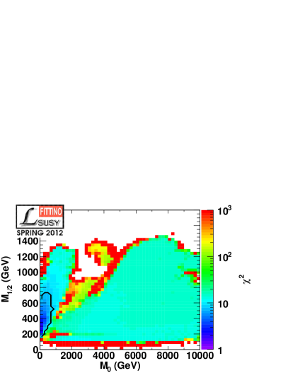
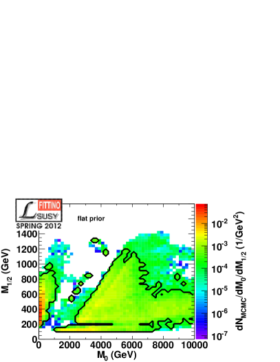
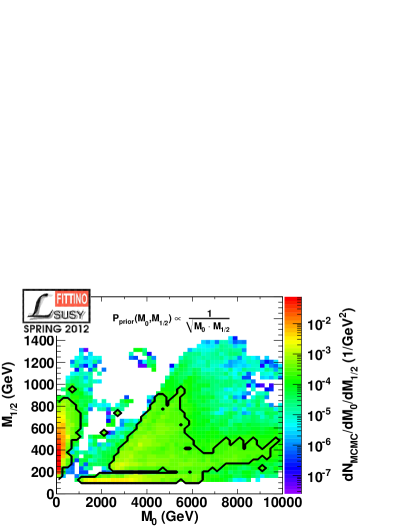
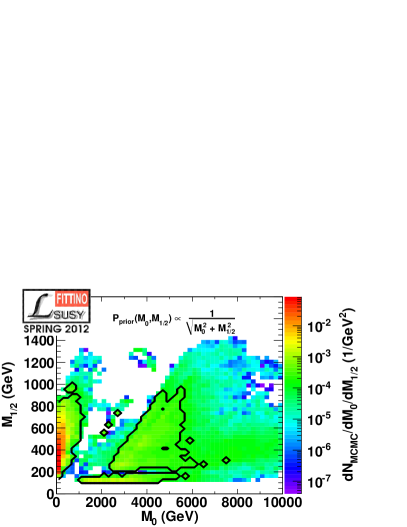
In Fig. 1, both interpretations are shown for an example fit in order to illustrate the differences. The fit is performed using the same setup as in Bechtle:2011dm . Only the observables listed in Tab. 2 are used, in contrast to Bechtle:2011dm . This example fit is only used for testing the statistical procedure, but not used for the results presented in Section 4. Figure 1 shows the 2-dimensional profile in the () plane. The small black contour on the left indicates the 2-dimensional region in the frequentist interpretation. Figure 1 instead shows the MCMC scan point-density in the same plane. The black contour indicates the 2-dimensional -CL region for the same fit using a flat prior. In the white area, no points have been reached by the MCMC chain. Only scans with constant proposal density functions are used, in contrast to the continuous optimisation used for the other fits as described in Section 2.1 in order to keep the MCMC point density proportional to the posterior pdf. Note that for the frequentist interpretation also points which were rejected by the MCMC algorithm have been taken into account. This explains why there are small scanned areas in the () plane which appear in the plot for the frequentist interpretation but not in the plot for the Bayesian interpretation. The results of the frequentist and Bayesian interpretation for the example fit are summarised in Tab. LABEL:tab:BayesVsFrequentist. Figures 1 and 1 show the Bayesian interpretation in the case of two different priors. Both priors have been chosen flat in and , while the dependence on and is chosen to be
Given the significant prior dependence of the results, we employ the frequentist interpretation for the results given in this paper. In addition, the frequentist interpretation allows us to increase the point density of the MCMC scans by also including rejected points and by optimising the proposal density function continuously during the fit. The appearance of the so-called focus point region (allowed points at rather low and very high ) in the Bayesian interpretation for the exactly same fit and the same MCMC chain as in the frequentist interpretation also helps to understand the significantly different allowed regions found in the literature in previous publications, see e.g. Fig. 1 in AbdusSalam:2011fc .
3 Experimental constraints
In this section, we describe the present and potential future experimental measurements and searches which we employ to constrain the supersymmetric parameter space. These can be grouped into three classes:
-
1.
Indirect constraints involving supersymmetric loop corrections;
-
2.
Constraints from astrophysical observations;
-
3.
Direct sparticle and Higgs boson search limits from high-energy colliders.
We discuss these groups of observables in turn below.
3.1 Indirect constraints
Supersymmetric particles may contribute to various low-energy observables through loop corrections. The various types of indirect constraints that can be utilized to explore the SUSY parameter space are
-
•
rare decays of B-mesons;
-
•
the anomalous magnetic moment of the muon;
-
•
electroweak precision observables.
The observables and their measured values as used in this paper are listed in Tab. 2. The different observables are briefly described in Sections 3.1.1 to 3.1.3. The Standard Model parameters that have been fixed are collected in Tab. 3. In one particular fit, the top quark mass is allowed to float.
| LEO:HFAG | ||
| LHCb-Moriond | ||
| LEO:HFAG | ||
| LEO:HFAG | ||
| Bennett:2006fi ; MuonAnom:Davier | ||
| GeV | MW-Moriond | |
| EW:Zres | ||
| Komatsu:2010fb | ||
| GeV | PDG2010 |
| MuonAnom:Davier | ||
| PDG2010 | ||
| PDG2010 | ||
| GeV | PDG2010 | |
| GeV | PDG2010 | |
| GeV | PDG2010 | |
| GeV | PDG2010 | |
| GeV | PDG2010 |
3.1.1 Rare decays of B mesons
Strong constraints on new physics models can be obtained from flavor observables, including, in particular, B-meson decays. The precise measurement of branching fractions of rare decays which are helicity suppressed or which are mediated only at the loop level by heavy particles, places important restrictions on the supersymmetric parameter space. Significant constraints come from oscillations, the branching fraction of and the inclusive branching fraction of . Recently there has been a substantial improvement in the limit on the branching ratio of the decay . The best limit is now LHCb-Moriond , which is used as a default in our fits. In addition, we study the impact of a potential observation of by LHCb LHCb:BsmumuProj at the SM rate of Buras:2010wr , i.e. assuming that no new physics is observed in this rare B-decay. Note that compared to our previous analyses Bechtle:2009ty ; Bechtle:2011dm ; Fittino:2011 , various observables from B- and K-meson decays have been discarded, as their contributions to the global fit have been found to be negligible.
3.1.2 The anomalous magnetic moment of the muon
Even though the anomalous magnetic moment of the electron is measured approximately two hundred times more precisely than that of the muon, , the sensitivity of to new physics is enhanced by a factor of , and thus represents a much more powerful constraint on the SUSY parameter space. While the measurement of Bennett:2006fi is undisputed, there is an ongoing debate about the accuracy of its Standard Model prediction MuonAnom:Davier . In particular, the non-perturbative contribution to from the hadronic vacuum polarization has to be extracted from experiment, via the data from annihilation to hadrons or from -lepton decays. For our base-line fit we have chosen the value of based on data, which has been argued to be theoretically cleaner than that based on decays. Note that in the CMSSM there is a strong correlation between and Dedes:2001fv .
3.1.3 Electroweak observables
In contrast to our previous analyses Bechtle:2009ty ; Bechtle:2011dm ; Fittino:2011 , the measurements of the Z-boson width and couplings, and the hadronic cross-section on the Z pole have been excluded from the fit. Indeed, despite their high precision and the absence of any ambiguity in the interpretation of the measurement, the contributions of these observables to the fit have been found to be negligible. Relevant constraints only come from the effective weak mixing angle and the W-boson mass. The values of the SM gauge couplings, and of the bottom, charm, and -lepton masses are fixed inputs to the fit, see Tab. 3.
3.2 Astrophysical constraints
Further constraints arise from astrophysical and cosmological observations such as the cold dark matter relic density as well as from direct and indirect dark matter searches. We use AstroFit AstroFit for the evaluation of the direct and indirect detection of dark matter observables. The relic density is provided by micrOMEGAs Belanger:2008sj . AstroFit provides an interface to DarkSUSY darksusy and adds an extensive database of relevant astrophysical data to the Fittino fit process. In particular, the particle spectrum and couplings of a given SUSY model are passed from Fittino using the SLHA standard Skands:2003cj ; Allanach:2008qq to AstroFit which uses various DarkSUSY applications to calculate the predictions for the requested observables . This result is then compared to actual experimental data and contributes to the as , where is the experimental measurement and the (combined statistical and systematic) error on it. For exclusion limits stated at a certain confidence level (e.g. from gamma-ray observations of dwarf spheroidal galaxies) or experimental results given in terms of confidence contours for claimed signals (as in the case of direct detection), AstroFit returns below the exclusion limit and inside the innermost confidence contour, respectively; outside this region, it interpolates between the values that correspond to the stated confidence levels and extrapolates quadratically beyond the largest explicitly given CLs (for limits, this is done by assuming that follows a Gaussian distribution around zero). On return, AstroFit passes the contribution from every included observable back to Fittino. In this paper, we use the dark matter relic density as well as the neutralino scattering and annihilation rates that are relevant for direct and indirect matter searches.
3.2.1 The cold dark matter relic density
Evidence for a considerable cold dark matter component in the composition of the Universe derives from a great number of observations that cover a large range of distance scales. In particular, the WMAP satellite has determined its cosmological abundance from observations of the cosmic microwave background to an impressive accuracy of Komatsu:2010fb . Weakly interacting massive particles (WIMPs), if neutral and stable on cosmological time scales, are very good candidates for the cosmological dark matter – the prime example being the lightest neutralino Jungman:1995df . Thermally produced in the early Universe, the WIMP relic density is set by the (co-)annihilation rate , see e.g. Refs. Gondolo:1990dk ; Edsjo:1997bg ; requiring that all dark matter is constituted by thermally produced neutralinos makes the relic density one of the most constraining observables for the CMSSM parameter space. In our fits, we calculate the relic density for comparison with both micrOMEGAs Belanger:2008sj and DarkSUSY darksusy (via the AstroFit interface). We add a 10% theory uncertainty in the calculation of the relic density due to missing higher order corrections in the anihilation cross sections Herrmann:2007ku ; Herrmann:2009wk ; Boudjema:2011ig .
3.2.2 Direct dark matter detection
Direct detection instruments look for elastic scattering events of WIMPs with nuclei of the according target material in underground laboratories. They detect signals via scintillation, phonons or ionization, depending on the experiment (see e.g. Cerdeno:2010jj for a review of direct dark matter detection). The spin-independent elastic scattering cross-section per nucleon, , conventionally adopted for a model-independent comparison between experimental results, is calculated with AstroFit, taking properly into account the potentially different scattering cross-sections on protons and neutrons. Theoretical uncertainties of approximately 20% from the so-called sigma-term Gasser:1990ce affect the calculation through changes to the form factor Cerdeno:2010jj . These uncertainties are estimated by varying the form factor within DarkSUSY and evaluating the resulting spread of the predicted value of for different points in the CMSSM parameter space along the expected exclusion. A resulting systematic uncertainty on of up to 50 % was found and added in quadrature to the experimental uncertainty obtained from the exclusion contour as described above.
Recently, controversial results have been reported from different direct detection experiments. While some of the collaborations, DAMA/LIBRA dama , CoGeNT cogent ; talk-collar and CRESST Angloher:2011uu , promulgate the detection of a signal, others, primarily XENON100 Aprile:2011hi , have shown upper limits nominally excluding the regions of signal detection. We adopt the current XENON limit as well as various projections including the XENON1T experiment as given in Ref. Baudis:2012bc . For an upper limit such as from XENON, the application of the aforementioned theoretical uncertainty on of 50 % translates into a maximally achievable contribution of 4 for the XENON limit. For the positive signals claimed by DAMA/LIBRA, CoGeNT and CRESST, no such limit applies directly. For those, we observe prohibitively high contributions and thus do not provide further fit results in Section 4.
3.2.3 Indirect dark matter detection
Indirect detection instruments – tracing products from dark matter annihilation such as photons, antiprotons, positrons, and neutrinos in the corresponding cosmic-ray fluxes – have been included via the gamma-ray channel (see e.g. Cirelli:2010xx for a review of indirect detection methods). Upper gamma-ray flux limits from dwarf spheroidal galaxies, preferred observation targets due to their high mass-to-light ratio and low background, from observations with Fermi-LAT fermi and H.E.S.S. hess have been included in the fit through AstroFit AstroFit .
We note that gamma-ray limits from dwarf spheroidals lead to the currently strongest model-independent bounds on the annihilation rate (at least for the range of dark matter masses that is relevant here). In this work, we therefore do not include available photon flux information from other sky regions, such as the galactic halo. The same holds true for other indirect detection channels, in particular antiprotons and positrons.
3.3 Direct search limits from high-energy colliders
Searches for supersymmetric particles have been performed at various high-energy colliders, with strong constraints on the MSSM particle spectrum, including supersymmetric Higgs bosons, specifically from LEP, the Tevatron, and the LHC. In the fits we include the limit on the lightest chargino mass from LEP, limits on the supersymmetric neutral and charged Higgs boson masses from LEP and the Tevatron, and, in particular, limits from recent LHC searches for supersymmetry in channels with jets and missing transverse energy.
3.3.1 The limit on the lightest chargino mass from LEP
The LEP collaborations have searched for charginos within the MSSM. The analyses assume gaugino mass unification at the GUT scale, , which leads to the relation at the electroweak scale. This holds for both the CMSSM and the NUHM1 considered here. The LEP collaborations searched for the dominant decay mode LEPSUSYWG . We have used the most conservative chargino mass limit of GeV, including a conservative estimate of the theoretical uncertainty of GeV. Because of gaugino mass unification, the limit on the chargino mass indirectly also excludes neutralinos with masses GeV in the constrained models considered here PDG2010 ; Dreiner:2009ic .
3.3.2 Limits on Higgs boson masses
The program HiggsBounds Bechtle:2011sb is used to implement the limits on the supersymmetric neutral and charged Higgs boson masses from LEP, the Tevatron and the LHC. HiggsBounds first determines the strongest search channel for the various Higgs signatures at every tested model point, based on the expected limit. For the SUSY models investigated here, the LEP limits on neutral Higgs bosons prevail in most of the relevant parameter space. The and values corresponding to these limits are tabulated in HiggsBounds for all signal strengths. Thus, even though the likelihood of the data for a given Higgs model is not directly available, the contribution from the Higgs searches can be calculated from the observed value for the most sensitive search channel and for any given Higgs mass and signal strength, with the valid assumption of a Gaussian distributions of . The relation
| (8) |
is used to determine the full contribution disregarding theoretical uncertainties of . The contribution of the Higgs limits to the total of the fit is then obtained from the distribution after folding with a Gaussian of width GeV to take into account the theory error Degrassi:2002fi ; Allanach:2004rh ; Heinemeyer:2004xw of the Higgs mass calculation. This procedure is implemented as an addition to HiggsBounds KarinaPrivateComm ; Ellis:2007fu .
In addition to the LEP results discussed above, the LHC collaborations have now presented an updated result on the combination of searches for the Standard Model Higgs boson ATLAS:2012ae ; Collaboration:2012tx with a combined allowed range at the 95 % CL limit of GeV, exceeding the LEP limit. No detailed translation of the values from the LHC-experiments into contributions is possible given the published values. Since the lightest Higgs boson in the CMSSM is SM-like, we can nevertheless study the effect of the new limit on the global fit in an approximate way by cutting on , taking into account also the theoretical uncertainty GeV. Furthermore, in a separate study we discuss the impact of a hypothetical SM-like Higgs boson signal at around GeV ATLAS:2012ae ; Collaboration:2012tx on global fits in the MSSM and the NUHM1.
3.3.3 SUSY searches at the LHC
At the LHC, the most stringent limits on supersymmetric models with R-parity conservation are obtained from searches in channels with jets and missing transverse energy, ATLAS-CMS-Moriond , where squarks and gluinos are produced in pairs and decay through and to purely hadronic final states with missing energy from the weakly interacting and stable lightest neutralino .
In order to properly include the SUSY exclusions from the LHC searches in the global SUSY fit, it is not sufficient to only consider the 95CL bounds published by the experimental collaborations for specific models and particular choices of parameters. Instead, it is mandatory to determine the corresponding contribution of the LHC observables, , for every point in parameter space. To that end we emulate the experimental SUSY search analyses by using state-of-the-art simulation tools and a public detector simulation to approximate the signal expectation for the specific model under consideration and any given set of model parameters. Details of the analysis are described below.
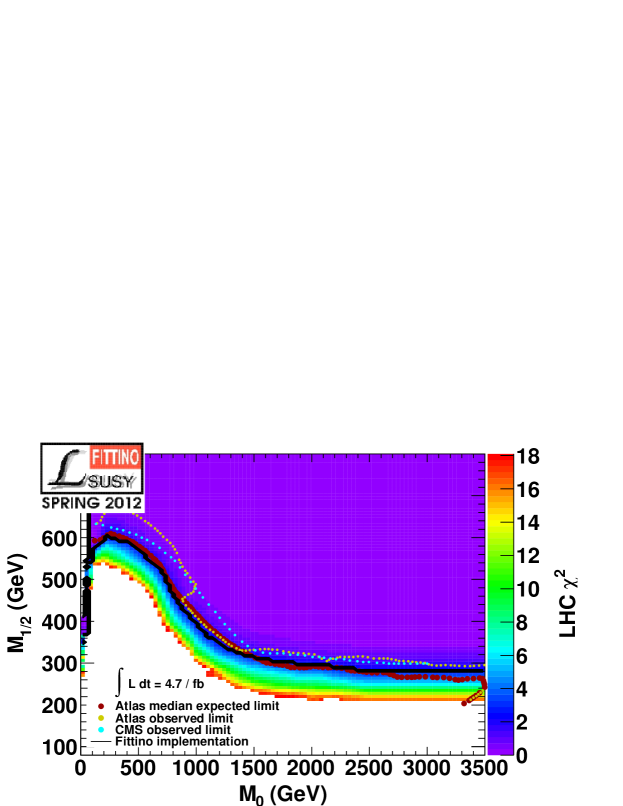
We determine the LHC SUSY exclusions from the search for squarks and gluinos using final states with 2, 3 or 4 jets, zero leptons, and missing transverse momentum, following a recent ATLAS analysis LHC:SUSYsearch . The signal cross-section is simulated on a grid in the plane, fixing , and . (We discuss the dependence of the signal on and below.) First, for each point of the grid, the SUSY mass spectrum is calculated with SPheno 3.1.0 SPheno . Events are then generated using Herwig 2.4.2 Bahr:2008pv and passed on to the fast detector simulation DELPHES.1.9 Ovyn:2009tx where reconstruction and detector smearing are performed. The efficiencies and fake rates of particle identification given by DELPHES are corrected using public measurements of detector resolutions by ATLAS RECSIM . Finally, the events have to pass the selection cuts specified in LHC:SUSYsearch .
The signal estimate is normalized to the NLO+NLL SUSY-QCD prediction for the inclusive squark and gluino cross-sections Beenakker:1996ch ; Beenakker:1997ut ; Kulesza:2008jb ; Kulesza:2009kq ; Beenakker:2009ha ; Beenakker:2010nq ; Beenakker:2011fu and the NLO prediction for the production of electroweak sparticles Beenakker:1999xh . While the theoretical uncertainty of the signal cross-section varies along the parameter space, we assign a constant 30 % error to the signal yield, which is a conservative estimate in the vicinity of the current LHC sparticle exclusions. The variation of the signal yield with the remaining CMSSM parameters and has been studied carefully. We found that it is always well within the systematic uncertainty, as exemplified in Fig. 2 for two points in the parameter space.
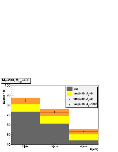
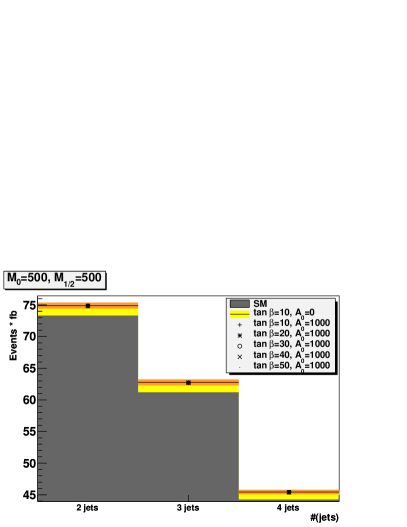
Our estimate of the SM background contribution is based on the ATLAS analysis LHC:SUSYsearch , which reports the results and statistical interpretation of the ATLAS fully hadronic inclusive SUSY searches using 165 pb-1 of integrated luminosity. A systematic uncertainty of 23% on the background has been estimated in LHC:SUSYsearch . Using the ATLAS background and background systematic uncertainty, together with a systematic uncertainty of on the signal cross-section, we can exactly reproduce the published ATLAS limits at and . The ATLAS analysis for , however, uses a profile likelihood based interpretation and six signal regions with tighter cuts. Because of the large amount of background control regions, this method cannot easily be implemented in an exact way within the fast Monte Carlo analysis used here. Most importantly, the background systematics are controlled within the profile likelihood technique. Therefore, we approximate the generic LHC results by reducing the systematic uncertainties used in the likelihood ratio analysis within realistic bounds and by slightly increasing the signal efficiency. Fig. 3 shows that this fast Monte Carlo technique is able to describe the LHC results within the 1 variation of the expected limit, both in scale as well as in shape. Thus, this method should provide a good description of the contribution at every point in SUSY parameter space.
The exclusion limit is calculated in the parameter space for each point with expected yields for signal and background and observed yield , calculating a test statistic , with being the likelihood ratio:
| (9) |
with the Poisson statistics , the number of expected and observed events, and , respectively, for the given point. The value of is a function of the SUSY parameters, whilst is fixed. The additional uncertainties are taken into account by a smearing of the Poisson distribution, and we consider a signal excluded with 95 CL if
| (10) |
with the probability density function of assuming the presence of a signal, and the actually observed value of . A given value can be approximately translated into a contribution using Ellis:2007fu :
| (11) |
To obtain the expected exclusion limits the Asimov data set was used.
4 Results
In this section, we present the results of our CMSSM and NUHM1 fits for various sets of input observables. We first summarize our general findings and then discuss the features of the different fits in more detail in Sections 4.1 to 4.5.
In Tables 4 and 5, we display selected results of the fits within the CMSSM and the NUHM1 for various sets of input observables. For all fits we require the lightest neutralino to be the LSP, consistent radiative electroweak symmetry breaking and the absence of tachyons.
| Fit | / | ||||
|---|---|---|---|---|---|
| LEO | 10.3/8 | ||||
| LHC | 13.1/9 | ||||
| LHC+XENON1T | 15.0/9 | ||||
| LHC+ GeV | 18.4/9 |
| Fit | / | |||||
|---|---|---|---|---|---|---|
| NUHM1+ | 15.3/8 |
In total, 7 different input parameter sets have been tested for the CMSSM. The fits based on the CoGeNT333The fit involving DAMA/LIBRA data has been omitted entirely since the CoGeNT regions lie closer to the accessible space in the CMSSM. cogent direct dark matter detection claim yield a prohibitively large minimal , implying that these potential DM observations cannot be accommodated within the CMSSM. We thus do not discuss them further. For all fits we require the lightest neutralino to be the LSP, consistent radiative electroweak symmetry breaking and the absence of tachyons. Note that a positive sign of is preferred to describe the anomalous magnetic moment of the muon, so we have fixed sgn in our fits.
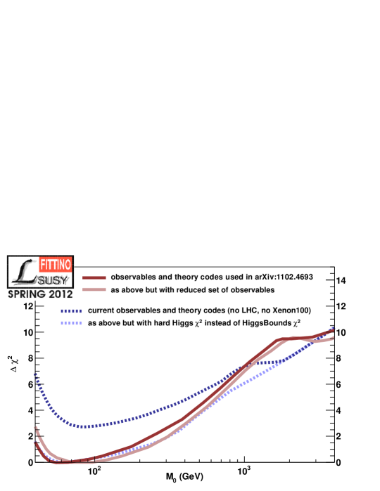
The fit labeled “LEO” (“low energy observables”) in Tab. 4 is performed excluding the direct search for SUSY at the LHC, but including all constraints from supersymmetric loop corrections (Section 3.1), astrophysical observations (3.2) and sparticle and Higgs boson search limits from LEP and the Tevatron (3.3.1 and 3.3.2). The best fit point and the 1-dimensional 1 parameter uncertainties are in excellent agreement with earlier studies Bechtle:2011dm , despite the fact that only a fraction of the observable set from Bechtle:2011dm is used here. As mentioned in Sections 3.1.1 and 3.1.3 various flavor and electroweak precision observables have been omitted from the fit, as they do not add significant information for constrained SUSY models. Instead they add a constant offset to the , which is nearly independent of the SUSY parameter point or model under study. The offset only depends on the SM parameters and the SM precision observables themselves. In Ref. Bechtle:2009ty it has been shown that the SM parameters decouple completely from the CMSSM parameters for the observables used here. Therefore, a reduced observable set results in a clearer message on the actual agreement of the SUSY prediction with the relevant data for a given model point. This is shown in Fig. 4. The red lines show the profile of the minimum of the fit as a function of , once with the full observable set from Bechtle:2011dm (dark red), and once with only the set of observables described in Section 3 (light red), but using the theory codes and observable vales from Bechtle:2011dm . No significant difference can be observed.
An interesting effect can be observed for the observable : While SUSY points with strong disagreement to the measurement exist, the majority of the allowed region exhibits a prediction of near its SM value, since the SUSY contribution tends to decrease the branching fraction, leading to stronger disagreement than in the SM. Thus, also contributes to a constant offset of the with respect to previous results with lower observed values of the branching fraction (e.g. Bechtle:2009ty ), while having no significant effect on the allowed region above the minimum.
In determining the number of degrees of freedom, , we include one-sided bounds as measurements, also if the minimum of the fit fulfills the bound. This is justified because the model exhibits parameter points violating the bounds. Removing the bound from the count as soon as the minimum or the regions directly around it satisfy it, would mean that the model is penalized for being consistent with the data on the ground of constraints from other observables. Therefore, all bounds with potential contribution to the are counted in .
Using the new observable set, and the new set of codes for the prediction of the observables as outlined in Sections 2 and 3, we obtain a of 10.3/8, hinting at a worse agreement than using the full observable set Bechtle:2011dm . However, as outlined in Section 2.2, no exact -value can be calculated due to computational limitations and the non-Gaussian nature of the fit. Clearly the overall fit quality of the CMSSM is reduced when using the reduced observable set of Tab. 2, and taking the improvements in the sensitivity of the measurements between the old and new observable set into account. Additional small effects stem from the update to newer versions of theory codes as outlined in Section 2.1.
Another significant difference between the fit results from Bechtle:2011dm and the results presented here is the more precise treatment of the LEP Higgs limits. In Bechtle:2011dm , HiggsBounds was used to calculate the exact position of the CL on for each model point. Then, the left half of a parabola corresponding to a theoretical uncertainty of GeV and with the minimum of at the exact CL point was used to calculate . Model points above the actual limit received a contribution of , while model points below received a contribution corresponding to the theoretical uncertainty.
For the results presented here, HiggsBounds is used to calculate the exact for every below and above the CL bound, folded with the theoretical uncertainty (see Section 3.3.2). Since for the best fit point of the LEO input set we obtain GeV, adding the actual contribution to the minimum makes a significant difference in the overall of the minimum. This can be seen from the blue lines of Fig. 4. The minimum in the dark blue curve is lifted significantly with respect to the fits without HiggsBounds (light blue). Since larger values of TeV yield GeV, does not contribute to the fit for large and the two lines are in perfect agreement for large . Thus, a thin stripe of the focus point region at large and very small is included in the allowed region, see Sec. 4.1. Its width in is mostly constrained by requiring GeV. The pull plot in Fig. 5 shows the contribution of the individual observables to the best fit point of the LEO fit.
The fit labeled “LHC” in Tab. 4 uses the same input as the LEO fit, plus the results from the LHC SUSY search described in Section 3.3.3. The effect of the LHC limit is a shift of the minimal and an increase of the number of degrees of freedom to . This clearly shows a further reduced agreement of the fit with the data, and the minimum is found at higher , and .
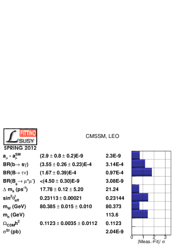
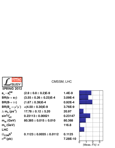
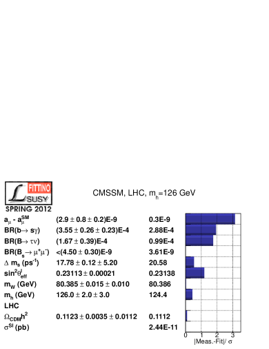
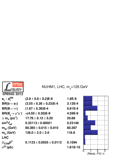
From the pull plot in Fig. 5 one can deduce that the LHC limit pushes the fit into a region where, in particular, is not described very well anymore. In comparison, the direct contribution of is small at the best fit point. The reason is that the contribution from the low energy observables is almost constant for large enough and . Thus, if the LHC pushes the fit above a certain threshold in the mass scale, the minimum can also move higher until is not dominant anymore. In addition, also prefers higher sparticle masses, balancing the push to lower mass scales from the precision observables. A further consequence of the LHC exclusions is that the preferred Higgs mass is shifted upwards to GeV.
The fit labeled “LHC+XENON1T” in Tab. 4 uses all the results from Tab. 2 and the direct LHC SUSY search, but the current XENON100 limit replaced by the projection for XENON 1T as outlined in Section 3.2.2, assuming no observation. The XENON 1T projection increases the minimal to 15.0. In order to achieve lower direct detection cross-sections, the fit is pushed to somewhat lower values of and excludes large positive values of , resulting in an dependence which is almost symmetric around . The detailed reasons are given in Section 4.4.
We have also considered the possibility that is measured at its SM value of at LHCb LHCb:BsmumuProj (instead of the otherwise employed limit of ). Since the minimum of the LHC fit predicts near its SM value, no significant change in fit probability or best fit point is observed, see the discussion in Section 4.2.
The new limits on the SM Higgs boson mass of GeV at CL ATLAS:2012ae ; Collaboration:2012tx from the ATLAS and CMS experiments are not included in the detailed calculation in HiggsBounds. Therefore, no detailed calculation of the contribution from that constraint is performed. However, applying a simple cut of GeV (including a theoretical uncertainty of GeV) on the LHC fit does not lead to a significant effect on the allowed parameter space, since for the largest part of the parameter space in the LHC fit is predicted in the allowed range due to the heavy sparticle mass scales.
Finally, we explore a possible Higgs observation at GeV, as outlined in Section 3.3.2. The corresponding fit is called “LHC+126” in Table 4. Apart from exchanging the HiggsBounds result for for the assumption of a direct measurement, the inputs to the fit are identical to the LHC fit. The high sparticle masses required to yield such a high Higgs mass push the best fit point into the focus point region at TeV. The shows that GeV is hardly compatible with a highly constrained SUSY model such as the CMSSM. This is also obvious from the pull contributions in Fig. 5. While a sufficiently high value of GeV can be reached for the best fit point, the necessary high sparticle mass scales push the fit into a region which is incompatible with and -physics observables at the 2 to 3 level.
By decoupling the Higgs sector from the squark and slepton sector in the NUHM1 model, this problem can be partly remedied. As shown in Tab. 5 and Fig. 5, a slightly better fit is possible for the NUHM1 () than for the CMSSM fit with GeV, albeit with reduced . Also, the added degree of freedom deepens the profile for and around the minimum, since the Higgs limit does not push the fit into an area with limited agreement between predictions and indirect observables. For a more detailed description of the NUHM1 fit, see Section 4.3.
In the following sections, the results for individual input observable sets are discussed in detail.
4.1 Fit without LHC exclusions
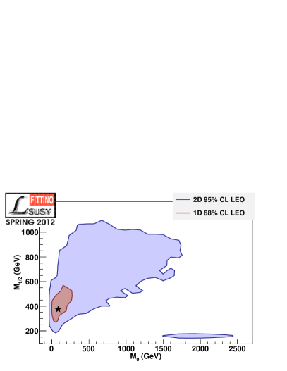
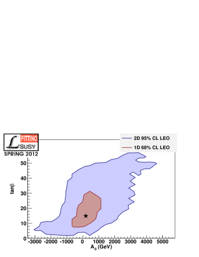
In Fig. 6 the resulting parameter regions are shown for the LEO fit. The best-fit point is marked by a star. All hidden dimensions are profiled. As in all further plots of the allowed parameter space, the allowed regions display the full (1-dimensional 1) range in red and the (2-dimensional 2) range in blue. The 1-dimensional 1 range is shown in order to allow reading off the single parameter uncertainties directly from the projection of the red areas onto the horizontal and vertical axes.
The resulting plot does not represent a parameter scan in the shown dimensions with fixed hidden dimensions, but the full uncertainty regions for the global fit of the four CMSSM parameters. As shown in Bechtle:2011dm , including the SM parameters in the fit does not change the result as long as the presently available observables are used. This may change in the future, e.g. once very precise measurements of or sparticle masses are available.
In contrast to the results from Bechtle:2011dm , and in contrast to the profile likelihood result from Fig. 1 which uses the observable set and prediction codes from Bechtle:2011dm , the focus point region at low and high is allowed within the 2-dimensional uncertainty range. This is explained by the cut through the profile already shown in Fig. 4. The focus point region is constrained to GeV by the presence of the cut on GeV described in Section 3.3.1. The minimal shape in Fig. 4 also explains why the allowed region is so much larger than what would be expected from the region. The fit exhibits a rather narrow minimum, where a good agreement with and can be achieved. For larger values of and , there is an almost constant disagreement with both measurements at the level. Hence, no further discrimination is achieved and the profile becomes almost flat, still within the range above the minimum.
4.2 Fits with LHC exclusions
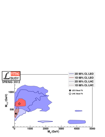
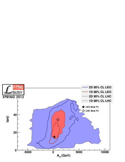
In this section, we discuss the allowed CMSSM parameter space for different inputs from the LHC. The inputs with the strongest impact are the inclusive direct searches for SUSY at the ATLAS experiment described in detail in Section 3.3.3 and the search for described in Section 3.1.1. The additional very strong constraint stemming from a possible measurement of the lightest Higgs boson mass is studied separately in Section 4.3. Fig. 7 shows the allowed parameter range of the LHC fit introduced in Table 4. The difference between the LHC and the LEO fit is significant. The position of the best-fit point is lifted outside of the directly accessible range of sparticle searches at low and GeV. The focus point region is excluded by the LHC SUSY search up to our maximum value of TeV of the LHC limit implementation. Also the LHC collaborations do not publish search results for larger values of , but it can be assumed that a dedicated interpretation at LHC would exclude large parts of the rest of the focus point region from the fit (i.e. the two islands above TeV in Fig. 7). Due to the diminishing relevance of large SUSY mass scales for the solution of the hierarchy problem and EWSB, this is not further pursued here.
It can be observed in Fig. 7 that the best fit point of is shifted upwards significantly due to the direct LHC SUSY search limits, which do not affect directly, as shown in detail in Section 3.3.3. This is the result of the correlation between on the one hand and on the other hand due to and . A decent agreement in those variables for larger implies higher scales of .
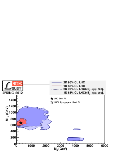
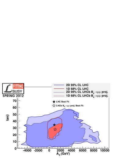
In Fig. 8 we use the LHC limits as outlined above and in addition study variations of the limit on . In Fig. 8 and 8, the results of the fit including a potential measurement at the SM value (assuming a small theoretical and experimental error of for the sake of studying the strongest possible impact) at LHCb LHCb:BsmumuProj and possibly ATLAS and CMS is shown. Since the best-fit point of the LHC fit predicts close to its SM value, this has only a marginal effect on the minimal of the fit and the allowed parameter space. Note that the situation would have been somewhat different for a potential observation of at CDF CDF:Bsmumu , which would have clearly disfavored the focus point region.
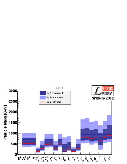
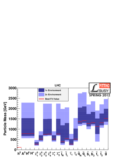
We show the predicted range of sparticle and Higgs boson masses for the LHC fit in Fig. 9 compared to the same prediction for the LEO fit in Fig. 9. As discussed above and in Fig. 4, the flat profile for large and predicts sparticle masses at TeV for both the LEO and LHC fits. The only particle with a very strong upper bound on its mass is the lightest Higgs boson. The prediction of changes from GeV for the LEO fit to GeV for the LHC fit. The 1-dimensional range quoted here is clearly incompatible with the potential signal at GeV. However the profile is flatter for higher , making it marginally possible to reconcile a heavier Higgs mass with the CMSSM, as outlined in Section 4.3. In addition, the lightest neutralino is bound from above at GeV, as a result of the combined constraints on and .
We note that also in the LHC fit there is still enough room for slepton and gaugino masses below GeV, which would be observable at an linear collider with TeV, despite the stringent search limits from the LHC. This is partly due to the fact that the LHC allowed region extends slightly below the 95 % CL exclusion. The increasing LHC contribution for smaller sparticle mass scales is partly canceled by the decreasing contribution from the LEO observables. The stronger effect however is the fact that even highly constrained models as the CMSSM still exhibit enough freedom in the parameter space to reconcile light gauginos and sleptons with heavy squarks and gluinos, as shown in Fig. 9. This feature would be even more pronounced in more general SUSY models, in which the colored and the non-colored sectors explicitly decouple.
4.3 Adding a potential Higgs boson mass measurement
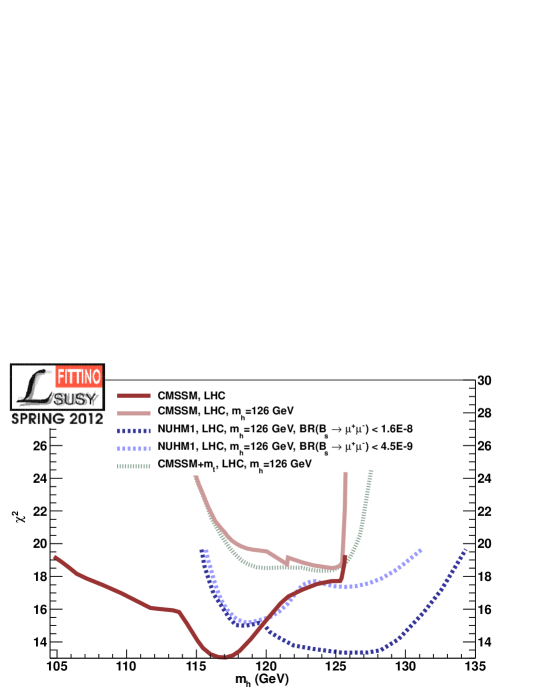
A very strong constraint on the CMSSM is expected from a direct measurement of the lightest Higgs boson mass . This is shown explicitly in Fig. 10, where we display the profile of for different fits: the LHC fit, the LHC+126 fit with fixed , the same with GeV floating, and the NUHM1 fit with the same observables. It can be seen that the CMSSM fits (red and green curves) can barely incorporate GeV. At this edge the rises dramatically excluding any higher Higgs boson mass values. This limit is just slightly increased by floating (green curve), but the overall of this fit is still at the same rather inconsistent level of 18/9 as for the fit with fixed , for which 18.4/9 is observed. It is obvious that the NUHM1 fit, which decouples the Higgs boson mass parameter squared from at the GUT scale, shows both a significantly better agreement of and the ability to accommodate higher values of .
In Ref. Dedes:2001fv a strong correlation between and was observed for fixed . It was shown that the correlated region for the current experimental values of and is inconsistent with a Higgs boson mass at GeV. Accordingly the pull plot Fig. 5 has a poor fit for . Performing a fit just for the three observables , , and GeV results in a penalty of 7 with respect to just fitting and . This explains the strong difference between the fits with and without GeV. To further exhibit the combined effect of the limit on and a potential Higgs boson observation, we show in Fig. 10 the profile of against for different options of the measurement of . While a measurement at the level of the SM of has no strong effect on the maximal achievable value of for the CMSSM fit, there is a significant difference for the NUHM1 fit, where large is disfavored for a low . Even the current LHCb limit severely impacts the fit quality with respect to a looser bound on , since the NUHM1 fit with GeV prefers . Of course this is not a general observation, since the -physics and the Higgs sector observables are not directly governed by the same parameters in the MSSM, while they are connected via GUT scale assumptions in the CMSSM and NUHM1. Therefore, also in this example, testing more general SUSY models than the CMSSM and the NUHM1 would be beneficial. However, the current limitations on the correct implementation of the LHC results, as outlined in Section 3.3.3, has to be overcome.
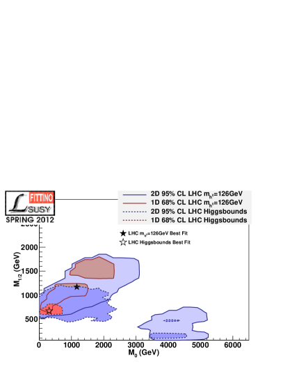
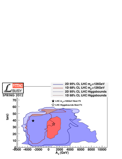
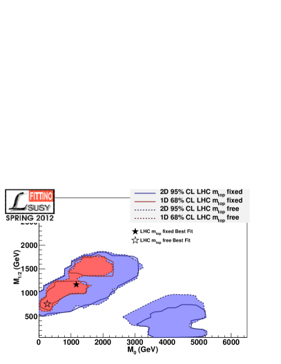
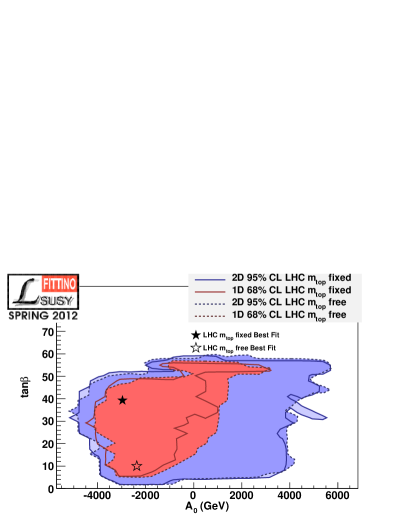
Figure 11 shows the allowed parameter range in the () and () planes for the CMSSM fits with fixed in Fig. 11 and 11 and with GeV floating in Fig. 11 and 11. The possible signal at GeV shifts the allowed region strongly into regions of higher and , as compared to the LHC fit. This is due to the larger squark masses necessary to lift so strongly above the tree level bound of . Also, large is clearly preferred, while again showing a flat profile in outside the region. As expected from the small effect which floating had on the fit in Fig. 10, there is no significant difference between the allowed parameter ranges for fixed and floating, albeit there is a significant jump in the best fit point due to the flatness of the profile. Since is expected to have the strongest direct effect on the prediction of all SM parameters, this confirms that with the current observable set the SM parameters can be fixed in the fit, since their uncertainties decouple completely from the SUSY parameter uncertainties.
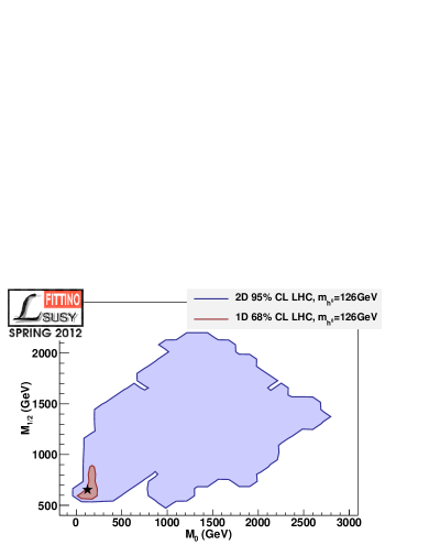
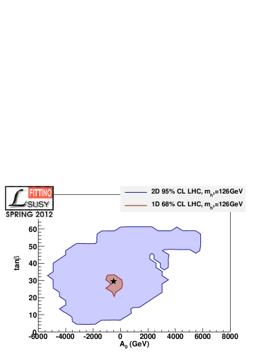
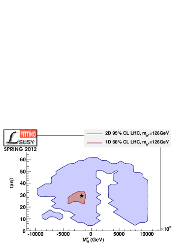
Figure 12 shows the allowed parameter space of the NUHM1 model. Negative values for can be considered because the relevant parameter combination for EWSB is , which we checked to be positive above the electroweak scale. Since this model reaches lower for the same observable set as the LHC+126 fit, its area of low is deep enough with respect to the surrounding flat profile (see Section 4.1 and 4.2) to exclude the focus point region from the 2-dimensional region. Other than that, no significant deviations from the CMSSM can be observed for and . However, the NUHM1 may also be sensitive to exclusions from the search for at the LHC. Unfortunately, these searches are not yet implemented in HiggsBounds in a model independent way, and hence not available for this fit.
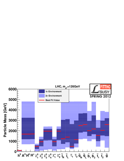
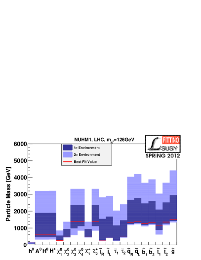
In Fig. 13, the predicted sparticle and Higgs boson mass range for the CMSSM with GeV is shown. As discussed above, the high value of can best be reached for high sparticle masses, shifting up the expected squark mass scale significantly with respect to Fig. 9. The NUHM1 fit is not pushed into the same area of a flat profile for heavy and as the CMSSM LHC+126 fit. Therefore, and because it can decouple the Higgs sector via the separate parameter , it prefers significantly lower sparticle and heavy Higgs boson mass scales than the CMSSM with the same observables.
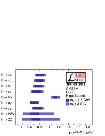
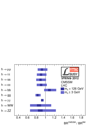
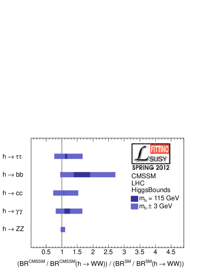
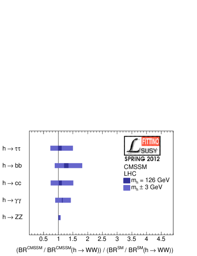
The observed fit results can be used to look at the range of allowed Higgs branching fractions in the CMSSM. These measurements are not used in the fit, and the range of predicted branching fraction values can be plotted within the allowed parameter range. Since the program HDECAY Djouadi:1997yw is not included in the fitting process, it is used after the determination of the allowed parameter range to predict the ratios of lightest Higgs branching fractions between the CMSSM and the SM. In order to do this, the parameters are scanned in a 4-dimensional grid around the best fit point within their 1-dimensional uncertainties. We assume that can be measured with an experimental precision of better than 2 GeV, once the branching fractions or ratios of branching fractions are measured with sufficient precision. The theoretical uncertainty of the prediction for must be taken into account for a prediction of . In Fig. 14 the allowed range of for various branching fractions is shown for the LHC fit at GeV. Fig. 14 shows the same for the CMSSM LHC+126 fit. In both cases one observes an enhancement of the final state. decreases due to different contributions to the enhanced terms which need to be resummed Carena:1999py ; Dedes:2002er . The main difference is in particular due to the gluino-sbottom and chargino-stop contributions in case of the final state. A significant sensitivity beyond the SM values can be observed in both cases, making potential measurements of the branching fractions Lafaye:2009vr very attractive to determine the model parameters further and to discover a deviation from the SM even for SUSY mass scales beyond the LHC reach at or TeV. In Fig. 14 and 14 it can be seen that even the (at the LHC) experimentally potentially accessible ratios of branching fractions still exhibit significant potential for discovering differences from the expected behavior of a SM Higgs boson. The effect of such measurements on the fit can be expected to be even stronger assuming the foreseen precision at an linear collider (see e.g. Djouadi:2007ik ).
4.4 Implications for dark matter searches
In the following we discuss the impact of the astrophysical input parameters on our fit results. Recall that adding the claimed signals in direct detection from the CoGeNT experiment cogent ; talk-collar to our fit leads to an unacceptably high contribution. We thus confirm earlier observations Baltz:2004aw revealing that the large scattering rates associated with these signals are incompatible with originating solely from neutralino DM in the CMSSM. The same holds for the DAMA/LIBRA dama signal.
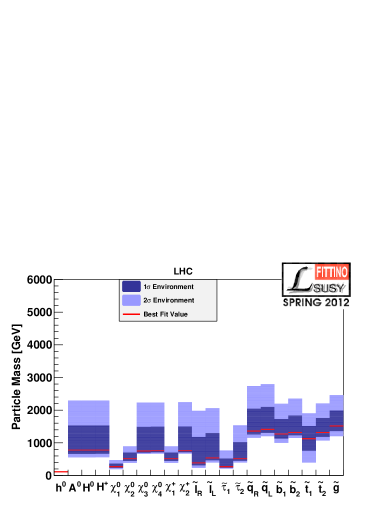
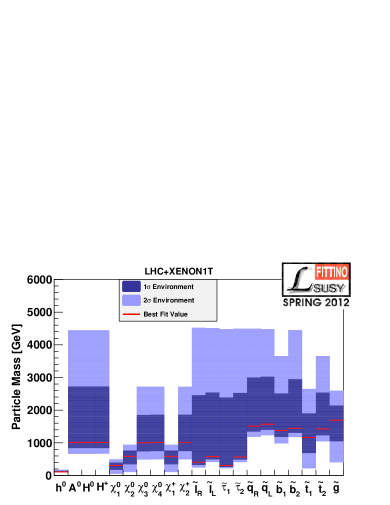
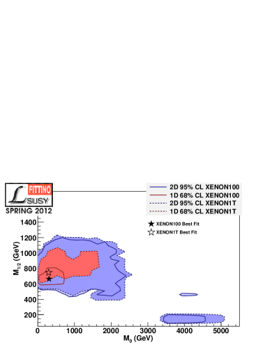
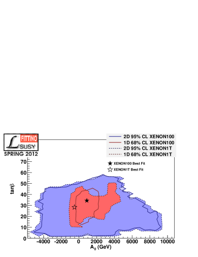
Upper limits from the Xenon100 Aprile:2011hi experiment presently do not constrain the CMSSM parameters beyond the LEO, LHC (5 fb-1) data and the relic density of CDM alone. Concerning future prospects Baudis:2012bc for direct detection, we find that stronger constraints on the spin-independent scattering cross-section per nucleon that would result from an increased runtime (as planned with XENON100Goal) and a non-observation do not have a large impact, either. Increasing the target mass (XENON1T) and a non-observation, on the other hand, would enlarge the allowed 68% CL region in both the () and the () plane (see Fig. 15) and move the best fit point to somewhat higher scales. At 95% CL, the contours comprise only slightly larger regions – with the largest change visible in the focus point region at TeV. The overall fit quality, however, becomes considerably worse in this case and the minimal increases from 13.1/9 to 15.0/9, as already stated in Table 4. In fact, Fig. 16 shows that implementing the projected XENON1T limits has the effect of considerably raising the best-fit mass of essentially all particles with respect to the current baseline expectation, in particular for the heavy Higgs bosons and squarks.
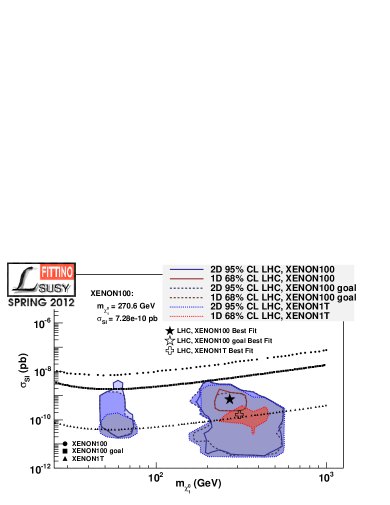
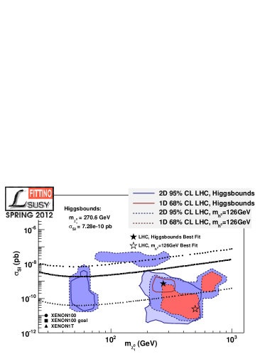
We also considered the combined impact of direct detection limits and a Higgs boson mass of GeV. In Fig. 17, we only use limits from HiggsBounds to constrain the Higgs boson mass: in an overlay plot, we show how constraints from direct detection experiments will hardly improve with increased runtime (XENON100Goal) but would do so with an increased target mass (XENON1T) – however at the cost of an increased , see the comment above. Note that our XENON1T allowed region extends into the regions nominally excluded by the experiment. The reason for this is that we adopted the rather conservative choice of assigning a theoretical uncertainty of to the calculation of the spin-independent scattering cross-section per nucleon , see Section 3.2.2. Restricting the Higgs boson mass to GeV instead, we see in Fig. 17 that the preferred neutralino mass moves from GeV to GeV; this trend to higher masses is of course expected because a large Higgs boson mass generally requires rather high values for the SUSY breaking scale (at least in the minimal SUSY version considered here). Concerning future prospects for direct detection, we can see that a large Higgs boson mass worsens the situation as it pushes the best-fit to lower values.
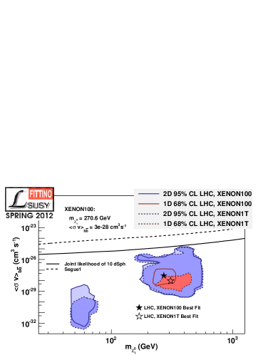
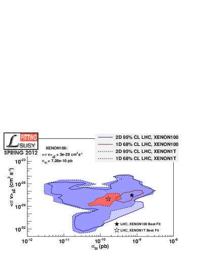
We find that our indirect detection upper limits from dwarf spheroidal galaxies, using gamma-ray observations by the Fermi satellite, are still too weak to give a noticeable -contribution for neutralino DM in the CMSSM. This is not a great surprise as the limits barely touch the annihilation cross-section of , which is naively expected for thermally produced DM. Concretely, we used the photon flux upper limits from Ref. Abdo:2010ex , for MeV, on neutralino pair annihilation into final states – which very often gives the dominant contribution to the total flux (mostly from photons with ). An improved treatment would also take into account the photons from other final states. However we caution that this is not straightforward to implement in those regions of the parameter space where the photon spectra are very model-dependent Bringmann:2007nk . Further improvement is possible by using updated limits from a combined (‘stacked’) analysis of all dwarf spheroidal galaxy data taken by Fermi Ackermann:2011wa . We thus expect that a more accurate treatment of the combined gamma-ray limits in AstroFit, which is planned for future fits, would actually impact the CMSSM parameter space (as also found in e.g. Ref. Scott:2009jn ). This expectation is reflected in Fig. 18, where we show vs. : While the limits that we have implemented indeed do not touch the regions, the improved limits from the joined dwarf spheroidal galaxy analysis Ackermann:2011wa do. Those limits were not available in AstroFit when the scans were set up. Let us also stress that we plot here only the annihilation cross-section into final states. Future prospects for indirect dark matter detection are thus actually much better than what is naively inferred from this figure – especially when explicitly taking into account gamma-ray spectral features in the analysis rather than only counting the number of photons Bringmann:2012vr .
In Fig. 18, we plot the neutralino annihilation cross-section against the spin-independent scattering cross-section, demonstrating that indirect and direct dark matter searches indeed probe the parameter space from an orthogonal direction Bergstrom:2010gh and are highly complementary even for very constrained scenarios like the CMSSM. In particular, improving current gamma-ray limits by about one order of magnitude (as might be rather straight-forward with future air Ĉerenkov telescopes Bergstrom:2010gh ) would allow to probe models that are completely out of reach even for XENON1T. Models in the upper right corner of Fig. 18, on the other hand, would in principle allow for a future simultaneous detection of dark matter with both direct and indirect methods which evidently would make any claim for a corresponding signal much more convincing. We checked that adding the Higgs-mass constraint GeV does not have a major impact on the 2 region in this plane. The 1 region, on the other, hand blows up considerably. The best fit point moves to pb and cm3s-1. This again just reflects the overall worse quality of the fit.
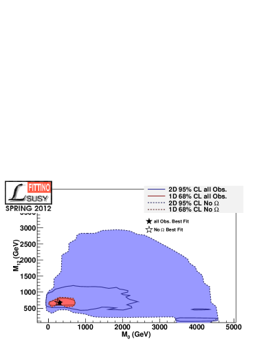
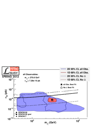
The relic density of cold dark matter remains a strong constraint on the fit. Indeed, it is well known that only relatively small regions in the full parameter space of the CMSSM can account for thermally produced neutralino dark matter with the correct relic density: (i) the bulk region at low values of and , which is now essentially excluded by collider data, (ii) the funnel region at intermediate values of and with so that annihilation via the pseudo-scalar Higgs boson becomes resonant, (iii) the focus point region at where the lightest neutralino has a sizable Higgsino component and (iv) the stau co-annihilation region at large but small with . Moreover, for there is the stop co-annihilation region at somewhat larger values of and correspondingly very large values of . The impact of the relic density constraint can best be demonstrated in the plane, as shown in Fig.˜19. Note that for fixed values of and the allowed regions would only appear as thin strips in this plane. While we find that the relic density calculated by DarkSUSY darksusy and micrOMEGAs Belanger:2008sj can differ up to a factor two for some parameter combinations, this does not have a significant impact on our best fit regions and 2D contour plots. The most striking difference appears in Fig.˜19 where the co-annihilation region does not extend all the way out to TeV but only to TeV when using DarkSUSY instead of micrOMEGAs. Figure 19 shows that the relic density together with the particle physics input favors neutralino masses in the range between 200 GeV and 500 GeV. At 95% CL an additional range between 50 and 70 GeV is allowed. This corresponds to a resonance in the focus point region, see below. However, the expected spin-independent scattering cross-section is hardly affected by the relic density constraint.
Note that the region with GeV that appears in several of the 2D plots discussed above does not show up in the mass distribution plots (Fig. 16) because it is not contained in the 1-dimensional environment. These neutralinos lie in the focus point region appearing in Fig. 19 at very low values of and TeV. They have a Higgsino fraction of roughly 1%. Their relic density is almost exclusively set through -channel annihilation via the light scalar Higgs .
Moving along the focus point ‘strip’ to larger masses, the Higgsino fraction increases and at TeV the neutralino becomes an essentially pure Higgsino that acquires the correct relic density for TeV. In our fit, however, models with such large neutralino masses do not appear because the sampling algorithm runs out of statistics at these very large values of TeV due to the excessive inter-parameter fine-tuning (discussed in Section 4.6) for such high 444 See, however, Ref. Baer:2005ky for a detailed discussion of the focus point region arguing that, even for very large values of , the actual fine-tuning is small if expressed in physical parameters.. For the same reason, we do not sample the tail of the co-annihilation strip which in principle admits TeV-scale neutralinos co-annihilating with almost degenerate staus. We mention that the very small region at TeV and slightly higher values of also belongs to the focus point region. Albeit in this case it contains models where the lightest neutralino has a sizable Higgsino fraction of and a mass around 200 GeV. The relic density is thus mostly set through (non-resonant) annihilation into gauge bosons, which is helped by the presence of relatively light charginos and neutralinos, though not light enough that co-annihilations would be important.
4.5 Fine-tuning
A major motivation for supersymmetry at or near the electroweak scale is to solve the hierarchy problem Gildener:1976ai ; Veltman:1980mj . This is a fine-tuning problem in the Higgs sector of the theory, where the low-energy observable Higgs boson mass depends sensitively on the input parameters at a postulated new scale of physics, such as the unification scale , or the Planck scale. This fine-tuning is removed and the hierarchy problem solved for unbroken supersymmetry. A solution is retained after supersymmetry breaking, if the supersymmetry masses are not too heavy. How heavy depends on how much fine-tuning is perceived to be acceptable. This is the origin of the expectation, that the supersymmetric masses should be , or even less.
Beyond the Higgs boson mass, also other low-energy parameters can be fine-tuned, such as the electroweak breaking scale, represented by the boson mass, . The fine-tuning can be quantified by various measures. A popular one was introduced in Barbieri:1987fn . It is based on the logarithmic derivatives of any given observables with respect to the parameters considered. For considered as a function of variables the relevant numbers are
| (12) |
The overall fine-tuning at a given parameter point is then given by
| (13) |
It has since been widely used to quantify the fine-tuning in the (C)MSSM both before Chankowski:1997zh ; Barbieri:1998uv ; Chankowski:1998xv ; Batra:2003nj ; Giudice:2006sn ; Cassel:2009ps and more recently also including LHC data Cassel:2011tg ; Strumia:2011dy ; Ross:2011xv .
For the CMSSM, SOFTSUSY Allanach:2001kg can be configured to calculate all of the derivatives in Eq. (12). The set of parameters consists of , , , , , and .555SOFTSUSY also allows the computation of the derivatives with respect to the non-CMSSM parameters , the soft breaking gluino mass, and , the top Yukawa coupling. Points with larger values for are more fine-tuned and are in general regarded as less natural. A fit has been performed to assess the fine-tuning, using the same observables and LHC limit as for the LHC fit before, but with SoftSUSY as spectrum calculator instead of SPheno.
As we have seen, the LHC exclusion leads to an overall decrease of the fit quality. Despite having a more constrained system, this worse fit can lead to more points in the 2 allowed range around the best-fit point. In particular, for a fixed value in the - plane a larger range of and values can be allowed. In Fig. 20 we plot the lowest values of in the - plane, where the parameters and have been profiled.
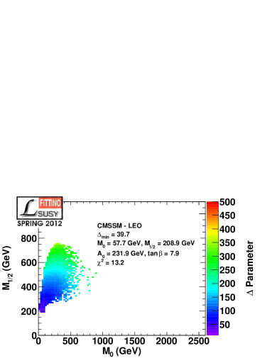
In Fig. 20, is shown for the pre-LHC fit. The lowest amounts of fine-tuning () are observed for low values of and , while in particular for high values of the -parameter reaches larger values, over 300.666We also considered the fine-tuning as a function of and for the best-fitting values of and in each bin. The results are indistinguishable from Fig. 20.
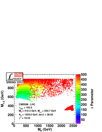
Fig. 20 shows the fine-tuning taking into account the LHC exclusion with a dataset of . This fit introduces points with a significantly larger fine-tuning () compared to the pre-LHC fit and the point of lowest fine-tuning (), is significantly more fine-tuned than in the pre-LHC fit. This is because the fit pushes one to higher values of . Again overall in the LHC fit, low values of and allow for a lower fine-tuning, while for larger values for both parameters, in particular in the focus point region, a higher fine-tuning is observed (see also discussion in Section 4.4).
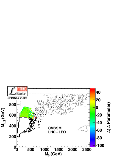
Fig. 20 shows the difference, , between the two fits in the region that is included in the -contours of both the pre-LHC as well as the LHC fit. The solid/dashed lines indicate the part of the parameter space which is not excluded at the -CL in the pre-LHC/LHC fit, but which is excluded at the -CL in the LHC/pre-LHC fit. In the plane, only a few points with a significant change in the fine-tuning show up, while for the majority of points which are not excluded in both fits, the fine-tuning is comparable.
We find slightly larger minimal values of compared to other studies, for instance Cassel:2011tg . However, the values we find are not dramatically larger and our fits are constrained by a larger set of observables, such that deviations are expected. While we find that with earlier LHC limits (), using the criteria of Cassel:2011tg , points with an acceptable amount of fine-tuning () remain in reasonable agreement with all precision measurements, the minimal value of is pushed above this threshold by the up to date LHC results.
4.6 Correlation of fundamental parameters
The fine tuning measure described in the previous section has many merits from a theoretical point of view. However, from an experimental point of view, there is one major shortcoming: The absolute change of an arbitrarily selected observable such as is experimentally of limited interest. The experimentally more meaningful quantity is the change of the observable relative to its uncertainty. Furthermore, experimentally we are interested in all observables chosen to calculate the , not only in one particular quantity of special theoretical interest.
Therefore, we propose a different view on looking at the naturalness of a model in the light of all observables and all uncertainties, inspired by the fine tuning. There, if one prediction for an observable depends strongly on varying one parameter, the agreement of all measurements with the predictions must be restored by varying other parameters in a correlated way. Therefore, we examine the correlation of the fundamental parameters in the fit as an additional information about how highly the parameters have to be tuned with respect to each other, measured in the form of the quantity defined below, in order to fulfill the same level of agreement with all data in the fit. Thus, all observables in the fit contribute with their current experimental precision to .
A priori, the fundamental parameters of the tested models are independent. If however, starting from a point in parameter space with a quality of fit , if one parameter is varied, the experimental bounds may force a correlated change in one of the other parameters, in order to maintain an equally good fit. A first order measure for the dependence is Pearson’s product-moment correlation coefficient. For each pair of parameters, , it is defined by
| (14) |
is the average value for the parameter and the standard deviation of the Parameter . Therefore .
The set of values of the parameters used for the computation of the average and standard deviation at a fixed point P in the parameter space is defined by the value of at this point, . We consider all points in the MCMC scan with a quality of fit in the range , where . These are very thin slices. All points included twice or more often in the MCMC scan are taken into account only once. If less than 6 points exist within the boundary the tested point is assigned no value and excluded from the further analysis.
For each point in the -CL region, we now compute the quantity
| (15) |
considering all 6 combinations of . For a fixed value of and , and with , profiled, we then compute the minimum of , , over the -CL region. Large values of mean the fit is highly correlated.
A model highly constrained by the observables with their given precision will naturally yield near the point with the exact minimum. Depending on the model, observables and precision, it may however show high (e.g. near 1) or low values of over the full allowed range, depending on how much the parameters need to be fine-tuned with respect to each other in order to achieve a given agreement between the model predictions and all data, taking the experimental and theoretical precision fully into account.
can describe features of the analyzed parameter space at very different scales. For low values of its value is dominantly built from the small scale structure of the parameter space. For larger values of , all parameters vary over a larger range and thus the included parameter space grows significantly and correlations on a more global scale are reflected.
In order to have a baseline comparison, we have first implemented this procedure without the experimental constraints considered throughout this paper. Instead we have explored the correlation where only a minimum set of requirements has been used to constrain the parameter space: we require (a) the lightest neutralino to be the LSP, (b) consistent radiative electroweak symmetry breaking and (c) the absence of tachyons. In order to have a meaningful comparison, the correlation between two parameters is not calculated over an infinite parameter range, but instead in a rectangular subset of the parameter space, the boundaries of which are defined by the maximum and minimum values of each of the four parameters as found in the -CL region of the LHC fit of the same model. After performing this procedure we find the maximum correlation between parameters with these minimal constraints is found to be smaller than . This is what the following results should be compared against.
The results of this study including the pre-LHC and LHC constraints are summarized in Fig. 21. In Fig. 21 we show in the - plane, when including only the pre-LHC constraints. and are profiled. We see that due to the now restricted parameter space the correlations are all above 0.75, and well above the 0.2 considered above. Moreover the correlation increases when increasing and in particular when increasing
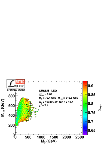
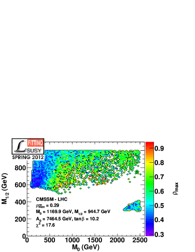
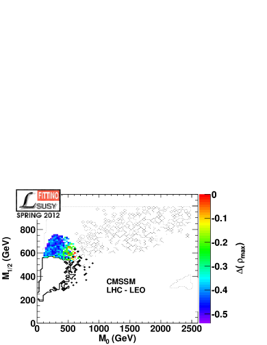
In Fig. 21 the LHC limits are now also taken into account. The colored region is significantly extended because the quality of the fit has gone down and the region is larger. At the same time, because and can extend over wider ranges, the correlation is markedly decreased compared to Fig. 21. It is however still everywhere above the baseline value of 0.2.
In Fig. 22, we consider slightly modified scenarios, with one additional fit parameter. In all cases we have fixed the lightest Higgs mass to GeV. In Fig. 22 [Fig. 22] we show the minimal correlation for a fixed (free) top mass, . Due to the fixed Higgs mass the quality of the fit degrades significantly. The 2 region is thus now extends to very high values of . For the free top mass the correlations are slightly higher than for the fixed case. In Fig. 22 we show the correlations in the case of the previously described model NUHM1. The minimum value of the correlation for this fit is 0.45. In all cases shown in Fig. 22, and , as well as and where applicable, are profiled.
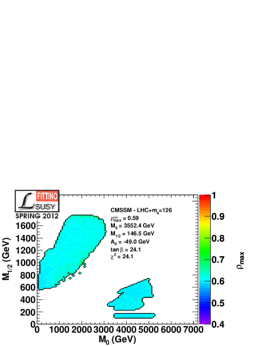
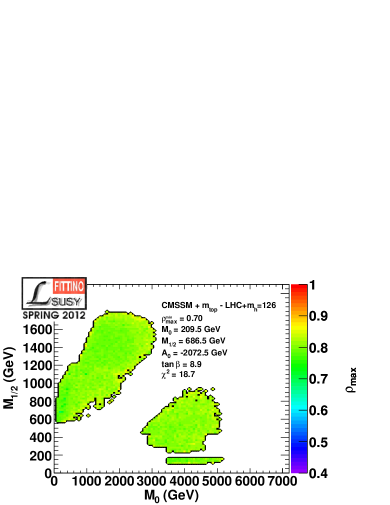
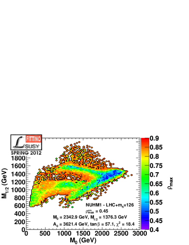
As discussed above, may vary significantly for similar values of and , if additional points with worse agreement between model predictions and measurements are reintroduced by adding another observable. This was so far taken into account by letting vary over the full accessible range, and then computing . It is also interesting to simply consider the best-fit value of for fixed values of . For the fits of the CMSSM model with GeV, this is shown in Fig. 23. Figs. 23/23 show in the - plane at the point with the lowest per bin for the =fixed/ = free fit. Figure 23 shows the difference between the two fits. A negative(positive) entry indicates that with =free(=fixed) a lower correlation between the parameters is found. In particular close to the minimum, = free allows for a lower correlation, while in other regions the maximum correlation between the varied parameters increases if the top mass is free. White areas indicate that at the corresponding point with the lowest there were less than 6 points within such that no meaningful correlation could be calculated.
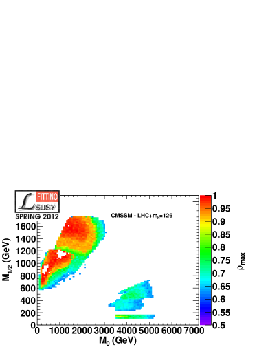
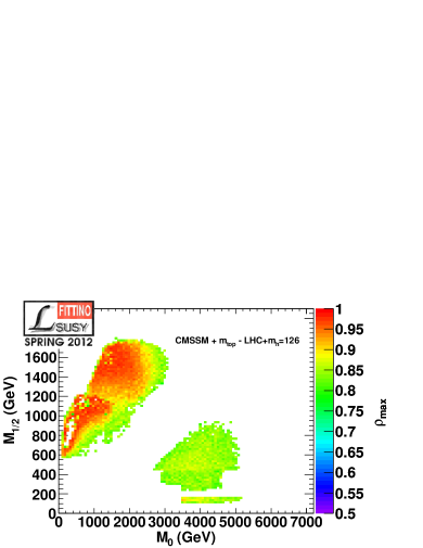
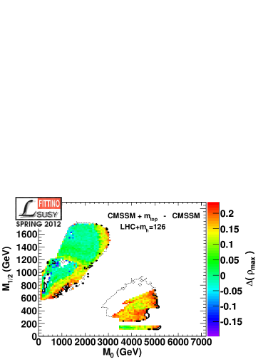
4.7 Including as a nuisance parameter
When fitting constrained models such as the CMSSM, the SUSY parameters are fitted at the GUT scale. The predictions for the observables are calculated from the MSSM Lagrangian calculated at a scale of TeV where we fixed the scale according to the SPA conventions AguilarSaavedra:2005pw . Theoretical uncertainties on the predictions are included in the calculation of the , as noted in Section 3. However, this does not included the parametric uncertainties arising from the fact that the masses are calculated using two-loop RGEs and one-loop (two-loop) threshold corrections for the sparticle (Higgs) masses. It is generally assumed in previous work in the literature (see e.g. Bechtle:2011dm ), that these uncertainties are negligible or at least sub-dominant for the observables described in Section 3.
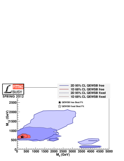
However, there is a straight-forward possibility to include these previously neglected uncertainties: The scale , where the spectrum is calculated, can be included as a nuisance parameter into the fit. It is allowed to float within . Then, the parameter uncertainties on the physical parameters of the model can be obtained by profiling over the hidden dimensions including . As shown in Fig. 24 for a fit including LHC exclusion, HiggsBounds limits and the full AstroFit limits, this has a sizable effect on the upper limit of the available parameter space, which is dominantly determined by and . The reason for this large increase is the flatness of the distribution which implies that already a small change can lead to the observed changes for the allowed regions. However, the best regions hardly changes. This result suggests that in future fits, the RGE uncertainty should be included as well.
We note for completeness that for very large values of and/or one obtains 1 TeV . However, in these regions the theoretical uncertainties for the mass calculations in codes likes SPheno or SoftSUSY is most likely larger than the scale variations suggests because here one should use a multi-scale approach as discussed in Baer:2005pv ; Box:2007ss ; Box:2008xu in contrast to the single scale approach of the current implementations Allanach:2001kg ; SPheno .
5 Conclusions
We have presented a global fit of the constrained MSSM and a non-universal Higgs mass model (NUHM1) to low-energy precision measurements, dark matter observables and, in particular, current LHC exclusion limits from direct SUSY searches in the zero-lepton plus jets and missing transverse energy channel. A restricted model with universal soft SUSY breaking parameters at the unification scale like the CMSSM does not provide a good description of all observables. The best fit predicts typical sparticle masses in the TeV-range, albeit with large errors. We find that the description of the low-energy observables, in particular, and the non-observation of SUSY at the LHC become increasingly incompatible within the CMSSM. Note that the LHC exclusion in the zero-lepton, jets plus channel mainly constrain the squark and gluino masses, while and other low-energy observables are sensitive to the color-neutral sparticles. Supersymmetric models with common scalar and gaugino masses like the CMSSM connect these two sectors and thus lead to an increasing tension between and the LHC search results, which would not necessarily be present in more general SUSY scenarios.
In general, there is an intricate interplay between the different contributions to the global fit, and an accurate estimate of the LHC exclusions also in parameter regions away from the published 95% CL contours is mandatory. We have thus employed an elaborate simulation of recent LHC search analyses based on state-of-the-art Monte-Carlo tools and a public detector simulation. We note that it appears challenging to provide a fast and accurate implementation of LHC results in a global fit for more general SUSY models with a larger number of parameters.
A very strong constraint on SUSY can be expected from a measurement of the light Higgs boson mass. Within the global CMSSM fit the light Higgs scalar is Standard-Model-like, with a preferred mass around GeV. We have studied the impact of a potential Higgs observation on the global fit and find that a light Higgs boson with mass GeV is hardly compatible with the other data within the CMSSM. The large sparticle mass scales needed to accommodate Higgs bosons with GeV drive the fit into a region which is incompatible with and -physics observables. This tension is reduced in models like the NUHM1 where the Higgs sector is decoupled from the squark and slepton sector. Still, even in the NUHM1, the interplay of and the lightest Higgs boson mass provides strong constraints. We have argued that important further constraints on SUSY models can be expected from improved limits on and, in particular, a measurement of the Higgs branching fractions or ratios of branching fractions. For the NUHM1, the search for pseudoscalar Higgs bosons in the channel will be another interesting input.
We have discussed in detail the implications of the CMSSM fit for direct and indirect dark matter searches. While direct dark matter detection claims from CoGeNT or DAMA/LIBRA cannot be accommodated within the CMSSM, the current upper direct detection limits provided by XENON do not restrict the CMSSM parameter space beyond the constraints from low-energy observables, LHC limits and the dark matter relic density. Projections of the direct dark matter detection limits based on a non-observation by XENON1T, on the other hand, would provide a further important probe of the available SUSY parameter space. The current indirect detection upper limits as implemented in AstroFit are still too weak to have an impact on the CMSSM fit. However, a more comprehensive future treatment of indirect detection limits may have the potential to probe the SUSY parameter space in regions which are complementary to direct detection constraints.
In addition, we have studied the fine-tuning within the SUSY models in two different ways. For the fine-tuning parameter , measuring the relative dependence of on all parameters, we find a strong increase between the fit without and with LHC direct search limits. For the CMSSM, a minimal value of is found for the LHC fit, which is generally regarded as unattractive. In addition, we introduce a new concept in the form of the relative precision at which the parameters need to be fine-tuned with respect to each other, in order to achieve the same overall agreement with all relevant observables relative to their uncertainties. Here, we find that within the uncertainty range the maximal correlations amongst parameters are still in the range of , hinting at an acceptable level of correlations. However, the correlation naturally increases strongly at the very minimum of the fit.
To further explore the implications of the LHC searches for supersymmetry it is mandatory to include a larger set of LHC signatures, including those which directly probe the non-colored sparticles, and to consider global fits of less restricted SUSY models beyond the CMSSM. The challenge for such future global analyses will be to provide a fast and accurate implementation of the LHC results, if possible for an accurate combination of different search channels, for more general SUSY models.
Acknowledgments
We thank Kevin Kröninger and Ben O’Leary for valuable discussions, and Wolfgang Ehrenfeld for invaluable computing support. We also thank the Helmholtz Alliance and DESY for providing Computing Infrastructure at the National Analysis Facility. This work has been supported in part by the Helmholtz Alliance “Physics at the Terascale”, the DFG SFB/TR9 “Computational Particle Physics”, the DFG SFB 676 “Particles, Strings and the Early Universe”, the European Community’s Marie-Curie Research Training Network under contract MRTN-CT-2006-035505 “Tools and Precision Calculations for Physics Discoveries at Colliders”, the DFG Emmy-Noether grant BR 3954/1-1, the DFG Emmy-Noether grant HE 5560/1-1 and the Helmholtz Young Investigator Grant VH-NG-303. MK thanks the CERN TH unit for hospitality. HD thanks SCIPP at UC Santa Cruz for hospitality during this work.
References
- (1) J. Wess and B. Zumino, Nucl. Phys. B 70 (1974) 39.
- (2) P. Langacker and M.-X. Luo, Phys. Rev. D 44 (1991) 817; U. Amaldi, W. de Boer and H. Furstenau, Phys. Lett. B 260 (1991) 447; J. R. Ellis, S. Kelley and D. V. Nanopoulos, Phys. Lett. B 260 (1991) 131.
- (3) E. Komatsu et al. [WMAP Collaboration], Astrophys. J. Suppl. 192 (2011) 18 [arXiv:1001.4538 [astro-ph.CO]].
- (4) H. Goldberg, Phys. Rev. Lett. 50 (1983) 1419 [Erratum-ibid. 103 (2009) 099905].
- (5) G. W. Bennett et al. [Muon G-2 Collaboration], Phys. Rev. D 73 (2006) 072003 [hep-ex/0602035].
- (6) Davier et al., CERN-OPEN-2010-021, LAL 10-155 Eur.Phys.J.C71:1515,2011
- (7) see Nakamura:2010zzi for a summary of limits on SUSY particles from LEP, SLC and the Tevatron.
- (8) G. Aad et al. [Atlas Collaboration], Phys. Rev. Lett. 106 (2011) 131802 [arXiv:1102.2357 [hep-ex]].
- (9) G. Aad et al. [Atlas Collaboration], Phys. Lett. B 701 (2011) 186 [arXiv:1102.5290 [hep-ex]].
- (10) G. Aad et al. [ATLAS Collaboration], Phys. Lett. B 701 (2011) 1 [arXiv:1103.1984 [hep-ex]].
- (11) G. Aad et al. [ATLAS Collaboration], Phys. Lett. B 701 (2011) 398 [arXiv:1103.4344 [hep-ex]].
- (12) G. Aad et al. [ATLAS Collaboration], Phys. Rev. Lett. 106 (2011) 251801 [arXiv:1103.5559 [hep-ex]].
- (13) G. Aad et al. [ATLAS Collaboration], Eur. Phys. J. C 71 (2011) 1647 [arXiv:1103.6208 [hep-ex]].
- (14) G. Aad et al. [ATLAS Collaboration], Eur. Phys. J. C 71 (2011) 1682 [arXiv:1103.6214 [hep-ex]].
- (15) G. Aad et al. [ATLAS Collaboration], Phys. Lett. B 703 (2011) 428 [arXiv:1106.4495 [hep-ex]].
- (16) G. Aad et al. [ATLAS Collaboration], Eur. Phys. J. C 71 (2011) 1744 [arXiv:1107.0561 [hep-ex]].
- (17) G. Aad et al. [ATLAS Collaboration], Phys. Lett. B 707 (2012) 478 [arXiv:1109.2242 [hep-ex]].
- (18) G. Aad [ATLAS Collaboration], Eur. Phys. J. C 71 (2011) 1809 [arXiv:1109.3089 [hep-ex]].
- (19) G. Aad et al. [ATLAS Collaboration], arXiv:1109.6572 [hep-ex].
- (20) G. Aad et al. [ATLAS Collaboration], Phys. Rev. D 85 (2012) 012006 [arXiv:1109.6606 [hep-ex]].
- (21) G. Aad et al. [Atlas Collaboration], JHEP 1111 (2011) 099 [arXiv:1110.2299 [hep-ex]].
- (22) G. Aad et al. [ATLAS Collaboration], Eur. Phys. J. C 71 (2011) 1828 [arXiv:1110.2693 [hep-ex]].
- (23) G. Aad et al. [ATLAS Collaboration], Phys. Lett. B 709 (2012) 137 [arXiv:1110.6189 [hep-ex]].
- (24) G. Aad et al. [ATLAS Collaboration], arXiv:1111.4116 [hep-ex].
- (25) [ATLAS Collaboration], arXiv:1112.3832 [hep-ex].
- (26) G. Aad et al. [ATLAS Collaboration], arXiv:1201.5595 [hep-ex].
- (27) [ATLAS Collaboration], arXiv:1202.4847 [hep-ex].
- (28) V. Khachatryan et al. [CMS Collaboration], Phys. Lett. B 698 (2011) 196 [arXiv:1101.1628 [hep-ex]].
- (29) S. Chatrchyan et al. [CMS Collaboration], Phys. Rev. Lett. 106 (2011) 211802 [arXiv:1103.0953 [hep-ex]].
- (30) S. Chatrchyan et al. [CMS Collaboration], JHEP 1106 (2011) 026 [arXiv:1103.1348 [hep-ex]].
- (31) S. Chatrchyan et al. [CMS Collaboration], JHEP 1106 (2011) 077 [arXiv:1104.3168 [hep-ex]].
- (32) S. Chatrchyan et al. [CMS Collaboration], JHEP 1106 (2011) 093 [arXiv:1105.3152 [hep-ex]].
- (33) S. Chatrchyan et al. [CMS Collaboration], Phys. Lett. B 704 (2011) 411 [arXiv:1106.0933 [hep-ex]].
- (34) S. Chatrchyan et al. [CMS Collaboration], JHEP 1107 (2011) 113 [arXiv:1106.3272 [hep-ex]].
- (35) S. Chatrchyan et al. [CMS Collaboration], Phys. Rev. D 85 (2012) 012004 [arXiv:1107.1279 [hep-ex]].
- (36) S. Chatrchyan et al. [CMS Collaboration], JHEP 1108 (2011) 156 [arXiv:1107.1870 [hep-ex]].
- (37) S. Chatrchyan et al. [CMS Collaboration], Phys. Rev. Lett. 107 (2011) 221804 [arXiv:1109.2352 [hep-ex]].
- (38) S. Chatrchyan et al. [CMS Collaboration], JHEP 1108 (2011) 155 [arXiv:1106.4503 [hep-ex]].
- (39) E. Aprile et al. [XENON100 Collaboration], Phys. Rev. Lett. 107 (2011) 131302 [arXiv:1104.2549 [astro-ph.CO]].
- (40) Z. Ahmed et al. [CDMS and EDELWEISS Collaborations], Phys. Rev. D 84 (2011) 011102 [arXiv:1105.3377 [astro-ph.CO]].
- (41) See in particular also the reevaluation of the results from the CoGeNT experiment in the talk by Juan Collar at the UCLA Dark Matter 2012 conference: hepconf.physics.ucla.edu/dm12/talks/collar.pdf.
- (42) M. Cirelli, arXiv:1202.1454 [hep-ph].
- (43) H. P. Nilles, Phys. Rept. 110 (1984) 1.
- (44) H. E. Haber and G. L. Kane, Phys. Rept. 117 (1985) 75.
- (45) M. Drees, R. Godbole and P. Roy, Hackensack, USA: World Scientific (2004) 555 p
- (46) H. K. Dreiner, In *Kane, G.L. (ed.): Perspectives on supersymmetry II* 565-583 [hep-ph/9707435].
- (47) R. Barbier et al., Phys. Rept. 420 (2005) 1 [hep-ph/0406039].
- (48) A. Djouadi, J. -L. Kneur and G. Moultaka, Comput. Phys. Commun. 176 (2007) 426 [hep-ph/0211331].
- (49) C. F. Berger, J. S. Gainer, J. L. Hewett and T. G. Rizzo, JHEP 0902 (2009) 023 [arXiv:0812.0980 [hep-ph]]; J. A. Conley, J. S. Gainer, J. L. Hewett, M. P. Le and T. G. Rizzo, Eur. Phys. J. C 71 (2011) 1697 [arXiv:1009.2539 [hep-ph]].
- (50) P. Bechtle, K. Desch, W. Porod and P. Wienemann, Eur. Phys. J. C 46 (2006) 533 [hep-ph/0511006].
- (51) R. R. de Austri, R. Trotta and L. Roszkowski, JHEP 0605 (2006) 002 [hep-ph/0602028].
- (52) B. C. Allanach, K. Cranmer, C. G. Lester and A. M. Weber, JHEP 0708 (2007) 023 [arXiv:0705.0487 [hep-ph]].
- (53) O. Buchmueller et al., JHEP 0809 (2008) 117 [arXiv:0808.4128 [hep-ph]].
- (54) O. Buchmueller et al., Eur. Phys. J. C 64 (2009) 391 [arXiv:0907.5568 [hep-ph]].
- (55) O. Buchmueller et al., Eur. Phys. J. C 71 (2011) 1583 [arXiv:1011.6118 [hep-ph]].
- (56) P. Bechtle, K. Desch, M. Uhlenbrock and P. Wienemann, Eur. Phys. J. C 66 (2010) 215 [arXiv:0907.2589 [hep-ph]].
- (57) S. S. AbdusSalam et al., Eur. Phys. J. C 71 (2011) 1835 [arXiv:1109.3859 [hep-ph]].
- (58) H. Baer, A. Mustafayev, S. Profumo, A. Belyaev and X. Tata, Phys. Rev. D 71 (2005) 095008 [hep-ph/0412059]; H. Baer, A. Mustafayev, S. Profumo, A. Belyaev and X. Tata, JHEP 0507 (2005) 065 [hep-ph/0504001].
- (59) L. Roszkowski, R. Ruiz de Austri, R. Trotta, Y. -L. S. Tsai and T. A. Varley, Phys. Rev. D 83 (2011) 015014 [Phys. Rev. D 83 (2011) 039901] [arXiv:0903.1279 [hep-ph]].
-
(60)
G. Aad et al. [ATLAS Collaboration], ATLAS-CONF-2012-033, 2012;
S. Chatrchyan et al. [CMS Collaboration], CMS-PAS-SUS-12-005, 2012. - (61) P. Bechtle, K. Desch and P. Wienemann, Comput. Phys. Commun. 174 (2006) 47 [hep-ph/0412012].
- (62) G. Aad et al. [ATLAS Collaboration], Phys. Lett. B 710 (2012) 49 [arXiv:1202.1408 [hep-ex]].
- (63) CMS Collaboration, arXiv:1202.1488 [hep-ex].
- (64) P. Bechtle, B. Sarrazin, K. Desch, H. K. Dreiner, P. Wienemann, M. Krämer, C. Robens and B. O’Leary, Phys. Rev. D 84 (2011) 011701 [arXiv:1102.4693 [hep-ph]].
- (65) P. Bechtle et al., [arXiv:1105.5398v1 [hep-ph]].
- (66) B. C. Allanach, Phys. Rev. D 83 (2011) 095019 [arXiv:1102.3149 [hep-ph]].
- (67) O. Buchmueller et al., Eur. Phys. J. C 71 (2011) 1634 [arXiv:1102.4585 [hep-ph]].
- (68) B. C. Allanach, T. J. Khoo, C. G. Lester and S. L. Williams, JHEP 1106 (2011) 035 [arXiv:1103.0969 [hep-ph]].
- (69) G. Bertone, D. G. Cerdeno, M. Fornasa, R. Ruiz de Austri, C. Strege and R. Trotta, JCAP 1201 (2012) 015 [arXiv:1107.1715 [hep-ph]].
- (70) O. Buchmueller et al., Eur. Phys. J. C 71 (2011) 1722 [arXiv:1106.2529 [hep-ph]].
- (71) O. Buchmueller et al., arXiv:1110.3568 [hep-ph].
- (72) A. Fowlie, A. Kalinowski, M. Kazana, L. Roszkowski and Y. L. S. Tsai, arXiv:1111.6098 [hep-ph].
- (73) O. Buchmueller et al., arXiv:1112.3564 [hep-ph].
- (74) C. Strege, G. Bertone, D. G. Cerdeno, M. Fornasa, R. R. de Austri and R. Trotta, arXiv:1112.4192 [hep-ph].
- (75) L. Roszkowski, E. M. Sessolo and Y. -L. S. Tsai, arXiv:1202.1503 [hep-ph].
- (76) C. Beskidt, W. de Boer, D. I. Kazakov and F. Ratnikov, arXiv:1202.3366 [hep-ph].
- (77) The Mastercode project is documented at mastercode.web.cern.ch/mastercode/.
- (78) N. Nguyen, D. Horns and T. Bringmann, arXiv:1202.1385 [astro-ph.HE].
- (79) R. Barbieri and G. F. Giudice, Nucl. Phys. B 306 (1988) 63.
-
(80)
W. Porod,
Comput. Phys. Commun. 153 (2003) 275;
W. Porod and F. Staub, arXiv:1104.1573 [hep-ph]. - (81) B. C. Allanach, Comput. Phys. Commun. 143 (2002) 305 [arXiv:hep-ph/0104145].
- (82) G. Belanger, F. Boudjema, A. Pukhov and A. Semenov, Comput. Phys. Commun. 180 (2009) 747 [arXiv:0803.2360 [hep-ph]].
- (83) T. Hahn, S. Heinemeyer, W. Hollik, H. Rzehak and G. Weiglein, Nucl. Phys. Proc. Suppl. 205-206 (2010) 152 [arXiv:1007.0956 [hep-ph]].
- (84) F. Mahmoudi, PoS CHARGED 8 (2008) 020 [PoS CHARGED 2008 (2008) 020] [arXiv:0812.2902 [hep-ph]].
- (85) G. Belanger, F. Boudjema, P. Brun, A. Pukhov, S. Rosier-Lees, P. Salati and A. Semenov, Comput. Phys. Commun. 182 (2011) 842 [arXiv:1004.1092 [hep-ph]].
- (86) P. Gondolo, J. Edsjö, P. Ullio, L. Bergström, M. Schelke and E. A. Baltz, JCAP 0407 (2004) 008 [astro-ph/0406204]; P. Gondolo, J. Edsjö, P. Ullio, L. Bergström, M. Schelke, E.A. Baltz, T. Bringmann and G. Duda, http://www.darksusy.org.
- (87) A. Djouadi, J. Kalinowski and M. Spira, Comput. Phys. Commun. 108 (1998) 56 [hep-ph/9704448].
- (88) P. Bechtle, O. Brein, S. Heinemeyer, G. Weiglein and K. E. Williams, Comput. Phys. Commun. 182 (2011) 2605 [arXiv:1102.1898 [hep-ph]].
- (89) The Heavy Flavor Averaging Group: D. Asner et al., [arXiv:1010.1589v3 [hep-ex]]
- (90) R. Aaij et al. [LHCb Collaboration], arXiv:1203.4493 [hep-ex].
-
(91)
T. Aaltonen et al. [CDF Collaboration],
arXiv:1203.0275 [hep-ex];
V. M. Abazov et al. [D0 Collaboration], arXiv:1203.0293 [hep-ex];
Tevatron Electroweak Working Group, f. t. C. Collaboration and D. Collaboration, arXiv:1204.0042 [hep-ex]. - (92) The ALEPH Collaboration, the DELPHI Collaboration, the L3 Collaboration, the OPAL Collaboration, the SLD Collaboration, the LEP Electroweak Working Group, the SLD electroweak, heavy flavour groups CERN-PH-EP/2005-041, SLAC-R-774 Phys.Rept.427:257-454,2006.
- (93) K. Nakamura et al. [Particle Data Group Collaboration], J. Phys. G G 37 (2010) 075021.
- (94) LHCb Collaboration, LHCb-PUB-2009-029 [arXiv:0912.4179v3 [hep-ex]].
- (95) A. J. Buras, Acta Phys. Polon. B 41 (2010) 2487 [arXiv:1012.1447 [hep-ph]].
- (96) A. Dedes, H. K. Dreiner, and U. Nierste, Phys. Rev. Lett. 87 (2001) 251804 [hep-ph/0108037].
- (97) P. Z. Skands et al., JHEP 0407 (2004) 036 [hep-ph/0311123].
- (98) B. C. Allanach et al., Comput. Phys. Commun. 180 (2009) 8 [arXiv:0801.0045 [hep-ph]].
- (99) G. Jungman, M. Kamionkowski and K. Griest, Phys. Rept. 267, 195 (1996) [hep-ph/9506380].
- (100) P. Gondolo, G. Gelmini, Nucl. Phys. B360, 145-179 (1991).
- (101) J. Edsjö, P. Gondolo, Phys. Rev. D56, 1879-1894 (1997). [hep-ph/9704361].
- (102) B. Herrmann and M. Klasen, Phys. Rev. D 76 (2007) 117704 [arXiv:0709.0043 [hep-ph]].
- (103) B. Herrmann, M. Klasen and K. Kovarik, Phys. Rev. D 79 (2009) 061701 [arXiv:0901.0481 [hep-ph]].
- (104) F. Boudjema, G. Drieu La Rochelle and S. Kulkarni, Phys. Rev. D 84 (2011) 116001 [arXiv:1108.4291 [hep-ph]].
- (105) D. G. Cerdeno and A. M. Green, In *Bertone, G. (ed.): Particle dark matter* 347-369 [arXiv:1002.1912 [astro-ph.CO]].
- (106) J. Gasser, H. Leutwyler and M. E. Sainio, Phys. Lett. B 253 (1991) 252.
- (107) R. Bernabei et al. [ DAMA Collaboration ], Nucl. Instrum. Meth. A592 (2008) 297-315. [arXiv:0804.2738 [astro-ph]].
- (108) C. E. Aalseth, et al., Phys. Rev. Lett. 107 (2011) 141301. [arXiv:1106.0650 [astro-ph.CO]].
- (109) G. Angloher et al., arXiv:1109.0702 [astro-ph.CO]; J. Jochum et al., Prog. Part. Nucl. Phys. 66 (2011) 202.
- (110) L. Baudis [for the DARWIN Consortium Collaboration], arXiv:1201.2402 [astro-ph.IM].
- (111) M. Cirelli et al., JCAP 1103, 051 (2011) [arXiv:1012.4515 [hep-ph]].
- (112) The Fermi-LAT Collaboration: M. Ackermann, et al. 2011, [arXiv:1108.3546]
- (113) A. Abramowski et al. [ HESS Collaboration ], Astropart. Phys. 34 (2011) 608-616. [arXiv:1012.5602 [astro-ph.HE]].
- (114) [ALEPH, DELPHI, L3 an OPAL collaborations], “Combined LEP Chargino Results, up to 208 GeV for large m0”, lepsusy.web.cern.ch/lepsusy/www/inos_moriond01/charginos_pub.html.
- (115) H. K. Dreiner, S. Heinemeyer, O. Kittel, U. Langenfeld, A. M. Weber and G. Weiglein, Eur. Phys. J. C 62 (2009) 547 [arXiv:0901.3485 [hep-ph]]; J. A. Conley, H. K. Dreiner and P. Wienemann, Phys. Rev. D 83 (2011) 055018 [arXiv:1012.1035 [hep-ph]].
- (116) G. Degrassi, S. Heinemeyer, W. Hollik, P. Slavich and G. Weiglein, Eur. Phys. J. C 28 (2003) 133 [arXiv:hep-ph/0212020].
- (117) B. C. Allanach, A. Djouadi, J. L. Kneur, W. Porod and P. Slavich, JHEP 0409 (2004) 044 [arXiv:hep-ph/0406166].
- (118) S. Heinemeyer, W. Hollik, H. Rzehak and G. Weiglein, Eur. Phys. J. C 39 (2005) 465 [arXiv:hep-ph/0411114].
- (119) K. Williams, private communication.
- (120) J. R. Ellis, S. Heinemeyer, K. A. Olive, A. M. Weber and G. Weiglein, JHEP 0708 (2007) 083 [arXiv:0706.0652 [hep-ph]].
- (121) G. Aad et al. [ATLAS Collaboration], ATLAS-CONF-2011-086, 2011.
- (122) M. Bahr et al., Eur. Phys. J. C 58 (2008) 639 [arXiv:0803.0883 [hep-ph]].
- (123) S. Ovyn, X. Rouby and V. Lemaitre, arXiv:0903.2225 [hep-ph].
- (124) B. Gosdzik, B. Sarrazin, private communication, using public material from ATLAS full simulation and performance measurements using 2009 and 2010 data.
- (125) W. Beenakker, R. Hopker, M. Spira and P. M. Zerwas, Nucl. Phys. B 492, 51 (1997) [hep-ph/9610490].
- (126) W. Beenakker, M. Krämer, T. Plehn, M. Spira and P. M. Zerwas, Nucl. Phys. B 515, 3 (1998) [hep-ph/9710451].
- (127) A. Kulesza and L. Motyka, Phys. Rev. Lett. 102, 111802 (2009) [arXiv:0807.2405 [hep-ph]].
- (128) A. Kulesza and L. Motyka, Phys. Rev. D 80, 095004 (2009) [arXiv:0905.4749 [hep-ph]].
- (129) W. Beenakker, S. Brensing, M. Krämer, A. Kulesza, E. Laenen and I. Niessen, JHEP 0912, 041 (2009) [arXiv:0909.4418 [hep-ph]].
- (130) W. Beenakker, S. Brensing, M. Krämer, A. Kulesza, E. Laenen and I. Niessen, JHEP 1008, 098 (2010) [arXiv:1006.4771 [hep-ph]].
- (131) W. Beenakker, S. Brensing, M. Krämer, A. Kulesza, E. Laenen, L. Motyka and I. Niessen, Int. J. Mod. Phys. A 26, 2637 (2011) [arXiv:1105.1110 [hep-ph]].
- (132) W. Beenakker, M. Klasen, M. Krämer, T. Plehn, M. Spira and P. M. Zerwas, Phys. Rev. Lett. 83, 3780 (1999) [Erratum-ibid. 100, 029901 (2008)] [hep-ph/9906298].
- (133) T. Aaltonen et al. [CDF Collaboration], Phys. Rev. Lett. 107 (2011) 239903 [Phys. Rev. Lett. 107 (2011) 191801] [arXiv:1107.2304 [hep-ex]].
- (134) J. Serrano, arXiv:1111.2620 [hep-ex].
- (135) M. S. Carena, D. Garcia, U. Nierste and C. E. M. Wagner, Nucl. Phys. B 577 (2000) 88 [hep-ph/9912516].
- (136) A. Dedes and A. Pilaftsis, Phys. Rev. D 67 (2003) 015012 [arXiv:hep-ph/0209306].
- (137) R. Lafaye, T. Plehn, M. Rauch, D. Zerwas and M. Duhrssen, JHEP 0908 (2009) 009 [arXiv:0904.3866 [hep-ph]].
- (138) G. Aarons et al. [ILC Collaboration], arXiv:0709.1893 [hep-ph].
- (139) see, e.g., E. A. Baltz and P. Gondolo, JHEP 0410, 052 (2004) [hep-ph/0407039].
- (140) A. A. Abdo et al., Astrophys. J. 712, 147 (2010) [arXiv:1001.4531 [astro-ph.CO]].
- (141) M. Ackermann et al. [Fermi-LAT collaboration], Phys. Rev. Lett. 107, 241302 (2011) [arXiv:1108.3546 [astro-ph.HE]].
- (142) L. Bergström, T. Bringmann and J. Edsjö, Phys. Rev. D 83, 045024 (2011) [arXiv:1011.4514 [hep-ph]].
- (143) T. Bringmann, L. Bergström and J. Edsjö, JHEP 0801, 049 (2008) [arXiv:0710.3169 [hep-ph]].
- (144) P. Scott, J. Conrad, J. Edsjö, L. Bergström, C. Farnier and Y. Akrami, JCAP 1001, 031 (2010) [arXiv:0909.3300 [astro-ph.CO]].
- (145) T. Bringmann, X. Huang, A. Ibarra, S. Vogl and C. Weniger, arXiv:1203.1312 [hep-ph].
- (146) H. Baer, T. Krupovnickas, S. Profumo and P. Ullio, JHEP 0510, 020 (2005) [hep-ph/0507282].
- (147) E. Gildener, Phys. Rev. D 14 (1976) 1667.
- (148) M. J. G. Veltman, Acta Phys. Polon. B 12 (1981) 437.
- (149) P. H. Chankowski, J. R. Ellis and S. Pokorski, Phys. Lett. B 423 (1998) 327 [hep-ph/9712234].
- (150) R. Barbieri and A. Strumia, Phys. Lett. B 433 (1998) 63 [hep-ph/9801353].
- (151) P. H. Chankowski, J. R. Ellis, M. Olechowski and S. Pokorski, Nucl. Phys. B 544 (1999) 39 [hep-ph/9808275].
- (152) P. Batra, A. Delgado, D. E. Kaplan and T. M. P. Tait, JHEP 0402 (2004) 043 [hep-ph/0309149].
- (153) G. F. Giudice and R. Rattazzi, Nucl. Phys. B 757 (2006) 19 [hep-ph/0606105].
- (154) S. Cassel, D. M. Ghilencea and G. G. Ross, Nucl. Phys. B 825 (2010) 203 [arXiv:0903.1115 [hep-ph]].
- (155) S. Cassel, D. M. Ghilencea, S. Kraml, A. Lessa and G. G. Ross, JHEP 1105 (2011) 120 [arXiv:1101.4664 [hep-ph]].
- (156) A. Strumia, arXiv:1107.1259 [hep-ph].
- (157) G. G. Ross and K. Schmidt-Hoberg, arXiv:1108.1284 [hep-ph].
- (158) J. A. Aguilar-Saavedra et al., Eur. Phys. J. C 46 (2006) 43 [hep-ph/0511344].
- (159) H. Baer, J. Ferrandis, S. Kraml and W. Porod, Phys. Rev. D 73 (2006) 015010 [hep-ph/0511123].
- (160) A. D. Box and X. Tata, Phys. Rev. D 77 (2008) 055007 [Erratum-ibid. D 82 (2010) 119904] [arXiv:0712.2858 [hep-ph]].
- (161) A. D. Box and X. Tata, Phys. Rev. D 79 (2009) 035004 [Erratum-ibid. D 82 (2010) 119905] [arXiv:0810.5765 [hep-ph]].
- (162) K. Nakamura et al. [Particle Data Group Collaboration], J. Phys. G G 37 (2010) 075021.