Reentrant enhancement of quantum fluctuations
for symmetric environmental coupling

Alessandro Cuccoli Dipartimento di Fisica, Università di Firenze e Unità CNISM, via Giovanni Sansone 1, I-50019 Sesto Fiorentino (FI), Italy    Niccolò Del Sette Dipartimento di Fisica, Università di Firenze, via Giovanni Sansone 1, I-50019 Sesto Fiorentino (FI), Italy    Ruggero Vaia Istituto dei Sistemi Complessi, Consiglio Nazionale delle Ricerche,
via Madonna del Piano 10, I-50019 Sesto Fiorentino (FI), Italy
Abstract

The system-plus-reservoir (SPR) model is the most common and effective approach to study quantum dissipative effects. Indeed, it makes quantization possible by considering the whole energy-conserving system, while the reservoir’s degrees of freedom, assumed to be harmonic, can be traced out by the path-integral technique, leading to a formulation that only includes the system of interest. In the standard SPR model the environment is only coupled with the system’s coordinate and turns out to quench its quantum fluctuations. However, there are physical systems coupled with an environment whose ‘coordinates’ and ‘momenta’ can be completely interchangeable (e.g., magnets), so an SPR coupling must symmetrically affect both canonical variables. In this paper such a general environmental coupling is studied in the case of a harmonic oscillator. It is found that quantum fluctuations are generally enhanced by environmental coupling, with an unexpected nonmonotonic behavior. This leads one to speculate about the possibility that spin-lattice coupling could drive the 2D Heisenberg antiferromagnet to reach its quantum-critical point.

I Introduction

The most popular approach to the theory of quantum dissipative systems Weiss2008 involves the system-plus-reservoir (SPR) model Ullersma1966 ; CaldeiraL1983 ; CRTV1997 ; CFTV1999 , where dissipation is assumed to arise from the interaction with a reservoir (or environment, or bath); the latter is constituted by very many degrees of freedom which are individually weakly perturbed by the system, so that  (a) the reservoir can be assumed to remain at thermal equilibrium and  (b) its degrees of freedom can be modeled as harmonic oscillators, which are  (c) linearly coupled with some system’s observable. This observable is usually taken as a function of the system’s coordinate only, and the case of strictly linear dissipation corresponds to the case of a linear function.

Within such a model it is possible to show that the (retarded) dynamics of the system, once the bath variables are eliminated, is indeed described by a Langevin equation FordLO1988 , where the dissipative memory function is connected to the characteristics of the bath and its coupling to the system. This contact between the microscopic details of the bath and the phenomenological description is valuable, as it allows to connect with the phenomenology the effects onto the quantum thermodynamics of the system.

Originally, the picture of a more or less fictitious harmonic bath was meant to give a physically sound tool for describing quantum dissipation: a Hamiltonian quantization is made possible because the overall system including the bath is isolated. However, in several real cases it is possible to precisely devise the physical environment and its microscopic Hamiltonian. For instance, a magnetic system is intrinsically coupled with its underlying lattice; this is demonstrated by the observed occurrence of effects that can be as dramatic as to yield a lattice distortion (spin-Peierls transition HaseTU1993 ; BursillMH1999 ). Now, while the motion of the lattice ions can be fairly described in terms of linear excitations (phonons), it is also possible to microscopically model the coupling between the spins and the ion positions, so that the vibrating lattice can be eventually treated as an environmental bath for the spins. Within this picture one could expect and theoretically calculate observable modifications of the behavior of quantum magnets, such as a shift of the predicted critical temperature CTVV1995xxz ; CRTVV2000 ; CRTVV2001 . As spin Hamiltonians are often dealt with through a spin-boson transformation reducing spin operators to ordinary canonical variables, thinking of a possible environmental coupling would symmetrically involve both the coordinates and the momenta, with no privileged role: this has been shown in Ref. CFTV2008 for the case of the easy-axis XXZ magnet. Therefore it is necessary to generalize the concept of the dissipative system in a much more general way than it was done when considering anomalous dissipation Leggett1984 ; CFTV2001 ; AnkerholdP2007 , where the bath is assumed to be coupled with the momentum.

Such a generalization has been used for studying the coherence properties of a magnetic impurity in a ferromagnetic environment KohlerS2005 : it has been shown that some quantum effects of the two baths partially cancel, leading to a persistence of coherence that has been called quantum frustration of decoherence NovaisCBAZ2005 , and this motivated for a more detailed study of the dynamics of the quantum oscillator coupled with two baths KohlerS2006 .

The aim of the present paper is to provide a deeper understanding of the thermodynamic behavior that follows from the intrinsic dynamical character of quantum thermodynamics. Indeed, besides the dynamical features studied in Ref. KohlerS2006 , one expects that also the system’s static quantities could exhibit effects that witness for quantum frustration. The present work gives an overview of the different – sometimes unexpected – features that a generalized environmental coupling can produce.

From previous studies it is well known that, roughly speaking, the quantum fluctuations of the variable to which the bath is attached are quenched and those of its conjugate variable are enhanced, in such a way that the Heisenberg uncertainty principle holds. However, it is not clear which would be the prevailing effect when attaching one or two independent baths to both canonical variables, especially when the coupling has an equivalent weight onto coordinate and momentum (symmetric coupling). We are going here to answer such questions by assuming the simultaneous existence of environmental coupling with both canonical variables, taking an exactly solvable reference system, i.e., the harmonic oscillator. We will find that the presence of a symmetric environmental coupling generally enhances the quantum fluctuations of coordinate and momentum, but that this does not necessarily occur in a monotonic way with the coupling strength. Moreover, as such phenomena can show up in a qualitatively similar way in nonlinear systems, one can think of the possibility of finding reentrant behavior driven by the environmental coupling strength, e.g., when the system is close to a (quantum) phase transition.

In Section II the framework of general environmental coupling is introduced considering two independent reservoirs coupled to the coordinate and to the momentum, while in Section III the alternative case of one single bath coupled to both canonical variables is approached; there, the main results for the environmental effects upon the mean-square fluctuations of the harmonic oscillator are reported and discussed for coupling with the only environment coordinates and also when the environmental momenta are involved. In Section IV we summarize the results and draw some conclusions and speculations about the possible implications of symmetric environmental coupling. In Appendix A the backbone of the standard theory of quantum dissipation is briefly reviewed by recalling the definition of relevant quantities and setting the formalism adopted in this paper; Appendix B reports the details of the evaluation of the general Gaussian path integral repeatedly used throughout the paper.

II Coordinate and momentum coupled with two independent environments

We consider as system of interest a quantum harmonic oscillator,

^S=12(a2p^2+b2q^2),subscript^S12superscript𝑎2superscript^𝑝2superscript𝑏2superscript^𝑞2\hat{\cal{H}}_{\rm{S}}=\frac{1}{2}(a^{2}\hat{p}^{2}+b^{2}\hat{q}^{2})~{}, (1)

where we prefer to introduce two parameters a𝑎a and b𝑏b in the place of the commonly used mass m=a2𝑚superscript𝑎2m=a^{-2} and frequency ω0=absubscript𝜔0𝑎𝑏\omega_{0}=a\,b, in such a way to emphasize the symmetry between p^^𝑝\hat{p} and q^^𝑞\hat{q}. In addition, we assume = 1Planck-constant-over-2-pi1\hbar\,{=}\,1, i.e., the commutator [q^,p^]=1^𝑞^𝑝1[\hat{q},\hat{p}]=1.

II.1 Influence action and fluctuations

As motivated in the Introduction, we wish here consider the case of two baths, one coupled with the coordinate and one with the momentum. The known results summarized in Appendix A tell us that the two independent baths are in conflict, so the first natural but nontrivial question is which effect prevails onto the mean-square fluctuations of, say, the coordinate. Of course, the answer also depends on the relative intensities of the couplings; however, if the bath couplings are identical, the behavior is not easily foreseeable.

We start then by coupling the canonical variables of the oscillator Hamiltonian (1) with two independent baths, i.e.,

^Isubscript^I\displaystyle\hat{\cal{H}}_{\rm{I}} =\displaystyle= 12α[aα2p^α2+bα2(q^αq^)2]12subscript𝛼delimited-[]superscriptsubscript𝑎𝛼2superscriptsubscript^𝑝𝛼2superscriptsubscript𝑏𝛼2superscriptsubscript^𝑞𝛼^𝑞2\displaystyle\frac{1}{2}\sum_{\alpha}\big{[}a_{\alpha}^{2}\hat{p}_{\alpha}^{2}+b_{\alpha}^{2}(\hat{q}_{\alpha}-\hat{q})^{2}\big{]} (2)
+12β[aβ2(p^βp^)2+bβ2q^β2];12subscript𝛽delimited-[]superscriptsubscript𝑎𝛽2superscriptsubscript^𝑝𝛽^𝑝2superscriptsubscript𝑏𝛽2superscriptsubscript^𝑞𝛽2\displaystyle~{}~{}~{}~{}~{}~{}+\frac{1}{2}\sum_{\beta}\big{[}a_{\beta}^{2}(\hat{p}_{\beta}-\hat{p})^{2}+b_{\beta}^{2}\hat{q}_{\beta}^{2}\big{]}~{};

here the subscripts are used to distinguish between the two independent sets of bath parameters {aα,bα}subscript𝑎𝛼subscript𝑏𝛼\{a_{\alpha},b_{\alpha}\} and {aβ,bβ}subscript𝑎𝛽subscript𝑏𝛽\{a_{\beta},b_{\beta}\}, corresponding to the frequencies {ωα=aαbα}subscript𝜔𝛼subscript𝑎𝛼subscript𝑏𝛼\{\omega_{\alpha}\,{=}\,a_{\alpha}\,b_{\alpha}\} and {ωβ=aβbβ}subscript𝜔𝛽subscript𝑎𝛽subscript𝑏𝛽\{\omega_{\beta}\,{=}\,a_{\beta}\,b_{\beta}\}. In analogy with Eq. (55) we are thus lead to introduce two ‘memory functions’, γp(t)subscript𝛾𝑝𝑡\gamma_{p}(t) and γq(t)subscript𝛾𝑞𝑡\gamma_{q}(t), whose Laplace transforms read

γp(z)=zβaβ2z2+ωβ2,γq(z)=zαbα2z2+ωα2.formulae-sequencesubscript𝛾𝑝𝑧𝑧subscript𝛽superscriptsubscript𝑎𝛽2superscript𝑧2superscriptsubscript𝜔𝛽2subscript𝛾𝑞𝑧𝑧subscript𝛼superscriptsubscript𝑏𝛼2superscript𝑧2superscriptsubscript𝜔𝛼2\gamma_{p}(z)=z\sum_{\beta}\frac{a_{\beta}^{2}}{z^{2}+\omega_{\beta}^{2}}~{},~{}~{}\gamma_{q}(z)=z\sum_{\alpha}\frac{b_{\alpha}^{2}}{z^{2}+\omega_{\alpha}^{2}}~{}. (3)

The equations of motion for the system’s coordinate can be again put into the form of a Langevin equation,

q^¨(t)+𝑑tΓ(t)q^˙(tt)+ω02q^(t)=F^(t),¨^𝑞𝑡differential-dsuperscript𝑡Γsuperscript𝑡˙^𝑞𝑡superscript𝑡superscriptsubscript𝜔02^𝑞𝑡^𝐹𝑡\ddot{\hat{q}}(t)+\int dt^{\prime}~{}\Gamma(t^{\prime})\,\dot{\hat{q}}(t{-}t^{\prime})+\omega_{0}^{2}\,\hat{q}(t)=\hat{F}(t)~{}, (4)

where

Γ(t)=b2γp(t)+a2γq(t)+γ˙pq(t)Γ𝑡superscript𝑏2subscript𝛾𝑝𝑡superscript𝑎2subscript𝛾𝑞𝑡subscript˙𝛾𝑝𝑞𝑡\Gamma(t)=b^{2}\gamma_{p}(t)+a^{2}\gamma_{q}(t)+\dot{\gamma}_{pq}(t) (5)

and

γpq(t)=𝑑tγp(t)γq(tt).subscript𝛾𝑝𝑞𝑡differential-dsuperscript𝑡subscript𝛾𝑝superscript𝑡subscript𝛾𝑞𝑡superscript𝑡\gamma_{pq}(t)=\int dt^{\prime}~{}\gamma_{p}(t^{\prime})\,\gamma_{q}(t{-}t^{\prime})~{}. (6)

Assuming γq(t)subscript𝛾𝑞𝑡\gamma_{q}(t) and γp(t)subscript𝛾𝑝𝑡\gamma_{p}(t) to vanish for t<0𝑡0t<0 and to be positive decreasing functions for t>0𝑡0t>0, then Γ(t)Γ𝑡\Gamma(t) also satisfies the condition of causality, but as γ˙pq(t)<0subscript˙𝛾𝑝𝑞𝑡0\dot{\gamma}_{pq}(t)<0 the positivity of Γ(t)Γ𝑡\Gamma(t) is not guaranteed. Basically, this means that there isn’t a standard phenomenological dissipative counterpart of our system-plus-two-reservoirs model. Therefore, it is better to refer to the two-bath coupling as environmental, rather than dissipative, coupling. Of course, in physical applications the baths and their interaction with the system have to be microscopically characterized. Anyhow, since in the limit where one of the baths can be disregarded we expect a (standard or anomalous) dissipative behavior, we argue that a phenomenological form for both memory functions is physically reasonable; we will make use of it later on.

The calculation of the influence action can be made separately for the two baths in the very same way that leads to Eq. (53),

𝒮I[p,q]subscript𝒮I𝑝𝑞\displaystyle{\cal{S}}_{\rm{I}}[p,q] =\displaystyle= 120βdudu[kp(uu)p(u)p(u)\displaystyle-\frac{1}{2}\int_{0}^{\beta}du\,du^{\prime}~{}\big{[}k_{p}(u{-}u^{\prime})~{}p(u)p(u^{\prime}) (7)
+kq(uu)q(u)q(u)]\displaystyle\hskip 71.13188pt+k_{q}(u{-}u^{\prime})~{}q(u)q(u^{\prime})\big{]}
=\displaystyle= β2n(kpnpnpn+kqnqnqn),𝛽2subscript𝑛subscript𝑘𝑝𝑛subscript𝑝𝑛subscript𝑝𝑛subscript𝑘𝑞𝑛subscript𝑞𝑛subscript𝑞𝑛\displaystyle-\frac{\beta}{2}\,\sum_{n}(k_{pn}\,p_{n}p_{-n}+k_{qn}\,q_{n}q_{-n})~{},~{}~{}~{}

where the Matsubara components of the kernels kp(u)subscript𝑘𝑝𝑢k_{p}(u) and kq(u)subscript𝑘𝑞𝑢k_{q}(u) read

kpn=βaβ2νn2νn2+ωβ2,kqn=αbα2νn2νn2+ωα2formulae-sequencesubscript𝑘𝑝𝑛subscript𝛽superscriptsubscript𝑎𝛽2superscriptsubscript𝜈𝑛2superscriptsubscript𝜈𝑛2superscriptsubscript𝜔𝛽2subscript𝑘𝑞𝑛subscript𝛼superscriptsubscript𝑏𝛼2superscriptsubscript𝜈𝑛2superscriptsubscript𝜈𝑛2superscriptsubscript𝜔𝛼2k_{pn}=\sum_{\beta}\frac{a_{\beta}^{2}\nu_{n}^{2}}{\nu_{n}^{2}+\omega_{\beta}^{2}}~{},~{}~{}~{}~{}k_{qn}=\sum_{\alpha}\frac{b_{\alpha}^{2}\nu_{n}^{2}}{\nu_{n}^{2}+\omega_{\alpha}^{2}} (8)

so that they are connected with the memory functions γp(z)subscript𝛾𝑝𝑧\gamma_{p}(z) and γq(z)subscript𝛾𝑞𝑧\gamma_{q}(z) by a relationship analogous to Eq. (56).

Eventually, including the isolated system’s action and using the general result of Appendix B one finds the partition function

𝒵=1βω0n=1νn2νn2+(a2+kpn)(b2+kqn),𝒵1𝛽subscript𝜔0superscriptsubscriptproduct𝑛1superscriptsubscript𝜈𝑛2superscriptsubscript𝜈𝑛2superscript𝑎2subscript𝑘𝑝𝑛superscript𝑏2subscript𝑘𝑞𝑛{\cal{Z}}=\frac{1}{\beta\omega_{0}}\prod_{n=1}^{\infty}\frac{\nu_{n}^{2}}{\nu_{n}^{2}+(a^{2}{+}k_{pn})(b^{2}{+}k_{qn})}~{}, (9)

and the mean-square fluctuations

p^2delimited-⟨⟩superscript^𝑝2\displaystyle\big{\langle}{\hat{p}^{2}}\big{\rangle} =\displaystyle= 1βnb2+kqnνn2+(a2+kpn)(b2+kqn),1𝛽subscript𝑛superscript𝑏2subscript𝑘𝑞𝑛superscriptsubscript𝜈𝑛2superscript𝑎2subscript𝑘𝑝𝑛superscript𝑏2subscript𝑘𝑞𝑛\displaystyle\frac{1}{\beta}\sum_{n}\frac{b^{2}+k_{qn}}{\nu_{n}^{2}+(a^{2}{+}k_{pn})(b^{2}{+}k_{qn})}~{},
q^2delimited-⟨⟩superscript^𝑞2\displaystyle\big{\langle}{\hat{q}^{2}}\big{\rangle} =\displaystyle= 1βna2+kpnνn2+(a2+kpn)(b2+kqn),1𝛽subscript𝑛superscript𝑎2subscript𝑘𝑝𝑛superscriptsubscript𝜈𝑛2superscript𝑎2subscript𝑘𝑝𝑛superscript𝑏2subscript𝑘𝑞𝑛\displaystyle\frac{1}{\beta}\sum_{n}\frac{a^{2}+k_{pn}}{\nu_{n}^{2}+(a^{2}{+}k_{pn})(b^{2}{+}k_{qn})}~{}, (10)

which, as expected, are symmetrically related and reduce to the known forms in the limits of standard (kpn0subscript𝑘𝑝𝑛0k_{pn}\to{0}) and anomalous (kqn0subscript𝑘𝑞𝑛0k_{qn}\to{0}) dissipation. The summations in Eqs. (10) are convergent, provided that for large n𝑛n both kernels are such that kn/n0subscript𝑘𝑛𝑛0k_{n}/n\to{0}. Together with the result p^q^+q^p^=0delimited-⟨⟩^𝑝^𝑞^𝑞^𝑝0\langle{\hat{p}\,\hat{q}+\hat{q}\,\hat{p}}\rangle=0, Eqs. (10) fully determine the Gaussian (reduced) density matrix corresponding to the oscillator Hamiltonian (1) plus the environmental interaction (2).

The zeroth Matsubara component of Eqs. (10) coincides with the classical contribution to the mean-square fluctuations

p^2cl=1βa2=mβ,q^2cl=1βb2=1βmω2;formulae-sequencesubscriptdelimited-⟨⟩superscript^𝑝2cl1𝛽superscript𝑎2𝑚𝛽subscriptdelimited-⟨⟩superscript^𝑞2cl1𝛽superscript𝑏21𝛽𝑚superscript𝜔2\big{\langle}{\hat{p}^{2}}\big{\rangle}_{\rm{cl}}=\frac{1}{\beta a^{2}}=\frac{m}{\beta}~{},~{}~{}~{}~{}\big{\langle}{\hat{q}^{2}}\big{\rangle}_{\rm{cl}}=\frac{1}{\beta b^{2}}=\frac{1}{\beta m\omega^{2}}~{}; (11)

noting that the classical contribution is unaffected by the environment, it is useful to separate the remaining purely quantum contribution, which includes the whole environmental effect,

p^2pqsubscriptdelimited-⟨⟩superscript^𝑝2pq\displaystyle\big{\langle}{\hat{p}^{2}}\big{\rangle}_{\rm{pq}} =\displaystyle= 2βn=1b2+kqnνn2+(a2+kpn)(b2+kqn),2𝛽superscriptsubscript𝑛1superscript𝑏2subscript𝑘𝑞𝑛superscriptsubscript𝜈𝑛2superscript𝑎2subscript𝑘𝑝𝑛superscript𝑏2subscript𝑘𝑞𝑛\displaystyle\frac{2}{\beta}\sum_{n=1}^{\infty}\frac{b^{2}+k_{qn}}{\nu_{n}^{2}+(a^{2}{+}k_{pn})(b^{2}{+}k_{qn})}~{},
q^2pqsubscriptdelimited-⟨⟩superscript^𝑞2pq\displaystyle\big{\langle}{\hat{q}^{2}}\big{\rangle}_{\rm{pq}} =\displaystyle= 2βn=1a2+kpnνn2+(a2+kpn)(b2+kqn).2𝛽superscriptsubscript𝑛1superscript𝑎2subscript𝑘𝑝𝑛superscriptsubscript𝜈𝑛2superscript𝑎2subscript𝑘𝑝𝑛superscript𝑏2subscript𝑘𝑞𝑛\displaystyle\frac{2}{\beta}\sum_{n=1}^{\infty}\frac{a^{2}+k_{pn}}{\nu_{n}^{2}+(a^{2}{+}k_{pn})(b^{2}{+}k_{qn})}~{}. (12)

For the isolated oscillator these quantities reduce to

p^2pqsubscriptdelimited-⟨⟩superscript^𝑝2pq\displaystyle\big{\langle}{\hat{p}^{2}}\big{\rangle}_{\rm{pq}} =\displaystyle= b2a(cothβω022βω0),𝑏2𝑎hyperbolic-cotangent𝛽subscript𝜔022𝛽subscript𝜔0\displaystyle\frac{b}{2a}\Big{(}\coth\frac{\beta\omega_{0}}{2}-\frac{2}{\beta\omega_{0}}\Big{)}~{},
q^2pqsubscriptdelimited-⟨⟩superscript^𝑞2pq\displaystyle\big{\langle}{\hat{q}^{2}}\big{\rangle}_{\rm{pq}} =\displaystyle= a2b(cothβω022βω0),𝑎2𝑏hyperbolic-cotangent𝛽subscript𝜔022𝛽subscript𝜔0\displaystyle\frac{a}{2b}\Big{(}\coth\frac{\beta\omega_{0}}{2}-\frac{2}{\beta\omega_{0}}\Big{)}~{}, (13)

which look more familiar by noting that b/a=mω0𝑏𝑎𝑚subscript𝜔0b/a=m\omega_{0}.

II.2 Environmental effects

Let us consider the general expressions (12) for the purely quantum mean-square fluctuations. Due to the interchangeability of the canonical variables, it is sufficient to study, say, the coordinate fluctuations only.

To proceed, we take the minimal phenomenological form for the memory function of each bath, i.e., the Drude model Weiss2008 , defined by γ(t)=γτD1et/τD𝛾𝑡𝛾superscriptsubscript𝜏D1superscript𝑒𝑡subscript𝜏D\gamma(t)=\gamma\tau_{{}_{\rm{D}}}^{-1}~{}e^{-t/\tau_{{}_{\rm{D}}}} and characterized by the intensity γ𝛾\gamma and the memory time τDsubscript𝜏D\tau_{{}_{\rm{D}}}. Its Laplace transform, to which the bath’s kernel is related via Eq. (56), reads

γ(z)=γ1+τDz.𝛾𝑧𝛾1subscript𝜏D𝑧\gamma(z)=\frac{\gamma}{1+\tau_{{}_{\rm{D}}}z}~{}. (14)

The Drude cutoff frequency ωD=τD1subscript𝜔Dsuperscriptsubscript𝜏D1\omega_{{}_{\rm{D}}}\,{=}\,\tau_{{}_{\rm{D}}}^{-1} characterizes the environment and its interaction with the system, so it is expected to be of the order of the Debye frequency in the case of a phonon bath. In the limit of vanishing memory time, i.e., large ωDsubscript𝜔D\omega_{{}_{\rm{D}}}, one recovers the so-called Ohmic (or Markovian) model, which is memoryless, γ(t)=γδ(t0+)𝛾𝑡𝛾𝛿𝑡superscript0\gamma(t)=\gamma\,\delta(t-0^{+}). Actually, a finite Drude frequency is necessary in order to get finite results for both quantities in Eqs. (12); on the other hand, it is indeed known that Ohmic response is incompatible with quantum mechanics HaakeR1984 ; Talkner1986 .

The Drude kernels we are going to use are then

kpn=γp|νn|1+τD|νn|,kqn=γq|νn|1+τD|νn|,formulae-sequencesubscript𝑘𝑝𝑛subscript𝛾𝑝subscript𝜈𝑛1subscript𝜏Dsubscript𝜈𝑛subscript𝑘𝑞𝑛subscript𝛾𝑞subscript𝜈𝑛1subscript𝜏Dsubscript𝜈𝑛k_{pn}=\gamma_{p}\,\frac{|\nu_{n}|}{1+\tau_{{}_{\rm{D}}}|\nu_{n}|}~{},~{}~{}~{}~{}k_{qn}=\gamma_{q}\,\frac{|\nu_{n}|}{1+\tau_{{}_{\rm{D}}}|\nu_{n}|}~{}, (15)

where for both kernels the same memory time τDsubscript𝜏D\tau_{{}_{\rm{D}}} is chosen for simplicity, while the amplitudes γpsubscript𝛾𝑝\gamma_{p} and γqsubscript𝛾𝑞\gamma_{q} will be varied independently. In addition, without loss of generality we can take a symmetric form for the oscillator Hamiltonian (1), i.e., a2=b2=ω0superscript𝑎2superscript𝑏2subscript𝜔0a^{2}=b^{2}=\omega_{0}; in this way both γqsubscript𝛾𝑞\gamma_{q} and γpsubscript𝛾𝑝\gamma_{p} are dimensionless. Taking ω0subscript𝜔0\omega_{0} as the frequency unit leads to a natural dimensionless formulation, with the reduced temperature t=1/(βω0)𝑡1𝛽subscript𝜔0t=1/(\beta\omega_{0}), the Matsubara frequency νn=2πtnω0subscript𝜈𝑛2𝜋𝑡𝑛subscript𝜔0\nu_{n}=2\pi{tn}\omega_{0}, and so on; all this is tantamount to setting ω0=1subscript𝜔01\omega_{0}=1, and in such units the classical part of the dimensionless fluctuations is equal to the temperature, q^2cl=tsubscriptdelimited-⟨⟩superscript^𝑞2cl𝑡\big{\langle}{\hat{q}^{2}}\big{\rangle}_{\rm{cl}}\,{=}\,t.

Therefore, the mean-square fluctuation we have to study is

q^2pqα(t,γp,γq,τD),subscriptdelimited-⟨⟩superscript^𝑞2pq𝛼𝑡subscript𝛾𝑝subscript𝛾𝑞subscript𝜏D\big{\langle}{\hat{q}^{2}}\big{\rangle}_{\rm{pq}}\equiv\alpha(t,\gamma_{p},\gamma_{q},\tau_{{}_{\rm{D}}})~{}, (16)

which has the dimensionless explicit expression

α=2tn=11+kpn(2πtn)2+(1+kpn)(1+kqn),𝛼2𝑡superscriptsubscript𝑛11subscript𝑘𝑝𝑛superscript2𝜋𝑡𝑛21subscript𝑘𝑝𝑛1subscript𝑘𝑞𝑛\alpha=2t\sum_{n=1}^{\infty}\frac{1+k_{pn}}{(2\pi{t}n)^{2}+(1+k_{pn})(1+k_{qn})}~{}, (17)

with

kpn=γp2πtn1+τD2πtn,kqn=γq2πtn1+τD2πtn.formulae-sequencesubscript𝑘𝑝𝑛subscript𝛾𝑝2𝜋𝑡𝑛1subscript𝜏D2𝜋𝑡𝑛subscript𝑘𝑞𝑛subscript𝛾𝑞2𝜋𝑡𝑛1subscript𝜏D2𝜋𝑡𝑛k_{pn}=\gamma_{p}\,\frac{2\pi{t}n}{1+\tau_{{}_{\rm{D}}}2\pi{t}n}~{},~{}~{}~{}~{}k_{qn}=\gamma_{q}\,\frac{2\pi{t}n}{1+\tau_{{}_{\rm{D}}}2\pi{t}n}~{}. (18)

Note that a nonzero memory time τDsubscript𝜏D\tau_{{}_{\rm{D}}} is required to make the series (17) convergent.

II.2.1 Zero temperature

Taking the limit t0𝑡0t\to{0}, one sets x=2πtn𝑥2𝜋𝑡𝑛x=2\pi{t}n and dx=2πt𝑑𝑥2𝜋𝑡dx=2\pi{t} to write Eq. (17) as an integral,

α(0,γp,γq,τD)=0dxπ1+γpg(x)x2+[1+γpg(x)][1+γqg(x)],𝛼0subscript𝛾𝑝subscript𝛾𝑞subscript𝜏Dsuperscriptsubscript0𝑑𝑥𝜋1subscript𝛾𝑝𝑔𝑥superscript𝑥2delimited-[]1subscript𝛾𝑝𝑔𝑥delimited-[]1subscript𝛾𝑞𝑔𝑥\alpha(0,\gamma_{p},\gamma_{q},\tau_{{}_{\rm{D}}})=\int_{0}^{\infty}\frac{dx}{\pi}\,\frac{1+\gamma_{p}\,g(x)}{\,x^{2}+[1{+}\gamma_{p}\,g(x)][1{+}\gamma_{q}\,g(x)]}~{}, (19)

where

g(x)=x1+τDx.𝑔𝑥𝑥1subscript𝜏D𝑥g(x)=\frac{x}{1+\tau_{{}_{\rm{D}}}x}~{}. (20)

From Eq. (19) one can see that the result of the isolated-system agrees with Eq. (13) in dimensionless form,

α(0,0,0,τD)=1πdxx2+1=12,𝛼000subscript𝜏D1𝜋𝑑𝑥superscript𝑥2112\alpha(0,0,0,\tau_{{}_{\rm{D}}})=\frac{1}{\pi}\int\frac{dx}{x^{2}+1}=\frac{1}{2}~{}, (21)

and also recover a known analytic result Weiss2008 in the case of Ohmic standard dissipation,

α(0,0,γ,0)=2π4γ2tan14γ2γ(γ< 2)𝛼00𝛾02𝜋4superscript𝛾2superscript14superscript𝛾2𝛾𝛾2\displaystyle\alpha(0,0,\gamma,0)=\frac{2}{\pi\sqrt{4{-}\gamma^{2}}}\tan^{-1}\frac{\sqrt{4{-}\gamma^{2}}}{\gamma}~{}~{}(\gamma\,{<}\,2)~{}~{}
=2πγ24tanh1γ24γ(γ> 2).absent2𝜋superscript𝛾24superscript1superscript𝛾24𝛾𝛾2\displaystyle=\frac{2}{\pi\sqrt{\gamma^{2}{-}4}}\tanh^{-1}\frac{\sqrt{\gamma^{2}{-}4}}{\gamma}~{}~{}(\gamma\,{>}\,2). (22)
Refer to caption
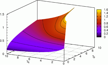
Figure 1: Mean-square fluctuation of the coordinate at t= 0𝑡 0t\,{=}\,0 as a function of both γqsubscript𝛾𝑞\gamma_{q} and γpsubscript𝛾𝑝\gamma_{p}, for τD= 0.01subscript𝜏D0.01\tau_{{}_{\rm{D}}}\,{=}\,0.01.
Refer to caption
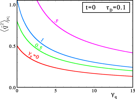
Figure 2: Mean-square fluctuation of the coordinate at t= 0𝑡 0t\,{=}\,0 as a function of γqsubscript𝛾𝑞\gamma_{q} for fixed values of γpsubscript𝛾𝑝\gamma_{p}. As in the case of standard dissipation, γp= 0subscript𝛾𝑝 0\gamma_{p}\,{=}\,0, the effect of increasing the intensity of the coordinate coupling is a decrease of q^2delimited-⟨⟩superscript^𝑞2\langle{\hat{q}^{2}}\rangle.
Refer to caption
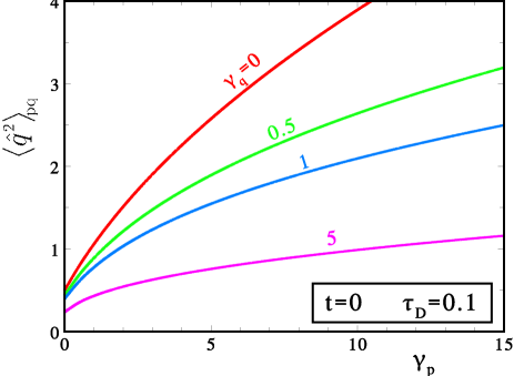
Figure 3: Mean-square fluctuation of the coordinate at t= 0𝑡 0t\,{=}\,0 as a function of γpsubscript𝛾𝑝\gamma_{p} for fixed values of γqsubscript𝛾𝑞\gamma_{q}. As in the case of anomalous dissipation, γq= 0subscript𝛾𝑞 0\gamma_{q}\,{=}\,0, the effect of increasing the intensity of the momentum coupling is an increase of q^2delimited-⟨⟩superscript^𝑞2\langle{\hat{q}^{2}}\rangle.

In the general case Eq. (19) has to be evaluated numerically. This is what we have done and Fig. 1 shows the three-dimensional resulting plot for α(0,γp,γq,τD=0.01)𝛼0subscript𝛾𝑝subscript𝛾𝑞subscript𝜏D0.01\alpha(0,\gamma_{p},\gamma_{q},\tau_{{}_{\rm{D}}}{=}0.01); its shape gives an overall idea of the combined effect of two baths. However, in order to highlight some important features which are barely apparent, it is necessary to analyze its cross-sections.

In Fig. 2 we first consider how α𝛼\alpha varies while increasing the coordinate coupling γqsubscript𝛾𝑞\gamma_{q}: also for nonzero γpsubscript𝛾𝑝\gamma_{p} the effect is a decrease of α𝛼\alpha, as if the q𝑞q-bath were a position measuring device, causing localization of the particle. From the same figure, and more clearly from Fig. 3, the complementary interpretation can be given to the action of the p𝑝p-bath, generalizing the observations made in the case of anomalous dissipation CFTV2001 ; AnkerholdP2007 ; note, however, that as soon as γqsubscript𝛾𝑞\gamma_{q} is switched on the steepness of the rise of α𝛼\alpha is considerably suppressed.

Given the opposite effect of the two baths, it is natural to ask what the result will be when both have equal strength, γp=γqsubscript𝛾𝑝subscript𝛾𝑞\gamma_{p}=\gamma_{q}: this is a nontrivial issue, especially from the point of view of the application to real problems where the canonical variables play symmetric roles, as mentioned in the Introduction.
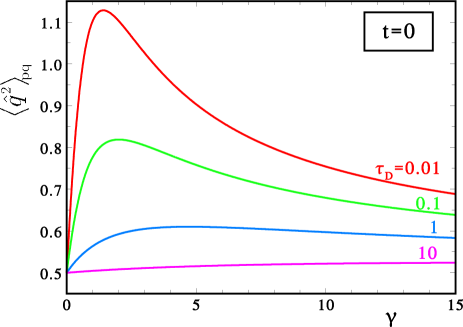
Refer to caption
Figure 4: Mean-square fluctuation of the coordinate at t= 0𝑡 0t\,{=}\,0 as a function of γ=γq=γp𝛾subscript𝛾𝑞subscript𝛾𝑝\gamma\,{=}\,\gamma_{q}\,{=}\,\gamma_{p}, i.e., for equally acting environments, for selected values of the Drude time τDsubscript𝜏D\tau_{{}_{\rm{D}}}. It appears that between the competing effects of the two baths, the prevailing one is that of increasing q^2delimited-⟨⟩superscript^𝑞2\langle{\hat{q}^{2}}\rangle; however, as the coupling intensity increases a maximum is reached and followed by a slow decrease towards the isolated-oscillator value.
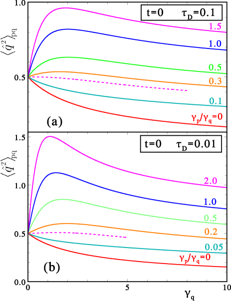
Refer to caption
Figure 5: Mean-square fluctuation of the coordinate for τD= 0.1subscript𝜏D0.1\tau_{{}_{\rm{D}}}\,{=}\,0.1 (a) and τD= 0.01subscript𝜏D0.01\tau_{{}_{\rm{D}}}\,{=}\,0.01 (b) at t= 0𝑡 0t\,{=}\,0 along the line γp=cγqsubscript𝛾𝑝𝑐subscript𝛾𝑞\gamma_{p}\,{=}\,c\,\gamma_{q} as a function of γqsubscript𝛾𝑞\gamma_{q}, for different values of c𝑐c. The dashed line, for c= 0.2214𝑐0.2214c{=}\,0.2214 in (a) and c= 0.1193𝑐0.1193c{=}\,0.1193 in (b), separates the decreasing from the nonmonotonic behaviors.
Refer to caption
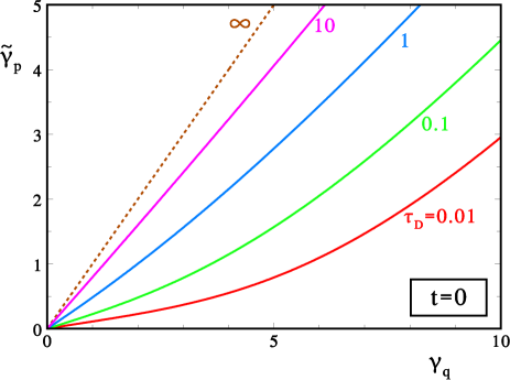
Figure 6: The function γ~p(γq)subscript~𝛾𝑝subscript𝛾𝑞\tilde{\gamma}_{p}(\gamma_{q}) corresponding to the cancelation of the competing effects of the two baths, so that the mean-square fluctuation of the coordinate keeps the isolated system’s value. The curves refer to t= 0𝑡 0t\,{=}\,0, so q^2=1/2delimited-⟨⟩superscript^𝑞212\langle{\hat{q}^{2}}\rangle=1/2, and to selected values of the Drude time τDsubscript𝜏D\tau_{{}_{\rm{D}}}.

The answer is given by the curves reported in Fig. 4: α=q^2pq𝛼subscriptdelimited-⟨⟩superscript^𝑞2pq\alpha=\big{\langle}{\hat{q}^{2}}\big{\rangle}_{\rm{pq}} is larger compared to the isolated oscillator, i.e., the quantum fluctuations of both canonical variables are enhanced by a symmetric environmental coupling. However, an unexpected behavior shows up while rising the intensity of the environmental coupling: after an initial rise the mean-square fluctuation shows a maximum, whose location and intensity depends upon the Drude memory time, and eventually slowly decreases back towards the isolated oscillator value α=1/2𝛼12\alpha=1/2.

It is obvious that, as the size of the zero-temperature fluctuations is affected by the mechanism of environmental coupling, one could formally modulate its intensity γ𝛾\gamma to drive through a quantum phase transition (QPT) a system that is close to it. At difference with standard dissipative systems, e.g., resistively shunted Josephson junction arrays, where a stronger dissipation leads towards the ‘ordered’ (superconducting) phase Fisher1987 , in the generalized case a higher γ𝛾\gamma would most commonly increase disorder. One can also speculate about the fact that the nonmonotonicity displayed in Fig. 4 opens the possibility to observe reentrant behavior around a QPT, namely by further rising γ𝛾\gamma beyond the critical value one could observe the restoration of the isolated-system’s ordered phase.

Having ascertained that the combined effect of the two baths is opposite to that of the single q𝑞q-bath, it is natural to look for the evolution one observes by gradually switching the p𝑝p-bath coupling on. In Figs. 5 the behavior of α𝛼\alpha is followed along straight lines in the plane (γq,γp)subscript𝛾𝑞subscript𝛾𝑝(\gamma_{q},\gamma_{p}), i.e., for fixed ratios c=γp/γq𝑐subscript𝛾𝑝subscript𝛾𝑞c=\gamma_{p}/\gamma_{q} between the intensities of the two environmental couplings. These figures, which differ for the choice of the Drude time, are essentially similar and display the competing interplay between the intensities of the environmental couplings for q𝑞q and p𝑝p: if the latter is small enough, the quenching effect of the former prevails. Increasing γpsubscript𝛾𝑝\gamma_{p} for any fixed γqsubscript𝛾𝑞\gamma_{q}, α𝛼\alpha must cross the isolated-system value α=1/2𝛼12\alpha=1/2 for some γ~psubscript~𝛾𝑝\tilde{\gamma}_{p}: along the line γ~p(γq)subscript~𝛾𝑝subscript𝛾𝑞\tilde{\gamma}_{p}(\gamma_{q}) the competing effects cancel each other and the mean-square fluctuation of the coordinate is stationary; since α>1/2𝛼12\alpha>1/2 for γp=γqsubscript𝛾𝑝subscript𝛾𝑞\gamma_{p}=\gamma_{q} it follows that γ~p(γq)<γqsubscript~𝛾𝑝subscript𝛾𝑞subscript𝛾𝑞\tilde{\gamma}_{p}(\gamma_{q})<\gamma_{q}. From Eq. (19) one can analytically obtain the initial slope of these curves as a function of the Drude memory time τDsubscript𝜏D\tau_{{}_{\rm{D}}},

γ~p(0)=2πτD4τD2lnτD+2τD2+πτD34lnτD2+3πτD2τD2+πτD3,superscriptsubscript~𝛾𝑝02𝜋subscript𝜏D4superscriptsubscript𝜏D2subscript𝜏D2superscriptsubscript𝜏D2𝜋superscriptsubscript𝜏D34subscript𝜏D23𝜋subscript𝜏D2superscriptsubscript𝜏D2𝜋superscriptsubscript𝜏D3\tilde{\gamma}_{p}^{\prime}(0)=\frac{2-\pi\tau_{{}_{\rm{D}}}-4\tau_{{}_{\rm{D}}}^{2}\ln\tau_{{}_{\rm{D}}}+2\tau_{{}_{\rm{D}}}^{2}+\pi\tau_{{}_{\rm{D}}}^{3}}{-4\ln\tau_{{}_{\rm{D}}}-2+3\pi\tau_{{}_{\rm{D}}}-2\tau_{{}_{\rm{D}}}^{2}+\pi\tau_{{}_{\rm{D}}}^{3}}~{}, (23)

which turns out to vanish in the Ohmic limit and tends to 1 for large τDsubscript𝜏D\tau_{{}_{\rm{D}}}. This is in agreement with the numerical calculation of γ~p(γq)subscript~𝛾𝑝subscript𝛾𝑞\tilde{\gamma}_{p}(\gamma_{q}) reported in Fig. 6.

Fig. 5 also suggests that, keeping the ratio c=γp/γq𝑐subscript𝛾𝑝subscript𝛾𝑞c={\gamma_{p}}/{\gamma_{q}} fixed, for large coupling intensity q^2delimited-⟨⟩superscript^𝑞2\langle{\hat{q}^{2}}\rangle tends to a finite value; one can indeed find that

q^212c=12γpγq.delimited-⟨⟩superscript^𝑞212𝑐12subscript𝛾𝑝subscript𝛾𝑞\langle{\hat{q}^{2}}\rangle\to\frac{1}{2}~{}\sqrt{c}=\frac{1}{2}~{}\sqrt{\frac{\gamma_{p}}{\gamma_{q}}}~{}. (24)

Substantially, it turns out that, after a possible initial increase of the spread of one of the canonical variables when the interaction is switched on, a very strong environmental coupling eventually tends to localize again both p^^𝑝\hat{p} and q^^𝑞\hat{q}, as the above limit also entails that

p^212γqγp;delimited-⟨⟩superscript^𝑝212subscript𝛾𝑞subscript𝛾𝑝\langle{\hat{p}^{2}}\rangle\to\frac{1}{2}~{}\sqrt{\frac{\gamma_{q}}{\gamma_{p}}}~{}; (25)

the shrinking of the fluctuations is visibly more effective for the variable with larger bath-coupling strength, but the product of the fluctuations obeys the constraint of the uncertainty principle,

q^2p^214.delimited-⟨⟩superscript^𝑞2delimited-⟨⟩superscript^𝑝214\langle{\hat{q}^{2}}\rangle\langle{\hat{p}^{2}}\rangle\to\frac{1}{4}~{}. (26)

In other words, a very large environmental coupling leads to a situation where the uncertainty is squeezed along one axis in the p𝑝p-q𝑞q plane with respect to the symmetric spread in the free system.
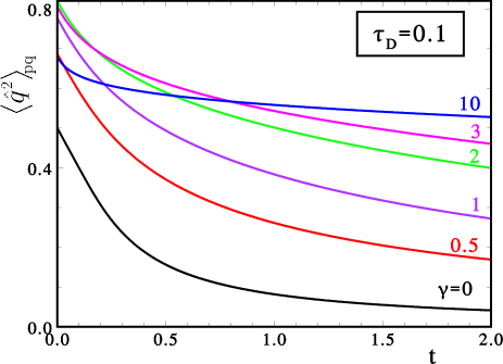
Refer to caption
Figure 7: Pure-quantum mean-square fluctuation of the coordinate for τD= 0.1subscript𝜏D0.1\tau_{{}_{\rm{D}}}\,{=}\,0.1 and different values of γ=γq=γp𝛾subscript𝛾𝑞subscript𝛾𝑝\gamma\,{=}\,\gamma_{q}\,{=}\,\gamma_{p} (i.e., for equally acting environments) as a function of t𝑡t.
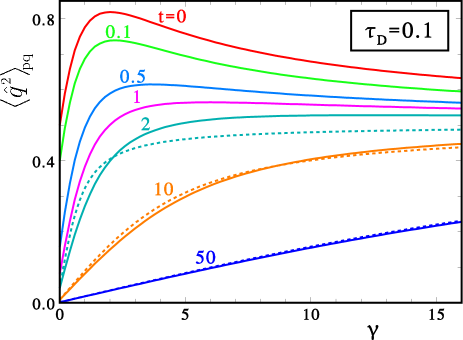
Refer to caption
Figure 8: Pure-quantum mean-square fluctuation of the coordinate at different temperatures as a function of γ=γq=γp𝛾subscript𝛾𝑞subscript𝛾𝑝\gamma\,{=}\,\gamma_{q}\,{=}\,\gamma_{p}, for τD=0.1subscript𝜏D0.1\tau_{{}_{\rm{D}}}=0.1. The dashed curves for t 2𝑡2t\,{\geq}\,2 represent the large-t𝑡t analytic approximation (27) valid for t1/(2πτD)1.6much-greater-than𝑡12𝜋subscript𝜏Dsimilar-to-or-equals1.6t\gg 1/(2\pi\tau_{{}_{\rm{D}}})\simeq 1.6.

II.2.2 Finite temperature

As Eq. (17) shows, the effect of environmental coupling only affects the purely quantum part of the fluctuations, which decreases with increasing temperature: so, one expects a softening of the effects observed at zero-T𝑇T when T𝑇T rises. However, the fate of the reentrant fluctuation amplitude displayed in Figs. 4 and 5 is not obvious. To unveil such issue we plot in Fig. 7 the behavior of α=q^2pq𝛼subscriptdelimited-⟨⟩superscript^𝑞2pq\alpha=\langle{\hat{q}^{2}}\rangle_{\rm{pq}} vs temperature for the situation of equally acting environments. It appears that a stronger environmental coupling weakens the decrease of q^2pqsubscriptdelimited-⟨⟩superscript^𝑞2pq\langle{\hat{q}^{2}}\rangle_{\rm{pq}} with temperature, and that for t 1greater-than-or-equivalent-to𝑡1t\,{\gtrsim}\,1 a monotonic behavior is apparently restored. This fact is more evident by looking at the curves for increasing temperatures reported in Fig. 8.

When the temperature is larger than the Drude cutoff frequency, t1/(2πτD)much-greater-than𝑡12𝜋subscript𝜏Dt\gg 1/(2\pi\tau_{{}_{\rm{D}}}), the expressions (18) for the kernels can be well approximated by their asymptotic values kqnγq/τDsimilar-to-or-equalssubscript𝑘𝑞𝑛subscript𝛾𝑞subscript𝜏Dk_{qn}\simeq\gamma_{q}/\tau_{{}_{\rm{D}}} and kpnγp/τDsimilar-to-or-equalssubscript𝑘𝑝𝑛subscript𝛾𝑝subscript𝜏Dk_{pn}\simeq\gamma_{p}/\tau_{{}_{\rm{D}}}, so their dependence on n𝑛n disappears and the summation (17) becomes analytic,

αcp2cq(cothcpcq2t2tcpcq)similar-to-or-equals𝛼subscript𝑐𝑝2subscript𝑐𝑞hyperbolic-cotangentsubscript𝑐𝑝subscript𝑐𝑞2𝑡2𝑡subscript𝑐𝑝subscript𝑐𝑞\alpha\simeq\frac{c_{p}}{2c_{q}}\Big{(}\coth\frac{c_{p}c_{q}}{2t}-\frac{2t}{c_{p}c_{q}}\Big{)} (27)

with cp,q2=1+γp,q/τDsuperscriptsubscript𝑐𝑝𝑞21subscript𝛾𝑝𝑞subscript𝜏Dc_{p,q}^{2}=1+\gamma_{p,q}/\tau_{{}_{\rm{D}}}: this approximation is shown as dashed lines in Fig. 8; for cpcq/2t 1much-greater-thansubscript𝑐𝑝subscript𝑐𝑞2𝑡1c_{p}c_{q}/{2t}\,{\gg}\,1, i.e., under the combined condition γpγq2τDt1/πmuch-greater-thansubscript𝛾𝑝subscript𝛾𝑞2subscript𝜏D𝑡much-greater-than1𝜋\sqrt{\gamma_{p}\gamma_{q}}\gg 2\tau_{{}_{\rm{D}}}t\gg 1/\pi, the value of α𝛼\alpha tends to the constant cp/2cqsubscript𝑐𝑝2subscript𝑐𝑞{c_{p}}/{2c_{q}}. As the validity of this approximation entails the disappearance of the maximum, the nonmonotonic behavior is expected for t 1/(2πτD)less-than-or-similar-to𝑡12𝜋subscript𝜏Dt\,{\lesssim}\,1/(2\pi\tau_{{}_{\rm{D}}}).

III Coordinate and momentum coupled with a single environment

It can also happen that there is one single environment coupled with both canonical variables: the most general influence Hamiltonian can be found in Ref. KohlerS2006 . However, there are two main scenarios of physical relevance: the first occurs when both q^^𝑞\hat{q} and p^^𝑝\hat{p} are coupled with the same bath variables (say, the coordinates), while in the second the qαsubscript𝑞𝛼q_{\alpha}’s are coupled with q^^𝑞\hat{q} and the pαsubscript𝑝𝛼p_{\alpha}’s with p^^𝑝\hat{p}. The first scenario has a realization in the coupling of spins with lattice vibrations due to their modulation of the exchange integral; in the second case a natural model could be a spin-orbit interaction where the orbital angular momenta are thermalized by lattice vibrations.

III.1 System coupled with bath coordinates

Starting from the coupling Hamiltonian,

^I=12α[aα2p^α2+bα2(q^αcαq^dαp^)2],subscript^I12subscript𝛼delimited-[]superscriptsubscript𝑎𝛼2superscriptsubscript^𝑝𝛼2superscriptsubscript𝑏𝛼2superscriptsubscript^𝑞𝛼subscript𝑐𝛼^𝑞subscript𝑑𝛼^𝑝2\hat{\cal{H}}_{\rm{I}}=\frac{1}{2}\sum_{\alpha}\big{[}a_{\alpha}^{2}\hat{p}_{\alpha}^{2}+b_{\alpha}^{2}(\hat{q}_{\alpha}-c_{\alpha}\hat{q}-d_{\alpha}\hat{p})^{2}\big{]}~{}, (28)

we get the influence action:

𝒮I[p,q]=β2n[kqnqnqn+kpnpnpn+2κnpnqn],subscript𝒮I𝑝𝑞𝛽2subscript𝑛delimited-[]subscript𝑘𝑞𝑛subscript𝑞𝑛subscript𝑞𝑛subscript𝑘𝑝𝑛subscript𝑝𝑛subscript𝑝𝑛2subscript𝜅𝑛subscript𝑝𝑛subscript𝑞𝑛{\cal{S}}_{\rm{I}}[p,q]=-\frac{\beta}{2}\,\sum_{n}\big{[}k_{qn}~{}q_{n}q_{-n}+k_{pn}~{}p_{n}p_{-n}+2\kappa_{n}p_{n}q_{-n}\big{]}~{}, (29)

with the kernels

kqn=αbα2cα2νn2νn2+ωα2,kpn=αbα2dα2νn2νn2+ωα2,formulae-sequencesubscript𝑘𝑞𝑛subscript𝛼superscriptsubscript𝑏𝛼2superscriptsubscript𝑐𝛼2superscriptsubscript𝜈𝑛2superscriptsubscript𝜈𝑛2superscriptsubscript𝜔𝛼2subscript𝑘𝑝𝑛subscript𝛼superscriptsubscript𝑏𝛼2superscriptsubscript𝑑𝛼2superscriptsubscript𝜈𝑛2superscriptsubscript𝜈𝑛2superscriptsubscript𝜔𝛼2k_{qn}=\sum_{\alpha}\frac{b_{\alpha}^{2}c_{\alpha}^{2}\nu_{n}^{2}}{\nu_{n}^{2}+\omega_{\alpha}^{2}}~{},~{}~{}~{}~{}k_{pn}=\sum_{\alpha}\frac{b_{\alpha}^{2}d_{\alpha}^{2}\nu_{n}^{2}}{\nu_{n}^{2}+\omega_{\alpha}^{2}}~{}, (30)
κn=αbα2cαdανn2νn2+ωα2.subscript𝜅𝑛subscript𝛼superscriptsubscript𝑏𝛼2subscript𝑐𝛼subscript𝑑𝛼superscriptsubscript𝜈𝑛2superscriptsubscript𝜈𝑛2superscriptsubscript𝜔𝛼2\kappa_{n}=\sum_{\alpha}\frac{b_{\alpha}^{2}c_{\alpha}d_{\alpha}\nu_{n}^{2}}{\nu_{n}^{2}+\omega_{\alpha}^{2}}~{}. (31)

It is immediate to check that the last kernel vanishes if cαdα=0subscript𝑐𝛼subscript𝑑𝛼0c_{\alpha}{d_{\alpha}}=0 for any α𝛼\alpha, yielding the previous Eq. (7): indeed, if the coefficients cαsubscript𝑐𝛼c_{\alpha} and dαsubscript𝑑𝛼d_{\alpha} are not simultaneously nonzero, the bath can be split into two independent baths and the two-bath case studied in the previous sections is recovered.

In the case when all the coefficients cαsubscript𝑐𝛼c_{\alpha} and dαsubscript𝑑𝛼d_{\alpha} are positive the spectral density Weiss2008 Jpq(ω)subscript𝐽𝑝𝑞𝜔J_{pq}(\omega) for κnsubscript𝜅𝑛\kappa_{n}, such that

κn=2νn20𝑑ωJpq(ω)ω2+νn2,subscript𝜅𝑛2superscriptsubscript𝜈𝑛2superscriptsubscript0differential-d𝜔subscript𝐽𝑝𝑞𝜔superscript𝜔2superscriptsubscript𝜈𝑛2\kappa_{n}=2\nu_{n}^{2}\int_{0}^{\infty}d\omega\frac{J_{pq}(\omega)}{\omega^{2}+\nu_{n}^{2}}~{}, (32)

can be expressed in terms of those for the first two kernels,

Jq(ω)subscript𝐽𝑞𝜔\displaystyle J_{q}(\omega) \displaystyle\equiv αbα2cα2ωαδ(ω2ωα2),subscript𝛼superscriptsubscript𝑏𝛼2subscriptsuperscript𝑐2𝛼subscript𝜔𝛼𝛿superscript𝜔2superscriptsubscript𝜔𝛼2\displaystyle\sum_{\alpha}b_{\alpha}^{2}c^{2}_{\alpha}\omega_{\alpha}\,\delta(\omega^{2}{-}\omega_{\alpha}^{2})~{},
Jp(ω)subscript𝐽𝑝𝜔\displaystyle J_{p}(\omega) \displaystyle\equiv αbα2dα2ωαδ(ω2ωα2),subscript𝛼superscriptsubscript𝑏𝛼2subscriptsuperscript𝑑2𝛼subscript𝜔𝛼𝛿superscript𝜔2superscriptsubscript𝜔𝛼2\displaystyle\sum_{\alpha}b_{\alpha}^{2}d^{2}_{\alpha}\omega_{\alpha}\,\delta(\omega^{2}{-}\omega_{\alpha}^{2})~{}, (33)

as their geometric average as their geometric average KohlerS2006

Jpq(ω)=Jq(ω)Jp(ω).subscript𝐽𝑝𝑞𝜔subscript𝐽𝑞𝜔subscript𝐽𝑝𝜔J_{pq}(\omega)=\sqrt{J_{q}(\omega)\,J_{p}(\omega)}~{}. (34)

The baths are independent if the supports of Jq(ω)subscript𝐽𝑞𝜔J_{q}(\omega) and Jp(ω)subscript𝐽𝑝𝜔J_{p}(\omega) have no intersection, i.e., if Jpq(ω)subscript𝐽𝑝𝑞𝜔J_{pq}(\omega) vanishes for any ω𝜔\omegafootnote

Eventually, using the result of Appendix B, the expressions for the fluctuations in the case of the bath coupling (28) are found,

𝒵=1βω0n=1νn2νn2+(a2+kpn)(b2+kqn)κn2,𝒵1𝛽subscript𝜔0superscriptsubscriptproduct𝑛1superscriptsubscript𝜈𝑛2superscriptsubscript𝜈𝑛2superscript𝑎2subscript𝑘𝑝𝑛superscript𝑏2subscript𝑘𝑞𝑛superscriptsubscript𝜅𝑛2{\cal{Z}}=\frac{1}{\beta\omega_{0}}\prod_{n=1}^{\infty}\frac{\nu_{n}^{2}}{\nu_{n}^{2}+(a^{2}{+}k_{pn})(b^{2}{+}k_{qn})-\kappa_{n}^{2}}, (35)
p^2pq=2βn=1b2+kqnνn2+(a2+kpn)(b2+kqn)κn2,subscriptdelimited-⟨⟩superscript^𝑝2pq2𝛽superscriptsubscript𝑛1superscript𝑏2subscript𝑘𝑞𝑛superscriptsubscript𝜈𝑛2superscript𝑎2subscript𝑘𝑝𝑛superscript𝑏2subscript𝑘𝑞𝑛superscriptsubscript𝜅𝑛2\displaystyle\big{\langle}{\hat{p}^{2}}\big{\rangle}_{\rm{pq}}=\frac{2}{\beta}\sum_{n=1}^{\infty}\frac{b^{2}{+}k_{qn}}{\nu_{n}^{2}+(a^{2}{+}k_{pn})(b^{2}{+}k_{qn})-\kappa_{n}^{2}}~{}, (36)
q^2pq=2βn=1a2+kpnνn2+(a2+kpn)(b2+kqn)κn2,subscriptdelimited-⟨⟩superscript^𝑞2pq2𝛽superscriptsubscript𝑛1superscript𝑎2subscript𝑘𝑝𝑛superscriptsubscript𝜈𝑛2superscript𝑎2subscript𝑘𝑝𝑛superscript𝑏2subscript𝑘𝑞𝑛superscriptsubscript𝜅𝑛2\displaystyle\big{\langle}{\hat{q}^{2}}\big{\rangle}_{\rm{pq}}=\frac{2}{\beta}\sum_{n=1}^{\infty}\frac{a^{2}{+}k_{pn}}{\nu_{n}^{2}+(a^{2}{+}k_{pn})(b^{2}{+}k_{qn})-\kappa_{n}^{2}},
p^q^+q^p^pq=4βn=1κnνn2+(a2+kpn)(b2+kqn)κn2.subscriptdelimited-⟨⟩^𝑝^𝑞^𝑞^𝑝pq4𝛽superscriptsubscript𝑛1subscript𝜅𝑛superscriptsubscript𝜈𝑛2superscript𝑎2subscript𝑘𝑝𝑛superscript𝑏2subscript𝑘𝑞𝑛superscriptsubscript𝜅𝑛2\displaystyle\big{\langle}{\hat{p}\hat{q}+\hat{q}\hat{p}}\big{\rangle}_{\rm{pq}}=-\frac{4}{\beta}\sum_{n=1}^{\infty}\frac{\kappa_{n}}{\nu_{n}^{2}+(a^{2}{+}k_{pn})(b^{2}{+}k_{qn})-\kappa_{n}^{2}}~{}.

As Eqs. (30) and (31) imply the inequality kqnkpnκn2subscript𝑘𝑞𝑛subscript𝑘𝑝𝑛superscriptsubscript𝜅𝑛2k_{qn}k_{pn}\geq\kappa_{n}^{2}, it follows that the denominators are always positive. Note that if the bath is coupled to the variable p^±q^plus-or-minus^𝑝^𝑞\hat{p}\pm\hat{q} (i.e., cα=±dαsubscript𝑐𝛼plus-or-minussubscript𝑑𝛼c_{\alpha}={\pm}d_{\alpha}), then ±κn=kpn=kqn>0plus-or-minussubscript𝜅𝑛subscript𝑘𝑝𝑛subscript𝑘𝑞𝑛0\pm\kappa_{n}=k_{pn}=k_{qn}>0: from the above variances it follows then that p^±q^plus-or-minus^𝑝^𝑞\hat{p}\pm\hat{q} becomes smaller (larger) when the environmental coupling is switched on,

(p^±q^)2pq=2βn=1a2+b2+(kpn+kqn2κn)νn2+(a2+kpn)(b2+kqn)κn2,subscriptdelimited-⟨⟩superscriptplus-or-minus^𝑝^𝑞2pq2𝛽superscriptsubscript𝑛1superscript𝑎2superscript𝑏2minus-or-plussubscript𝑘𝑝𝑛subscript𝑘𝑞𝑛2subscript𝜅𝑛superscriptsubscript𝜈𝑛2superscript𝑎2subscript𝑘𝑝𝑛superscript𝑏2subscript𝑘𝑞𝑛superscriptsubscript𝜅𝑛2\big{\langle}{(\hat{p}\pm\hat{q})^{2}}\big{\rangle}_{\rm{pq}}=\frac{2}{\beta}\sum_{n=1}^{\infty}\frac{a^{2}+b^{2}{+}(k_{pn}+k_{qn}\mp 2\kappa_{n})}{\nu_{n}^{2}+(a^{2}{+}k_{pn})(b^{2}{+}k_{qn})-\kappa_{n}^{2}}~{}, (37)

which corresponds to a squeezed Gaussian distribution along a diagonal in the p𝑝p-q𝑞q plane, in agreement with the Heisenberg uncertainty relation. This observation also confirms the overall picture that the environment acts as a measuring device for whatever variable it is coupled with.

Let us consider now a phenomenological guess fo the first two kernels (30), while the third one, κnsubscript𝜅𝑛\kappa_{n}, follows from Eqs. (32)–(34). Taking Drude kernels with equal memory times τDsubscript𝜏D\tau_{{}_{\rm{D}}} as in Eq. (15), corresponding to the spectral densities

Jp,q(ω)=γp,qπ11+τD2ω2,subscript𝐽𝑝𝑞𝜔subscript𝛾𝑝𝑞𝜋11superscriptsubscript𝜏D2superscript𝜔2J_{p,q}(\omega)=\frac{\gamma_{p,q}}{\pi}\,\frac{1}{1+\tau_{{}_{\rm{D}}}^{2}\omega^{2}}~{}, (38)

one simply finds

κn=γqγp|νn|1+τD|νn|;subscript𝜅𝑛subscript𝛾𝑞subscript𝛾𝑝subscript𝜈𝑛1subscript𝜏Dsubscript𝜈𝑛\kappa_{n}=\frac{\sqrt{\gamma_{q}\gamma_{p}}~{}|\nu_{n}|}{1+\tau_{{}_{\rm{D}}}\,|\nu_{n}|}~{}; (39)

in this case one exactly has κn2=kpnkqnsuperscriptsubscript𝜅𝑛2subscript𝑘𝑝𝑛subscript𝑘𝑞𝑛\kappa_{n}^{2}=k_{pn}k_{qn}, and in the dimensionless formulation introduced in Section II.2 the coordinate pure-quantum fluctuation is given by

α=2tn=11+kpn(2πtn)2+1+kpn+kqn,𝛼2𝑡superscriptsubscript𝑛11subscript𝑘𝑝𝑛superscript2𝜋𝑡𝑛21subscript𝑘𝑝𝑛subscript𝑘𝑞𝑛\alpha=2t\sum_{n=1}^{\infty}\frac{1+k_{pn}}{(2\pi{t}n)^{2}+1+k_{pn}+k_{qn}}~{}, (40)

with the kernels given in Eq. (18). For t=0𝑡0t=0 it becomes the integral

α(0,γp,γq,τD)=0dxπ1+γpg(x)x2+1+(γp+γq)g(x),𝛼0subscript𝛾𝑝subscript𝛾𝑞subscript𝜏Dsuperscriptsubscript0𝑑𝑥𝜋1subscript𝛾𝑝𝑔𝑥superscript𝑥21subscript𝛾𝑝subscript𝛾𝑞𝑔𝑥\alpha(0,\gamma_{p},\gamma_{q},\tau_{{}_{\rm{D}}})=\int_{0}^{\infty}\frac{dx}{\pi}\,\frac{1+\gamma_{p}\,g(x)}{\,x^{2}+1{+}(\gamma_{p}{+}\gamma_{q})\,g(x)}~{}, (41)

with g(x)𝑔𝑥g(x) as in Eq. (20).

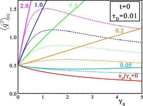
In Fig. 9 it appears indeed that the mean-square fluctuation of the coordinate is enhanced by the coupling mechanism considered in this case, a result of the ‘diagonal squeezing’ discussed after Eq. (37). Of course, different distributions of the coefficients cαsubscript𝑐𝛼c_{\alpha} and dαsubscript𝑑𝛼d_{\alpha} can yield a less dramatic increase with the environmental coupling strength.
Refer to caption
Figure 9: System coupled with the bath coordinates. Mean-square fluctuation of the coordinate, Eq. (40), at t= 0𝑡 0t\,{=}\,0 along the line γp=cγqsubscript𝛾𝑝𝑐subscript𝛾𝑞\gamma_{p}\,{=}\,c\,\gamma_{q} as a function of γqsubscript𝛾𝑞\gamma_{q}, for different values of c𝑐c. The dashed lines correspond to the curves for the two-bath case of Fig. 5 (b).

III.2 System coupled with bath coordinates and momenta

In this case the most general interaction Hamiltonian would take the form

^I=12α[aα2(p^αcαp^)2+bα2(q^αcαq^)2];subscript^I12subscript𝛼delimited-[]superscriptsubscript𝑎𝛼2superscriptsubscript^𝑝𝛼subscript𝑐𝛼^𝑝2superscriptsubscript𝑏𝛼2superscriptsubscript^𝑞𝛼subscript𝑐𝛼^𝑞2\hat{\cal{H}}_{\rm{I}}=\frac{1}{2}\sum_{\alpha}\big{[}a_{\alpha}^{2}(\hat{p}_{\alpha}-c_{\alpha}\hat{p})^{2}+b_{\alpha}^{2}(\hat{q}_{\alpha}-c_{\alpha}\hat{q})^{2}\big{]}~{}; (42)

note that in this case the coefficients cαsubscript𝑐𝛼c_{\alpha} cannot be absorbed by means of linear canonical transformations of the bath variables.

The calculation of the influence action leads to an expression similar to Eq. (7), but for the appearance of an antisymmetric correlation kernel νnκ~nsubscript𝜈𝑛subscript~𝜅𝑛\nu_{n}\tilde{\kappa}_{n},

𝒮I[p,q]=β2n(kpnpnpn+kqnqnqn+2νnκ~npnqn),subscript𝒮I𝑝𝑞𝛽2subscript𝑛subscript𝑘𝑝𝑛subscript𝑝𝑛subscript𝑝𝑛subscript𝑘𝑞𝑛subscript𝑞𝑛subscript𝑞𝑛2subscript𝜈𝑛subscript~𝜅𝑛subscript𝑝𝑛subscript𝑞𝑛{\cal{S}}_{\rm{I}}[p,q]=-\frac{\beta}{2}\sum_{n}\big{(}k_{pn}p_{n}p_{-n}+k_{qn}q_{n}q_{-n}+2\nu_{n}\tilde{\kappa}_{n}p_{n}q_{-n}\big{)},~{} (43)

with the Matsubara components

kqn=αcα2bα2νn2νn2+ωα2,kpn=αcα2aα2νn2νn2+ωα2,formulae-sequencesubscript𝑘𝑞𝑛subscript𝛼superscriptsubscript𝑐𝛼2superscriptsubscript𝑏𝛼2superscriptsubscript𝜈𝑛2superscriptsubscript𝜈𝑛2superscriptsubscript𝜔𝛼2subscript𝑘𝑝𝑛subscript𝛼superscriptsubscript𝑐𝛼2superscriptsubscript𝑎𝛼2superscriptsubscript𝜈𝑛2superscriptsubscript𝜈𝑛2superscriptsubscript𝜔𝛼2k_{qn}=\sum_{\alpha}\frac{c_{\alpha}^{2}b_{\alpha}^{2}\nu_{n}^{2}}{\nu_{n}^{2}+\omega_{\alpha}^{2}}~{},~{}~{}~{}~{}k_{pn}=\sum_{\alpha}\frac{c_{\alpha}^{2}a_{\alpha}^{2}\nu_{n}^{2}}{\nu_{n}^{2}+\omega_{\alpha}^{2}}~{}, (44)
κ~n=αcα2ωα2νn2+ωα2.subscript~𝜅𝑛subscript𝛼superscriptsubscript𝑐𝛼2superscriptsubscript𝜔𝛼2superscriptsubscript𝜈𝑛2superscriptsubscript𝜔𝛼2\tilde{\kappa}_{n}=\sum_{\alpha}\frac{c_{\alpha}^{2}\omega_{\alpha}^{2}}{\nu_{n}^{2}+\omega_{\alpha}^{2}}~{}. (45)

Using the result of Appendix B one has the expressions for the partition function and the mean-square fluctuations:

𝒵=1βω0n=1νn2νn2(1+κ~n)2+(a2+kpn)(b2+kqn),𝒵1𝛽subscript𝜔0superscriptsubscriptproduct𝑛1superscriptsubscript𝜈𝑛2superscriptsubscript𝜈𝑛2superscript1subscript~𝜅𝑛2superscript𝑎2subscript𝑘𝑝𝑛superscript𝑏2subscript𝑘𝑞𝑛{\cal{Z}}=\frac{1}{\beta\omega_{0}}\prod_{n=1}^{\infty}\frac{\nu_{n}^{2}}{\nu_{n}^{2}(1{+}\tilde{\kappa}_{n})^{2}+(a^{2}{+}k_{pn})(b^{2}{+}k_{qn})}~{}, (46)
p^2pqsubscriptdelimited-⟨⟩superscript^𝑝2pq\displaystyle\big{\langle}{\hat{p}^{2}}\big{\rangle}_{\rm{pq}} =\displaystyle= 2βn=1b2+kqnνn2(1+κ~n)2+(a2+kpn)(b2+kqn),2𝛽superscriptsubscript𝑛1superscript𝑏2subscript𝑘𝑞𝑛superscriptsubscript𝜈𝑛2superscript1subscript~𝜅𝑛2superscript𝑎2subscript𝑘𝑝𝑛superscript𝑏2subscript𝑘𝑞𝑛\displaystyle\frac{2}{\beta}\sum_{n=1}^{\infty}\frac{b^{2}+k_{qn}}{\nu_{n}^{2}(1{+}\tilde{\kappa}_{n})^{2}+(a^{2}{+}k_{pn})(b^{2}{+}k_{qn})}~{},
q^2pqsubscriptdelimited-⟨⟩superscript^𝑞2pq\displaystyle\big{\langle}{\hat{q}^{2}}\big{\rangle}_{\rm{pq}} =\displaystyle= 2βn=1a2+kpnνn2(1+κ~n)2+(a2+kpn)(b2+kqn),2𝛽superscriptsubscript𝑛1superscript𝑎2subscript𝑘𝑝𝑛superscriptsubscript𝜈𝑛2superscript1subscript~𝜅𝑛2superscript𝑎2subscript𝑘𝑝𝑛superscript𝑏2subscript𝑘𝑞𝑛\displaystyle\frac{2}{\beta}\sum_{n=1}^{\infty}\frac{a^{2}+k_{pn}}{\nu_{n}^{2}(1{+}\tilde{\kappa}_{n})^{2}{+}(a^{2}{+}k_{pn})(b^{2}{+}k_{qn})}\,,~{} (47)

while p^q^+q^p^=0delimited-⟨⟩^𝑝^𝑞^𝑞^𝑝0\langle{\hat{p}\hat{q}+\hat{q}\hat{p}}\rangle=0. Therefore, the kernel κ~nsubscript~𝜅𝑛\tilde{\kappa}_{n} has the effect to lower the fluctuations of both canonical variables with respect to the case of two independent baths. It is reasonable to use a phenomenological guess for kqnsubscript𝑘𝑞𝑛k_{qn} and kpnsubscript𝑘𝑝𝑛k_{pn}, while κ~nsubscript~𝜅𝑛\tilde{\kappa}_{n} is connected with them: in terms of the spectral densities it can be represented as

κ~n=20ωJq(ω)Jp(ω)ω2+νn2𝑑ω.subscript~𝜅𝑛2superscriptsubscript0𝜔subscript𝐽𝑞𝜔subscript𝐽𝑝𝜔superscript𝜔2superscriptsubscript𝜈𝑛2differential-d𝜔\tilde{\kappa}_{n}=2\int_{0}^{\infty}\frac{\omega\sqrt{J_{q}(\omega)\,J_{p}(\omega)}}{\omega^{2}+\nu_{n}^{2}}~{}d\omega~{}. (48)

Taking Drude kernels with equal memory times τDsubscript𝜏D\tau_{{}_{\rm{D}}} as in Eq. (15), corresponding to the spectral densities (38), one obtains

κ~n=γqγpf(τDνn),f(x)1πlnx2x21.formulae-sequencesubscript~𝜅𝑛subscript𝛾𝑞subscript𝛾𝑝𝑓subscript𝜏Dsubscript𝜈𝑛𝑓𝑥1𝜋superscript𝑥2superscript𝑥21\tilde{\kappa}_{n}=\sqrt{\gamma_{q}\gamma_{p}}~{}f(\tau_{{}_{\rm{D}}}\nu_{n})~{},~{}~{}~{}~{}~{}~{}f(x)\equiv\frac{1}{\pi}~{}\frac{\ln x^{2}}{x^{2}-1}~{}. (49)

Note that κ~nsubscript~𝜅𝑛\tilde{\kappa}_{n} is positive and that νnκ~n(lnn)/n0similar-tosubscript𝜈𝑛subscript~𝜅𝑛𝑛𝑛0\nu_{n}\tilde{\kappa}_{n}\sim(\ln{n})/n\to 0 for n𝑛n\to\infty. In the dimensionless formulation of Section II.2, with the kernels (18), the pure-quantum fluctuation of the coordinate reads

α=2tn=11+kpn(2πtn)2(1+κ~n)2+(1+kpn)(1+kqn),𝛼2𝑡superscriptsubscript𝑛11subscript𝑘𝑝𝑛superscript2𝜋𝑡𝑛2superscript1subscript~𝜅𝑛21subscript𝑘𝑝𝑛1subscript𝑘𝑞𝑛\alpha=2t\sum_{n=1}^{\infty}\frac{1+k_{pn}}{(2\pi{t}n)^{2}(1{+}\tilde{\kappa}_{n})^{2}+(1{+}k_{pn})(1{+}k_{qn})}~{}, (50)

with κ~n=γqγpf(2πtnτD)subscript~𝜅𝑛subscript𝛾𝑞subscript𝛾𝑝𝑓2𝜋𝑡𝑛subscript𝜏D\tilde{\kappa}_{n}=\sqrt{\gamma_{q}\gamma_{p}}~{}f(2\pi{t}n\tau_{{}_{\rm{D}}}). At zero temperature this becomes the integral

α(0,γp,γq,τD)=𝛼0subscript𝛾𝑝subscript𝛾𝑞subscript𝜏Dabsent\displaystyle\alpha(0,\gamma_{p},\gamma_{q},\tau_{{}_{\rm{D}}})= (51)
=0dxπ1+γpg(x)x2[1+κ~(x)]2+[1+γpg(x)][1+γqg(x)],absentsuperscriptsubscript0𝑑𝑥𝜋1subscript𝛾𝑝𝑔𝑥superscript𝑥2superscriptdelimited-[]1~𝜅𝑥2delimited-[]1subscript𝛾𝑝𝑔𝑥delimited-[]1subscript𝛾𝑞𝑔𝑥\displaystyle=\int_{0}^{\infty}\frac{dx}{\pi}\,\frac{1+\gamma_{p}\,g(x)}{x^{2}[1{+}\tilde{\kappa}(x)]^{2}+[1{+}\gamma_{p}\,g(x)][1{+}\gamma_{q}\,g(x)]}~{},

with κ~(x)=γqγpf(τDx)~𝜅𝑥subscript𝛾𝑞subscript𝛾𝑝𝑓subscript𝜏D𝑥\tilde{\kappa}(x)=\sqrt{\gamma_{q}\gamma_{p}}\,f(\tau_{{}_{\rm{D}}}x) and g(x)𝑔𝑥g(x) as in Eq. (20)

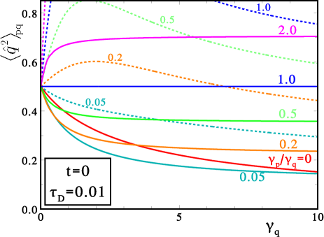
From Fig. 10 one can see that an environmental coupling of the kind of Eq. (42) produces much smaller effects than the previously considered ones. Note that the effect of increasing the bath-momentum coupling γpsubscript𝛾𝑝\gamma_{p} even initially shrinks the coordinate fluctuations, with a further slow rise. Moreover, it is particularly surprising to see that the existence of environmental coupling is irrelevant in the symmetric case; this means that the integral (51) sticks to the isolated system’s value 1/2121/2, whatever the values of γp=γqsubscript𝛾𝑝subscript𝛾𝑞\gamma_{p}\,{=}\,\gamma_{q} and τDsubscript𝜏D\tau_{{}_{\rm{D}}}: this result is far from being apparent from Eq. (51).
Refer to caption
Figure 10: System coupled with the bath coordinates and momenta. Mean-square fluctuation of the coordinate, Eq. (50), at t= 0𝑡 0t\,{=}\,0 along the line γp=cγqsubscript𝛾𝑝𝑐subscript𝛾𝑞\gamma_{p}\,{=}\,c\,\gamma_{q} as a function of γqsubscript𝛾𝑞\gamma_{q}, for different values of c𝑐c. The dashed lines correspond to the curves for the two-bath case of Fig. 5 (b).

IV Conclusions

Motivated by quest for a suitable description of spin-lattice coupling, with the lattice regarded as a harmonic bath of thermalized degrees of freedom, we considered a generalized system-plus-reservoir (SPR) model where both coordinates and momenta are subject to the interaction with the environment. While it was known that coupling a bath to a canonical variable quenches its fluctuations, attaching independent baths to both coordinate and momentum generally enhances their fluctuations. In the case of a spin system, such larger quantum fluctuations could open the possibility of reaching the quantum phase transition of the spin-1212\frac{1}{2} two-dimensional Heisenberg antiferromagnet ChakravartyHN1989 , i.e., spin-lattice coupling could yield a vanishing zero-T𝑇T sublattice magnetization with a power-law divergent correlation length. This possibility is to be further analyzed by a quantitatively accurate approach. Moreover and surprisingly, it turns out that the effect is nonmonotonic with the coupling strength, opening the possibility of a reentrant behavior in such a quantum critical system driven by its environmental coupling strength.

Other kinds of coupling involving both canonical variables and a single bath have been considered and briefly discussed. If the coupling terms do not simultaneously involve noncommuting bath variables (e.g., only bath coordinates) the result is a modification of the two-bath scenario with a further enhancement of the fluctuations and disappearance of the above mentioned nonmonotonicity. In the opposite case it clearly appears that the further ‘interference’ effect gives rise to generally smaller fluctuations, i.e., the intensity of bath-momentum coupling is much less effective in increasing the coordinate fluctuations, which moreover show two exotic features: a counterintuitive initial decrease when γpsubscript𝛾𝑝\gamma_{p} is switched on and the intriguing stability to the isolated system’s value in the symmetric case γp=γqsubscript𝛾𝑝subscript𝛾𝑞\gamma_{p}\,{=}\,\gamma_{q}; in other words, a symmetric environmental interaction appears to be ineffective for what attains mean square fluctuations.

Acknowledgements.
We thank Prof. Valerio Tognetti for stimulating us to further investigate these topics and for his useful suggestions.

Appendix A The standard system-plus-reservoir model

A bath attached to the coordinate q^^𝑞\hat{q} of the system of interest, e.g., the oscillator (1), is a collection of harmonic oscillators described by the Hamiltonian

^I=12α[aα2p^α2+bα2(q^αq^)2].subscript^I12subscript𝛼delimited-[]superscriptsubscript𝑎𝛼2superscriptsubscript^𝑝𝛼2superscriptsubscript𝑏𝛼2superscriptsubscript^𝑞𝛼^𝑞2\hat{\cal{H}}_{\rm{I}}=\frac{1}{2}\sum_{\alpha}\big{[}a_{\alpha}^{2}\hat{p}_{\alpha}^{2}+b_{\alpha}^{2}(\hat{q}_{\alpha}-\hat{q})^{2}\big{]}~{}. (52)

Its characteristics are ‘microscopically’ specified by the collection of positive parameters {aα,bα}subscript𝑎𝛼subscript𝑏𝛼\{a_{\alpha},b_{\alpha}\}, the corresponding frequencies being ωα=aαbαsubscript𝜔𝛼subscript𝑎𝛼subscript𝑏𝛼\omega_{\alpha}\,{=}~{}a_{\alpha}\,b_{\alpha}. At variance with the common use Weiss2008 we do not include here a third set of parameters cαsubscript𝑐𝛼c_{\alpha} in front of q^^𝑞\hat{q}, because they can be absorbed by means of a canonical transformation which affects the bath variables only, q^αcαq^αsubscript^𝑞𝛼subscript𝑐𝛼subscript^𝑞𝛼\hat{q}_{\alpha}\,{\to}\,c_{\alpha}\,\hat{q}_{\alpha}, p^αcα1p^αsubscript^𝑝𝛼superscriptsubscript𝑐𝛼1subscript^𝑝𝛼\hat{p}_{\alpha}\,{\to}\,c_{\alpha}^{-1}\,\hat{p}_{\alpha}.

For the quantum thermodynamics at the equilibrium temperature T=1/β𝑇1𝛽T=1/\beta, the influence action 𝒮I[q]subscript𝒮Idelimited-[]𝑞{\cal{S}}_{\rm{I}}[q] corresponding to the Hamiltonian (52) is obtained by tracing out the bath variables, i.e., by integrating over them in the corresponding path integral. The influence action is bi-local in imaginary time (a local contribution would arise from a Hamiltonian operator for the system and couldn’t describe dissipation), but it is local (or diagonal) in Matsubara space Weiss2008 :

𝒮I[q]subscript𝒮Idelimited-[]𝑞\displaystyle{\cal{S}}_{\rm{I}}[q] =\displaystyle= 120β𝑑u𝑑uk(uu)q(u)q(u),12superscriptsubscript0𝛽differential-d𝑢differential-dsuperscript𝑢𝑘𝑢superscript𝑢𝑞𝑢𝑞superscript𝑢\displaystyle-\frac{1}{2}\int_{0}^{\beta}du\,du^{\prime}~{}k(u{-}u^{\prime})~{}q(u)q(u^{\prime})~{}, (53)
=\displaystyle= β2nknqnqn,𝛽2subscript𝑛subscript𝑘𝑛subscript𝑞𝑛subscript𝑞𝑛\displaystyle-\frac{\beta}{2}\,\sum_{n}k_{n}~{}q_{n}q_{-n}~{},

with the components qnsubscript𝑞𝑛q_{n} for each Matsubara frequency νn2πn/βsubscript𝜈𝑛2𝜋𝑛𝛽\nu_{n}\equiv 2\pi\,n/\beta defined by q(u)nqneiνnu𝑞𝑢subscript𝑛subscript𝑞𝑛superscript𝑒𝑖subscript𝜈𝑛𝑢q(u)\equiv\sum_{n}q_{n}\,e^{-i\nu_{n}u}. The Matsubara components of the kernel k(u)𝑘𝑢k(u) are related to the bath parameters through

kn0β𝑑ueiνnuk(u)=νn2αbα2νn2+ωα2.subscript𝑘𝑛superscriptsubscript0𝛽differential-d𝑢superscript𝑒𝑖subscript𝜈𝑛𝑢𝑘𝑢superscriptsubscript𝜈𝑛2subscript𝛼superscriptsubscript𝑏𝛼2superscriptsubscript𝜈𝑛2superscriptsubscript𝜔𝛼2k_{n}\equiv\int_{0}^{\beta}du~{}e^{i\nu_{n}u}k(u)=\nu_{n}^{2}\sum_{\alpha}\frac{b_{\alpha}^{2}}{\nu_{n}^{2}+\omega_{\alpha}^{2}}~{}. (54)

Starting from the Hamiltonian ^=^S+^I^subscript^Ssubscript^I\hat{\cal{H}}=\hat{\cal{H}}_{\rm{S}}+\hat{\cal{H}}_{\rm{I}}, after eliminating the bath variables from the equations of motion one finds that the dynamics is ruled by a quantum Langevin equation FordLO1988 , where dissipation is described in terms of a (retarded) memory function γ(t)𝛾𝑡\gamma(t) whose Laplace transform is expressed in terms of the microscopic bath parameters as

γ(z)=0𝑑teztγ(t)=zαbα2z2+ωα2;𝛾𝑧superscriptsubscript0differential-d𝑡superscript𝑒𝑧𝑡𝛾𝑡𝑧subscript𝛼superscriptsubscript𝑏𝛼2superscript𝑧2superscriptsubscript𝜔𝛼2\gamma(z)=\int_{0}^{\infty}dt~{}e^{-zt}\gamma(t)=z\sum_{\alpha}\frac{b_{\alpha}^{2}}{z^{2}+\omega_{\alpha}^{2}}~{}; (55)

hence, it is apparent that the kernel is related to the memory function,

kn=|νn|γ(z=|νn|).subscript𝑘𝑛subscript𝜈𝑛𝛾𝑧subscript𝜈𝑛k_{n}=|\nu_{n}|\,\gamma(z{=}|\nu_{n}|)~{}. (56)

This equality is a valuable relation, as it connects the quantum dissipative kernel with a phenomenological quantity that can be experimentally accessed in a dissipative dynamical process.

The full system’s action, i.e., the sum of the action 𝒮Ssubscript𝒮S{\cal{S}}_{\rm{S}} of the isolated oscillator and the influence action 𝒮Isubscript𝒮I{\cal{S}}_{\rm{I}}, is

𝒮=β2n[2νnpnqn+a2pnpn+(b2+kn)qnqn],𝒮𝛽2subscript𝑛delimited-[]2subscript𝜈𝑛subscript𝑝𝑛subscript𝑞𝑛superscript𝑎2subscript𝑝𝑛subscript𝑝𝑛superscript𝑏2subscript𝑘𝑛subscript𝑞𝑛subscript𝑞𝑛{\cal{S}}=-\frac{\beta}{2}\sum_{n}\big{[}2\nu_{n}p_{n}q_{-n}{+}\,a^{2}p_{n}p_{-n}{+}(b^{2}{+}k_{n})q_{n}q_{-n}\big{]}, (57)

and using the general result of Appendix B one finds the known results Weiss2008 for the partition function,

𝒵=1βω0n=1νn2νn2+a2(b2+kn),𝒵1𝛽subscript𝜔0superscriptsubscriptproduct𝑛1superscriptsubscript𝜈𝑛2superscriptsubscript𝜈𝑛2superscript𝑎2superscript𝑏2subscript𝑘𝑛{\cal{Z}}=\frac{1}{\beta\omega_{0}}\prod_{n=1}^{\infty}\frac{\nu_{n}^{2}}{\nu_{n}^{2}+a^{2}(b^{2}{+}k_{n})}~{}, (58)

and for the mean-square fluctuations of momentum and coordinate,

p^2delimited-⟨⟩superscript^𝑝2\displaystyle\big{\langle}{\hat{p}^{2}}\big{\rangle} =\displaystyle= 1βnb2+knνn2+a2(b2+kn),1𝛽subscript𝑛superscript𝑏2subscript𝑘𝑛superscriptsubscript𝜈𝑛2superscript𝑎2superscript𝑏2subscript𝑘𝑛\displaystyle\frac{1}{\beta}\sum_{n}\frac{b^{2}+k_{n}}{\nu_{n}^{2}+a^{2}(b^{2}{+}k_{n})}~{},
q^2delimited-⟨⟩superscript^𝑞2\displaystyle\big{\langle}{\hat{q}^{2}}\big{\rangle} =\displaystyle= 1βna2νn2+a2(b2+kn).1𝛽subscript𝑛superscript𝑎2superscriptsubscript𝜈𝑛2superscript𝑎2superscript𝑏2subscript𝑘𝑛\displaystyle\frac{1}{\beta}\sum_{n}\frac{a^{2}}{\nu_{n}^{2}+a^{2}(b^{2}{+}k_{n})}~{}. (59)

The above known results Weiss2008 qualitatively mean that standard dissipation decreases the quantum fluctuations of the coordinate, while it increases those of the momentum, compared to the limit of no dissipation (kn0subscript𝑘𝑛0k_{n}\to{0}), where the usual quantum expressions are recovered, i.e., 𝒵=[2sinh(βω0/2)]1𝒵superscriptdelimited-[]2𝛽subscript𝜔021{\cal{Z}}=[2\sinh(\beta\omega_{0}/2)]^{-1} and p^2/b2=q^2/a2=(1/2ω0)coth(βω0/2)delimited-⟨⟩superscript^𝑝2superscript𝑏2delimited-⟨⟩superscript^𝑞2superscript𝑎212subscript𝜔0hyperbolic-cotangent𝛽subscript𝜔02\langle{\hat{p}^{2}}\rangle/b^{2}=\langle{\hat{q}^{2}}\rangle/a^{2}=(1/2\omega_{0})\coth(\beta\omega_{0}/2). Note that in the Ohmic case, where knnsimilar-tosubscript𝑘𝑛𝑛k_{n}\sim{n} for large n𝑛n, the fluctuation of p^^𝑝\hat{p} diverges, while that of q^^𝑞\hat{q} remains finite.

Of course, the symmetry of interchanging the canonical variables tells us that when the bath is coupled with the momentum, i.e., if

^I=12α[aα2(p^αp^)2+bα2q^α2],subscript^I12subscript𝛼delimited-[]superscriptsubscript𝑎𝛼2superscriptsubscript^𝑝𝛼^𝑝2superscriptsubscript𝑏𝛼2superscriptsubscript^𝑞𝛼2\hat{\cal{H}}_{\rm{I}}=\frac{1}{2}\sum_{\alpha}\big{[}a_{\alpha}^{2}(\hat{p}_{\alpha}-\hat{p})^{2}+b_{\alpha}^{2}\hat{q}_{\alpha}^{2}\big{]}~{}, (60)

the exact converse occurs Leggett1984 ; CFTV2001 ; AnkerholdP2007 : for the harmonic oscillator this is immediately clear from the fact that the canonical transformation p^q^^𝑝^𝑞\hat{p}\to-\hat{q} and q^p^^𝑞^𝑝\hat{q}\to\hat{p} maps the two coupling models onto each other.

Appendix B The general Gaussian integral

Let us consider the following general quadratic action in Matsubara space,

𝒮=β2n[an2pnpn+bn2qnqn+2(πn+δn)pnqn],𝒮𝛽2subscript𝑛delimited-[]subscriptsuperscript𝑎2𝑛subscript𝑝𝑛subscript𝑝𝑛subscriptsuperscript𝑏2𝑛subscript𝑞𝑛subscript𝑞𝑛2subscript𝜋𝑛subscript𝛿𝑛subscript𝑝𝑛subscript𝑞𝑛{\cal{S}}=-\frac{\beta}{2}\sum_{n}~{}\big{[}a^{2}_{n}\,p_{n}p_{-n}+b^{2}_{n}\,q_{n}q_{-n}+2(\pi_{n}{+}\,\delta_{n})\,p_{n}q_{-n}\big{]}~{}, (61)

where an=ansubscript𝑎𝑛subscript𝑎𝑛a_{n}=a_{-n}, bn=bnsubscript𝑏𝑛subscript𝑏𝑛b_{n}=b_{-n}, and πn=πnsubscript𝜋𝑛subscript𝜋𝑛\pi_{n}=\pi_{-n} are positive, while the antisymmetric part δn=δnsubscript𝛿𝑛subscript𝛿𝑛\delta_{n}=-\delta_{-n} is such that δnνnsimilar-tosubscript𝛿𝑛subscript𝜈𝑛\delta_{n}\sim\nu_{n}, the Matsubara frequency, for large n𝑛n. The Gaussian average of any quantity O({pn,qn})𝑂subscript𝑝𝑛subscript𝑞𝑛O\big{(}\{p_{n},q_{n}\}\big{)} is

O=J𝒵ndpndqn2πO({pn,qn})e𝒮,delimited-⟨⟩𝑂𝐽𝒵subscriptproduct𝑛𝑑subscript𝑝𝑛𝑑subscript𝑞𝑛2𝜋𝑂subscript𝑝𝑛subscript𝑞𝑛superscript𝑒𝒮\langle{O}\rangle=\frac{J}{\cal{Z}}\prod_{n}\int\frac{dp_{n}dq_{n}}{2\pi}~{}O\big{(}\{p_{n},q_{n}\}\big{)}~{}e^{{\cal{S}}}~{}, (62)

where J=n=1(βνn)2𝐽superscriptsubscriptproduct𝑛1superscript𝛽subscript𝜈𝑛2J=\prod_{n=1}^{\infty}(\beta\nu_{n})^{2} is the Jacobian of the Matsubara transformation, 𝒵𝒵{\cal{Z}} is the partition function, obtained for O=1𝑂1O=1, and the integrals are defined as ordinary integrals over the independent real and imaginary parts as

n𝑑pn𝑑p0n=02𝑑pnR𝑑pnI,subscriptproduct𝑛differential-dsubscript𝑝𝑛differential-dsubscript𝑝0superscriptsubscriptproduct𝑛02differential-dsuperscriptsubscript𝑝𝑛Rdifferential-dsuperscriptsubscript𝑝𝑛I\prod_{n}\int dp_{n}\equiv\int dp_{0}\prod_{n=0}^{\infty}2\int dp_{n}^{\rm{R}}\,dp_{n}^{\rm{I}}~{}, (63)

where p±npnR±ipnIsubscript𝑝plus-or-minus𝑛plus-or-minussuperscriptsubscript𝑝𝑛R𝑖superscriptsubscript𝑝𝑛Ip_{\pm{n}}\,{\equiv}\,p_{n}^{\rm{R}}\,{\pm}\,i\,p_{n}^{\rm{I}}, and the analog for the coordinates.

The action can be easily worked out by means of simple transformations that preserve the measure:

(i)  the coefficients of momenta and coordinates are made equal to ωn=anbnsubscript𝜔𝑛subscript𝑎𝑛subscript𝑏𝑛\omega_{n}=a_{n}b_{n} by

pn=bnanpn(1),qn=anbnqn(1),formulae-sequencesubscript𝑝𝑛subscript𝑏𝑛subscript𝑎𝑛superscriptsubscript𝑝𝑛1subscript𝑞𝑛subscript𝑎𝑛subscript𝑏𝑛superscriptsubscript𝑞𝑛1p_{n}=\sqrt{\frac{b_{n}}{a_{n}}}~{}p_{n}^{{}_{(1)}}~{},~{}~{}~{}~{}q_{n}=\sqrt{\frac{a_{n}}{b_{n}}}~{}q_{n}^{{}_{(1)}}~{}, (64)

(ii)  the terms that multiply πnsubscript𝜋𝑛\pi_{n} are diagonalized to pn(2)pn(2)qn(2)qn(2)superscriptsubscript𝑝𝑛2superscriptsubscript𝑝𝑛2superscriptsubscript𝑞𝑛2superscriptsubscript𝑞𝑛2p_{n}^{{}_{(2)}}p_{-n}^{{}_{(2)}}-q_{n}^{{}_{(2)}}q_{-n}^{{}_{(2)}} by the rotation

(pn(1)qn(1))=12(1111)(pn(2)qn(2)),superscriptsubscript𝑝𝑛1superscriptsubscript𝑞𝑛1121111superscriptsubscript𝑝𝑛2superscriptsubscript𝑞𝑛2\left(\begin{array}[]{c}p_{n}^{{}_{(1)}}\\ q_{n}^{{}_{(1)}}\end{array}\right)=\frac{1}{\sqrt{2}}\left(\begin{array}[]{rr}1&-1\\ 1&1\end{array}\right)\left(\begin{array}[]{c}p_{n}^{{}_{(2)}}\\ q_{n}^{{}_{(2)}}\end{array}\right)~{}, (65)

(iii)  so that a further balancing is in order,

pn(2)=ωnπnωn+πn4p~n,qn(2)=ωn+πnωnπn4q~n;formulae-sequencesuperscriptsubscript𝑝𝑛24subscript𝜔𝑛subscript𝜋𝑛subscript𝜔𝑛subscript𝜋𝑛subscript~𝑝𝑛superscriptsubscript𝑞𝑛24subscript𝜔𝑛subscript𝜋𝑛subscript𝜔𝑛subscript𝜋𝑛subscript~𝑞𝑛p_{n}^{{}_{(2)}}=\sqrt[4]{\frac{\omega_{n}-\pi_{n}}{\omega_{n}+\pi_{n}}}~{}\tilde{p}_{n}~{},~{}~{}~{}~{}q_{n}^{{}_{(2)}}=\sqrt[4]{\frac{\omega_{n}+\pi_{n}}{\omega_{n}-\pi_{n}}}~{}\tilde{q}_{n}~{}; (66)

eventually giving

𝒮𝒮\displaystyle{\cal{S}} =\displaystyle= β2n[Ωn(p~np~n+q~nq~n)+2δnp~nq~n]𝛽2subscript𝑛delimited-[]subscriptΩ𝑛subscript~𝑝𝑛subscript~𝑝𝑛subscript~𝑞𝑛subscript~𝑞𝑛2subscript𝛿𝑛subscript~𝑝𝑛subscript~𝑞𝑛\displaystyle-\frac{\beta}{2}\sum_{n}~{}\big{[}\Omega_{n}(\tilde{p}_{n}\tilde{p}_{-n}{+}\,\tilde{q}_{n}\tilde{q}_{-n})+2\delta_{n}\,\tilde{p}_{n}\tilde{q}_{-n}\big{]} (67)
=\displaystyle= β2n(Ωnp~np~n+δn2+Ωn2Ωnq~nq~n)𝛽2subscript𝑛subscriptΩ𝑛subscriptsuperscript~𝑝𝑛subscriptsuperscript~𝑝𝑛superscriptsubscript𝛿𝑛2superscriptsubscriptΩ𝑛2subscriptΩ𝑛subscript~𝑞𝑛subscript~𝑞𝑛\displaystyle-\frac{\beta}{2}\sum_{n}~{}\Big{(}\Omega_{n}\,\tilde{p}^{\prime}_{n}\tilde{p}^{\prime}_{-n}+\frac{\delta_{n}^{2}+\Omega_{n}^{2}}{\Omega_{n}}~{}\tilde{q}_{n}\tilde{q}_{-n}\Big{)}

with Ωn2ωn2πn2=an2bn2πn2superscriptsubscriptΩ𝑛2superscriptsubscript𝜔𝑛2superscriptsubscript𝜋𝑛2superscriptsubscript𝑎𝑛2superscriptsubscript𝑏𝑛2superscriptsubscript𝜋𝑛2\Omega_{n}^{2}\equiv\omega_{n}^{2}-\pi_{n}^{2}=a_{n}^{2}b_{n}^{2}-\pi_{n}^{2} and p~n=p~n(δn/Ωn)q~nsubscriptsuperscript~𝑝𝑛subscript~𝑝𝑛subscript𝛿𝑛subscriptΩ𝑛subscript~𝑞𝑛\tilde{p}^{\prime}_{n}=\tilde{p}_{n}-(\delta_{n}/\Omega_{n})\,\tilde{q}_{n}; note that for ΩnsubscriptΩ𝑛\Omega_{n} to be real one must require

πn<ωn.subscript𝜋𝑛subscript𝜔𝑛\pi_{n}<\omega_{n}~{}. (68)

It is now straightforward to obtain the variances

p~np~n=q~nq~ndelimited-⟨⟩subscript~𝑝𝑛subscript~𝑝𝑛delimited-⟨⟩subscript~𝑞𝑛subscript~𝑞𝑛\displaystyle\langle{\tilde{p}_{n}\tilde{p}_{-n}}\rangle=\langle{\tilde{q}_{n}\tilde{q}_{-n}}\rangle =\displaystyle= 1βΩnδn2+Ωn21𝛽subscriptΩ𝑛superscriptsubscript𝛿𝑛2superscriptsubscriptΩ𝑛2\displaystyle\frac{1}{\beta}\,\frac{\Omega_{n}}{\delta_{n}^{2}+\Omega_{n}^{2}}
p~nq~ndelimited-⟨⟩subscript~𝑝𝑛subscript~𝑞𝑛\displaystyle\langle{\tilde{p}_{n}\tilde{q}_{-n}}\rangle =\displaystyle= 1βδnδn2+Ωn2.1𝛽subscript𝛿𝑛superscriptsubscript𝛿𝑛2superscriptsubscriptΩ𝑛2\displaystyle\frac{1}{\beta}\,\frac{\delta_{n}}{\delta_{n}^{2}+\Omega_{n}^{2}}~{}. (69)

Integrating over p~nsubscriptsuperscript~𝑝𝑛\tilde{p}^{\prime}_{n} and q~nsubscript~𝑞𝑛\tilde{q}_{n} one finds the partition function

𝒵=1βΩ0n=1νn2δn2+Ωn2.𝒵1𝛽subscriptΩ0superscriptsubscriptproduct𝑛1superscriptsubscript𝜈𝑛2superscriptsubscript𝛿𝑛2superscriptsubscriptΩ𝑛2{\cal{Z}}=\frac{1}{\beta\Omega_{0}}\prod_{n=1}^{\infty}\frac{\nu_{n}^{2}}{\delta_{n}^{2}+\Omega_{n}^{2}}~{}. (70)

It is easy to go backwards through the transformations (iii), (ii), and (i) to obtain the explicit result for the original Matsubara variables of Eq. (61),

pnpndelimited-⟨⟩subscript𝑝𝑛subscript𝑝𝑛\displaystyle\langle{p_{n}p_{-n}}\rangle =\displaystyle= 1βbn2δn2+an2bn2πn21𝛽superscriptsubscript𝑏𝑛2superscriptsubscript𝛿𝑛2superscriptsubscript𝑎𝑛2superscriptsubscript𝑏𝑛2superscriptsubscript𝜋𝑛2\displaystyle\frac{1}{\beta}\,\frac{b_{n}^{2}}{\delta_{n}^{2}+a_{n}^{2}b_{n}^{2}-\pi_{n}^{2}}
qnqndelimited-⟨⟩subscript𝑞𝑛subscript𝑞𝑛\displaystyle\langle{q_{n}q_{-n}}\rangle =\displaystyle= 1βan2δn2+an2bn2πn21𝛽superscriptsubscript𝑎𝑛2superscriptsubscript𝛿𝑛2superscriptsubscript𝑎𝑛2superscriptsubscript𝑏𝑛2superscriptsubscript𝜋𝑛2\displaystyle\frac{1}{\beta}\,\frac{a_{n}^{2}}{\delta_{n}^{2}+a_{n}^{2}b_{n}^{2}-\pi_{n}^{2}}
pnqndelimited-⟨⟩subscript𝑝𝑛subscript𝑞𝑛\displaystyle\langle{p_{n}q_{-n}}\rangle =\displaystyle= 1βδnπnδn2+an2bn2πn2.1𝛽subscript𝛿𝑛subscript𝜋𝑛superscriptsubscript𝛿𝑛2superscriptsubscript𝑎𝑛2superscriptsubscript𝑏𝑛2superscriptsubscript𝜋𝑛2\displaystyle\frac{1}{\beta}\,\frac{\delta_{n}-\pi_{n}}{\delta_{n}^{2}+a_{n}^{2}b_{n}^{2}-\pi_{n}^{2}}~{}. (71)

References

  • (1) U. Weiss, Quantum Dissipative Systems (3rd ed., World Scientific, Singapore, 2008).
  • (2) P. Ullersma, Physica (Amsterdam) 32, 27 (1966); 32, 56 (1966); 32, 74 (1966); 32, 90 (1966).
  • (3) A. O. Caldeira and A. J. Leggett, Ann. of Phys. 149, 374 (1983).
  • (4) A. Cuccoli, A. Rossi, V. Tognetti, and R. Vaia, Phys. Rev. E 55, R4849 (1997).
  • (5) A. Cuccoli, A. Fubini, V. Tognetti, and R. Vaia, Phys. Rev. E 60, 231 (1999).
  • (6) G. W. Ford, J. T. Lewis, and R. F. O’Connell, Phys. Rev. A 37, 4419 (1988).
  • (7) M. Hase, I. Terasaki, and K. Uchinokura Phys. Rev. Lett. 70, 3651 (1993).
  • (8) R. J. Bursill, R. H. McKenzie, and C. J. Hamer, Phys. Rev. Lett. 83, 408 (1999).
  • (9) A. Cuccoli, V. Tognetti, P. Verrucchi, and R. Vaia, Phys. Rev. B 51, 12840 (1995).
  • (10) A. Cuccoli, T. Roscilde, V. Tognetti, P. Verrucchi, and R. Vaia, Phys. Rev. B 62, 3771 (2000).
  • (11) A.Cuccoli, T.Roscilde, V.Tognetti, R.Vaia, P.Verrucchi Eur. Phys. J. B 20, 55 (2001).
  • (12) A. Cuccoli, A. Fubini, V. Tognetti, and R. Vaia, in Path Integrals - New Trends and Perspectives, edited by W. Janke and A. Pelster (World Scientific, Singapore, 2008), p. 500.
  • (13) A. J. Leggett, Phys. Rev. B 30, 1208 (1984).
  • (14) A. Cuccoli, A. Fubini, V. Tognetti, and R. Vaia, Phys. Rev. E 64, 066124 (2001).
  • (15) J. Ankerhold and E. Pollak, Phys. Rev. E 75, 041103 (2007).
  • (16) H. Kohler and F. Sols, Phys. Rev. B 72, 180404(R) (2005).
  • (17) E. Novais, A. H. Castro Neto, L. Borda, I. Affleck, and G. Zaránd, Phys. Rev. B 72, 014417 (2005).
  • (18) H. Kohler and F. Sols, New J. of Phys. 8, 149 (2006).
  • (19) F. Haake, R. Reibold,, Phys. Rev. A 32, 2462 (1985).
  • (20) P. Talkner, Ann. Phys. (N.Y.) 167, 390 (1986).
  • (21) M. P. A. Fisher, Phys. Rev. B 36, 1917 (1987).
  • (22) The equivalence between the independent-bath condition and non-intersecting supports of Jq(ω)subscript𝐽𝑞𝜔J_{q}(\omega) and Jp(ω)subscript𝐽𝑝𝜔J_{p}(\omega) clearly shows that the treatment made in Section II.2 cannot be obtained as a particular case of what we are discussing here: the continuum limit underlying Eq. (19) implies indeed that the supports of Jq(ω)subscript𝐽𝑞𝜔J_{q}(\omega) and Jp(ω)subscript𝐽𝑝𝜔J_{p}(\omega) do overlap.
  • (23) S. Chakravarty, B. I. Halperin, and D. R. Nelson, Phys. Rev. B 39, 2344 (1989).