Measurement of the full distribution of the persistent current in normal-metal rings: Supplementary Information.

1 Transport measurements

The main paper compares our measurements of the persistent current in normal metal rings to predictions of a theoretical model based on diffusive, non-interacting electronsGinossar2010 . This theory depends explicitly upon two parameters of the rings: their diffusion coefficient $D$ and their spin-orbit scattering length $L_{SO}$. This theory also implictly assumes that the rings’ phase coherence length ($L_{\phi}$) is much greater than the rings’ circumference $L$. The persistent current data presented in the main paper can be compared with this theory by taking $D$ and $L_{SO}$ as fitting parameters (and assuming $L_{\phi}\gg L$), but in order to constrain this comparison more tightly, we have used transport measurements to directly measure $D$, $L_{SO}$, and $L_{\phi}$. Transport measurements similar to those described in Ref.Ania_Science were performed on an aluminum wire codeposited with the rings studied in this article. The wire was deposited on the same wafer as the rings. It had a length $L=255\>\mathrm{\mu m}$, a width $w=105\>\mathrm{nm}$ (determined from SEM images) and a thickness $t=115\>\mathrm{nm}$ (determined from AFM measurements).

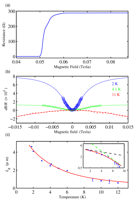
Measurements of the wire’s resistance were performed using a bridge circuit similar to that of Ref.Chandrasekhar : a three terminal arrangement was used here as one of the four original leads was unintentionally blown out as the sample cooled to 4.2 K. One side of the sample was connected to the bridge and the voltage probe through separate leads, while the other side of the sample was connected to ground and the bridge through the same lead. The sample resistance was distinguished from the lead resistance by measuring the resistance of the sample as it transitioned from the superconducting to the normal state as the magnetic field was swept at a temperature below the wire’s transition temperature $T_{c}.$ A measurement of this transition is shown in Fig. 1a.

The diffusion constant $D$ was then calculated using the Einstein relation ($\rho^{-1}=e^{2}gD$), with $e$ being the electron charge and $g$ the electron density of states per unit volume at the Fermi level for aluminumAshcroft . The resistance was measured to be 288 $\mathrm{\Omega}$. Based on the film dimensions, we infer a resistivity $\rho=1.36\times 10^{-8}\pm 0.1\>\mathrm{\Omega m}$. This corresponds to a diffusion constant $D_{\rho}=0.02\pm 0.0015\>\mathrm{m^{2}/s}$. We label $D_{\rho}$ the diffusion constant extracted from this measurement of $\rho$.

We also performed magnetoresistance measurements on the same wire at temperatures above $T_{c}$ in order to extract $L_{\phi}$ and $L_{SO}$. The magnetoresistance in the aluminum wire has contributions from weak localization as well as Maki-Thompson superconducting fluctuations. The analytical form for the weak-localization correction to the resistance of a 1-D wire in a magnetic field is given by

$$\frac{dR^{WL}}{R}=\frac{R(B)-R(B=0)}{R(B=0)}=\frac{3}{2}f_{1}\left(B,b(L_{2})\right)-\frac{1}{2}f_{1}\left(B,b(L_{\phi})\right)$$ (1)

where $1/L_{2}^{2}=1/L_{\phi}^{2}+4/3L_{SO}^{2}$, $L_{\phi}$ is the electron phase coherence and $L_{SO}$ is the spin-orbit coupling length. The functions $f_{1}(B,B1)$ and $b(l)$ are defined in Ref.Ania_Science . The Maki-Thompson contibrution is given by

$$\frac{dR^{MT}}{R}=-\beta\left(\frac{T}{T_{c}}\right)f_{1}\left(B,b(L_{\phi})\right)$$ (2)

where $\beta(t)$ is a function that diverges logarithmically when $t\rightarrow 1$ (see Ref.Ania_Science and references therein). Equation 2 is only valid provided

$$B\ll\frac{k_{B}T}{4De}\ln\left(T/T_{c}\right).$$ (3)

Fits were done using the sum of both equations 1 and 2:

$$\frac{dR}{R}=\frac{dR^{WL}}{R}+\frac{dR^{MT}}{R}$$ (4)

Magnetoresistance measurements were made at a series of temperatures above $T_{c}$ between 1.8 and 12 K. $L_{SO}$ was obtained from fits of the magnetoresistance to Eq. 4 measured at the highest temperatures ($T=9-12\>\mathrm{K}$), where $L_{SO}$ was measured to be $1.54\pm 0.06\>\mathrm{\mu m}$. For fits of the lower temperature data, $L_{SO}$ was fixed at this value, so $L_{\phi}$ was the only fitting parameter. Fits to the magnetoresistace data using Eq. 4 are shown in Fig. 1b. The constraint set by Eq. 3 upon the validity of Eq. 2 sets the limit over which the fits were performed.

Figure 1: (a) Resistance measurement of the aluminum wire as the magnetic field is swept through the critical field $B_{c}$ at a temperature $T=300\,\mathrm{mK}$. The measured resistance in the normal state was 288 $\mathrm{\Omega}$. Due to the loss of one the leads, in series with the sample, we measured a lead resistance of 22 $\mathrm{\Omega}$. This finite resistance is observed even when at $|B|<B_{c}$ and $T<T_{c}$, and it has been subtracted from the trace. (b) Magnetoresistance data for $T=2\;\mathrm{K}\>(\circ)$, $4.1\;\mathrm{K}\>(\times)$ and $11\;\mathrm{K}\>(.)$ and fits (solid lines). The trace for $\mathrm{11\>K}$ has been multiplied by 20. At low temperatures, superconducting fluctuations are the dominant effect observed in the magnetoresistance measurements. The weak localization becomes the dominant effect at $T>8\>\mathrm{K}$. (c) Phase coherence length $L_{\phi}$ extracted from fitting the magnetoresistance data as a function of temperature (points) and fit (solid line) to the expected coherence length assuming both electron-electron and electron-phonon contributions. Inset: Log plot showing $\tau_{e-p}$ and $\tau_{ee}$ contribution as dashed-green and dashed-black lines respectively.

The temperature dependence of $L_{\phi}$ can be explained based on the different contributions to the inelastic collisions of the electrons. Theory predicts that $\tau_{\phi}$ is limited by inelastic collisions with other electrons through the screened Coulomb interactions ($\tau_{ee}$), with phonons ($\tau_{ep}$) and with extrinsic sources such as magnetic impurites. The latter should be negligible for the high purity aluminum source used and since no magnetic impurity has been observed to behave as a localized moment when dissolved in aluminumAshcroft . The fitted values of $L_{\phi}$ as a function of temperature are shown in Fig. 1c. The function used to fit to the data is $L_{\phi}=\sqrt{D\tau_{\phi}}$, where

$$\tau_{\phi}^{-1}=A_{ep}T^{3}+A_{ee}T^{2/3}.$$ (5)

$A_{ep}$ and $A_{ee}$ are fit parameters. The first term of Eq. 5 corresponds to the electron-phonon scattering rate, $\tau_{ep}^{-1}=A_{ep}T^{3}$. From our fit we find that $A_{ep}=2.0\pm 0.2\times 10^{7}\mathrm{s^{-1}K^{-3}}$ which is within a factor of two of previoulsly measured electron-phonon coefficients for comparable Aluminum wiresAnia_Science , Santhanam .

The second term of Eq. 5 corresponds to electron-electron scattering. The wire (and rings) studied here had a width and thickness smaller than $L_{\phi}$. Therefore, the quasi-1D prediction for electron-electron interaction applies and the expression for $\tau_{ee}$ according to Ref.Birge is

$$\tau_{ee}^{-1}=A_{ee}T^{2/3}=\left[\frac{R_{\square}e^{2}k_{B}\sqrt{D}}{2\sqrt{2}\hbar^{2}w}\right]^{2/3}T^{2/3}.$$ (6)

The fitted valued for $A_{ee}$ is $0.65\pm 0.03\times 10^{9}\mathrm{s^{-1}K^{-2/3}}$. The expected theoretical value based on Eq. 6 and a diffusion constant of $D=0.020\>\mathrm{m^{2}/s}$ is $A_{ee}=0.15\times 10^{9}\mathrm{s^{-1}K^{-2/3}}$. Although there is a large discrepancy betwen the expected and fitted value of $A_{ee}$, the primary purpose of these transport measurements is to show that $L_{\phi}$ is greater than the circumference of the rings $L=1.8$ and 2.8 $\mathrm{\mu m}$; therefore we did not look further into this disagreement.

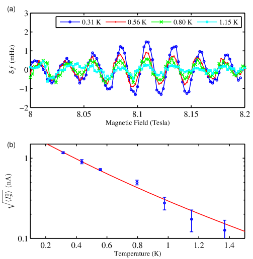
The value for the diffusion constant extracted from the resistivity measurement can then be compared with the diffusion constant extracted from the persistent current measurement (Fig. 2). Using a similar analysis to that explained in Ref. Ginossar2010 we extract a value of $D_{PC}=0.021\pm 0.002\>\mathrm{m^{2}/s}$. We label this value as $D_{PC}$ to distinguish from $D_{\rho}$. $D_{PC}$ and $D_{\rho}$ differ by about $5\%$. This seems reasonable given differences between wire cross section and ring cross section plus statistical uncertainty in $D_{PC}$.

Figure 2: (a) Frequency shift versus magnetic field for a ring of radius $r=296$ nm at different temperatures. The amplitude of frequency oscillations decreases with increasing temperature as expected. The amplitude of the frequency oscillations is converterted into current oscillations amplitude and plotted as a function of temperature in (b). Data (circles) and a fit (solid line) based on analysis similar to that explained in Ref.Ginossar2010 are plotted. From the fit we estimate a diffusion constant of $D=0.021\pm 0.02$.

2 Data Analysis

We inferred the persistent current in each ring by measuring the resonance frequency of the cantilever into which the ring was integrated by driving the cantilever in a phase-locked loopAlbrecht . The method used to infer the current is explained in the supplementary information of Ref.Ania_Science . Here we briefly review this analysis.

As it was shown in Ref.Ginossar2010 , the presence of magnetic field $B_{m}$ inside the metal of the ring leads to an aperiodic modulation of the persistent current oscillations and a change in the flux dependence of of the persistent current from the simpler case where there is only a pure Aharonov-Bohm flux $\phi$ threading the ring. This change is the modification of the time-reversal relation from $I(\phi)=-I(-\phi)$ to $I(B_{m},\phi)=-I(-B_{m},-\phi)$ . As a result, the current is no longer odd in the Aharonov-Bohm flux $\phi$ and it takes the more general form at fixed $B_{m}$

$$I(\phi)=\sum_{p}I_{h/pe}^{+}\sin(2\pi p\frac{\phi}{\Phi_{0}})+I_{h/pe}^{-}\cos(2\pi p\frac{\phi}{\Phi_{0}})$$ (7)

where the variables $I_{h/pe}^{+}$ and $I_{h/pe}^{-}$ are stochastic variables that vary with the magnetic field $B_{m}$ as well as with microscopic disorder, and $\Phi_{0}=h/e$ is a flux quantum. Determining the distribution of $I_{h/pe}^{+}$ and $I_{h/pe}^{-}$ is the central point of the main paper.

We monitor the the cantilever frequency as we vary the magnetic field. The cantilever’s deflection leads to a rotation of the sample, responsible for the coupling between the persistent current and the cantilever. When $\theta\neq\pi/2$ (where $\theta$ is the angle between the plane of the ring and the applied magnetic field $B$), the frequency change is dominated by the following term:

$$\delta f = -\frac{ABf_{0}\gamma_{m}}{kLx_{\mathrm{tip}}}\cos(\theta)\sum_{p}J_{1}\left(2\pi p\frac{AB\cos(\theta)}{\Phi_{0}}\frac{\gamma_{m}x_{\mathrm{tip}}}{L}\right)\times$$

$$\left(I_{h/pe}^{+}\cos(2\pi p\frac{BA\sin\theta}{\Phi_{0}})-I_{h/pe}^{-}\sin(2\pi p\frac{BA\sin\theta}{\Phi_{0}})\right)$$

where $A$ is the area of the ring, $f_{0}$ is the natural resonance frequency of the cantilever, $\gamma_{m}$ is the ratio between the slope of the cantilever and the factor $x_{\mathrm{tip}}/L$ for the flexural mode $m$. For $m=\{1,2\}$, $\gamma_{m}=\{1.377,4.788\}$. $k$ is the cantilever spring constant, $L$ is the length of the cantilever, $x_{\mathrm{tip}}$ is the amplitude of oscillation at the tip of the cantilever, and $J_{1}(x)$ is the first Bessel function of the first kind.

At the temperatures of our experiment the current is dominated by the first harmonic, $p=1$. Thus, for the analysis of the data shown in the main paper we use what in the supplementary online information (SOI) of Ref.Ania_Science is refered to as method B: we assume that the signal only has the $p=1$ component in Eq. 2 and that the argument of the Bessel function varies only weakly over a given data set. In that case, the change in frequency is essentially the derivative of the persistent current (again ignoring all terms for $p>1$).

$$\frac{\partial I}{\partial B}\thickapprox-\delta f\frac{2\pi A\sin\theta}{\Phi_{0}}\left[\frac{AB\nu\gamma_{m}}{kLx_{\mathrm{tip}}}\cos(\theta)J_{1}\left(2\pi p\frac{AB\cos(\theta)}{\Phi_{0}}\frac{\gamma_{m}x_{\mathrm{tip}}}{L}\right)\right]^{-1}$$

In order to estimate the current this quantity can be numerically integrated. However, since we are interested in the statisitics of the variables $I_{h/e}^{\pm}$, we perform the analysis on $I^{\prime}$defined as

$$I^{\prime}(B)=\frac{\Phi_{0}}{2\pi A\sin\theta}\frac{\partial I}{\partial B}$$ (9)

The normalization is such that the oscillations of $I^{\prime}(B)$ have the same amplitude as those in $I(B)$. The reason we use $I^{\prime}$ is that the numerical integration can introduce unwanted correlations in the values of the variables $I_{h/e}^{\pm}$.

2.1 Drift removal

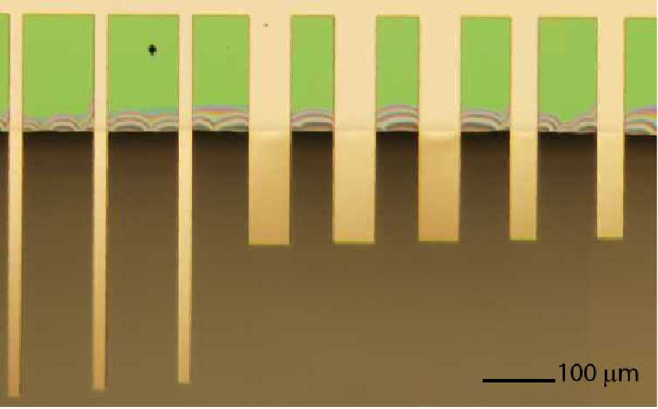
We measured cantilevers similar to the ones shown in Fig. 3. We fabricated long $(l\sim 400\>\mathrm{\mu m})$ and short $(l\sim 100\>\mathrm{\mu m})$ cantilevers, with three different widths ($w=20$, 40 and 60 $\mathrm{\mu m}$). The signal $\delta f$ was larger for the shortest cantilevers. However, their noise peformance was very poor, presenting frequency noise with a power dependence $\sim 1/f^{n}$ with $n\approx 2$, preventing our measurements from achieving the thermal noise limit. However, for the long cantilevers the noise performance of the frequency measurement did reach the thermal noise limit (see Sect. 2.2.1).

Figure 3: Optical micrograph of cantilevers similar to those used for the measurement of persistent current in the main text. The ring sample on each cantilever is not visible.

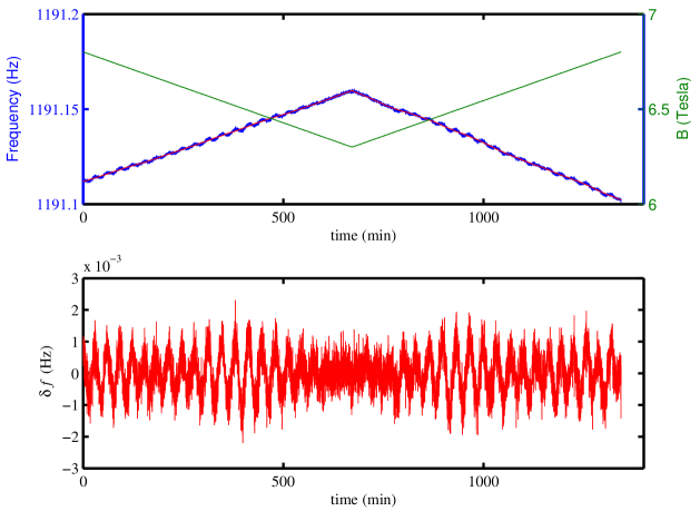
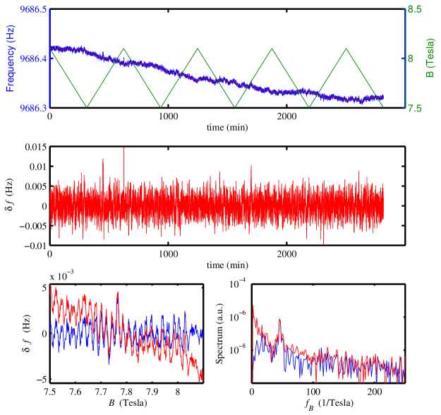
Raw data of the frequency measurements of two kind of cantilevers are shown in figures 4 and 5. In both figures we can see a drift in the cantilever’s resonance frequency with time, but with very different characterisitics. In Fig. 4 the Aharonov-Bohm (AB) oscillations can be easily distinguished on top of a mostly magnetic-field dependent drift. This drift is removed using MATLAB’s local regression algorithm for the LOWESS (Locally Weighted Scatterplot Smoothing) routine with a first degree polynomial. We have observed that if we choose the window of the LOWESS routine to be the equivalent of 5 AB oscillations, the peak of our signal in its Fourier transform is unchanged by the drift removal process.

For a thermally limited frequency measurement, shorter cantilevers should have a greater signal-to-noise ratio, but we found that, in practice, their frequency noise was significantly worse than the longer cantilevers. Thus, for shorter cantilevers, the frequency measurements were not thermally limited. This is obvious in figures 5a and b where it is not possible to discern the AB oscillations at first sight. In Fig. 5c and d we show the averaged data and their spectral densities with and without LOWESS drift removal in order to show that our procedure does not convert a noise shoulder into a peak.

Figure 4: (a) Cantilever frequency (blue left axis) as a function of time as the magnetic field (green right axis) is varied for sample 6. On top of a magnetic-field-dependent background, the oscillations due to the persistent current are obvious and the drift in the cantilever frequency is easily removed by using local regression. After substracting the drift calculated using LOWESS (red trace) we obtain the oscillations shown in (b).

Figure 5: (a) Cantilever frequency (blue left axis) as the magnetic field (green right axis) is varied for sample 2. In this case, the time dependent background is so large, it is hard to distinguish the AB oscillations even after removing the drift as shown in (b). (c) The AB oscillations can be easily distinguished after averaging all the data with the drift (red) and with the drift substracted (blue). This proves that the observed oscillations are not an artifact of the procedure used to remove the drift. (d) Spectral density of (c) showing that the procedure used to remove the drift does not affect the amplitude of the observed oscillations.

2.2 Hilbert Transform

The Hilbert transform of a function $u(t)$ is defined as:

$$\textrm{p.v.}\,\frac{1}{\pi t}\otimes u(t)=H[u(t)]\equiv\hat{u}(t)$$

where p.v. is the Cauchy principal value and $\otimes$ indicates convolution. The Bedrosian theorem states that the Hilbert transform acting on the product of two functions $x(t)=A(t)\times h(t)$ can be written as

$$H[A(t)h(t)]=A(t)H[h(t)]$$ (10)

if the Fourier spectra for $A(t)$ and $h(t)$ are disjoint in frequency space and if the spectrum for $h(t)$ is concentrated at higher frequencies than those of $A(t)$. For example, if $h(t)$ is a periodic function $h(t)=\cos\phi(t)$, $\hat{h}(t)=\sin\phi(t)$. In this regime, then the following relations hold Huang :

$$x(t)=A(t)\cos\phi(t)$$ (11)

$$A(t)=\textrm{abs}(x(t)+i\hat{x}(t))$$ (12)

$$\phi(t)=\textrm{arg}(x(t)+i\hat{x}(t))$$ (13)

For the work described in this paper, the Hilbert transform is used to analyze two separate data sets. In the first case, the Hilbert transform is applied to raw interferometer data (i.e. cantilever position vs. time). This technique allows us to generate densely sampled frequency vs. time traces, which are used to diagnose the sources of noise in the measurement. We discuss this technique in section 2.2.1. In the second case, the Hilbert transform is used to extract the persistent current quadrature amplitudes $I_{h/e}^{\pm}$ from the persistent current data. This is discussed in section 2.2.2.

2.2.1 Phase Noise Analysis

As explained in Ref.Ania_Science , the persistent current measurement is at its core a frequency ($f$) measurement of a driven cantilever. In order to better understand the specific noise sources of the measurement system, it is beneficial to have access to the noise spectral density $S_{f}(\omega)$ of raw frequency data $f(t)$

$$S_{f}(\omega)=2\lim_{T\rightarrow\infty}\frac{\left|F_{T}(\omega)\right|^{2}}{T}$$

where $F_{T}(\omega)$ is the windowed fourier transform of $f(t)$

$$F_{T}(\omega)=\intop_{-T/2}^{T/2}dt^{\prime}f(t)e^{i\omega t^{\prime}}$$

The factor of 2 comes from the fact that we are only considering single-sided spectral densities (thus we only consider $\omega>0$ values). For the work described in the main text, we utitlize a technique involving the Hilbert transform to measure the frequency $f(t)$. The Hilbert transform is applied to cantilever position data obtained by an optical-fiber interferometer.

If the interferometer data contains more than one frequency component, we can define an “instantaneous frequency” $f(t)=f_{0}+f_{noise}(t)$. Here $f_{noise}(t)$ is a stochastic variable with zero mean and $f_{0}$ is a constant. We will consider the limit in which the Fourier transform of the cantilever position is sharply peaked at $f_{0}$ and also $f_{0}\gg\Delta f$, where $f_{0}$ is the center frequency and $\Delta f$ is the width of the peak. In this limit, the Bedrosian theorem (Eq. 10) holds, and we can use the Hilbert transform to calculate the cantilever phase vs. time with Eq. 13.

We convert the phase versus time $\phi(t)$ of the cantilever’s motion to an instantaneous frequency $f(t)$ via the relationship:

$$2\pi f(t)=\frac{d\phi}{dt}$$ (14)

The frequency noise spectrum is related to the phase noise spectrum by $S_{f}=(\omega/2\pi)^{2}S_{\phi}$ by Eq. (14). We can then compare the measured $S_{f}$ to theoretical predictions for the frequency noise of a driven limit-cycle oscillator subject to a white force noise and a white displacement noise in the detection Albrecht

$$S_{f,\,\mathrm{thermal}}(\omega) = \frac{f_{0}k_{B}T}{\pi kQx_{\mathrm{tip}}^{2}}$$

$$S_{f,\,\mathrm{detector}}(\omega) = \frac{2S_{x}^{\mathrm{imp}}}{x_{\mathrm{tip}}^{2}}\left(\frac{\omega}{2\pi}\right)^{2}$$ (15)

where $k$ is the resonator spring constant, $Q$ is the resonator quality factor, $x_{\mathrm{tip}}$ is the resonator displacement amplitude, and $S_{x}^{\mathrm{imp}}$ is the displacement noise of the detector. The imprecision $S_{x}^{\mathrm{imp}}$ in the measurement of the cantilever’s motion arises from fluctuations both in the laser used to monitor the cantilever and in the detector used to measure the laser signal. The dominant noise source in our case is the electronic noise from the photoreciver. In order to convert the voltage at the output of the photodetector into cantilever motion, we measure this voltage when the cantilever is only excited by a thermal force. The magnitude of the cantilever’s thermal motion can be computed from the equipartition theorem which states that at thermal equilibrium

$$k\left\langle x^{2}\right\rangle=k_{B}T$$ (16)

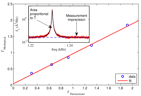
The spectrum of the voltage $S_{V}$ at the output of the photodectector has the shape of lorentzian curve on top of an offset (inset of Figure 6). This offset consists of the measurement imprecision $S_{x}^{\mathrm{imp}}$. By measuring $S_{V}$ at different temperatures (Figure 6), we can properly convert the volts at the output of the detector into displacement of the cantilever and calculate the imprecision $S_{x}^{\mathrm{imp}}$ of our detector.

Figure 6: Thermal motion of the cantilever in units of temperature (Eq. 16) as a function of the fridge temperature. This motion is measured as a voltage at the output of the photodetector and converted into displacement units (inset). The spectral density of the voltage has two constributions: a white background that consists of the measurement imprecision $S_{x}^{\mathrm{imp}}$ coming from the voltage noise of our photodetector (dashed blue line in the inset) , and a lorentzian curve that consists of the thermal motion of the cantilever. Measuring the detector’s voltage fluctuations at different temperatures allows us to calibrate the intereferometer response.

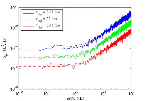
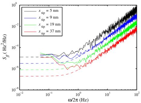
In these measurements, for some cantilevers, we notice a strong deviation from the prediction at low frequencies. This low-frequency behavior seems to correlate with the amount of mechanical nonlinearity in the cantilever (determined, e.g., by a non-Lorentzian resonance for large $x_{\mathrm{tip}}$). For samples 3-8, there was very little nonlinearity and the frequency noise behaves as expected (Fig. 7). For samples 1 and 2, we noticed a large amount of mechanical nonlinearity and also a large amount of low-frequency noise (Fig. 8).

Figure 7: Frequency noise for sample 4. The solid lines represent the frequency noise spectrum data obtained using the Hilbert transform technique described above at various oscillator drive strengths. The dashed lines are the theoretical noise curves calculated with Eq. 15 (no fit parameters). There are two major contributions to the noise: thermal fluctuations driving the cantilever, and the intrinsic detector noise. The detector noise was extracted from the actual interferometer noise. For this cantilever, $Q=5700$, $T=320\>\mathrm{mK}$, $f_{0}=966\>\mathrm{Hz}$ and $k_{L}=4.0\times 10^{-5}\>\mathrm{N/m}.$

Figure 8: Frequency noise for sample 2. The solid lines represent the frequency noise spectrum data obtained using the Hilbert transform technique described above at various oscillator drive strengths. The dashed lines are the theoretical noise curves calculated with Eq. 15 (no fit parameters). This sample exhibited strongly nonlinear behavior and its low-frequency noise deviates from the theoretical curves. For this cantilever, $Q=35000$, $T=320\>\mathrm{mK}$, $f_{0}=11827\>\mathrm{Hz}$ and $k_{L}=1.7\times 10^{-3}\>\mathrm{N/m}.$

2.2.2 Calculating the Persistent Current Amplitude

The goal of the work in the main text is to measure the statistics of the quadrature amplitudes of the AB oscillations $I_{h/e}^{\pm}$. This amplitude slowly changes due to the magnetic field that penetrates the metal of the ring Ginossar2010 . Since our data is dominated by the first harmonic of Eq. 7 (no higher harmonics are visible in the data) the normalized derivative of the current $I^{\prime}$ (Eq. 9) takes the form:

$$I^{\prime}(B) = I_{h/e}^{+}\cos(2\pi p\frac{\phi}{\Phi_{0}})-I_{h/e}^{-}\sin(2\pi p\frac{\phi}{\Phi_{0}})$$ (17)

$$= I_{h/e}(B)\cos\left(2\pi p\frac{BA\sin\theta}{\Phi_{0}}+\alpha(B)\right)$$ (18)

where $I_{h/e}(B)$ is the amplitude of the current and $\cos\left(2\pi p\frac{BA\sin\theta}{\Phi_{0}}-\alpha(B)\right)$ represents the AB oscillations.

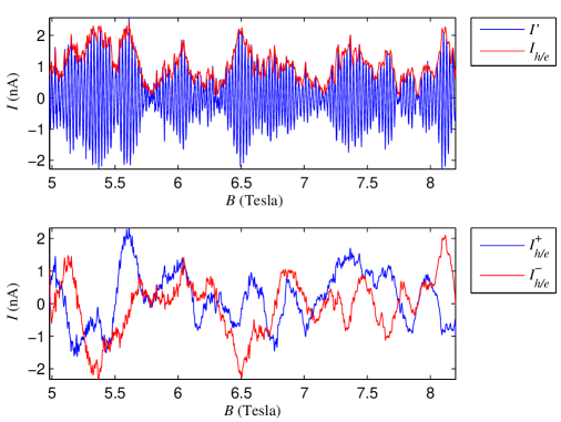
The correlation field $B_{c}$ sets the field scale over which $I_{h/e}(B)$ changes. In the limit that $B_{c}$ is “large enough” ($B_{c}\gg\Phi_{0}/A$), $I_{h/e}(B)$ is a slowly-varying function compared to $\cos(2\pi p\frac{BA\sin\theta}{\Phi_{0}}-\alpha)$ and the Bedrosian theorem (10) holds. The AB frequency is also sharply peaked in Fourier space, with a well-defined frequency given by the dimensions of the ring. Thus, comparing (12) and (17), we can obtain $I_{h/e}(B)$ and $\alpha$ using the Hilbert transform. This also allows us to determine the quadrature variables $I_{h/e}^{+}=I_{h/e}\cos(\alpha)$ and $I_{h/e}^{-}=I_{h/e}\sin(\alpha)$. This technique is illustrated in Fig. 9.

Figure 9: (a) Hilbert transform for the data from sample 6. From this trace we obtain $I_{h/e}(B)$ and $\alpha$ (not shown). (b) Using the data from (a) we can infer the values for $I_{h/e}^{+}$ and $I_{h/e}^{-}$.

2.3 Definition of the cumulants and statistical moments

For the purpose of this manuscript, it is convenient to have a consistent definition of the various moments and cumulants. The raw moments $\mu^{\prime}_{r}$ and central moments $\mu{}_{r}$ of a stochastic variable $x$ are defined as

$$\mu^{\prime}_{r} = \left\langle x^{r}\right\rangle$$ (19)

$$\mu{}_{r} = \left\langle\left(x-\mu^{\prime}_{1}\right)^{r}\right\rangle$$

The cumulants $\left\langle\left\langle I^{n}\right\rangle\right\rangle$ are most easily defined in terms of the central moments:

$$\left\langle\left\langle I^{2}\right\rangle\right\rangle = \mu_{2}$$

$$\left\langle\left\langle I^{3}\right\rangle\right\rangle = \mu_{3}$$

$$\left\langle\left\langle I^{4}\right\rangle\right\rangle = \mu_{4}-3\mu_{2}^{2}$$ (20)

$$\left\langle\left\langle I^{5}\right\rangle\right\rangle = \mu_{5}-10\mu_{3}\mu_{2}$$

$$\left\langle\left\langle I^{6}\right\rangle\right\rangle = \mu_{2}-15\mu_{4}\mu_{2}-10\mu_{3}^{2}+30\mu_{2}^{3}$$

2.4 Finite sample statistics

In Ref.Ginossar2010 it was mentioned that in the presence of an additional large in-plane magnetic field $B_{m}$ penetrating the metal ring, the effective disorder of the ring changes, implying that averaging over magnetic field is equivalent to an ensemble averageLee1985a . However, our finite magnetic field range means that in practice, we have a finite number of realizations from this ensemble. In order to estimate the statistical uncertainty in our estimates of the cumulants due to this finite sample size, we use the results of Ref.ErgodicityProblem .

The statistical uncertainty of the cumulants ($\left\langle\left\langle I^{n}\right\rangle\right\rangle$) due to a finite sample size can be expressed in terms of the normalized correlation function $C(x)$ defined as

$$C\left(\frac{B-B^{\prime}}{B_{c}}\right) = \frac{\left\langle I(B)I(B^{\prime})\right\rangle}{\left\langle I^{2}\right\rangle}$$

where $C$ decays from $C(0)=1$ to $C(\infty)=0$, and $B_{c}$ is the correlation field, which sets a rough order of magnitude over which the persistent current is correlated. Expressions for $C$ are provided in Ref.Ginossar2010 . The typical value of a cumulant calculated from a finite ensemble is given by

$$\left\langle\left\langle\left\langle I^{n}\right\rangle\right\rangle^{2}\right\rangle_{B} = \left\langle\left\langle I^{n}\right\rangle\right\rangle^{2}+a_{n}\frac{B_{c}}{B_{\text{span}}}\left\langle\left\langle I^{2}\right\rangle\right\rangle^{n}$$

where $a_{n}=n!\int_{-\infty}^{\infty}[C(x)]^{n}dx$, and $B_{\text{span}}$ is the total magnetic field range over which data is taken. The theoretical prediction for the higher order cumulants of the persistent current quadratures is

$$\left\langle\left\langle I^{n}\right\rangle\right\rangle\sim\frac{I_{\mathrm{typ}}^{n}}{g^{n-2}}$$

for $n>2$, where the typical current is defined as $I_{\mathrm{typ}}=\sqrt{\left\langle I^{2}\right\rangle}$Houzet2010 . In our case $g\sim 10^{4}$ and thus we expect a gaussian distribution for $I_{h/e}^{\pm}$ and the statistical error is thus given by

$$\delta\left\langle\left\langle I^{n}\right\rangle\right\rangle=\sqrt{a_{n}\frac{B_{c}}{B_{\text{span}}}\left\langle I^{2}\right\rangle^{n}}$$ (21)

For an estimate of this term, we can consider the case for a spinless electron at $T=0$ and large $B_{m}$ (so that we can ignore the Cooperon contribution) and only include the first harmonic of the PC. In this case

$$C(x)=\left(1+|x|+\frac{x^{2}}{3}\right)e^{-|x|}$$ (22)

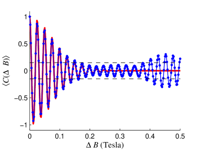
For this simplified case, the first 4 coefficients are $a_{2}=7$, $a_{3}=16.61$, $a_{4}=56.48$, and $a_{5}=249.55$. Experimental values of the cumulants of the persistent currents are considered sound only if they comfortably exceed the systematic error $\sqrt{a_{n}\frac{B_{c}}{B_{\text{span}}}\left\langle I^{2}\right\rangle^{n}}$ (Eq. 21). The actual correlation function for our case is more complicated than Eq. 22 and is a function of $T$ and $L_{SO}$. It can be numerically implemented using Ref.Ginossar2010 . A fit to the correlation function $C(B/B_{c},T,L_{SO})$ of our data is shown in Fig. 10.

We can also define an effective number of samples based on the expected statistical uncertainty for the cumulants of an ensemble of $N_{\text{eff}}$ samples kendall :

$$\delta\left\langle\left\langle I^{n}\right\rangle\right\rangle=\sqrt{\frac{n!\left\langle\left\langle I^{2}\right\rangle\right\rangle^{n}}{N_{\text{eff}}}}.$$

By comparing the latter with Eq. 21, we can then define $N_{\text{eff}}$ as

$$N_{\text{\text{n,eff}}}=\frac{n!B_{\text{span}}}{a_{n}B_{c}}.$$ (23)

Figure 10: Persistent current autocorrelation for sample 6. Blue represents the autocorrelation of the data shown in Fig. 20 and red is the fit using Ref.Ginossar2010 . The estimated correlation field in this case is $B_{c}=32\>\mathrm{mT}.$ In order to estimate the standard error in the autocorrelation (dashed horizontal lines), we assume that this is approximatly given by the standard error for the correlation coefficient $1/\sqrt{N_{\text{{{eff}}}}}\approx 0.15$. As it can be seen in the figure, fluctuations of this order are present at large $\Delta B\gg B_{c}$, where the autocorrelation of an infinitely large data set would be expected to vanish.

2.5 Finite signal to noise

Another source of error in our estimate of the cumulants is the finite sensitivity of our setup. In order to estimate this error, we have to calcualte the appropriate expression for error propagation in our analysis. Our case is somewhat confusing, since $x_{i}$ itself is an stochastic variable, so really we have $x_{i,meas}=x_{i}+\delta x_{i}$. First let’s consider the general equation for the error propagation for a general function $f(x_{1},x_{2}...,x_{N})$. If $x_{i}$ is known only to within an error $\delta x_{i}$ then the error in $f$ is given by

$$\delta^{2}f=\sum_{i}\left(\frac{\partial f}{\partial x_{i}}\delta x_{i}\right)^{2}$$ (24)

Let’s first consider the case of the central moment as cumulants are easily definined in terms of them:

$$f(x_{i})=\mu_{r}=\frac{1}{N}\sum_{i}\left(x_{i}-\mu^{\prime}_{1}\right)^{r}$$

Then

$$\left\langle\delta^{2}\mu_{r}\right\rangle = \left(\frac{r}{N}\right)^{2}\sum_{i}\left(x_{i}-\mu^{\prime}_{1}\right)^{2r-2}\left\langle\delta^{2}x_{i}\right\rangle$$ (25)

$$= \frac{r^{2}}{N}\mu_{2r-2}\left\langle\delta^{2}x\right\rangle$$

There are two assumptions used for Eq. 25. First, we assume that the noise $\delta x_{i}$ from the different magnetic field points (labeled with the index $i$) are uncorrelated. This does not mean that the different $x_{i}$’s are uncorrelated. The second assumption is that $\delta^{2}x_{i}$ can be replaced by an average $\delta^{2}x$. Although not completely accurate, since the sensitivity of our measurement is lower at lower magnetic fields, we did compensate for the loss of sensitivity by averaging longer at low magnetic fields.

The expressions for the second and third cumulants are the same as for the second and third central moments. Thus, Eq. 25 gives their measurement uncertainty. For the forth, fifth and sixth cumulant we can use the following heuristic approachkendall . We start with the definition of the cumulants (Eq. 20), from which the following expressions are derived:

$$\delta\left\langle\left\langle I^{4}\right\rangle\right\rangle = \delta\mu_{4}-6\mu_{2}\delta\mu_{2}$$

$$\delta\left\langle\left\langle I^{5}\right\rangle\right\rangle = \delta\mu_{5}-10\mu_{2}\delta\mu_{3}-10\mu_{3}\delta\mu_{2}$$

$$\delta\left\langle\left\langle I^{6}\right\rangle\right\rangle = \delta\mu_{6}-15\mu_{4}\delta\mu_{2}-15\mu_{2}\delta\mu_{4}-20\mu_{3}\delta\mu_{3}+90\mu_{2}^{2}\delta\mu_{2}$$

Then, for example, for the fourth cumulant:

$$\left\langle\delta^{2}\left\langle\left\langle I^{4}\right\rangle\right\rangle\right\rangle=\delta^{2}\mu_{4}+36\mu_{2}^{2}\delta^{2}\mu_{2}-12\mu_{2}\left\langle\delta\mu_{4}\delta\mu_{2}\right\rangle$$ (26)

The covariance $\left\langle\delta\mu_{4}\delta\mu_{2}\right\rangle$ is not necessarily zero and it can be derived using a similar approach as the one used to derive Eq. 25:

$$\left\langle\delta\mu_{r}\delta\mu_{s}\right\rangle=\frac{rs}{N}\mu_{r+s-2}\left\langle\delta^{2}x\right\rangle$$

Similar expressions to Eq. 26 for $\left\langle\left\langle I^{5}\right\rangle\right\rangle$ and $\left\langle\left\langle I^{6}\right\rangle\right\rangle$ can be derived.

2.6 Data

Following, we show a table with all the estimated cumulants and estimated errors for the cumuluants of all 8 samples. The cumulants of both $I^{+}$ and $I^{-}$ have been combined for each of the rings. In order to account for variations between rings the different cumulants are normalized by the variance $\left\langle\left\langle I^{2}\right\rangle\right\rangle$; thus we define a normalized cumulant $\kappa_{n}\equiv\left\langle\left\langle I^{n}\right\rangle\right\rangle/\left\langle\left\langle I^{2}\right\rangle\right\rangle^{n/2}$.

Sample #	$r$ (nm)	$B_{c}$ (mT)	$N_{\mathrm{2,eff}}$	$\left\langle\left\langle\left(I^{\pm}\right)^{2}\right\rangle\right\rangle(\mathrm{nA^{2}})$	$\kappa_{3}$
1	296	$16\pm 1$	63	$0.46\times(1\pm 0.18\pm 0.02)$	$0.065\pm 0.28\pm 0.05$
2	296	$25\pm 1.5$	43	$0.37\times(1\pm 0.22\pm 0.02)$	$0.23\pm 0.34\pm 0.04$
3	448	$9\pm 1$	55	$0.0031\times(1\pm 0.2\pm 0.03)$	$0.21\pm 0.31\pm 0.08$
4	448	$17\pm 1$	34	$0.0063\times(1\pm 0.24\pm 0.02)$	$-0.25\pm 0.4\pm 0.07$
5	296	$22\pm 1$	56	$0.597\times(1\pm 0.19\pm 0.01)$	$0.18\pm 0.29\pm 0.03$
6	296	$32\pm 2$	44	$0.67\times(1\pm 0.21\pm 0.01)$	$0.001\pm 0.34\pm 0.02$
7	296	$20\pm 1$	81	$0.26\times(1\pm 0.16\pm 0.01)$	$0.083\pm 0.24\pm 0.03$
8	418	$11\pm 1$	36	$0.022\times(1\pm 0.23\pm 0.02)$	$-0.05\pm.37\pm 0.05$

Sample #	$\kappa_{4}$	$\kappa_{5}$	$\kappa_{6}$
1	$-0.052\pm 0.51\pm 0.1$	$-0.12\pm 1.1\pm 0.25$	$-0.91\pm 2.6\pm 0.47$
2	$-0.0271\pm 0.62\pm 0.07$	$-0.83\pm 1.3\pm 0.2$	$-0.93\pm 3.1\pm 0.41$
3	$0.29\pm 0.58\pm 0.18$	$-0.05\pm 1.23\pm 0.5$	$-0.84\pm 2.9\pm 1.13$
4	$0.56\pm 0.75\pm 0.16$	$0.27\pm 1.58\pm 0.5$	$-0.043\pm 3.7\pm 1.32$
5	$-0.25\pm 0.54\pm 0.04$	$-0.17\pm 1.15\pm 0.14$	$0.36\pm 2.7\pm 0.28$
6	$-0.61\pm 0.637\pm 0.03$	$-0.05\pm 1.35\pm 0.09$	$2.23\pm 3.15\pm 0.18$
7	$0.065\pm 0.45\pm 0.07$	$0.51\pm 0.95\pm 0.23$	$2.85\pm 2.23\pm 0.45$
8	$0.2\pm 0.68\pm 0.086$	$0.12\pm 1.4\pm 0.23$	$-2.1\pm 3.35\pm 0.58$

Table 1: Higher order moments of the quadrature amplitudes of the persistent current for all the measured samples. The first error indicates the standard error due to finite-size sample and the other represents uncertainty from noise in the frequency measurement. $N_{2,\text{eff}}$ indicates the effective number of samples for a given ring using Eq. 23 multiplied by 2 as we use both quadratures $I^{\pm}$ to calculate the cumulants.

3 Measurement diagnostics

We performed a set of diagnostic measurements similar to those described in Ref.Ania_Science . Specifically, we measured the effects of the readout laser power on the measured frequency, we compared the extracted current using the two first modes of the cantilever motion and we checked the effects of cantilever oscillation amplitude.

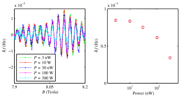
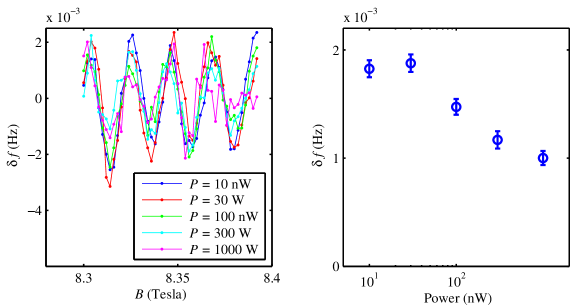
Figures 11 and 12 show the effect of varying the laser power upon the persistent current data measured on two different cantilevers for different incident laser powers. For different cantilevers, we observed two qualitatively different types of dependence upon the laser power. We believe this difference is due to the different widths of the cantilevers. The data of samples 1-4 where taken with an incident power of 10 nW. However, for samples 5-7, the data was taken with an laser incident power of 3 nW as they presented a stronger power dependence. Sample 8 was taken with a laser power of 5 nW in a previous cooldown (Ref.Ania_Science ).

Sample #	$r$ (nm)	$w$ (nm)	$t$ (nm)	$l_{\mathrm{cantilever}}$ ($\mathrm{\mu m})$	$w_{\mathrm{cantilever}}$ ($\mathrm{\mu m})$
1	296	90	115	114	40
2	296	90	115	126	40
3	448	90	115	395	40
4	448	90	115	398	40
5	296	90	115	370	20
6	296	85	115	359	20
7	296	95	115	352	20
8	418	85	90	438	60

Table 2: Sample parameters. All the measurements were done at a 45-degree angle between the cantilever and ring plane and the magnetic field. All the cantilevers had a thickness of 118 nm except for sample 8 which had a thickness of $340\text{ nm}$. Sample 8 was measured in a separate cooldown.

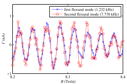
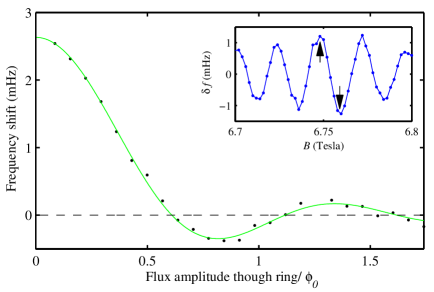
In Fig. 13 we demonstrate that the inferred current is the same whether the cantilever’s first or second flexural mode is used, indicating that persistent current is independent of excitation frequency of the cantilever. Finally, in Fig. 14 we show that the cantilever’s frequency depends upon the amplitude of its motion as would be expected if the persistent current remains in its equilibrium state (Eq. 2). To generate the data shown in Fig. 14, the resonant frequency of cantilever 5 was measured at two different magnetic fields (indicated in the inset figure with two arrows) as a function of cantilever amplitude $x_{\mathrm{tip}}$. Then, the two measured $\delta f$ were substracted in order to remove any kind of amplitude-dependent change in the cantilevers resonance frequency. The cantilever was excited in its first flexural mode.

Figure 11: Left panel: Change in frequency versus magnetic field for a series of laser powers incident on the cantilever. This data was taken with sample 6. The drive was the same for all the traces. Right panel: The mean amplitude of each of the traces from the left panel, plotted versus laser power. For the data of samples 5, 6 and 7 shown in the main paper, $3\text{ nW}$ of laser power was used.

Figure 12: Left panel: Change in frequency versus magnetic field for a series of laser powers incident on the cantilever. This data was taken with sample 2. The drive was the same for all the traces. Right panel: The mean amplitude of each of the traces from the left panel, plotted versus laser power. For the data of samples 1, 2, 3 and 4 shown in the main paper, $10\text{ nW}$ of laser power was used.

Figure 13: The derivative of the persistent current I´ (derived from Eqs. 2 and 9) versus magnetic field measured when oscillating the cantilever at 1.232 kHz (the cantilever’s first flexural resonance) and at 7.77 kHz (the cantilever’s second flexural resonance). The persistent current does not appear to depend on the cantilever oscillation frequency.

Figure 14: Cantilever drive test on sample 5 where we measure the accuracy of Eq. 2. The cantilever amplitude is plotted on the $x$-axis in terms of the amplitude of the flux modulation $\phi_{ac}/\phi_{0}$ through the ring produced by the cantilever motion. Data points reperesent the difference in cantilever frequency shift for the two field values indicated in the inset. The solid curve is a fit using Eq. 2 (with $p=1$) and $r=301\pm 2\,\mathrm{nm}$, consistent with the measured radius and linewidth of our ring (see table 2). Inset: the arrows indicate two field values at which measurements of the cantilever frequency shift were performed as a function of cantilever amplitude.

4 Data of all the samples

4.1 Magnetic field sweeps

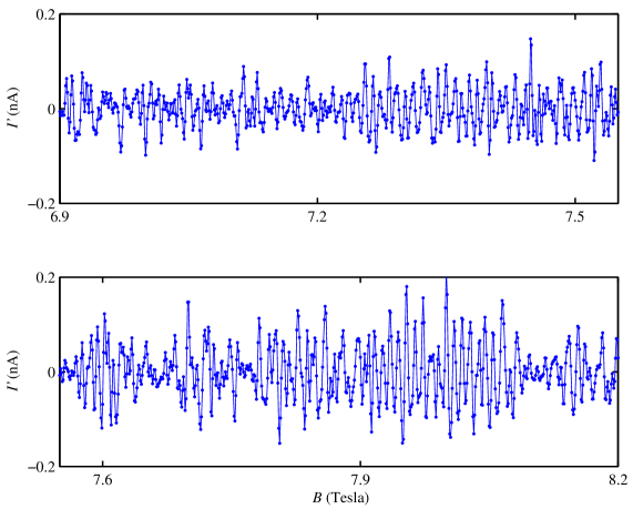
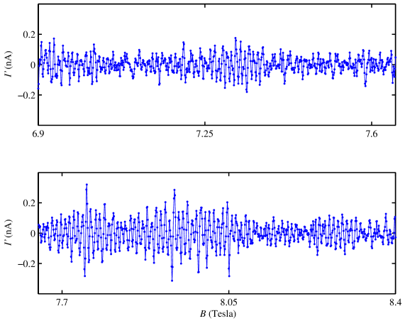
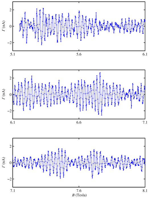
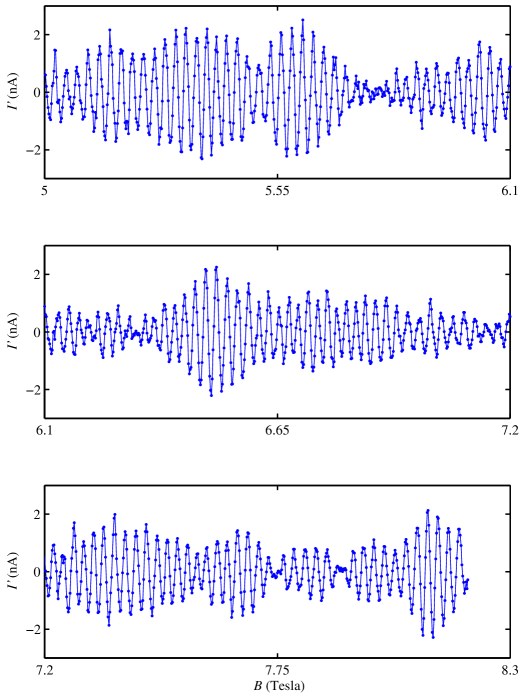
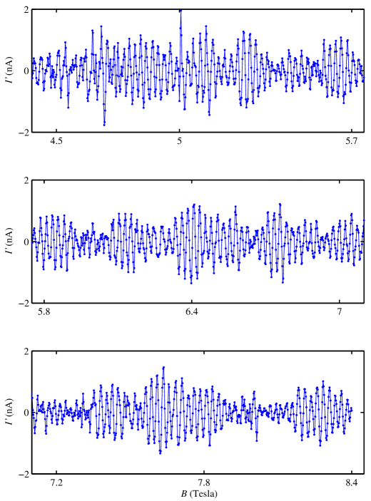
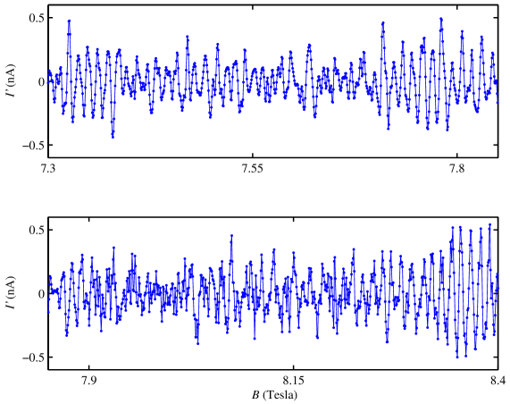
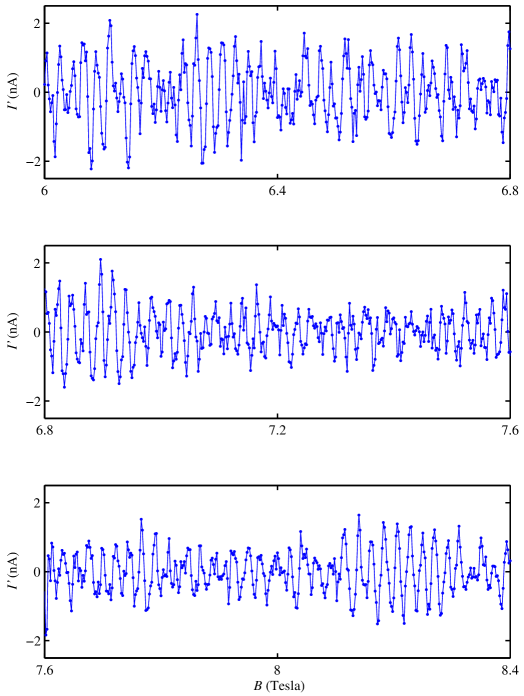
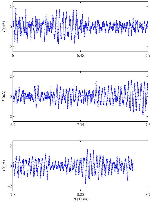
In this last section, we present figures 15-22 where we show the complete $I^{\prime}$ versus magnetic field traces which were analyzed in the main text. These traces were calculated, using method B of Ref.Ania_Science from measurements of the cantilever frequency performed at the refrigerator’s base temperature of 320 mK (365 mK for sample 8).

Figure 15: The derivative of the persistent current $I^{\prime}$ (derived from Eqs. 2 and 9) versus magnetic field for sample 1 at T = 320 mK. The full sweep is separated into three contiguous panels for clarity.

Figure 16: The derivative of the persistent current $I^{\prime}$ (derived from Eqs. 2 and 9) versus magnetic field for sample 2 at T = 320 mK.

Figure 17: The derivative of the persistent current $I^{\prime}$ (derived from Eqs. 2 and 9) versus magnetic field for sample 3 at T = 320 mK.

Figure 18: The derivative of the persistent current $I^{\prime}$ (derived from Eqs. 2 and 9) versus magnetic field for sample 4 at T = 320 mK.

Figure 19: The derivative of the persistent current $I^{\prime}$ (derived from Eqs. 2 and 9) versus magnetic field for sample 5 at T = 320 mK.

Figure 20: The derivative of the persistent current $I^{\prime}$ (derived from Eqs. 2 and 9) versus magnetic field for sample 6 at T = 320 mK.

Figure 21: The derivative of the persistent current $I^{\prime}$ (derived from Eqs. 2 and 9) versus magnetic field for sample 7 at T = 320 mK.

Figure 22: The derivative of the persistent current $I^{\prime}$ (derived from Eqs. 2 and 9) versus magnetic field for sample 8 at T= 365 mK.

References

• [1] Houzet, M. Distribution function of persistent current. Physical Review B 82, 1–4 (2010).
• [2] Bleszynski-Jayich, A. C. et al. Persistent currents in normal metal rings. Science (New York, N.Y.) 326, 272–5 (2009).
• [3] Ginossar, E. et al. Mesoscopic persistent currents in a strong magnetic field. Physical Review B 81, 1–11 (2010).
• [4] Lee, P. A. & Stone, A. D. Universal conductance fluctuations in metals. Physical Review Letters 55, 1622–1625 (1985).
• [5] Tsyplyatyev, O., Aleiner, I., Fal’ko, V. & Lerner, I. Applicability of the ergodicity hypothesis to mesoscopic fluctuations. Physical Review B 68, 17–20 (2003).
• [6] Chandrasekhar, V. Electron Quantum Interference in Small Metal Wires and Loops. Ph.D. thesis, Yale University (1989).
• [7] Ashcroft, N. W. & Mermin, N. D. Solid State Physics (Saunders College Publishing, Fort Worth, 1976).
• [8] Santhanam, P., Wind, S. & Prober, D. E. Localization, superconducting fluctuations, and superconductivity in thin films and narrow wires of aluminum. Physical Review B (1987).
• [9] Pierre, F. & Birge, N. Dephasing by Extremely Dilute Magnetic Impurities Revealed by Aharonov-Bohm Oscillations. Physical Review Letters 89, 1–4 (2002).
• [10] Albrecht, T. R., Grutter, P., Horne, D. & Rugar, D. Frequency modulation detection using high Q cantilevers for enhanced force microscope sensitivity. Journal of Applied Physics 668–673 (1991).
• [11] Huang, N. E. et al. The empirical mode decomposition and the Hilbert spectrum for nonlinear and non-stationary time series analysis. Proceedings of the Royal Society A: Mathematical, Physical and Engineering Sciences 454, 903–995 (1998).
• [12] Stuart, A. & Ord, J. K. Kendall’s Advanced Theory of Statistics (Oxford University Press, New York, 1987), 5th edn.