Computer Model Calibration Using the Ensemble Kalman Filter
Dave Higdon, Statistical Sciences Group, Los Alamos National Laboratory
Matt Pratola, Statistical Sciences Group, Los Alamos National Laboratory
Jim Gattiker, Statistical Sciences Group, Los Alamos National Laboratory
Earl Lawrence, Statistical Sciences Group, Los Alamos National Laboratory
Charles Jackson, University of Texas Institute for Geophysics
Michael Tobis, University of Texas Institute for Geophysics
Salman Habib, High Energy Physics Division, Argonne National Laboratory
Katrin Heitmann, High Energy Physics Division, Argonne National Laboratory
Steve Price, Fluid Dynamics Group, Los Alamos National Laboratory

The ensemble Kalman filter (EnKF) (Evensen, , 2009a) has proven effective in quantifying uncertainty in a number of challenging dynamic, state estimation, or data assimilation, problems such as weather forecasting and ocean modeling. In these problems a high-dimensional state parameter is successively updated based on recurring physical observations, with the aid of a computationally demanding forward model that propagates the state from one time step to the next. More recently, the EnKF has proven effective in history matching in the petroleum engineering community (Evensen, , 2009b; Oliver and Chen, , 2010). Such applications typically involve estimating large numbers of parameters, describing an oil reservoir, using data from production history that accumulate over time. Such history matching problems are especially challenging examples of computer model calibration since they involve a large number of model parameters as well as a computationally demanding forward model. More generally, computer model calibration combines physical observations with a computational model – a computer model – to estimate unknown parameters in the computer model. This paper explores how the EnKF can be used in computer model calibration problems, comparing it to other more common approaches, considering applications in climate and cosmology.
Keywords: computer experiments; model validation; data assimilation; uncertainty quantification; Gaussian process; parameter estimation; Bayesian statistics

1 Introduction

The ensemble Kalman filter (EnKF) has proven effective in quantifying uncertainty in a number of challenging dynamic, state estimation, or data assimilation, problems. Applications include weather forecasting (Houtekamer et al., , 2005), ocean modeling (Evensen, , 2003), storm tracking (Aksoy et al., , 2009), hydrology (Moradkhani et al., , 2005) and wildfire modeling (Mandel et al., , 2004), just to name a few. In these data assimilation problems, a high-dimensional state parameter is successively updated based on recurring physical observations, with the aid of a computationally demanding forward model that propagates the state from one time step to the next. The EnKF iteratively updates an ensemble of state vectors, using a scheme motivated by the standard Kalman filter (Meinhold and Singpurwalla, , 1983; West and Harrison, , 1997), producing an updated ensemble of states that is affected by both the forward model and the physical observations. More recently, the EnKF has proven effective in history matching in the petroleum engineering community (Evensen, , 2009b; Oliver and Chen, , 2010). Such applications typically involve estimating large numbers of parameters, describing an oil reservoir, using data from production history that accumulate over time. Such history matching problems are especially challenging examples of computer model calibration since they involve a large number of model parameters as well as a computationally demanding forward model. Unlike standard data assimilation problems, here focus is on estimation of a static model parameter vector, rather than an evolving state vector.

This paper explores how the EnKF can be used in computer model calibration problems that typically have a collection of model parameters to be constrained using physical observations. We first use a simple 1-d inverse problem to describe standard Bayesian approaches to produce a posterior distribution for the unknown model parameter vector, as well as the resulting model prediction. We then go on to describe how the EnKF can be used to address this basic problem, with examples taken from the literature in climate and cosmology. We end with conclusions summarizing the strengths and weaknesses of using the EnKF for computer model calibration.

1.1 A simple inverse problem

Figure 1: A simple 1-dimensional inverse problem and resulting posterior density.

In order to describe the basic approaches to inverse problems, we first describe a simple, 1-dimensional inverse problem shown in Figure 1. We take $\eta(\cdot)$ to denote the forward model. It requires a single model parameter $\theta$, producing a univariate output $\eta(\theta)$ that is comparable to a physical measurement $y$. Here we take the sampling model for $y$ to be normally distributed about the forward model’s output when the true value of the model parameter is input

$$L(y|\eta(\theta))\propto\exp\{-\mbox{\small$\frac{1}{2}$}\sigma^{-2}_{y}(y-\eta(\theta))^{2}\}$$

where the observation error is assumed known to be $\sigma_{y}=.1$.

After specifying a standard normal prior for the model parameter, with $\pi(\theta)$ denoting the prior density, the posterior density is given by

$$\pi(\theta|y) \propto L(y|\eta(\theta))\times\pi(\theta)$$

$$\propto \exp\{-\mbox{\small$\frac{1}{2}$}\sigma^{-2}_{y}(y-\eta(\theta))^{2}\}\times\exp\{-\mbox{\small$\frac{1}{2}$}\theta^{2}\}.$$

Thus an evaluation of the posterior requires a run of the forward model. While this simple, 1-dimensional density is trivial to evaluate, many inverse problems have to deal with a large model parameter vector (dimensions ranging from $10$ to $10^{8}$) as well as a computationally demanding forward model that may take a long time to evaluate (our experience ranges from seconds to weeks).

1.1.1 Using a Gaussian process emulator

While Markov chain Monte Carlo (MCMC) remains a popular approach for exploring the resulting posterior distribution (Kaipio and Somersalo, , 2004; Tarantola, , 2005), the demands required by the size of the model parameter vector and the computational demands of the forward model have inspired recent research focused on overcoming these hurdles. These research efforts range from response surface approximation of the forward model $\eta(\cdot)$ (Kennedy and O’Hagan, , 2001; Higdon et al., , 2005), to constructing reduced, or simplified forward models (Galbally et al., , 2010; Lieberman et al., , 2010), to polynomial chaos approximations of the prior model (Ghanem and Doostan, , 2006; Marzouk and Najm, , 2009), to exploiting multiple model fidelities (Christen and Fox, , 2005; Efendiev et al., , 2009).

Figure 2: Using a Gaussian process prior for the forward model to reduce the number of model runs necessary for posterior exploration for the simple inverse problem.

Gaussian processes (GPs) are commonly used to emulate the computer model response, producing a probabilistic description of the response at untried parameter settings – see Kennedy and O’Hagan, (2001) or Bayarri et al., (2007) for just a couple of examples. This basic approach is depicted in Figure 2. In this case, a GP prior is used to model the unknown function $\eta(\cdot)$ and a collection of forward model runs $\eta^{\circ}=(\eta(\theta_{1}^{\circ}),\ldots,\eta(\theta_{m}^{\circ}))^{\prime}$, over a collection of input parameter settings $\theta^{\circ}=(\theta_{1}^{\circ},\ldots,\theta_{m}^{\circ})^{\prime}$, are used to infer the forward model response at untried input parameter settings.

Thus the basic fomulation (1.1) is augmented to incorporate this GP prior for the forward model

$$\eta(\cdot)\sim GP(m(\cdot),C(\cdot,\cdot)),$$

where the mean function $m(\cdot)$ may be a constant (Sacks et al., , 1989; Kennedy and O’Hagan, , 2001), or a more complicated regression function (Craig et al., , 2001; Vernon et al., , 2010), and the covariance function $C(\cdot,\cdot)$ is typically of product form, requiring just a single additional parameter for each dimension of the input parameter. For this simple problem, we take the mean and covariance functions as fixed, leading to the posterior form

$$\pi(\theta|y,\eta^{\circ})\propto\exp\{-\mbox{\small$\frac{1}{2}$}(v_{\theta}+\sigma^{2}_{y})^{-1}(y-\mu_{\theta})^{2}\}\times\exp\{-\mbox{\small$\frac{1}{2}$}\theta^{2}\}.$$

Here $\mu_{\theta}$ and $v_{\theta}$ are the mean and variance given by the GP model after conditioning on the forward model runs $\eta^{\circ}$

$$\mu_{\theta} = C(\theta,\theta^{\circ})C(\theta^{\circ},\theta^{\circ})^{-1}(\eta^{\circ}-m(\theta^{\circ}))+m(\theta)$$

$$v_{\theta} = C(\theta,\theta)-C(\theta,\theta^{\circ})C(\theta^{\circ},\theta^{\circ})^{-1}C(\theta^{\circ},\theta),$$

where, for example, $C(\theta^{\circ},\theta^{\circ})$ produces a $m\times m$ matrix whose $ij$ entry is $C(\theta^{\circ}_{i},\theta^{\circ}_{j})$ and $C(\theta,\theta^{\circ})$ produces a $m$-vector whose $j$th element is $C(\theta,\theta^{\circ}_{j})$. See Higdon et al., (2005) for details regarding the posterior specification when the GP (and other) parameters are not taken as fixed, and the input parameter is multivariate.

1.1.2 Using the ensemble Kalman filter

Below we briefly describe two basic variants of the the EnKF for computer model calibration, differing in how they use the ensemble of model runs to approximate, and represent, the resulting posterior distribution. In both cases, an ensemble of draws $\theta^{\circ}$ from the prior distribution of the model parameter are paired with the resulting simulation output to produce an ensemble of $(\theta^{\circ},\eta(\theta^{\circ}))$ pairs, from which the sample covariance is used to produce an approximation to the posterior distribution. Hence we treat the input parameter settings $\theta^{\circ}_{1},\ldots,\theta^{\circ}_{m}$ as $m$ draws from the prior distribution $\pi(\theta)$. Note that even though the distribution of the simulator response $\eta(\theta)$ is completely determined by the distribution for $\theta$, the EnKF uses a joint normal model for $(\theta,\eta(\theta))$ to motivate its calculations.

Next we describe two variants of the EnKF algorithm for computer model calibration. One uses a Gaussian representation of the posterior distribution, the other uses an ensemble representation.

Gaussian representation

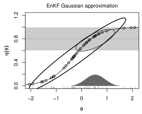
The first approach fits a multivariate normal distribution to the ensemble for $(\theta^{\circ},\eta(\theta^{\circ}))$. The algorithm is depicted in the left frame of Figure 3 and described below.

1. For each of the $m$ simulations form the ensemble of joint vectors

   $$\begin{pmatrix}\theta_{k}^{\circ}\\ \eta(\theta^{\circ}_{k})\end{pmatrix},\,k=1,\ldots,m.$$ (2)

   With these $m$ vectors, compute the sample mean vector $\mu_{\rm pr}$ and sample covariance matrix $\Sigma_{\rm pr}$. For the simple inverse problem here, $\mu_{\rm pr}$ is a $2$-vector and $\Sigma_{\rm pr}$ is $2\times 2$, but this recipe is quite general.

2. In this simple inverse problem, the physical observation $y$ corresponds to the 2nd element of the joint $(\theta,\eta(\theta))$ vector. Take ${H}$ be $(0,1)^{\prime}$ to be the observation matrix. The likelihood can be written

   $$L(y|\eta(\theta))\propto\exp\left\{-\frac{1}{2}\left(y-H\begin{pmatrix}\theta\\ \eta(\theta)\end{pmatrix}\right)^{\prime}\Sigma_{y}^{-1}\left(y-H\begin{pmatrix}\theta\\ \eta(\theta)\end{pmatrix}\right)\right\}.$$ (3)

   More generally the observation operator $H$ can select elements of $\eta(\theta)$ that are observed, or can be specified to interpolate between values of the simulator output.

3. Combining the normal approximation to the prior with the normal likelihood results in an updated, or posterior, distribution for $(\theta,\eta)$ for which

   $$\begin{pmatrix}\theta\\ \eta\end{pmatrix}|y\sim N(\mu_{\rm post},\Sigma_{\rm post}),$$ (4)

   where

   $$\Sigma_{\rm post}^{-1}=\Sigma_{\rm pr}^{-1}+H^{\prime}\Sigma_{y}^{-1}H$$ (5)

   and

   $$\mu_{\rm post}=\Sigma_{\rm post}\left(\Sigma_{\rm pr}^{-1}\mu_{\rm pr}+H^{\prime}\Sigma_{y}^{-1}y\right).$$ (6)

   Note that the posterior mean can be rewritten in a form more commonly used in Kalman filtering

   $$\mu_{\rm post}=\mu_{\rm pr}+\Sigma_{\rm pr}H^{\prime}(H\Sigma_{\rm pr}H^{\prime}+\Sigma_{y})^{-1}(y-H\mu_{\rm pr})$$

   where $\Sigma_{\rm pr}H^{\prime}(H\Sigma_{\rm pr}H^{\prime}+\Sigma_{y})^{-1}$ is the Kalman gain matrix.

The joint normal computations used here effectively assume a linear plus Gaussian noise relationship between $\theta$ and $\eta(\theta)$, inducing a normal posterior for $\theta$.

Figure 3: Left: Gaussian representation of the posterior distribution for $(\theta,\eta(\theta))$ resulting from the ensemble Kalman filter (EnKF). The approximate normal prior distribution for $(\theta,\eta(\theta))$ is depicted by the black ellipse, estimated from the ensemble (circle plotting symbols). The resulting posterior distribution is approximated as normal, depicted by the gray ellipse. The marginal posterior for $\theta$ is given by the shaded density. Right: the ensemble representation of the posterior distribution for $(\theta,\eta(\theta))$ resulting from the EnKF. Here the updated sample (gray dots) are approximate draws from the posterior distribution.

Ensemble representation

The second approach is basically the usual EnKF as applied to time evolving systems, but here, only for a single time step. The goal is to perturb each member of the ensemble $(\theta^{\circ}_{k},\eta(\theta^{\circ}_{k}))$, in order to produce an updated member $(\eta_{k}^{(1)},\theta^{(1)}_{k})$ whose mean and variance match the posterior produced by the Gaussian representation EnKF described above. This updated member is not produced with the simulator so that $\eta^{(1)}_{k}$ will not be equal to the simulator evaluated at updated parameter value $\eta(\theta^{(1)}_{k})$. Here we describe the perturbed data version of the EnKF described in Evensen, (2009b). A number of variants of this basic approach exist; see Anderson, (2001) and Szunyogh et al., (2008), for example. The algorithm is given below.

1. Construct the sample covariance matrix $\Sigma_{\rm pr}$ as in Step 1 of the previous algorithm.

2. For $k=1,\dots,m$ do:

   1. Draw a perturbed data value $y_{k}\sim N(y,\Sigma_{y})$.

   2. Produce the perturbed ensemble member

      $$\begin{pmatrix}\theta^{(1)}_{k}\\ \eta_{k}^{(1)}\end{pmatrix}=\Sigma_{\rm post}\left(\Sigma_{\rm pr}^{-1}\begin{pmatrix}\theta^{\circ}_{k}\cr\eta(\theta^{\circ}_{k})\end{pmatrix}+H^{\prime}\Sigma_{y}^{-1}y_{k}\right).$$ (7)

      where $\Sigma_{\rm pr}$ and $\Sigma_{\rm post}$ are defined in the previous algorithm. Note this perturbation of the ensemble member can be equivalently written using the more standard Kalman gain update:

      $$\begin{pmatrix}\theta^{(1)}_{k}\\ \eta_{k}^{(1)}\end{pmatrix}=\begin{pmatrix}\theta^{\circ}_{k}\cr\eta(\theta^{\circ}_{k})\end{pmatrix}+\Sigma_{\rm pr}H^{\prime}(H\Sigma_{\rm pr}H^{\prime}+\Sigma_{y})^{-1}(y_{k}-\eta(\theta^{\circ}_{k}))$$ (8)

3. Treat this updated, $m$ member ensemble

   $$\begin{pmatrix}\theta^{(1)}_{k}\\ \eta_{k}^{(1)}\end{pmatrix},\,k=1,\ldots,m.$$

   as draws from the updated, posterior distribution for $(\theta,\eta)$ given the initial ensemble $(\theta^{\circ},\eta(\theta^{\circ}))$ and the physical observation $y$.

This approach uses a Bayesian update of two normal forms, with each ensemble member updated separately. Here the normal prior is centered at the ensemble member, and the normal likelihood is centered at the perturbed data value, rather than at the ensemble mean and the actual data value. This update sets the new ensemble value $(\theta^{(1)}_{k},\eta^{(1)}_{k})$ to the mean of this resulting combination of normal distributions.

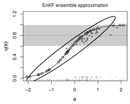
This produces a posterior ensemble for the joint distribution of $(\theta,\eta)$, given by the gray dots in the right hand frame of Figure 3. Hence the difference between these two representations can be seen Figure 3 – compare the gray ellipse in the left frame, representing the updated normal posterior, to the gray dots in the right frame, representing draws using this ensemble representation.

Note that if we take $(\theta^{\circ}_{k},\eta^{\circ}_{k})$ to be a draw from a distribution with mean $\mu_{\rm pr}$ and variance $\Sigma_{\rm pr}$, applying (7) – or equivalently (8) – produces a random variable $(\theta^{(1)}_{k},\eta^{(1)}_{k})$ with mean and variance given in (6) and (5). Hence the mean and variance of the ensemble members $(\theta^{(1)}_{k},\eta^{(1)}_{k})$ matches that of the Gaussian representation of the EnKF (4). Even though the first and second moments of the two EnKF representations match in distribution, the ensemble representation appears to better capture the true, right skewed posterior (compare to Figure 1).

A two-stage approach

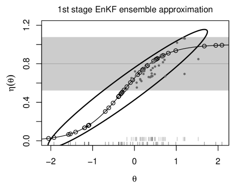
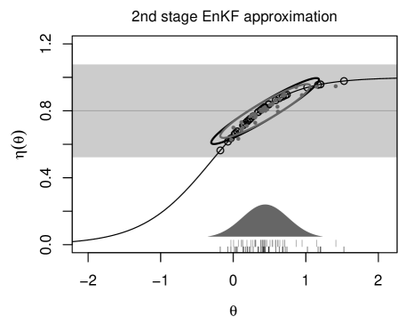
Figure 4 shows how one can repeatedly apply the EnKF to improve the accuracy of the of the normal representation of $\eta(\theta)$ where the posterior mass for $\theta$ is concentrated. This iterative strategy is closer to the original use of the EnKF for state-space estimation in non-linear, dynamic systems. Also, this two stage approach easily generalizes to additional stages.

For this two-stage EnKF, we artificially break the information from the likelihood into two even pieces

$$L(y|\eta(\theta))\propto\exp\left\{-\frac{1}{2}\frac{1}{(2\sigma_{y}^{2})}(y-\eta(\theta))^{2}\right\}\times\exp\left\{-\frac{1}{2}\frac{1}{(2\sigma_{y}^{2})}(y-\eta(\theta))^{2}\right\}$$

as if $y$ were observed twice, with twice the error variance. Then the EnKF is first applied to one of these $y$ values, with twice the error varriance, producing an ensemble representation $\theta^{(1)}_{1},\ldots,\theta^{(1)}_{m}$ of the posterior distribution for $\theta$ given this partial piece of information. Next, the forward model is run again at each of these new parameter settings, producing the ensemble $(\theta^{(1)}_{k},\eta(\theta^{(1)}_{k})),\;k=1,\ldots,m$. This new ensemble is now the starting point for a second EnKF update, again using $y$ with twice the error variance.

This second update can produce a Gaussian representation (the gray ellipse in the right frame of Figure 4), or an ensemble representation $(\theta^{(2)}_{k},\eta^{(2)}_{k}),\;k=1,\ldots,m$ (the gray dots in the right frame of Figure 4). As can be seen in the right frame of Figure 4, the second Gaussian representation of the relationship between $\theta$ and $\eta(\theta)$ is more accurate because the $(\theta^{(1)},\eta(\theta^{(1)}))$ ensemble covers a narrower range, over which $\eta(\theta)$ is more nearly linear.

Clearly, the choice of using two even splits of the likelihood information is somewhat arbitrary – both the number of splits and the partitioning of information to each split could be made in many ways. The cost of additional forward model evaluations has to be weighed against the benefits of a slightly more accurate Gaussian representation of $\eta(\theta)$ over a restricted range of values for $\theta$.

Figure 4: A two-stage EnKF solution to the simple inverse problem. Here the EnKF is applied twice, using the same observation $y$, but assuming it is observed with twice the variance. Left: at the first stage, the ensemble representation is used, assuming the observation has twice the variance, giving a data uncertainty that is a factor of $\sqrt{2}$ larger than in the previous figures. Right: the second stage starts with the updated ensemble, evaluatingng the forward model at each $\theta^{(1)}_{k}$, producing a new ensemble $(\theta^{(1)}_{1},\eta(\theta^{(1)}_{1})),\ldots,(\theta^{(1)}_{m},\eta(\theta^{(1)}_{m}))$. This new ensemble is updated once more, again using the data with twice the variance. The resulting uncertainty can be represented with a Gaussian distribution (shaded density) or an ensemble $(\theta^{(2)}_{1},\eta^{(2)}_{1}),\ldots,(\theta^{(2)}_{m},\eta^{(2)}_{m})$ (shaded dots).

1.1.3 Embedding the EnKF into a Bayesian formulation

As noted in a number of references (Anderson and Anderson, , 1999; Shumway and Stoffer, , 2010; Stroud et al., , 2010), the EnKF can be embedded in a likelihood or Bayesian formulation. For this simple inverse problem lends itself to the Bayesian formulation below,

$$\mbox{sampling model: }y|\eta(\theta) \sim N(\eta(\theta),\sigma_{y}^{2})$$

$$\mbox{prior model: }(\theta,\eta) \sim N(\mu_{\rm pr},\Sigma_{\rm pr}),$$

or, equivalently

$$y|\eta(\theta) \sim N(\eta(\theta),\sigma_{y}^{2})$$

$$\eta|\theta \sim N\left(\mu_{{\rm pr}2}+\Sigma_{{\rm pr}22}^{-1}\Sigma_{{\rm pr}21}(\theta-\mu_{{\rm pr}1}),\Sigma_{{\rm pr}22}-\Sigma_{{\rm pr}21}\Sigma_{{\rm pr}11}^{-1}\Sigma_{{\rm pr}12}\right)$$

$$\theta \sim N(\mu_{{\rm pr}1},\Sigma_{{\rm pr}11}).$$

In looking at the prior specification of $\eta|\theta$ above, it’s apparent that the mean is just the linear regression estimate of $\eta$ given $\theta$. Hence where a GP model is used in the formulation described in Figure 2, the EnKF implicitly uses a linear regression-based emulator. While this simple form can only account for linear effects and no interactions, the tradeoff is that this emulator can be estimated quickly, can handle large ensemble sizes $m$, and can handle moderately high-dimensional input parameter, and output spaces.

The EnKF uses the initial sample of model runs $(\theta^{\circ}_{1},\eta(\theta^{\circ}_{1})),\ldots,(\theta^{\circ}_{m},\eta(\theta^{\circ}_{m}))$ to produce the standard plug-in estimates for $\mu_{\rm pr}$ and $\Sigma_{\rm pr}$ – the sample mean and covariance. In static inverse problems, where quick turn-around of results isn’t crucial, one could specify priors for these parameters, producing a more fully Bayesian solution. An obvious choice might take vague, normal prior for $\mu_{\rm pr}$, and an inverse wishart for $\Sigma_{\rm pr}$ (West and Harrison, , 1997), if $m$ is sufficiently large relative to the dimensionality of $y$ and $\theta$.

In cases where the dimensionality of $\mu_{\rm pr}$ and $\Sigma_{\rm pr}$ is large (much larger than the ensemble size $m$) covariance tapering, or some other form of localization is used to deal with spurious correlations produced in the standard sample covariance estimate (Furrer and Bengtsson, , 2007; Evensen, , 2009b; Stroud et al., , 2010). The above specification suggests the use of variable selection (Wasserman, , 2000; Tibshirani, , 1996), or compressed sensing (Baraniuk, , 2007) could make a viable alternative for estimating the regression function for $\eta$ given the ensemble draws for $\theta$, producing the updated ensemble. Finally, we note that a bootstrap could be a useful tool for accounting for the uncertainty in the ensemble-based estimates for $\mu_{\rm pr}$ and $\Sigma_{\rm pr}$ since it does not require any additional model runs be carried out.

2 Applications

This section describes three applications in the statistical analysis of computer models that make use of the EnKF. The first two are calibration examples, one taken from cosmology, the second from climate. The last explores how this EnKF representation can be used to for experimental design, determining optimal spatial locations at which to take ice sheet measurements. The goal of these examples are to suggest possible uses of EnKF ideas, rather than providing definitive analyses in problems involving inference with the aid of computationally demanding computer models.

2.1 Calibration of cosmological parameters

Perhaps the simplest cosmological model in agreement with available physical observations (e.g. the large scale structure of the universe, the cosmic microwave background) is the $\Lambda$-cold dark matter ($\Lambda$CDM) model. This model, controlled by a small number of parameters, determines the composition, expansion and fluctuations of the universe.

This example focuses on model calibration, combining observations from the Sloan Digital Sky Survey (Adelman-McCarthy et al., , 2006), giving a local spatial map of large galaxies, with large-scale $N$-body simulations, controlled by five $\Lambda$CDM model parameters, evolving matter over a history that begins with the big bang, and ends at our current time, about 14 billion years later. An example of the physical observations produced by the SDSS are shown in the left frame of Figure 5. It shows a slice of the 3-d spatial map of large galaxies. Along with spatial position, the estimated mass for each of galaxy is also recorded.

The computational model predicts the current spatial distribution of matter in the universe, given the parameters of the $\Lambda$CDM model, requiring substantial computing effort. For a given parameter setting, a very large-scale $N$-body simulation is carried out. The simulation initializes dark matter tracer particles according to the cosmic microwave background and then propagates them according to gravity and other forces up to the present time. The result of one such simulation is shown in the middle frame of Figure 5. Different cosmologies (i.e. cosmological parameter settings) yield simulations with different spatial structure. We would like to determine which cosmologies are consistent with physical observations of the SDSS given in the left frame of Figure 5.

Figure 5: Left: Physical observations from the Sloan Digital Sky Survey (Credit: Sloan Digital Sky Survey). Middle: Simulation results from an $N$-body simulation. Right: Power spectra for the Matter density fields. The gray lines are from 128 simulations; the black lines give spectrum estimates derived from the physical observations.

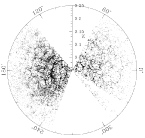
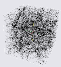
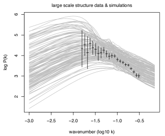
Direct comparison between the simulation output and the SDSS data is not possible since the simulations evolve an idealized, periodic cube of particles corresponding to clusters of galaxies, while the SDSS data give a censored, local snapshot of the large scale structure of the universe. Instead, we summarize the simulation output and physical observations by their dark matter power spectra which describe the spatial distribution of matter density at a wide range of length scales.

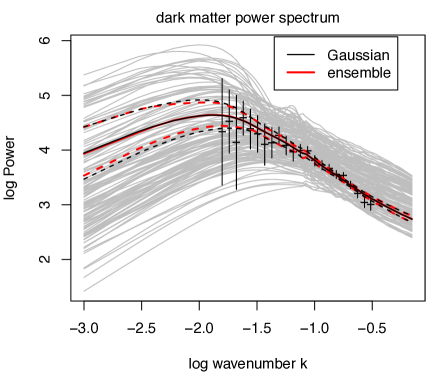
Computing the matter power spectrum is trivial for the simulation output since it is defined on a periodic, cubic lattice. In contrast, determining matter power spectrum from the SDSS data is a far more challenging task since one must account for the many difficulties that accompany observational data: nonstandard survey geometry, redshift space distortions, luminosity bias and noise, just to name a few. Because of these challenges, we use the published data and likelihood of Tegmark et al., (2004) which is summarized by the black lines in the right hand frame of Figure 5. The resulting data correspond to 22 pairs $(y_{i},k_{i})$ where $y_{i}$ is a binned estimate of the log of the power, and $k_{i}$ denotes the wavenumber corresponding to the estimate. The data vector $y=(y_{1},\ldots,y_{22})^{\prime}$ has a diagonal covariance $\Sigma_{y}$. Two standard deviation error bars are shown in the right frame of Figure 5 for each observation.

We take the ensemble produced in Heitmann et al., (2006) – a $m=128$ run orthogonal array-based latin hypercube sample (LHS) over the 5-d rectangular parameter space detailed in Table 1. Since this sample was originally generated to produce a multivariate GP emulator – predicting the simulated matter power spectrum as a function of the 5-d parameter inputs – it is not a draw from a normal prior as is standard for EnKF applications. Nevertheless, this sample can be used to estimate $\mu_{\rm pr}$ and $\Sigma_{\rm pr}$ from Section 1.1.2. The restricted ranges of the parameters will need to be reconciled with the eventual normal description of the parameter posterior, or resulting EnKF sample.

Table 1: $\Lambda$CDM parameters and their lower and upper bounds.

parameter description lower upper $n$ spectral index 0.8 1.4 $h$ Hubble constant 0.5 1.1 $\sigma_{8}$ galaxy fluctuation amplitude 0.6 1.6 $\Omega_{\rm CDM}$ dark matter density 0.0 0.6 $\Omega_{\rm B}$ baryonic matter density 0.02 0.12

For each of the $m=128$ parameter settings prescribed in the LHS, the simulation produces a 55-vector of log power spectrum outputs, given by the gray lines in the right hand frame of Figure 5. Of the 55 elements in the simulation output vector, 22 of the elements are at the wavenumber $k$ corresponding to the physical observations. Concatenating the parameter settings with the with the simulation output produces $m=128$ vectors of length $5+55$

$$\begin{pmatrix}\theta_{k}^{\circ}\\ \eta(\theta^{\circ}_{k})\end{pmatrix},\,k=1,\ldots,m.$$

We take $H$ to be the $22\times 60$ incidence matrix, selecting the elements of the vector $(\theta^{\circ},\eta(\theta^{\circ}))$ that correspond to the physical observations. This, along with the physical observations $y$ and corresponding measurement covariance $\Sigma_{y}$ are the necessary inputs to carry out the Gaussian and ensemble representations of the EnKF described in Sections 1.1.2.

The estimates of the posterior distribution for the 5-dimensional parameter vector is shown in the left frame of Figure 6. The presence of some slight skewness is noticible in the estimate produced by the ensemble representation. Also produced in these two estimation schemes is an estimate of the fitted log power spectrum, along with uncertainties, given in the right frame of Figure 6.

Figure 6: The estimated posterior distribution for the model parameters (left) and the log power (right). Left: One- and two-dimensional marginals for the estimated posterior for the cosmological parameters. The upper triangle shows the 128 updated ensemble members (light circle plotting symbols) and a sample from the Gaussian representation (black dots). The lower triangle shows estimated 90% hpd contours for both the ensemble (light lines) and Gaussian representations (black lines). Right: posterior mean and pointwise 90% credible bands for log power spectrum for the matter density of the universe. Light lines give the estimate produced by the ensemble representation; black lines give the estimate produced by the Gaussian representation.

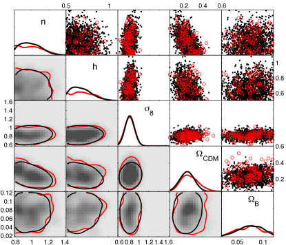
These results, produced by the EnKF, can be compared to the posterior in Higdon et al., (2010), which was produced using a multivariate GP emulator, with a far more elaborate statistical formulation. The resulting posteriors are similar, but both EnKF estimates seem to “chop off” tails in the posterior for the cosmological parameters that are present in the GP emulator-based analysis.

2.2 Optimal location of ice sheet measurements

This second application comes from an ongoing effort to use the community ice sheet model (CISM) (Rutt et al., , 2009; Price et al., , 2011) along with physical measurements to better understand ice sheet behavior and its impact on climate. This study considers a model of an idealized ice sheet over a rectangular region which is flowing out to sea on one side, while accumulating ice from prescribed precipitation over a time of 1000 years. This implementation of the CISM depends on two parameters – $\theta_{1}$ a constant in the Glen-Nye flow law (Greve and Blatter, , 2009), controlling the deformation of the ice sheet, and $\theta_{2}$ which controls the heat conductivity in the ice sheet. A few time snapshots of the model output are shown in Figure 7 for a particular choice of model parameters $\theta_{1}$ and $\theta_{2}$.

Figure 7: Output from the idealized ice sheet model. The idealized ice sheet is described by height over a 36m $\times$ 30m base, bounded on three sides by ledges. The fourth side is open to the ocean. Over the span of 1000 years, the ice flows into the ocean, while being replenished by a prescribed precipitation. Of interest in this application is the thickness of the ice sheet at 1000 years.

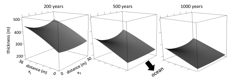
While this configuration does not realistically represent important ice sheets in Greenland or Antarctica, it is a testbed where methodology can be evaluated for model calibration and/or planing measurement campaigns. After 1000 years, the thickness of the ice sheet could be measured to inform about the model parameters $\theta_{1}$ and $\theta_{2}$. The goal of this application is to use an ensemble of $m=20$ model runs at different $\theta=(\theta_{1},\theta_{2})$ input settings to find a best set of 5 or 10 locations at which to measure the ice sheet thickness.

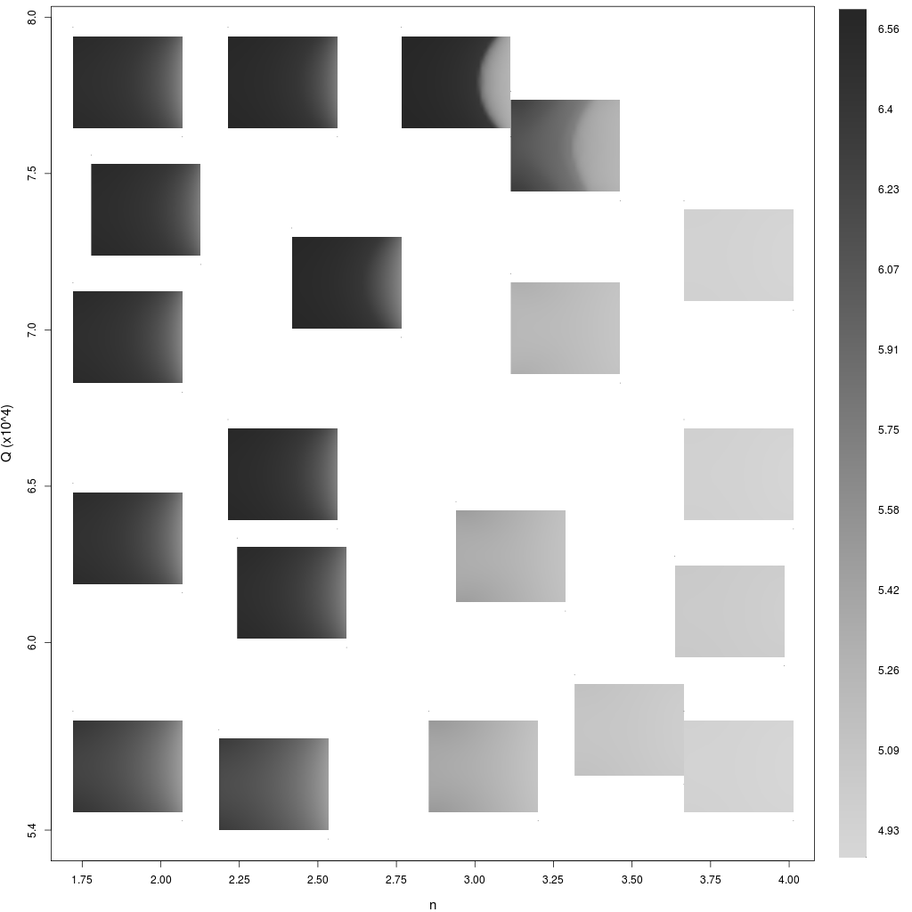
The parameter settings and resulting ice sheet thickness (after 1000 years) for the $m=20$ model runs are shown in Figure 8. Thickness is produced on a $36\times 30$ rectangular lattice of spatial locations. From this figure it’s clear that the modeled ice sheet thickness is larger for smaller values of $\theta_{1}$, and larger values of $\theta_{2}$.

Figure 8: Output from the ensemble of 20 model runs, showing thickness of the ice sheet after 1000 years, plotted in the $(\theta_{1},\theta_{2})$-parameter space. $\theta_{1}$ controls deformation of the ice sheet; $\theta_{2}$ controls heat conductivity in the ice sheet. Each image shows thickness as a function of spatial location; the center of the image marks the $(\theta_{1},\theta_{2})$ input setting at which the model was run. The grayscale indicates log thickness.

The model runs produce an ensemble of $2+36\cdot 30=p$-vectors $(\theta_{k},\eta(\theta_{k}))$, $k=1,\ldots,m$. We consider $n$ ice thickness measurements taken at $n$ of the $36\cdot 30$ spatial grid locations given by the model. A given set of $n$ measurement locations, is indexed by the $n\times p$ incidence matrix $H$, which will contain a single 1 in each of its $n$ rows. Thus there are $\binom{n}{p-2}$ possible measurement designs under consideration, each determined by which of the last $p-2$ columns of $H$ contain a 1.

We use the Gaussian representation of the EnKF to describe the resulting uncertainty in $\theta$, giving a simple means to compare designs which are determined by $H$. Assuming the $n$ thickness measurements have independent measurement errors, with a standard deviation of one meter, means $\Sigma_{y}$ is the $n\times n$ identity matrix. Then the resulting posterior variance for the joint parameter-output vector is given by (5)

$$\Sigma_{\rm post}^{-1}=\Sigma_{\rm pr}^{-1}+H^{\prime}\Sigma_{y}^{-1}H,$$

with the upper $2\times 2$ submatrix of $\Sigma_{\rm post}$ describing the posterior variance for the parameter vector $\theta$.

The sample covariance estimate for $\Sigma_{\rm pr}$, estimated from only $m=20$ model runs, gives some spurious estimates for the elements of the covariance matrix, leading to aberrant behavior in estimates for conditional mean and variance for $\theta$ given $\eta$. If we define

$$\mu_{\rm pr}=\begin{pmatrix}\mu_{\theta}\\ \mu_{\eta}\end{pmatrix}\mbox{ and }\Sigma_{\rm pr}=\begin{pmatrix}\Sigma_{\theta\theta}&\Sigma_{\theta\eta}\\ \Sigma_{\eta\theta}&\Sigma_{\eta\eta}\end{pmatrix},$$ (9)

corresponding to the 2-vector $\theta$ and the $p-2$-vector $\eta$, a spatial tapering covariance matrix $R(r)$ can be used to help stabilize these estimates (Kaufman et al., , 2008; Furrer and Bengtsson, , 2007) Hence we can produce an improved estimate

$$\Sigma_{\eta\eta}(r)=S\circ R(r)$$

where $S$ denotes the sample covariance matrix from the samples $\eta_{1},\ldots,\eta_{m}$, and $\circ$ denotes the elementwise product of the matrix elements. Here we take $R(r)$ to be the spatial correlation matrix induced by the isotropic exponential correlation function, with a correlation distance of $r$. The value for $r$ is taken to be the maximizer of the likelihood of prior samples $\eta_{1},\ldots,\eta_{m}$.

$$L(r)\propto\prod_{k=1}^{m}|\Sigma_{\eta\eta}(r)|^{-\frac{1}{2}}\exp\left\{-\frac{1}{2}\left(\eta_{k}-\mu_{\eta}\right)^{\prime}\Sigma_{\eta\eta}^{-1}\left(\eta_{k}-\mu_{\eta}\right)\right\}$$

Using this plug-in estimate for $r$, and treating $\Sigma_{\rm pr}$ as known, the Bayesian $D$-optimal design that maximizes the prior-posterior gain Shannon information is simply the $H$ that minimizes the determinant of the $\Sigma_{\rm post}^{\theta}$ – the upper $2\times 2$ submatrix of $\Sigma_{\rm post}$ (Chaloner and Verdinelli, , 1995).

Of course, since only a small number $n$ of observations are likely to be taken, one need not compute using the full $p\times p$ matrix $\Sigma_{\rm post}$. If we define $H_{\eta}$ to be the $n\times(p-2)$ restriction of $H$, removing the first two columns of $H$, then the posterior covariance matrix for $\theta$ can be written

$$\Sigma^{\theta}_{\rm post}=\Sigma_{\theta\theta}-\Sigma_{\theta\eta}H^{\prime}_{\eta}(H_{\eta}\Sigma_{\eta\eta}(r)H^{\prime}_{\eta}+\Sigma_{y})^{-1}H_{\eta}\Sigma_{\eta\theta}.$$

Here the computations require only the solve of a relatively small $n\times n$ system.

Figure 9: Estimates of the Bayesian $D$-optimal designs for locations at which to measure the ice sheet depth for $n=3$, 5, and 10. The estimates use a plug-in estimate for the spatial covariance distance of the covariance taper matrix, and Federov’s exchange algorithm to carry out the optimization.

We use the exchange algorithm of Fedorov, (1972) to search for the design $H_{\eta}$ that approximately minimizes the determinant of $\Sigma^{\theta}_{\rm post}$. The estimated optimal sampling locations for depth measurements with $n=3$, 5, and 10, are shown in Figure 9. While the optimization algorithm only guarantees a local maximum, we tried a large number of restarts, with the configurations giving the minimal determinant of $\Sigma_{\rm post}^{\theta}$ shown in Figure 9.

2.3 Calibration of parameters in the Community Atmosphere Model

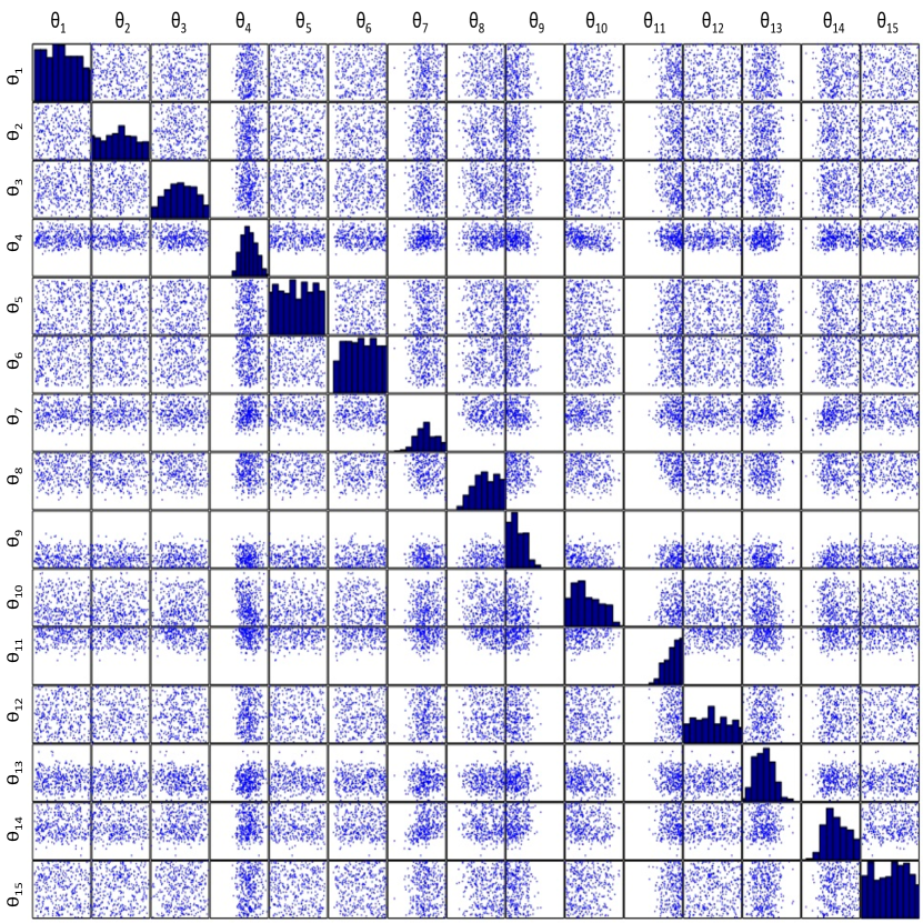
This final application is an adaptation of the application described in Jackson et al., (2008), in which multiple very fast simulated annealing (MVFSA) was used to approximate the posterior distribution of climate model parameters. Here we use the EnKF to carry out model calibration, considering a more recent ensemble of 1,400 model runs, using the community atmosphere model CAM 3.1, as described in Jackson et al., (2008). In this application 15 model parameters are sampled uniformly over a 15-dimensional rectangle whose ranges are apparent in Figure 11. The model parameters, output fields, and corresponding physical observation fields are listed in Table 2.

Table 2: Climate model inputs, outputs and physical data

inputs outputs and physical data description description $\theta_{1}$ effective radius of liquid cloud droplets over sea ice $\eta_{1},y_{1}$ shortwave cloud forcing $\theta_{2}$ cloud particle number density over ocean & land $\eta_{2},y_{2}$ precipitation over ocean $\theta_{3}$ effective radius of liquid cloud droplets over land $\eta_{3},y_{3}$ two meter air temperature $\theta_{4}$ time scale for consumption rate of deep CAPE $\eta_{4},y_{4}$ zonal winds at 300mb $\theta_{5}$ cloud particle number density over warm land $\eta_{5},y_{5}$ vertically averaged relative humidity $\theta_{6}$ threshold for autoconversion of warm ice $\eta_{6},y_{6}$ air temperature $\theta_{7}$ threshold for autoconversion of cold ice $\eta_{7},y_{7}$ latent heat flux over ocean $\theta_{8}$ effective radius of liquid cloud droplets over ocean $\theta_{9}$ environmental air entrainment rate $\theta_{10}$ initial cloud downdraft mass flux $\theta_{11}$ low cloud relative humidity $\theta_{12}$ ice fall velocities $\theta_{13}$ low cloud relative humidity $\theta_{14}$ deep convection precipitation efficiency $\theta_{15}$ cloud particle number density over sea ice

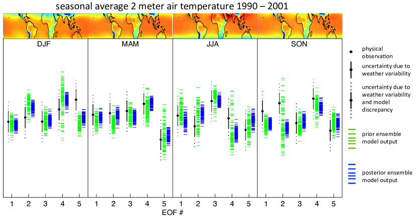
The computational model, described in detail in Jackson et al., (2008), produces a large number of outputs that could be compared to physical observations. We focus on a subset of the outputs (listed in Table 2) explored in the original investigation. Each of these outputs is recorded as a field over the globe, averaged over 11 years (from 1990 to 2001), separately for each season (December – February, DJF; March – May, MAM; June – August, JJA; September – November, SON) . The images in Figure 10 show the two-meter air temperature observations.

Rather that work directly with the model output and observed fields, we project these fields onto a precomputed empirical orthogonal function (EOF) basis, producing a small vector of weights – one for each basis function – to represent each field (von Storch and Zwiers, , 1999). As in Jackson et al., (2008), the EOF bases are computed from a long pilot run, separately from any of the model runs used to make the ensemble. The resulting weights for the two-meter air temperature are shown by the light/green dashes (model) and the black dots (observation) in Figure 10. We use 5 EOF basis elements for each output-season combination. Thus the model output $\eta$ and observation fields $y$ are each summarized by a $7\times 4\times 5$ vector of weights, corresponding to output, season, and EOF basis respectively.

The long pilot run is also used to estimate the variation in the outputs expected just due to variation in climate. Thus for each output, season, and EOF, a variance $\sigma^{2}_{\rm clim}$ is also estimated. We scale the EOF bases so that each $\sigma^{2}_{\rm clim}$ is estimated to be 1. Thus, the error bars in Figure 10 are $\pm 2$ because of this scaling. This scaling also makes the actual values of the $y$-axis in the figure essentially meaningless.

Figure 10: Physical observations and uncertainty (black), prior simulations (light/green), and posterior predictions (dark/blue) for seasonal 2-meter air temperature, averaged from 1990 to 2001. The averages are computed for each season (DJF = Dec, Jan, Feb, and so on). The observed and simulated temperature fields are projected onto five EOF basis functions for each season, producing five EOF weights for each field. The basis was estimated using a single, long pilot run. The black dot shows EOF weights corresponding to the physical observations, the solid black line shows a 2-$\sigma_{\rm clim}$ bound for climate variation computed from the pilot run; the dashed black lines show additional uncertainty due to the estimated discrepancy error. The light/green lines are a sample of outputs from the ensemble of model runs. The dark/blue lines give the corresponding ensemble representation for the updated (i.e. posterior) model predictions. The scale of the $y$-axis has been standardized so that the estimated climate variance is one for each of the basis weights. The images above the plots show the physically observed two-meter air temperature fields.

Even with this variation estimated from the pilot run, it is expected that there will still be a discrepancy between the physical observations and the model output, even at the best parameter setting $\theta$, for at least some of the outputs. Hence we specify $\Sigma_{y}$ to be the sum of the variance due to climate variation $I_{140}$ and a diagonal covariance matrix that accounts for this additional discrepancy $\Sigma_{\delta}$. For each output $i$ we allow a different precision $\lambda_{i}$ for the discrepancy that is common across seasons and EOF bases. This gives

$$\Sigma_{\delta}=\mbox{diag}\left(\lambda_{1}^{-1},\ldots,\lambda_{7}^{-1}\right)\otimes I_{20}$$

so that

$$\Sigma_{y}=I_{140}+\Sigma_{\delta}.$$

The black dotted lines in Figure 10 show this additional uncertainty due to model discrepancy for the 2 meter air temperature, governed by $\lambda_{3}$. We specify independent $\Gamma(a=1,b=.001)$ priors for each $\lambda_{i}$, $i=1,\ldots,7$.

In order to estimate these precision parameters, we note that the full 140-dimensional observation vector $y$ is modeled as the sum of normal terms

$$y=\eta+\epsilon_{\rm clim}+\epsilon_{\rm discrep}$$

where $\eta\sim N(\mu_{\eta},\Sigma_{\eta\eta})$, with $\mu_{\eta}$ and $\Sigma_{\eta\eta}$ estimated from the prior ensemble as defined in (9), $\epsilon_{\rm clim}\sim N(0,I_{140})$, and $\epsilon_{\rm discrep}\sim N(0,\Sigma_{\delta})$. If we define

$$V(\lambda)=\Sigma_{\eta\eta}+I_{140}+\Sigma_{\delta},$$

we get the posterior distribution for the 7-vector $\lambda$

$$\pi(\lambda|y) \propto |V(\lambda)|^{-\frac{1}{2}}\exp\left\{-\mbox{\small$\frac{1}{2}$}(y-\mu_{\eta})^{\prime}V(\lambda)^{-1}(y-\mu\eta)\right\}$$

$$\times\prod_{i=1}^{7}\lambda_{i}^{a-1}e^{-b\lambda_{i}}.$$

We use the posterior mean as plug-in estimates for $\lambda$, determining $\Sigma_{y}$.

Now, given the dimension reduction from using the EOF bases estimated from the pilot run, the estimate for $\Sigma_{y}$, and the 1400 member ensemble of $15+140$-vectors $(\theta,\eta(\theta))$, and the ensemble-based estimates $\mu_{\rm pr}$ and $\Sigma_{\rm pr}$, the updated posterior distribution for $\eta$ and $\theta$ is computed using the ensemble representation. The dark/blue dashes in Figure 10 show the posterior ensemble for the model outputs in the EOF weight space for the two meter air temperature. Figure 11 shows the posterior ensemble of parameter values $\theta$. The prior ensemble was sampled uniformly over the 15-dimensional rectangle depicted in the figure.

Figure 11: Ensemble representation for the posterior distribution of the 15 model parameters after conditioning on 9 data fields. The parameter settings for the initial ensemble are uniform over the 15-dimensional rectangle depicted here.

While the formulation presented here is very similar to that of Jackson et al., (2008), we used an additive discrepancy covariance matrix, with different precisions for each output type; theirs used a $\Sigma_{y}$ that is proportional to the estimated climate variation. Also, this analysis used fewer types of physical observations. The resulting posterior distribution for $\theta$ is similar, with a bit more posterior spread in this analysis. Also, the EnKF analysis requires only an ensemble of model runs, with no need for the sequential sampling required for MVFSA.

Finally, we point out that Annan et al., (2005) also use the EnKF to carry out parameter estimation on a climate model. That example uses a multi-stage estimation approach, collecting observations over ten successive years. That paper also uses synthetic observations so that $\Sigma_{y}$ can be specified without the need for estimation.

3 Discussion

This paper highlights a number of features of the EnKF from the perspective of model calibration and shows examples of how it can be used in a variety of applications. Implicitly, the EnKF uses a multiple linear regression emulator to model the mapping between model parameters and outputs. This makes it easy for this approach to handle large ensembles – often a challenge for approaches that use GP-based emulators – as well as model outputs that are noisy or random. This also suggests regression-based approaches for dealing with high-dimensional input and output spaces may be helpful in EnKF applications.

While the EnKF nominally starts with an initial ensemble from the prior distribution for $\theta$, it’s clear this prior will have little impact on the final results if the physical observations are fairly constraining, as in the examples presented here. The uniform designs used in the applications here have little impact on the posterior results.

The results depend far more on specifications for covariance matrices, and how a large covariance matrix is estimated from a relatively small ensemble of model runs. We used likelihood and Bayesian approaches for estimation of covariance parameters; a variety of alternative approaches exist in the literature (Tippett et al., , 2003; Stroud and Bengtsson, , 2007; Evensen, , 2009a; Stroud et al., , 2010; Kaufman et al., , 2008).

The resulting posterior distribution for $\theta$ tends to chop off tails that would be present in a more exact formulation. This is clear from comparing the analyses of the simple inverse problem laid out in Section 1.1. This is largely due to the linearity of the regression based emulator implicitly used in the EnKF. We have also seen this phenomena in the ice sheet and cosmology applications when comparing to calibration analyses based on more exacting GP emulators.

Finally we note that the ability of the EnKF to quickly provide “rough and ready” results makes it ideal for more computationally demanding tasks such experimental design or other optimization problems that require many iterations of the estimation process. The ice sheet application of Section 2.2 is one such example.

References

- Adelman-McCarthy et al., (2006) Adelman-McCarthy, J., Agueros, M., Allam, S., Anderson, K., Anderson, S., Annis, J., Bahcall, N., Baldry, I., Barentine, J., Berlind, A., et al. (2006). “The Fourth Data Release of the Sloan Digital Sky Survey.” The Astrophysical Journal Supplement Series, 162, 1, 38–48.
- Aksoy et al., (2009) Aksoy, A., Dowell, D., and Snyder, C. (2009). “A multicase comparative assessment of the ensemble Kalman filter for assimilation of radar observations. Part I: Storm-scale analyses.” Monthly Weather Review, 137, 6, 1805–1824.
- Anderson, (2001) Anderson, J. (2001). “An ensemble adjustment Kalman filter for data assimilation.” Monthly weather review, 129, 12, 2884–2903.
- Anderson and Anderson, (1999) Anderson, J. and Anderson, S. (1999). “A Monte Carlo implementation of the nonlinear filtering problem to produce ensemble assimilations and forecasts.” Monthly Weather Review, 127, 12, 2741–2758.
- Annan et al., (2005) Annan, J., Hargreaves, J., Edwards, N., and Marsh, R. (2005). “Parameter estimation in an intermediate complexity earth system model using an ensemble Kalman filter.” Ocean Modelling, 8, 1-2, 135–154.
- Baraniuk, (2007) Baraniuk, R. (2007). “Compressive sensing [lecture notes].” Signal Processing Magazine, IEEE, 24, 4, 118–121.
- Bayarri et al., (2007) Bayarri, M. J., Berger, J. O., Paulo, R., Sacks, J., Cafeo, J. A., Cavendish, J., Lin, C., and Tu, J. (2007). “A Framework for Validation of Computer Models.” Technometrics, 49, 138–154.
- Chaloner and Verdinelli, (1995) Chaloner, K. and Verdinelli, I. (1995). “Bayesian experimental design: A review.” Statistical Science, 273–304.
- Christen and Fox, (2005) Christen, J. and Fox, C. (2005). “Markov Chain Monte Carlo Using an Approximation.” Journal of Computational & Graphical Statistics, 14, 4, 795–810.
- Craig et al., (2001) Craig, P. S., Goldstein, M., Rougier, J. C., and Seheult, A. H. (2001). “Bayesian Forecasting Using Large Computer Models.” Journal of the American Statistical Association, 96, 717–729.
- Efendiev et al., (2009) Efendiev, Y., Datta-Gupta, A., Ma, X., and Mallick, B. (2009). “Efficient sampling techniques for uncertainty quantification in history matching using nonlinear error models and ensemble level upscaling techniques.” Water Resources Research, 45, 11, W11414.
- Evensen, (2003) Evensen, G. (2003). “The ensemble Kalman filter: Theoretical formulation and practical implementation.” Ocean dynamics, 53, 4, 343–367.
- Evensen, (2009a) — (2009a). Data assimilation: the ensemble Kalman filter. Springer Verlag.
- Evensen, (2009b) — (2009b). “The ensemble Kalman filter for combined state and parameter estimation.” Control Systems Magazine, IEEE, 29, 3, 83–104.
- Fedorov, (1972) Fedorov, V. (1972). Theory of optimal experiments. Academic press.
- Furrer and Bengtsson, (2007) Furrer, R. and Bengtsson, T. (2007). “Estimation of high-dimensional prior and posterior covariance matrices in Kalman filter variants.” Journal of Multivariate Analysis, 98, 2, 227–255.
- Galbally et al., (2010) Galbally, D., Fidkowski, K., Willcox, K., and Ghattas, O. (2010). “Non-linear model reduction for uncertainty quantification in large-scale inverse problems.” International Journal for Numerical Methods in Engineering, 81, 12, 1581–1608.
- Ghanem and Doostan, (2006) Ghanem, R. and Doostan, A. (2006). “On the construction and analysis of stochastic models: characterization and propagation of the errors associated with limited data.” Journal of Computational Physics, 217, 1, 63–81.
- Greve and Blatter, (2009) Greve, R. and Blatter, H. (2009). Dynamics of ice sheets and glaciers. Springer Verlag.
- Heitmann et al., (2006) Heitmann, K., Higdon, D., Habib, S., and Nakhleh, C. (2006). “Cosmic Calibration.” Astrophyiscal Journal Letters, 646, L1.
- Higdon et al., (2010) Higdon, D., Heitmann, K., Nakhleh, C., and Habib, S. (2010). “Combining Simulations and Physical Observations to Estimate Cosmological Parameters.” In The Oxford Handbook of Applied Bayesian Analyses, eds. A. O’Hagan and M. West, 749–775. New York: Oxford University Press.
- Higdon et al., (2005) Higdon, D., Kennedy, M., Cavendish, J., Cafeo, J., and Ryne, R. D. (2005). “Combining field observations and simulations for calibration and prediction.” SIAM Journal of Scientific Computing, 26, 448–466.
- Houtekamer et al., (2005) Houtekamer, P., Mitchell, H., Pellerin, G., Buehner, M., Charron, M., Spacek, L., and Hansen, B. (2005). “Atmospheric data assimilation with an ensemble Kalman filter: Results with real observations.” Monthly Weather Review, 133, 3, 604–620.
- Jackson et al., (2008) Jackson, C., Sen, M., Huerta, G., Deng, Y., and Bowman, K. (2008). “Error reduction and convergence in climate prediction.” Journal of Climate, 21, 24, 6698–6709.
- Kaipio and Somersalo, (2004) Kaipio, J. P. and Somersalo, E. (2004). Statistical and Computational Inverse Problems. New York: Springer.
- Kaufman et al., (2008) Kaufman, C., Schervish, M., and Nychka, D. (2008). “Covariance tapering for likelihood-based estimation in large spatial data sets.” Journal of the American Statistical Association, 103, 484, 1545–1555.
- Kennedy and O’Hagan, (2001) Kennedy, M. and O’Hagan, A. (2001). “Bayesian calibration of computer models (with discussion).” Journal of the Royal Statistical Society (Series B), 68, 425–464.
- Lieberman et al., (2010) Lieberman, C., Willcox, K., and Ghattas, O. (2010). “Parameter and state model reduction for large-scale statistical inverse problems.” SIAM Journal on Scientific Computing.
- Mandel et al., (2004) Mandel, J., Chen, M., Franca, L., Johns, C., Puhalskii, A., Coen, J., Douglas, C., Kremens, R., Vodacek, A., and Zhao, W. (2004). “A note on dynamic data driven wildfire modeling.” Computational Science-ICCS 2004, 725–731.
- Marzouk and Najm, (2009) Marzouk, Y. and Najm, H. (2009). “Dimensionality reduction and polynomial chaos acceleration of Bayesian inference in inverse problems.” Journal of Computational Physics, 228, 6, 1862–1902.
- Meinhold and Singpurwalla, (1983) Meinhold, R. and Singpurwalla, N. (1983). “Understanding the Kalman filter.” American Statistician, 123–127.
- Moradkhani et al., (2005) Moradkhani, H., Sorooshian, S., Gupta, H., and Houser, P. (2005). “Dual state-parameter estimation of hydrological models using ensemble Kalman filter.” Advances in Water Resources, 28, 2, 135–147.
- Oliver and Chen, (2010) Oliver, D. and Chen, Y. (2010). “Recent progress on reservoir history matching: a review.” Computational Geosciences, 1–37.
- Price et al., (2011) Price, S., Payne, A., Howat, I., and Smith, B. (2011). “Committed sea-level rise for the next century from Greenland ice sheet dynamics during the past decade.” Proceedings of the National Academy of Sciences, 108, 22, 8978.
- Rutt et al., (2009) Rutt, I., Hagdorn, M., Hulton, N., and Payne, A. (2009). “The Glimmer community ice sheet model.” J. Geophys. Res, 114, F02004.
- Sacks et al., (1989) Sacks, J., Welch, W. J., Mitchell, T. J., and Wynn, H. P. (1989). “Design and Analysis of Computer Experiments (with Discussion).” Statistical Science, 4, 409–423.
- Shumway and Stoffer, (2010) Shumway, R. and Stoffer, D. (2010). Time series analysis and its applications: with R examples. Springer Verlag.
- Stroud and Bengtsson, (2007) Stroud, J. and Bengtsson, T. (2007). “Sequential state and variance estimation within the ensemble kalman filter.” Monthly Weather Review, 135, 9, 3194–3208.
- Stroud et al., (2010) Stroud, J., Stein, M., Lesht, B., Schwab, D., and Beletsky, D. (2010). “An ensemble Kalman filter and smoother for satellite data assimilation.” Journal of the American Statistical Association, 105, 491, 978–990.
- Szunyogh et al., (2008) Szunyogh, I., Kostelich, E., Gyarmati, G., Kalnay, E., Hunt, B., Ott, E., Satterfield, E., and Yorke, J. (2008). “A local ensemble transform Kalman filter data assimilation system for the NCEP global model.” Tellus A, 60, 1, 113–130.
- Tarantola, (2005) Tarantola, A. (2005). Inverse problem theory and methods for model parameter estimation. Society for Industrial Mathematics.
- Tegmark et al., (2004) Tegmark, M., Blanton, M., Strauss, M., Hoyle, F., Schlegel, D., Scoccimarro, R., Vogeley, M., Weinberg, D., Zehavi, I., Berlind, A., et al. (2004). “The Three-Dimensional Power Spectrum of Galaxies from the Sloan Digital Sky Survey.” The Astrophysical Journal, 606, 2, 702–740.
- Tibshirani, (1996) Tibshirani, R. (1996). “Regression shrinkage and selection via the lasso.” Journal of the Royal Statistical Society. Series B (Methodological), 267–288.
- Tippett et al., (2003) Tippett, M., Anderson, J., Bishop, C., Hamill, T., and Whitaker, J. (2003). “Ensemble square root filters.” Monthly Weather Review, 131, 1485–1490.
- Vernon et al., (2010) Vernon, I., Goldstein, M., and Bower, R. (2010). “Galaxy formation: a Bayesian uncertainty analysis.” Bayesian analysis., 5, 04, 619–670.
- von Storch and Zwiers, (1999) von Storch, H. and Zwiers, F. W. (1999). Statistical Analysis in Climate Research. New York: Cambridge University Press.
- Wasserman, (2000) Wasserman, L. (2000). “Bayesian model selection and model averaging.” Journal of Mathematical Psychology, 44, 1, 92–107.
- West and Harrison, (1997) West, M. and Harrison, J. (1997). Bayesian Forecasting and Dynamic Models (Second Edition). New York: Springer-Verlag.