Anomalous elasticity in a disordered layered XY model

Abstract

We investigate the effects of layered quenched disorder on the behavior of planar magnets, superfluids, and superconductors by performing large-scale Monte-Carlo simulations of a three-dimensional randomly layered XY model. Our data provide numerical evidence for the recently predicted anomalously elastic (sliding) intermediate phase between the conventional high-temperature and low-temperature phases. In this intermediate phase, the spin-wave stiffness perpendicular to the layers vanishes in the thermodynamic limit while the stiffness parallel to the layers as well as the spontaneous magnetization are nonzero. In addition, the susceptibility displays unconventional finite-size scaling properties. We compare our Monte-Carlo results with the theoretical predictions, and we discuss possible experiments in ultracold atomic gases, layered superconductors and in nanostructures.

I Introduction

Extended defects can be found in a wide variety of condensed matter systems. For example, realistic materials often contain one-dimensional and two-dimensional defects in the form of dislocation lines or grain boundaries. Recent progress in nano-technology also allows researchers to custom-design artificial structures with analogous properties. Extended defects in systems of ultracold atomic gases can be created by means of one-dimensional or two-dimensional disordered optical lattices.

Extended defects are larger than the usual finite-size impurities and are thus harder to “average out.” Consequently, they have a much greater influence on the thermodynamic behavior of the system in question. This was first established on the example of the McCoy-Wu model, a two-dimensional disordered classical Ising model whose disorder is perfectly correlated in one of the two dimensions, i.e., it takes the form of parallel line defects. McCoy and Wu McCoy and Wu (1968a, b, 1969); McCoy (1969) demonstrated in a series of papers that this model exhibits an exotic phase transition at which the magnetic susceptibility is infinite over an entire temperature range while the specific heat is smooth. Fisher Fisher (1992, 1995) later used a strong-disorder renormalization group to show that the critical point is of infinite-randomness type and is accompanied by strong (power-law) Griffiths singularities Griffiths (1969); Thill and Huse (1995); Guo et al. (1996); Rieger and Young (1996). Ising models with plane defects, i.e., with perfect disorder correlations in two rather than one dimensions display even stronger disorder effects: instead of being sharp, the phase transition is smeared over a range of temperatures Vojta (2003); Sknepnek and Vojta (2004).

The effective dimensionality of the defects forms the basis of a classification Vojta and Schmalian (2005); Vojta (2006) of phase transitions in systems with quenched disorder. Three classes can be distinguished: (i) If the defect dimensionality is below the lower critical dimension $d_{c}^{-}$ of the problem, the disordered system has a conventional critical point with exponentially weak Griffiths singularities. (ii) If the defect dimensionality is exactly equal to the lower critical dimension, the critical point of the disordered system is of infinite-randomness type and accompanied by strong power-law Griffiths singularities. (iii) If the defects are above the lower critical dimension, individual regions can order independently, leading to a smearing of the global phase transition.

The case of two-dimensional (planar) defects in systems with XY symmetry is of particular conceptual and experimental importance. Theoretically, XY systems with perfect disorder correlations in two dimensions are right at the boundary between cases (ii) and (iii) in the above classification. True long-range order on individual two-dimensional “slabs” is forbidden by the Mermin-Wagner theorem Mermin and Wagner (1966); however, these regions undergo a Kosterlitz-Thouless transition to a quasi long-range ordered phase Kosterlitz and Thouless (1973). Experimentally, order parameters with XY symmetry occur not only in planar magnets but also in superconductors and superfluids. The fate of the XY phase transition with two-dimensional defects is thus of great interest for magnetic and superconducting multilayers as well as ultracold atomic gases in one-dimensional disordered optical lattices.

Recently, two simultaneous publications Mohan et al. (2010a); Pekker et al. (2010) investigated this question theoretically. They predicted that the conventional high-temperature and low-temperature phases of a randomly layered XY system are separated by an anomalously elastic intermediate phase. In this exotic “sliding” phase which is part of the Griffiths region, the spin-wave (or superfluid) stiffness parallel to the layers is nonzero while the stiffness perpendicular to the layers vanishes.

In this paper, we report the results of large-scale Monte-Carlo simulations of a three-dimensional randomly layered XY model which provide support for the phase transition scenario predicted in Refs. Mohan et al. (2010a); Pekker et al. (2010). In particular, we give numerical evidence for existence of the anomalously elastic intermediate phase. Our paper in organized as follows. In Sec. II, we define the randomly layered XY model. We briefly summarize the theoretical predictions in Sec. III. Section IV is devoted to the Monte-Carlo simulations and their results. We conclude in Sec. V.

II Randomly layered XY model

In the following, we formulate the problem in the language of the XY ferromagnet. The results will apply to all phase transitions having O(2) or U(1) order parameters, if expressed in terms of the appropriate variables.

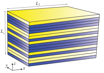
We consider a three-dimensional magnet consisting of a random sequence of layers made up of two different materials as shown in Fig. 1.

Figure 1: (Color online) Sketch of the layered XY model (1). Layers of two different materials (represented by different interaction strengths $J^{\parallel}$) are arranged in a random sequence.

Its Hamiltonian is a three-dimensional classical XY model defined on a lattice of perpendicular size $L_{\perp}$ (in the $z$ direction) and in-plane size $L_{\parallel}$ (in the $x$ and $y$ directions). It reads

$$H=-\sum_{\mathbf{r}}J^{\parallel}_{z}\,(\mathbf{S}_{\mathbf{r}}\cdot\mathbf{S}_{\mathbf{r}+\hat{\mathbf{x}}}+\mathbf{S}_{\mathbf{r}}\cdot\mathbf{S}_{\mathbf{r}+\hat{\mathbf{y}}})-\sum_{\mathbf{r}}J^{\perp}_{z}\,\mathbf{S}_{\mathbf{r}}\cdot\mathbf{S}_{\mathbf{r}+\hat{\mathbf{z}}}.$$ (1)

Here, $\mathbf{S}_{\mathbf{r}}$ is a two-component unit vector on lattice site $\mathbf{r}$, and $\hat{\mathbf{x}}$, $\hat{\mathbf{y}}$, and $\hat{\mathbf{z}}$ are the unit vectors in the coordinate directions. The interactions within the layers, $J^{\parallel}_{z}$, and between the layers, $J^{\perp}_{z}$, are both positive and independent random functions of the perpendicular coordinate $z$. For simplicity, we take all $J^{\perp}_{z}$ to be identical, $J^{\perp}_{z}\equiv J^{\perp}$ , while the $J^{\parallel}_{z}$ are drawn from a binary probability distribution

$$P(J^{\parallel})=(1-c)\,\delta(J^{\parallel}-J_{u})+c\,\delta(J^{\parallel}-J_{l})$$ (2)

with $J_{u}>J_{l}$. Here, $c$ is the concentration of the “weak” layers while $1-c$ is the concentration of the “strong” layers.

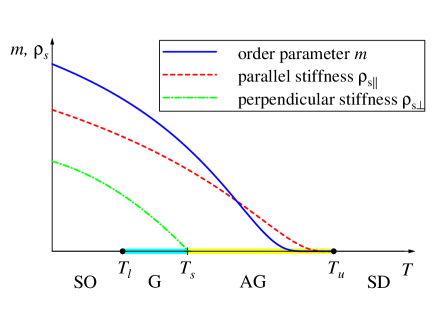
Let us discuss the thermodynamics of the randomly layered XY model (1) qualitatively. If the temperature $T$ is above the upper Griffiths temperature $T_{u}$ (defined as the critical temperature of a hypothetical clean system having $J^{\parallel}_{z}\equiv J_{u}$ for all $z$), the model is in a conventional paramagnetic phase (denoted “strongly disordered” in the phase diagram shown in Fig. 2).

Figure 2: (Color online) Schematic behavior of the order parameter (spontaneous magnetization) $m$ and the stiffnesses $\rho_{s,\parallel}$ and $\rho_{s,\perp}$ vs. temperature $T$ for any bounded disorder distribution. SD and SO denote the conventional strongly disordered and ordered phases, respectively. The Griffiths region (bounded by $T_{u}$ and $T_{l}$) consists of the “non-anomalous” (G) and the anomalous (AG) Griffiths phases. For an unbounded distribution, $T_{u}\rightarrow\infty$.

Analogously, for temperatures below the lower Griffiths temperature $T_{l}$ (defined as the critical temperature of a system having $J^{\parallel}_{z}\equiv J_{l}$ for all $z$), the model is in a conventional ferromagnetic (“strongly ordered”) phase. The most interesting temperature range is the Griffiths phase between $T_{u}$ and $T_{l}$. Here, rare thick slabs (rare regions) of strong ($J_{z}^{\parallel}=J_{u}$) layers can show local ferromagnetism while the bulk is still nonmagnetic. Individual such slabs cannot be truly long-range ordered Mermin and Wagner (1966) but they can develop quasi long-range order via individual Kosterlitz-Thouless phase transitions Kosterlitz and Thouless (1973). The exotic behavior predicted in Refs. Mohan et al. (2010a); Pekker et al. (2010) arises from the interplay between the quenched disorder and the Kosterlitz-Thouless physics of these strongly interacting slabs.

III Optimal fluctuation theory

In this section, we summarize the results of the optimal fluctuation theory of Ref. Mohan et al. (2010a). A slab (rare region) consisting of $L_{RR}$ consecutive strong layers exists with an exponentially small probability $w(L_{RR})\sim(1-c)^{L_{RR}}=\exp(-\tilde{c}L_{RR})$ with $\tilde{c}=-\ln(1-c)$. It undergoes a Kosterlitz-Thouless phase transition at a temperature $T_{KT}(L_{RR})$ which can be estimated from finite-size scaling via $T_{u}-T_{KT}\sim L_{RR}^{-1/\nu}$. (Here, $\nu\approx 0.6717$ Campostrini et al. (2006) is the correlation-length critical exponent of a clean 3D planar (XY) magnet.) Consequently, at a given temperature $T$, all rare regions of thickness $L_{RR}<L_{c}(T)\sim(T_{u}-T)^{-\nu}$ are (locally) in the paramagnetic phase while those having thicknesses $L_{RR}>L_{c}(T)$ are in the quasi-long-range ordered phase.

We first consider the behavior of a single rare region (slab) in the quasi-long-range ordered phase. According to Kosterlitz-Thouless theory Kosterlitz and Thouless (1973), its spin correlation function $C(\mathbf{r})$ decays as a non-universal power of the distance $|\mathbf{r}|$,

$$C(\mathbf{r})\sim|\mathbf{r}|^{-\eta}\qquad(|\mathbf{r}|\to\infty)~{}.$$ (3)

The exponent $\eta$ takes the value 1/4 right at the Kosterlitz-Thouless transition and behaves as $1/L_{RR}$ in the limit of $L_{RR}\to\infty$. Its thickness dependence can thus be modeled as $\eta(L_{RR})=\frac{1}{4}L_{c}(T)/L_{RR}$. The power-law correlations (3) lead to a nonlinear magnetization-field curve

$$m\sim H^{\eta/(4-\eta)}~{},$$ (4)

which implies that the magnetic susceptibility of a single slab in the quasi-long-range ordered phase is infinite.

We now turn to thermodynamic observables of the full, randomly layered system in the Griffiths phase $T_{u}>T>T_{l}$. The spin-wave stiffness $\rho_{s}$ is defined via the work required to twist the spins on two opposite boundaries of the sample by a relative angle $\theta$. In the limit of small $\theta$ and large system size, the free-energy density $f$ depends on $\theta$ as

$$f(\theta)-f(0)=\frac{1}{2}\rho_{s}\left({\theta}/{L}\right)^{2}$$ (5)

which defines $\rho_{s}$. As our randomly layered XY model is anisotropic, we need to distinguish the parallel spin-wave stiffness $\rho_{s}^{\parallel}$ from the perpendicular spin-wave stiffness $\rho_{s}^{\perp}$. To determine $\rho_{s}^{\parallel}$, we apply twisted boundary conditions at $x=0$ and $x=L_{\parallel}$ and set $L=L_{\parallel}$ in (5) while the boundary conditions are applied at $z=0$ and $z=L_{\perp}$ (using $L=L_{\perp}$) to find $\rho_{s}^{\perp}$.

When the twist is applied in $x$-direction, all layers in the sample have same boundary conditions. The total free energy cost due to the twist is thus simply given by a sum over all layers. As only slabs that are in the quasi-long-range ordered phase have a nonzero stiffness, the total parallel stiffness reads

$$\rho_{s,\parallel}\sim\int_{L_{c}(T)}^{\infty}dL_{RR}\,w(L_{RR})\,\rho_{s,RR}(L_{RR})~{}.$$ (6)

Here, $\rho_{s,RR}(L_{RR})$ is the (parallel) stiffness of a single slab of thickness $L_{RR}$. It is related to the value of the exponent $\eta$ via $\eta=T/(2\pi\rho_{s,RR})$. Because the probability $w(L_{RR})$ decays exponentially with increasing $L_{RR}$, the integral is dominated by its lower bound. To leading exponential accuracy, the parallel stiffness is thus given by

$$\rho_{s,\parallel}\sim\exp[-\tilde{c}L_{c}(T)]\sim\exp[-a\,(T_{u}-T)^{-\nu}]$$ (7)

with $a$ a non-universal constant. This means, it is non-zero anywhere in the Griffiths phase and develops an exponential tail towards $T_{u}$ (see Fig. 2).

When the twist $\theta$ is applied between the bottom ($z=0$) and the top ($z=L_{\perp}$) of the sample, the local twists between consecutive layers will vary from layer to layer. Minimizing the elastic free energy with respect to these local twists leads to

$$\rho_{s,\perp}\sim\langle 1/J_{\rm eff}^{\perp}\rangle^{-1}$$ (8)

where $J_{\rm eff}^{\perp}$ are the effective couplings between the rare regions, and $\langle\ldots\rangle$ is the average over the sample. Because the spatial positions of the rare regions are random, the distribution of their nearest-neighbor distances is a Poisson distribution, $P(R)=R_{KT}\exp(-R/R_{KT})$, where $R_{KT}\sim w(L_{c})^{-1}\sim\exp[\tilde{c}L_{c}(T)]$ is the typical separation. The effective interaction between neighboring rare regions decays exponentially, $J_{\rm{eff}}^{\perp}(R)\sim\exp(-R/\xi_{0})$, where $\xi_{0}$ is the bulk correlation length. We thus arrive at a power-law distribution

$$\bar{P}(J_{\rm{eff}}^{\perp})\sim(J_{\rm{eff}}^{\perp})^{1/z-1}~{}.$$ (9)

of the effective interactions. The Griffiths dynamical exponent $z\equiv R_{KT}/\xi_{0}$ takes the value $\infty$ at $T_{u}$, and decreases with decreasing temperature. Using this distribution, we find that the average $\langle 1/J_{\rm eff}^{\perp}\rangle$ diverges as long as $z>1$. This implies that the perpendicular stiffness $\rho_{s,\perp}$ vanishes in part of the Griffiths phase, viz., between $T_{u}$ and a temperature $T_{s}$ at which $z$ reaches the value $1$. In this temperature region, the elastic free energy density displays an anomalous dependence on the system size, $f(\Theta)-f(0)\sim L_{\perp}^{-1-z}$ corresponding to $\rho_{s,\perp}\sim L_{\perp}^{1-z}$. For $T<T_{s}$ the average $\langle 1/J_{\rm eff}^{\perp}\rangle$ converges, leading to a nonzero perpendicular stiffness. Close to $T_{s}$, the perpendicular stiffness is expected to behave as $\rho_{s,\perp}\sim T_{s}-T$ (see Fig. 2).

Other quantities can be found along the same lines Mohan et al. (2010a). For example, the spontaneous magnetization is nonzero for all $T<T_{u}$ and shows a double-exponential tail towards the nonmagnetic phase. Close to $T_{u}$, it takes the asymptotic form

$$\ln(m)\sim-\exp[a(T_{u}-T)^{-\nu}]~{},\qquad(T\to T_{u}-)~{}.$$ (10)

If a magnetic field $H$ is applied at temperatures $T\lesssim T_{u}$, the magnetization-field curve takes the unusual form

$$\ln(m)\sim-\sqrt{|\ln(H)|(T_{u}-T)^{-\nu}}~{},\qquad(H\to 0)~{},$$ (11)

for magnetizations larger than the double-exponentially small spontaneous magnetization (10).

For the comparison between theory and Monte-Carlo simulations, finite-size effects are an important issue. As an example, we discuss the dependence of the magnetic susceptibility in the Griffiths phase on the in-plane system size $L_{\parallel}$. When $L_{\parallel}$ is finite, the susceptibility of a single slab in the quasi-long-range ordered phase is no longer infinite. Its $L_{\parallel}$-dependence can be obtained from integrating the correlation function (3) to the upper cutoff $L_{\parallel}$ which results in $\chi_{RR}(L_{\parallel})\sim L_{\parallel}^{2-\eta}$. Summing this over all rare regions yields the total susceptibility (per unit volume) as

$$\chi\sim L_{\parallel}^{2}\exp\{-[\tilde{c}L_{c}(T)\ln(L_{\parallel})]^{1/2}\}~{}.$$ (12)

IV Monte-Carlo simulations

In this section, we report the results of Monte-Carlo simulations of the randomly layered XY model (1) by means of the highly efficient Wolff cluster algorithm Wolff (1989). To capture the physics of the rare regions, we have simulated large system sizes of up to $L_{\perp}=800$ and $L_{\parallel}=100$. In the binary distribution (2) for the in-plane interactions $J_{z}^{\parallel}$, we have chosen the values $J_{u}=1$ and $J_{l}=0.25$. All the simulations have been performed for an impurity concentration $c=0.8$. With these parameter choices, the Griffiths phase ranges from $T_{l}\approx 0.97$ to $T_{u}\approx 2.20$. All data are averages over a large number (from 100 to 300) of disorder realizations. For each realization we have used 100 Monte-Carlo (Wolff) sweeps for equilibration and another 100 sweeps for measurements.

To test the anomalous elastic properties predicted in part of the Griffiths phase, we have computed the parallel and perpendicular spin-wave stiffnesses. Finding the stiffnesses by actually performing simulation runs with twisted boundary conditions is not very efficient. However, the stiffnesses can be rewritten in terms of expectation values calculated in a conventional run with periodic boundary conditions. In the case of the perpendicular stiffness, the resulting formula Teitel and Jayaprakash (1983) (see also Hrahsheh et al. (2011)) reads

$$\rho_{s,\perp} = \frac{1}{N}\sum_{\langle\mathbf{r},\mathbf{r}^{\prime}\rangle}J_{\mathbf{r},\mathbf{r}^{\prime}}\langle\mathbf{S}_{\mathbf{r}}\cdot\mathbf{S}_{\mathbf{r}^{\prime}}\rangle(z-z^{\prime})^{2}$$

$$-\frac{1}{NT}\left\langle\left(\sum_{\langle\mathbf{r},\mathbf{r}^{\prime}\rangle}J_{\mathbf{r},\mathbf{r}^{\prime}}\,\hat{\mathbf{k}}\cdot(\mathbf{S}_{\mathbf{r}}\times\mathbf{S}_{\mathbf{r}^{\prime}})(z-z^{\prime})\right)^{2}\right\rangle~{},$$

where $N=L_{\perp}L_{\parallel}^{2}$ is the total number of sites, and $\hat{\mathbf{k}}$ is a unit vector perpendicular to the plane of the XY spins. For the calculation of $\rho_{s,\parallel}$, the term $(z-z^{\prime})$ needs to be replaced by $(x-x^{\prime})$.

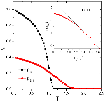
Using this formula, we have calculated the parallel and perpendicular stiffnesses of a system of sizes $L_{\perp}=800$ and $L_{\parallel}=100$. The results are shown in Fig. 3.

Figure 3: (Color online) Perpendicular and parallel spin-wave stiffnesses, $\rho_{s,\perp}$ and $\rho_{s,\parallel}$, as functions of temperature $T$ for a system with sizes $L_{\perp}=800$ and $L_{\parallel}=100$. The data are averaged over 100 disorder configurations. The inset shows that $\rho_{s,\parallel}$ follows the prediction (7) for $T\to T_{u}$.

The two stiffnesses clearly behave differently. The perpendicular stiffness $\rho_{s,\perp}$ vanishes at a temperature $T_{s}\approx 1.15$ while the parallel stiffness $\rho_{s,\parallel}$ remains nonzero to significantly higher temperatures and develops a tail towards $T_{u}$. In agreement with the theoretical predictions, we thus find an intermediate anomalously elastic (sliding) phase in which $\rho_{s,\perp}=0$ but $\rho_{s,\parallel}\neq 0$. To further test the theory, we plot $\ln(\rho_{s,\parallel})$ vs. $(T_{u}-T)^{-\nu}$ in the inset of Fig. 3. According to (7), the data sufficiently close to $T_{u}$ should fall onto a straight line. As the inset shows, our results follow the prediction over more than 1.5 orders of magnitude in $\rho_{s,\parallel}$ (down to the resolution limit set by the Monte-Carlo noise).

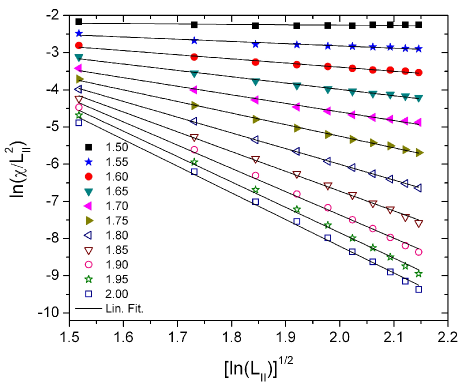
In addition to the spin-wave stiffnesses, we have also analyzed the finite-size behavior of the magnetic susceptibility. Figure 4 shows the susceptibility $\chi$ as a function of $L_{\parallel}$ for several temperatures in the Griffiths region.

Figure 4: (Color online) Susceptibility $\chi$ as a function of in-plane system size $L_{\parallel}$ for several temperatures in the Griffiths region. The perpendicular size is $L_{\perp}=800$; the data are averages over 300 disorder configurations. The solid lines are fits to the theoretical prediction (12).

We have used system sizes $L_{\perp}=800$ and $L_{\parallel}=10$ to $100$ because the condition $L_{\perp}\gg L_{\parallel}$ (such that $L_{\perp}$ is effectively infinite) needs to be fulfilled when studying the dependence of $\chi$ on $L_{\parallel}$.

To compare the simulations to the theory, we plot the Monte-Carlo data as $\ln(\chi/L_{\parallel}^{2})$ vs. $[\ln(L_{\parallel})]^{1/2}$. In such a plot, the functional form (12) yields a straight line. Figure 4 shows that our data are in good agreement with the theoretical prediction over a wide temperature range. Some deviations appear for temperatures close to $T_{u}$ and large $L_{\parallel}$. They are likely caused by the fact that the perpendicular size $L_{\perp}$ is not truly infinite in our simulations. Thus, a typical sample will not contain any of the very thick rare regions that dominate $\chi$ at temperatures close to $T_{u}$. From fits of the data to (12), one can obtain estimates of the cutoff length scale $L_{c}(T)$. Its temperature dependence does not agree very well with the prediction $L_{c}\sim(T_{u}-T)^{-\nu}$, probably because the theory holds asymptotically close to $T_{u}$ while the simulations for such temperatures suffer from the finite system size $L_{\perp}$, as discussed above.

V Conclusions

In summary, we have performed large-scale Monte-Carlo simulations of a classical three-dimensional XY model with layered randomness. Our results provide support for the recently predicted unconventional phase transition scenario Mohan et al. (2010a); Pekker et al. (2010). In particular, we have found evidence for the existence of an anomalously elastic (sliding) intermediate phase between $T_{u}$ and $T_{s}$. In this phase, the stiffness parallel to the layered randomness is nonzero while the perpendicular stiffness vanishes. We have also confirmed the unusual finite-size scaling behavior of the magnetic susceptibility.

It is interesting to compare the present results for a randomly layered XY model with corresponding results for Ising and Heisenberg spins. In a randomly layered Ising model, each rare region (slab) corresponds to a two-dimensional Ising model; it can thus undergo a transition to a long-range ordered state independently of the bulk system. The global phase transition is therefore smeared Vojta (2003); Sknepnek and Vojta (2004). (In the Ising case, the tail of the magnetization towards $T_{u}$ decays as a single exponential, i.e., $m$ is significantly larger than in the double exponential tail (10)). In contrast, for Heisenberg symmetry, the rare regions correspond to two-dimensional Heisenberg models which cannot develop long-range order independently. As a result, the global phase transition is sharp. However, the layered randomness leads to exotic infinite-randomness critical behavior Mohan et al. (2010b); Hrahsheh et al. (2011). In our case of the randomly layered XY model, the rare regions can undergo a phase transition independently from each other, but only to a quasi-long-range ordered state rather than to true long-range order. In terms of the classification Vojta and Schmalian (2005); Vojta (2006) of phase transitions in disordered systems, the randomly layered XY model is thus features a hybrid between a smeared and a sharp transition.

Turning to experiment, our results are applicable to a variety of systems. Even though our theory is formulated in the language of the planar (XY) ferromagnet, it holds for all thermal phase transitions with O(2) or U(1) order parameters, if it is expressed in terms of the appropriate variables. For randomly layered superconductors and superfluids, the magnetization should be exchanged for the Cooper pair amplitude or the condensate wave function. Analogously, the spin-wave stiffness should be substituted by the superfluid density. It is worth noting that recent large-scale quantum Monte-Carlo simulations of the Bose-Hubbard Hamiltonian on randomly stacked layers Laflorencie (2012) also confirmed the existence of an anomalously elastic (sliding) phase between the normal fluid and the superfluid in this system.

Experiments in ultracold atomic gases have already demonstrated the Kosterlitz-Thouless transition in stacks of quasi two-dimensional layers created by a strong one-dimensional optical lattice Hadzibabic et al. (2006). Moreover, disordered optical lattices have been used to study Anderson localization of matter waves Billy et al. (2008); Roati et al. (2008). Our results apply to large irregular stacks of quasi two-dimensional layers created by a one-dimensional disordered optical lattice of a strength that still allows some weak coupling between the layers.

Recently, experiments on several layered perovskite superconductors Li et al. (2007); Drachuck et al. (2011); Wen et al. (2012) found unexpected anisotropies of the superconducting properties that imply an apparent decoupling of the superconducting layers. Our anomalously elastic phase may explain these observations provided that there is sufficient c-axis disorder is the samples. Our theory could also be tested by manufacturing layered nanostructures of different magnetic or superconducting materials. Magnetic multilayers with systematic variations of the critical temperature from layer to layer have already been produced Marcellini et al. (2009). The system we have studied can be realized as a random version of such a structure using an easy-plane magnetic material.

References

- McCoy and Wu (1968a) B. M. McCoy and T. T. Wu, Phys. Rev. Lett. 21, 549 (1968a).
- McCoy and Wu (1968b) B. M. McCoy and T. T. Wu, Phys. Rev. 176, 631 (1968b).
- McCoy and Wu (1969) B. M. McCoy and T. T. Wu, Phys. Rev. 188, 982 (1969).
- McCoy (1969) B. M. McCoy, Phys. Rev. Lett. 23, 383 (1969).
- Fisher (1992) D. S. Fisher, Phys. Rev. Lett. 69, 534 (1992).
- Fisher (1995) D. S. Fisher, Phys. Rev. B 51, 6411 (1995).
- Griffiths (1969) R. B. Griffiths, Phys. Rev. Lett. 23, 17 (1969).
- Thill and Huse (1995) M. Thill and D. A. Huse, Physica A 214, 321 (1995).
- Guo et al. (1996) M. Guo, R. N. Bhatt, and D. A. Huse, Phys. Rev. B 54, 3336 (1996).
- Rieger and Young (1996) H. Rieger and A. P. Young, Phys. Rev. B 54, 3328 (1996).
- Vojta (2003) T. Vojta, J. Phys. A 36, 10921 (2003).
- Sknepnek and Vojta (2004) R. Sknepnek and T. Vojta, Phys. Rev. B 69, 174410 (2004).
- Vojta and Schmalian (2005) T. Vojta and J. Schmalian, Phys. Rev. B 72, 045438 (2005).
- Vojta (2006) T. Vojta, J. Phys. A 39, R143 (2006).
- Mermin and Wagner (1966) N. D. Mermin and H. Wagner, Phys. Rev. Lett. 17, 1133 (1966).
- Kosterlitz and Thouless (1973) J. M. Kosterlitz and D. J. Thouless, J. Phys. C 6, 1181 (1973).
- Mohan et al. (2010a) P. Mohan, P. M. Goldbart, R. Narayanan, J. Toner, and T. Vojta, Phys. Rev. Lett. 105, 085301 (2010a).
- Pekker et al. (2010) D. Pekker, G. Refael, and E. Demler, Phys. Rev. Lett. 105, 085302 (2010).
- Note (1) The full disordered phase transition scenario emerges even if only one of the two interactions, and , is random because the other interaction picks up randomness under renormalization.
- Campostrini et al. (2006) M. Campostrini, M. Hasenbusch, A. Pelissetto, and E. Vicari, Phys. Rev. B 74, 144506 (2006).
- Wolff (1989) U. Wolff, Phys. Rev. Lett. 62, 361 (1989).
- Teitel and Jayaprakash (1983) S. Teitel and C. Jayaprakash, Phys. Rev. B 27, 598 (1983).
- Hrahsheh et al. (2011) F. Hrahsheh, H. Barghathi, and T. Vojta, Phys. Rev. B 84, 184202 (2011).
- Mohan et al. (2010b) P. Mohan, R. Narayanan, and T. Vojta, Phys. Rev. B 81, 144407 (2010b).
- Laflorencie (2012) N. Laflorencie, (2012), arXiv:1204.0721 .
- Hadzibabic et al. (2006) Z. Hadzibabic, P. Krüger, M. Cheneau, B. Battelier, and J. Balibard, Nature 441, 1118 (2006).
- Billy et al. (2008) J. Billy, V. Josse, Z. Zuo, A. Bernard, B. Hambrecht, P. Lugan, D. Clément, L. Sanchez-Palencia, P. Bouyer, and A. Aspec, Nature 453, 891 (2008).
- Roati et al. (2008) G. Roati, C. D’Errico, L. Fallani, M. Fattori, C. Fort, M. Zaccanti, G. Modugno, M. Modugno, and M. Inguscio, Nature 453, 895 (2008).
- Li et al. (2007) Q. Li, M. Hücker, G. D. Gu, A. M. Tsvelik, and J. M. Tranquada, Phys. Rev. Lett. 99, 067001 (2007).
- Drachuck et al. (2011) G. Drachuck, M. Shay, G. Bazalitsky, J. Berger, and A. Keren, (2011), arXiv:1111.0470 .
- Wen et al. (2012) J. Wen, Q. Jie, Q. Li, M. Hücker, M. v. Zimmermann, S. J. Han, Z. Xu, D. K. Singh, R. M. Konik, L. Zhang, G. Gu, and J. M. Tranquada, Phys. Rev. B 85, 134513 (2012).
- Marcellini et al. (2009) M. Marcellini, M. Pärnaste, B. Hjörvarsson, and M. Wolff, Phys. Rev. B 79, 144426 (2009).