Large deviations for a mean field model of systemic risk

Abstract

We consider a system of diffusion processes that interact through their empirical mean and have a stabilizing force acting on each of them, corresponding to a bistable potential. There are three parameters that characterize the system: the strength of the intrinsic stabilization, the strength of the external random perturbations, and the degree of cooperation or interaction between them. The latter is the rate of mean reversion of each component to the empirical mean of the system. We interpret this model in the context of systemic risk and analyze in detail the effect of cooperation between the components, that is, the rate of mean reversion. We show that in a certain regime of parameters increasing cooperation tends to increase the stability of the individual agents but it also increases the overall or systemic risk. We use the theory of large deviations of diffusions interacting through their mean field.

1 Introduction

Systemic risk is the risk that in an interconnected system of agents that can fail individually, a large number of them fails simultaneously or nearly so, leading to the overall failure of the system. It is a property of the interconnected system as a whole, and not only of the individual components, in the sense that assessment of the risk of individual failure alone cannot provide an assessment of the systemic risk. The interconnectivity of the agents, its form and evolution, play an essential role in systemic risk assessment [6].

In this paper we consider a simple model of interacting agents for which systemic risk can be assessed analytically in some interesting cases. Each agent can be in one of two states, a normal and a failed one, and it can undergo transitions between them. We assume that the dynamic evolution of each agent has the following features. First, there is an intrinsic stabilization mechanism that tends to keep the agents near the normal state. Second, there are external destabilizing forces that tend to push away from the normal state and are modeled by stochastic processes. Third, there is cooperation among the agents that acts as individual stabilizer by diversification. This means that in such a system we expect that there is a decrease in the risk of destabilization or ”failure” for each agent because of the cooperation or diversification. What is less obvious is the effect of cooperation on the overall or system’s risk, which can be defined in a precise way for the model considered here. We show in this paper that for the models under consideration and in a certain regime of parameters, the systemic risk increases with increasing cooperation. The aim of this paper is to analyze this tradeoff between individual risk and systemic risk for a class of interacting systems subject to failure.

Perhaps a simple mathematical model of interacting agents having the features we want is a system of stochastic differential equations with mean-field interaction. Let $x_{j}(t)$ be the state of risk of agent or component $j$, taking real values. For $j=1,\ldots,N$, the $x_{j}(t)$’s are modeled as continuous-time stochastic processes satisfying the system of Itô stochastic differential equations:

$$dx_{j}(t)=-hU(x_{j}(t))dt+\theta(\bar{x}(t)-x_{j}(t))dt+\sigma dw_{j}(t),$$ (1)

with given initial conditions. Here $-hU(y)=-hV^{\prime}(y)$ is the restoring force, $V$ is a potential which we assume has two stable states, and $\{w_{j}(t)\}_{j=1}^{N}$ are independent, standard Brownian motions. The parameter $h$ controls the level of intrinsic stabilization and $\sigma$ is the strength of the destabilizing random forces. The interaction or cooperation is the mean reversion term with rate of mean reversion $\theta$ and with $\bar{x}(t):=\frac{1}{N}\sum_{i=1}^{N}x_{i}(t)$ denoting the empirical mean of the processes, that is, the empirical mean of the individual risks. For $\theta>0$ the individual risk processes tend to mean-revert to their empirical mean, which is a simple but non-trivial form of cooperation. We take the empirical mean $\bar{x}(t)$ to be a measure of the systemic risk. The bi-stable-state structure of $V(y)$ determines the normal and failed states of the agents. We will assume in this paper that $U(y)=y^{3}-y$, so that $V(y)=\frac{1}{4}y^{4}-\frac{1}{2}y^{2}+c$ and we take $c=0$ since it is inessential. The two stable states are then $\pm 1$ and we let $-1$ be the normal state and $+1$ to be the failed state. The potential $V(y)$ ensures that each risk variable $x_{j}(t)$ stays around $-1$ (normal) or $+1$ (failed). The evolution of the system is characterized by the initial conditions, the three parameters ($h$, $\theta$, $\sigma$) and by the system size $N$.

We have chosen a mean-field interaction because it is a simple form of cooperative behavior. More elaborate models are considered in Section 3, where some heterogeneity is introduced between the components of the system. For mean-field models a natural measure of systemic risk is the transition probability of the empirical mean $\bar{x}(t)$ from the normal state to the failed state. More precisely, the mathematical problem we address here is this: For $N$ large we calculate approximately such transition probabilities and analyze how they depend on $h,\sigma$ and $\theta$, the three parameters of the system. We are interested in a regime of these parameters for which there are two collective, that is, large $N$, equilibria centered around the normal and failed states. These two equilibria can be identified through the mean-field limit of the system, that is, the weak limit in probability of the empirical density of the agents risk $x_{j}$. Mean field models with multiple stable points, not only bistable ones, could be considered but their analysis is more involved while the main result about systemic risk, and dependence on the parameters ($h$, $\theta$, $\sigma$) and by the system size $N$, is clearly seen in the bistable model that we consider here.

The mathematical analysis of bistable mean field models like (1) was initiated by Dawson [9, 18], including the mean field limit, the existence of multiple equilibria, and a fluctuation theory. Non-equilibrium statistical mechanics and phase transitions have been studied extensively in the sciences [19]. The large deviation theory that we use here was developed by Dawson and Gärtner [10, 11]. In particular, they introduced and analyzed the rate function for large deviations associated with (1) when $N$ is large and with more general potentials [11]. Their theory may be considered as an infinite dimensional extension of the Freidlin-Wentzell theory of large deviations for stochastic differential equations with small noise [16, 14]. The main result in this paper is the analysis of this rate function for small $h$. That is, for a shallow two-well potential, where transitions from one well (quasi-equilibrium) to the other are exponentially small in $N$, the ”constant” in the exponent is small when $h$ is small. Other mean field models have been studied in [33, 18, 27, 2, 28, 30, 15], and large deviations results for various models can be found in [12, 1, 29, 13, 22, 8, 7]. In [7] a general large deviations theory is developed for a model with both drift and volatility interactions, as well as with degenerate noise, using weak convergence and optimal control methods.

The main contribution of the paper as far as systemic risk theory is concerned is the demonstration that, within the range of the bistable mean field model (1), while cooperation between agents decreases the individual risk of each agent, the systemic or overall risk is increased. This is discussed in detail in Section 6.4, in terms of the three parameters $(h,\theta,\sigma)$, with $h$ small. The fact that reducing individual risk by cooperation or diversification can lead to increased systemic risk has been anticipated in macroeconomics and elsewhere and it has been extensively discussed, modeled, and analyzed in [31, 4, 20, 17, 26, 32, 5, 3, 21, 24]. However, the dynamic phase transitions formulation and the large deviations theory exploited in this paper have not been used in the economics literature, to our knowledge. The use of coupled stochastic equations for modeling evolution of individual risk and the effects of interactions among agents is also considered in [4, 23] where there is some discussion regarding the economic interpretation of the variables $\{x_{j}(t)\}$. They could, for example, represent some form of equity ratio in a very simple model in insurance or banking.

The paper is organized as follows. In Section 2, we briefly review the classical mean-field limit in [9], and we discuss the intrinsic stability of equilibria [9] when $h$ is small. Section 3 generalizes (1) by replacing the rate of mean reversion $\theta$ by an agent-dependent $\theta_{j}$. The mean-field limit and the explicit conditions are also studied. In Section 4, we carry out numerical simulations of both the homogeneous and the heterogeneous model in various parameter ranges. Section 5 uses the large deviation principle in [10] to formulate the dynamic phase transition of interest here, that is, the system transition from the normal state to the failed state. In Section 6, we specialize the large deviations theory when $h$ is small so as to obtain a result from which the systemic risk as a function the basic parameters $(h,\theta,\sigma)$ can be assessed and interpreted. In Section 7 we introduce a formal expansion of the rate function for small $h$ and obtain a reduced variational principle for the systemic risk that appears to come from a large deviations principle for an one-dimensional dynamical system. It gives, of course, the same results about systemic risk as described in Section 6. In Section 8 we discuss the case where there is diversity in mean reversion and it is shown that under some natural conditions the heterogeneous model is systemically more unstable than the homogeneous one. The technical details of the proofs are in the appendices.

2 The Mean-Field Limit

We briefly review the mean field limit in [9, 18] and carry out a small $h$ analysis of results since they will be used in calculating large deviation probabilities. We want to analyze the systemic behavior of the interacting diffusion processes (1), through their empirical mean $\bar{x}(t)$, but this is not possible in a direct way since (1) is nonlinear. We consider instead the empirical density of $x_{j}(t)$, which is a measure valued process that has a limit as $N\rightarrow\infty$. Let $M_{1}(\mathbb{R})$ be the space of probability measures endowed with the weak (Prohorov) topology and let $C([0,T],M_{1}(\mathbb{R}))$ be the space of continuous $M_{1}(\mathbb{R})$-valued processes on $[0,T]$ endowed with the corresponding weak topology. Define the empirical probability measure process $X_{N}(t,dy):=\frac{1}{N}\sum_{j=1}^{N}\delta_{x_{j}(t)}(dy)$ and note that $X_{N}\in C([0,T],M_{1}(\mathbb{R}))$. The mean field limit theorem for $X_{N}$, proved in [9, 18], is as follows:

Theorem 1.

(Dawson, 1983) Assume that the force is $U(y)=y^{3}-y$ and that $X_{N}(0)$ converges weakly to a probability measure $\nu_{0}$. Then the measure valued process $X_{N}$ converges weakly in law as $N\rightarrow\infty$ to a deterministic process with density $u(t,y)dy\in C([0,T],M_{1}(\mathbb{R}))$, which is the unique weak solution of the Fokker-Planck equation:

$$\frac{\partial}{\partial t}u=h\frac{\partial}{\partial y}[U(y)u]-\theta\frac{\partial}{\partial y}\left\{\left[\int yu(t,y)dy-y\right]u\right\}+\frac{1}{2}\sigma^{2}\frac{\partial^{2}}{\partial y^{2}}u,$$ (2)

with initial condition $\nu_{0}$.

By Theorem 1, we can analyze $u$ and view $X_{N}$ as a perturbation of $u$ for $N$ large. We may consider $\bar{x}(t)$ in the same way because $\bar{x}(t)=\int yX_{N}(t,dy)$. However, the limit problem is infinitely dimensional, as is expected.

Explicit solutions of (2) are not available in general, but we can find equilibrium solutions. Assuming that $\xi=\lim_{t\to\infty}\int yu(t,y)dy$, then an equilibrium solution $u_{\xi}^{e}$ satisfies

$$h\frac{d}{dy}[(y^{3}-y)u_{\xi}^{e}]-\theta\frac{d}{dy}[(\xi-y)u_{\xi}^{e}]+\frac{1}{2}\sigma^{2}\frac{d^{2}}{dy^{2}}u_{\xi}^{e}=0,$$

and has the form

$$u^{e}_{\xi}(y)=\frac{1}{Z_{\xi}\sqrt{2\pi\frac{\sigma^{2}}{2\theta}}}\exp\left\{-\frac{(y-\xi)^{2}}{2\frac{\sigma^{2}}{2\theta}}-h\frac{2}{\sigma^{2}}V(y)\right\},$$ (3)

with $Z_{\xi}$ the normalization constant:

$$Z_{\xi}=\int\frac{1}{\sqrt{2\pi\frac{\sigma^{2}}{2\theta}}}\exp\left\{-\frac{(y-\xi)^{2}}{2\frac{\sigma^{2}}{2\theta}}-h\frac{2}{\sigma^{2}}V(y)\right\}dy.$$

Now $\xi$ must satisfy the compatibility or consistency condition:

$$\xi=m(\xi):=\int yu^{e}_{\xi}(y)dy.$$ (4)

Finding equilibrium solutions has thus been reduced to finding solutions of this equation.

For $U(y)=y^{3}-y$, $\xi=0$ is a solution for (4). With the same $U(y)$, it can be shown (see also [9, Theorem 3.3.1 and 3.3.2]) that there are two additional non-zero solutions $\pm\xi_{b}$ if and only if $\frac{d}{d\xi}m(0)>1$, and for given $h$ and $\theta$, there exists a critical $\sigma_{c}(h,\theta)>0$ such that $\frac{d}{d\xi}m(0)>1$ if and only if $\sigma<\sigma_{c}(h,\theta)$.

An explanation for this bifurcation at equilibrium is that when $\sigma\geq\sigma_{c}$, randomness dominates the interaction among the components, i.e., $\theta(\bar{x}(t)-x_{j}(t))dt$ is negligible. In this case, the system behaves like $N$ independent diffusions and hence, by the symmetry of $V(y)$, at any given time roughly half of them stay around $-1$ and half around $+1$ so the average is $0$. When, however, $\sigma<\sigma_{c}$, then the interactive force is significantly larger (now $\sigma dw_{j}(t)$ is less important). Therefore all agents stay around the same place (either $-\xi_{b}$ or $+\xi_{b}$) and the zero average equilibrium is unstable. Since we want to model systemic risk phenomena, we assume that $\sigma<\sigma_{c}$ throughout this paper, and we regard $-\xi_{b}$ as the normal state of the system and $+\xi_{b}$ as the failed state. The calculation of transitions probabilities between these two states is our objective.

For small $h$ we can approximate the solution of (4) to order $O(h)$ as follows.

Proposition 2.

For small $h$, the critical value $\sigma_{c}$ can be expanded as

$$\sigma_{c}=\sqrt{\frac{2\theta}{3}}+O(h).$$ (5)

In addition, the non-zero solutions $\pm\xi_{b}$ are

$$\pm\xi_{b}=\pm\sqrt{1-3\frac{\sigma^{2}}{2\theta}}\left(1+h\frac{6}{\sigma^{2}}\left(\frac{\sigma^{2}}{2\theta}\right)^{2}\frac{1-2(\sigma^{2}/2\theta)}{1-3(\sigma^{2}/2\theta)}\right)+O(h^{2}).$$ (6)

Proof.

See Appendix A. ∎

From Proposition 2, we see the relation between the existence of the bi-stable states and the ratio $\sigma^{2}/2\theta$: For a given $\theta$, and for small $h$, (4) has non-zero solutions if and only if $3\sigma^{2}/2\theta<1$. Moreover, these non-zero solutions $\pm\xi_{b}$ are generally not $\pm 1$ since the magnitude $|\xi_{b}|$ is less than $1$. Note that the coefficient of order $h$ in the expansion (6) depends significantly on $\theta$ and $\sigma$. Thus, when $3\sigma^{2}/2\theta$ tends to $1$, $\xi_{b}$ in (6) will not go to $+\infty$ while, in fact, $\xi_{b}$ goes to $0$. From the $O(1)$ term in (6), we also see that $\xi_{b}$ is roughly decreasing as $\sigma^{2}/2\theta$ is increasing.

3 Diversity of Sensitivities

We can generalize (1) by allowing for agent dependent coefficients. We consider a particular case in which each agent can have a different rate of mean reversion to the empirical mean, that is, for $j=1,\ldots,N$,

$$dx_{j}=-h\frac{\partial}{\partial x_{j}}V(x_{j})dt+\sigma dw_{j}+\theta_{j}(\bar{x}-x_{j})dt,$$ (7)

and as before $V(y)=\frac{1}{4}y^{4}-\frac{1}{2}y^{2}$. We consider the case where $\theta_{1},\ldots,\theta_{N}$ take $K$ distinct positive numbers, $\Theta_{1},\ldots,\Theta_{K}$. We define $\mathcal{I}_{l}=\{j:\theta_{j}=\Theta_{l}\}$, $\rho_{l}=|\mathcal{I}_{l}|/N$ and $X_{N}^{l}=\frac{1}{\rho_{l}N}\sum_{j\in\mathcal{I}_{l}}\delta_{x_{j}}$. Assuming that $\lim_{N\rightarrow\infty}\rho_{l}$ exists and is positive for all $l$, the limit of $(X_{N}^{1},\ldots,X_{N}^{K})$ as $N\rightarrow\infty$ are the weak solutions $(u_{1},\ldots,u_{K})$ of the set of $K$ coupled Fokker-Planck equations.

Theorem 3.

Assume that $U(y)=y^{3}-y$ and that $(X_{N}^{1}(0),\ldots,X_{N}^{K}(0))$ converge weakly in probability to the probability measures $(\nu^{1},\ldots,\nu^{K})$. Then the measure valued vector process $(X_{N}^{1},\ldots,X_{N}^{K})$ converges weakly as $N\rightarrow\infty$ to the weak solution $(u_{1},\ldots,u_{K})$ of the system of the Fokker-Planck equations:

$$\frac{\partial}{\partial t}u_{1} =\frac{1}{2}\sigma^{2}\frac{\partial^{2}}{\partial y^{2}}u_{1}-\Theta_{1}\frac{\partial}{\partial y}\left\{\left[\int y\sum_{l=1}^{K}\rho_{l}u_{l}(t,y)dy-y\right]u_{1}\right\}+h\frac{\partial}{\partial y}[U(y)u_{1}]$$ (8)

$$\vdots$$

$$\frac{\partial}{\partial t}u_{K} =\frac{1}{2}\sigma^{2}\frac{\partial^{2}}{\partial y^{2}}u_{K}-\Theta_{K}\frac{\partial}{\partial y}\left\{\left[\int y\sum_{l=1}^{K}\rho_{l}u_{l}(t,y)dy-y\right]u_{K}\right\}+h\frac{\partial}{\partial y}[U(y)u_{K}],$$

with initial condition $(\nu^{1},\ldots,\nu^{K})$.

Proof.

See Appendix B.1 for the outline of the proof following [18]. ∎

The equilibrium solutions $\{u_{l,\xi}^{e}\}_{l=1}^{K}$ have the form

$$u_{l,\xi}^{e}(y) =\frac{1}{Z_{l,\xi}\sqrt{2\pi\frac{\sigma^{2}}{2\Theta_{l}}}}\exp\left\{-\frac{(y-\xi)^{2}}{2\frac{\sigma^{2}}{2\Theta_{l}}}-h\frac{2}{\sigma^{2}}V(y)\right\}$$ (9)

$$Z_{l,\xi} =\int\frac{1}{\sqrt{2\pi\frac{\sigma^{2}}{2\Theta_{l}}}}\exp\left\{-\frac{(y-\xi)^{2}}{2\frac{\sigma^{2}}{2\Theta_{l}}}-h\frac{2}{\sigma^{2}}V(y)\right\}dy,$$

and $\xi$ must satisfy the compatibility condition

$$\xi=m(\xi):=\sum_{l=1}^{K}\rho_{l}\int yu_{l,\xi}^{e}(y)dy.$$ (10)

For $U(y)=y^{3}-y$, $\xi=0$ is the trivial solution of (10), and a simple extension of Theorem 3.3.1 in [9], shows that there are two sets of non-trivial solutions $\{u_{l,\xi_{b}}^{e}\}_{l=1}^{K}$ and $\{u_{l,-\xi_{b}}^{e}\}_{l=1}^{K}$ if and only if $\frac{d}{d\xi}m(0)>1$. The numerical simulations presented in the next section show that diversity in the rate of mean reversion can have significant impact on the stability of the mean-field model.

As in the homogeneous case, we can get an approximate condition for equilibrium bifurcation for small $h$.

Proposition 4.

The compatibility condition (10) has non-zero solutions if and only if $\sigma<\sigma_{c}^{\text{div}}$. For small $h$, $\sigma_{c}^{\text{div}}$ has the expansion

$$\sigma_{c}^{\text{div}}=\sqrt{\sum_{l=1}^{K}\frac{\rho_{l}}{\Theta_{l}}/\sum_{l=1}^{K}\frac{3\rho_{l}}{2\Theta_{l}^{2}}}+O(h).$$

Proof.

See Appendix B.2. ∎

We note that diversity does affect the threshold condition and makes the analysis more difficult. The non-zero solutions $\pm\xi_{b}$ can be computed approximately when $h$ is small:

$$\pm\xi_{b}=\pm\sqrt{\sum_{l=1}^{K}\frac{\rho_{l}}{\Theta_{l}}\left(1-3\frac{\sigma^{2}}{2\Theta_{l}}\right)/\sum_{l=1}^{K}\frac{\rho_{l}}{\Theta_{l}}}+O(h).$$ (11)

Higher order terms in the expansion of (11) can also be obtained but we will omit them in this paper. In the following Proposition we show that $\sigma_{c}^{\text{div}}\leq\sigma_{c}^{\text{homo}}$, where $\sigma_{c}^{\text{homo}}=\sigma_{c}$, the critical value (5) of the homogeneous case.

Proposition 5.

With $\theta=\sum_{l=1}^{K}\rho_{l}\Theta_{l}$, we have $\sigma_{c}^{\text{homo}}\geq\sigma_{c}^{\text{div}}$ for small $h$.

Proof.

See Appendix B.3. ∎

This result shows that when there is diversity the parameter region of existence of equilibria $\pm\xi_{b}$ is smaller than in the homogeneous case . From this observation we can anticipate that these equilibria are less stable in the presence of diversity, and this is confirmed next by numerical simulations and analytically.

By noting that $\xi_{b}^{\text{homo}}=\sqrt{1-(\sigma^{2}/\sigma_{c}^{\text{homo}})^{2}}+O(h)$ and $\xi_{b}^{\text{div}}=\sqrt{1-(\sigma^{2}/\sigma_{c}^{\text{div}})^{2}}+O(h)$, we have the following corollary:

Corollary 6.

With $\theta=\sum_{l=1}^{K}\rho_{l}\Theta_{l}$, we have $1>\xi_{b}^{\text{homo}}\geq\xi_{b}^{\text{div}}$ for small $h$.

4 Numerical Simulations

Before going into a detailed analysis of the models, we carry out numerical simulations of (1) and (7) so as to get a quick impression of their behavior. We discretize with a uniform time grid, and let $X_{j}^{n}$ denote the simulated $X_{j}$ at time $n\Delta t$.

4.1 Homogeneous Model

We simulate (1) using the Euler scheme

$$X_{j}^{n+1}=X_{j}^{n}-hU(X_{j}^{n})\Delta t+\sigma\Delta W_{j}^{n+1}+\theta(\frac{1}{N}\sum_{k=1}^{N}X_{k}^{n}-X_{j}^{n})\Delta t.$$ (12)

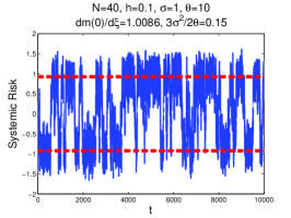
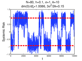
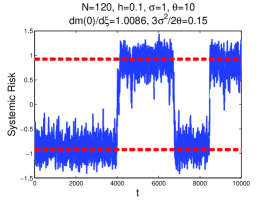
We take $U(y)=y^{3}-y$, $=1$, $X_{j}^{0}=-1$, $\Delta t=0.02$, and let $\{\Delta W_{j}^{n}\}_{j,n}$ be independent Gaussian random variables with mean zero and variance $\Delta t$. In the figures presented, the dashed lines show the numerical solutions of the compatibility equation (4), $\xi=m(\xi)$. As noted earlier, if $\frac{d}{d\xi}m(0)\leq 1$, then $0=m(0)$ is the unique solution and $0$ is a stable state. Therefore we should observe that the systemic risk fluctuates around $0$. If $\frac{d}{d\xi}m(0)>1$, there are two additional non-zero solutions $\pm\xi_{b}=m(\pm\xi_{b})$ and $\pm\xi_{b}$ are stable while $0$ is unstable. We also know that when $h$ is small, the condition $\frac{d}{d\xi}m(0)>1$ can be simplified to be $3\sigma^{2}/2\theta<1$.

Fig. 1: Simulations for different $\sigma$. The system has two (statistically) stable equilibria when $\sigma$ is below the critical value or otherwise has single stable state $0$. For small $h$, $3\sigma^{2}/2\theta<1$ is the approximate criterion.

Fig. 2: Simulations for different $\theta$. The system has two stable equilibria if $\theta$ is above the critical value or otherwise has single stable state $0$. For small $h$, $3\sigma^{2}/2\theta<1$ is the approximate criterion.

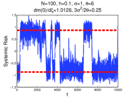
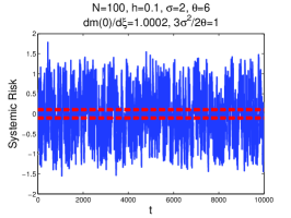
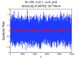
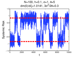
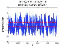
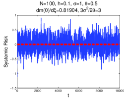
Figure 1 and Figure 2 illustrate the behavior of the empirical mean as the system transitions from having two equilibria to having a single one, which is controlled by the value of $\frac{d}{d\xi}m(0)$. This is an instance of a bifurcation of equilibria. From Proposition 2, we know that when $h$ is small, the existence condition of two equilibria, $\frac{d}{d\xi}m(0)>1$, can be approximated by the condition $3\sigma^{2}/2\theta<1$. In the simulations, we let $h=0.1$ so the approximate condition $3\sigma^{2}/2\theta<1$ can be applied. In Figure 1 we change $\sigma$ but fix the other parameters, and consider the three cases $\frac{d}{d\xi}m(0)<1$ ($3\sigma^{2}/2\theta>1$), $\frac{d}{d\xi}m(0)\approx 1$ ($3\sigma^{2}/2\theta=1$) and $\frac{d}{d\xi}m(0)>1$ ($3\sigma^{2}/2\theta<1$). In Figure 2 we change $\theta$. We can see that even though the parameters varied in the numerical simulations are not the same, the bifurcation behavior is similar.

Fig. 3: The effect of changing $h$. Increasing it stabilizes the system.

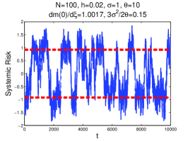
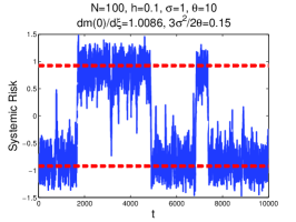
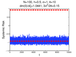
Figure 3 shows the effect of increasing $h$ on the system stability. By stability we mean resistance to the transition of the empirical mean of the system from one state to the other (because the model is symmetric). The parameter $h$ is proportional to the height of the potential barrier of each agent. Thus we increase the overall system stability if we increase the component’s stability. This observation is analogous to comments in [31, 25, 26]. It is clear that $h$ influences system stability substantially.

Fig. 4: Influence of the system size $N$. A larger system tends to have a more stable behavior.

Figure 4 illustrates the effect of system size on its stability. Clearly a larger system is more stable. These stability phenomena will be quantified with the large deviations analysis of Section 5.

4.2 Heterogeneous Model

For the heterogeneous model, $\theta$ is replaced by $\theta_{j}$, and the discretization is

$$X_{j}^{n+1}=X_{j}^{n}-hU(X_{j}^{n})\Delta t+\sigma\Delta W_{j}^{n+1}+\theta_{j}(\frac{1}{N}\sum_{k=1}^{N}X_{k}^{n}-X_{j}^{n})\Delta t,$$ (13)

with the same parameter settings. The different values of $\theta_{j}$ are controlled by the parameters $\Theta_{l}$ and $\rho_{l}$. In the simulation, we take $K=3$ and $\{\Theta_{l}\}_{l=1}^{K}=\{\Theta_{L},\Theta_{M},\Theta_{H}\}$ for a system a low, medium and high rates of mean reversion to the empirical mean, that is, the systemic risk. We also take $\{\rho_{l}\}_{l=1}^{K}=\{\rho_{L},\rho_{M},\rho_{H}\}$ for the corresponding fractions. We use the normalized standard deviation of the distribution of $\theta_{j}$ values in order to quantify diversity. We find that the heterogeneous model behaves like the homogeneous one when $h$, $\sigma$ and $N$ change. But, diversity on the rates of mean reversion has significant impact on system stability.

Fig. 5: Effect of changes in $\sigma$. The system has two stable equllibria when $\sigma$ is below the critical value and has single one otherwise. For small $h$, $\sum_{l=1}^{K}(\rho_{l}/\Theta_{l})(3\sigma^{2}/2\Theta_{l}-1)<1$ is the approximate criterion.

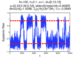
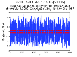
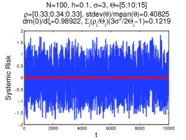
As in the homogeneous case, in Figure 5 we consider cases with $\sigma$ below, close to and above the critical value. The results are similar to the homogeneous case as expected. For $\sigma$ below the critical value we have two equlibria and for $\sigma$ above the critical value one equilibrium. The condition $\frac{d}{d\xi}m(0)>1$ is still necessary and sufficient for the existence two equlibria. The condition $\sum_{l=1}^{K}(\rho_{l}/\Theta_{l})(3\sigma^{2}/2\Theta_{l}-1)<1$ is also a good approximation to the exact one when $h$ is small.

Fig. 6: Effect of changing $h$. Increasing it stabilizes the system.

Fig. 7: Effect of changing the system size $N$. Larger system have a more stable behavior.

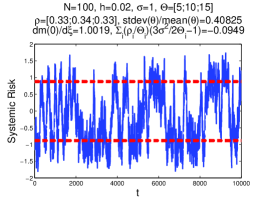
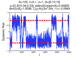
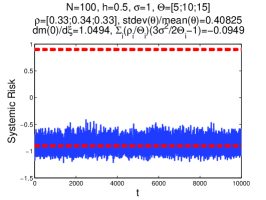
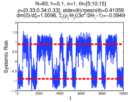
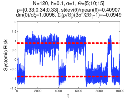
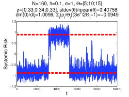
The parameter $h$ and the system size $N$ are closely associated with system stability. We note that in Figure 6 and Figure 7 when $h$ or $N$ are increased, the system becomes visibly more stable. Another observation is that with $h$, $\sigma$ and $N$ fixed, and with the mean of $\theta_{j}$ of (13) equal to $\theta$ of (12), the heterogeneous system is consistently more unstable than the corresponding homogeneous model (see Figure 3 and Figure 4). Clearly diversity tends to destabilize the system.

Fig. 8: The effect of changes in $\Theta_{l}$. The median of the diversity values is fixed but the low and high sensitivities are changed to adjust the level of diversity of $\theta_{j}$ while $\rho_{l}$ and the mean of $\theta_{j}$ are the same. Increasing diversity tends to destabilize the system.

Fig. 9: The effect of changes in $\rho_{l}$, with $\Theta_{l}$ and the mean of $\theta_{j}$ fixed. Increasing diversity tends to destabilize the system.

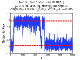
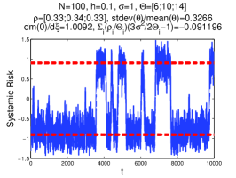
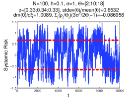
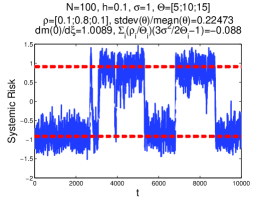
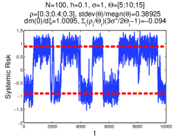
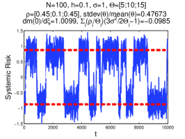
We also change the diversity of $\theta_{j}$ by changing $\Theta_{l}$ and $\rho_{l}$. To compare with the homogeneous case, in Figure 8 and Figure 9 we change the standard deviation of $\theta_{j}$ while the mean of $\theta_{j}$ is fixed. In this most interesting part of the simulations we see that when we increase the standard deviation of diversity values, the number of transitions is notably larger than that in the homogeneous case.

5 Large Deviations

In the previous two sections we saw both analytically and numerically that for large $N$, the empirical density $X_{N}(t,dy)$ is close (weakly, in probability) to the solution of the Fokker-Planck equation (2), and so the mean $\bar{x}(t)$ in (1) stays around the first order moment of the deterministic limit, $\int_{-\infty}^{\infty}yu(t,y)dy$. If the condition of existence of two equilibria is satisfied, then $\bar{x}(t)$ will remain close to either $-\xi_{b}$ or $+\xi_{b}$ for relatively long time intervals, depending in particular on the parameter $h$. However, as long as $N<\infty$, as we have seen in the simulations the random forcing by the Brownian motions $\{w_{j}(t)\}_{j=1}^{N}$ will cause transitions with non-zero probability. A systemic transition is the event that $\bar{x}(t)$ is displaced from $\pm\xi_{b}$ to $\mp\xi_{b}$ within a finite time horizon. Thus, systemic transition means that a large number of agents transition in a finite time. In this paper, we are interested in computing the probability of such a systemic transition. Mathematically, given a finite time horizon $[0,T]$ and the conditions for existence of two equilibria, we want to compute the probability

$$\mathbf{P}(\bar{x}(0)=-\xi_{b},\bar{x}(T)=\xi_{b})$$ (14)

when $N$ is large and as a function of the parameters $(h,\theta,\sigma)$ in (1).

5.1 Large Deviations of Mean-fields

According to [10], we can calculate this probability asymptotically for large $N$ using large deviations. To state the large deviations theory that we will use, we will review briefly some notation and terminology from [10].

• $M_{1}(\mathbb{R})$ is the space of probability measures on $\mathbb{R}$ with the Prohorov metric $\rho$, associated with weak convergence.

• $C([0,T],M_{1}(\mathbb{R}))$ is the space of continuous functions from $[0,T]$ to $M_{1}(\mathbb{R})$ with the metric $\sup_{0\leq t\leq T}\rho(\phi_{1}(t),\phi_{2}(t))$.

• $M_{R}(\mathbb{R})=\{\mu\in M_{1}(\mathbb{R}),\int\varphi(y)\mu(dy)\leq R\}$, where $\varphi\in C^{2}(\mathbb{R})$ is a nonnegative function with $\lim_{|x|\to\infty}\varphi(x)=\infty$. From [10], if $U(y)=y^{3}-y$, we can choose $\varphi(y)=1+y^{2}+\gamma y^{4}$, $0\leq\gamma\leq h/2$.

• $M_{\infty}(\mathbb{R})=\cup_{R>0}M_{R}(\mathbb{R})=\{\mu\in M_{1}(\mathbb{R}),\int\varphi(y)\mu(dy)<\infty\}$ endowed with the inductive topology: $\mu_{n}\rightarrow\mu$ in $M_{\infty}(\mathbb{R})$ if and only if $\mu_{n}\rightarrow\mu$ in $M_{1}(\mathbb{R})$ and $\sup_{n}\int\varphi(y)\mu_{n}(dy)<\infty$.

• $C([0,T],M_{\infty}(\mathbb{R}))$ is the space of continuous functions from $[0,T]$ to $M_{\infty}(\mathbb{R})$ endowed with the topology: $\phi_{n}(\cdot)\rightarrow\phi(\cdot)$ in $C([0,T],M_{\infty}(\mathbb{R}))$ if and only if $\phi_{n}(\cdot)\rightarrow\phi(\cdot)$ in $C([0,T],M_{1}(\mathbb{R}))$ and $\sup_{0\leq t\leq T}\sup_{n}\int\varphi(y)\phi_{n}(t,dy)<\infty$.

• Given $\nu\in M_{\infty}(\mathbb{R})$, we let $\mathcal{E}^{\nu}=\{\phi\in C([0,T],M_{\infty}(\mathbb{R})):\phi(0)=\nu\}$, endowed with the relative topology.

To simplify the notation, we rewrite (2) as $u_{t}=\mathcal{L}_{u}^{*}u+h\mathcal{M}^{*}u$, where

$$\mathcal{L}_{\psi}^{*}\phi=\frac{1}{2}\sigma^{2}\phi_{yy}+\theta\frac{\partial}{\partial y}\left\{\left[y-\int y\psi(t,y)dy\right]\phi\right\},\quad\mathcal{M}^{*}\phi=\frac{\partial}{\partial y}\left[U(y)\phi\right].$$

Theorem 7.

(Dawson and Gärtner, 1987) Given a finite horizon $\left[0,T\right]$, $\nu\in M_{\infty}(\mathbb{R})$ and $A\subseteq\mathcal{E}^{\nu}$, if $X_{N}(0)=\frac{1}{N}\sum_{j=1}^{N}\delta_{x_{j}(0)}\rightarrow\nu$ in $M_{\infty}(\mathbb{R})$ as $N\rightarrow\infty$, then the law of $X_{N}(t)=\frac{1}{N}\sum_{j=1}^{N}\delta_{x_{j}(t)}$ satisfies the large deviation principle with the good rate function $I_{h}$:

$$-\inf_{\phi\in\mathring{A}}I_{h}(\phi) \leq\liminf_{N\rightarrow\infty}\frac{1}{N}\log\mathbf{P}(X_{N}\in A)$$

$$\leq\limsup_{N\rightarrow\infty}\frac{1}{N}\log\mathbf{P}(X_{N}\in A)\leq-\inf_{\phi\in\bar{A}}I_{h}(\phi),$$

where $\mathring{A}$ and $\bar{A}$ are the interior and closure of $A$ in $\mathcal{E}^{\nu}$, respectively, and

$$I_{h}(\phi)=\frac{1}{2\sigma^{2}}\int_{0}^{T}\sup_{f:\langle\phi,f_{y}^{2}\rangle\neq 0}J_{h}(\phi,f)dt,$$ (15)

$$J_{h}(\phi,f)=\langle\phi_{t}-\mathcal{L}_{\phi}^{*}\phi-h\mathcal{M}^{*}\phi,f\rangle^{2}/\langle\phi,f_{y}^{2}\rangle,\quad\langle\phi,f\rangle=\int_{-\infty}^{\infty}f(y)\phi(dy),$$

if $\phi(t)$ is absolutely continuous in $t\in[0,T]$ and $I_{h}(\phi)=\infty$ otherwise.

Remark. Here for $\phi\in{\cal E}^{\nu}$ and $t\in[0,T]$, $\phi(t)$ is viewed as a real Schwartz distribution on $\mathbb{R}$, $\mathcal{L}_{\psi}^{*}$ and $\mathcal{M}^{*}\phi$ are differential operators in the distribution sense, and $f$ in (15) is a real Schwartz test function. The definition of absolute continuity for the path of measures $(\phi(t))_{t\in[0,T]}$ is in the sense of Definition 4.1 in [10], that is to say: for each compact set $K\subset\mathbb{R}$ there exists a neighborhood $U_{K}$ of the null function in the set of test functions with compact support in $K$ and an absolutely continuous function $H_{K}$ from $[0,T]$ to $\mathbb{R}$ such that $|\langle\phi(t),f\rangle-\langle\phi(s),f\rangle|\leq|H_{K}(t)-H_{K}(s)|$ for all $s,t\in[0,T]$ and $f\in U_{K}$. Note that by Lemma 4.2 in [10], if $\phi(t)$ is absolutely continuous in $t\in[0,T]$, $\phi_{t}(t)$ exists in the distribution sense almost everywhere on $t\in[0,T]$.

In order to use Theorem 7, we let $\nu=u^{e}_{-\xi_{b}}$ in (3) and define the rare event $A$ of systemic transition by

$$A=\left\{\phi\in\mathcal{E}^{\nu}:\phi(T)=u^{e}_{\xi_{b}}\right\}.$$ (16)

However, since $\mathring{A}$ is an empty set, Theorem 7 give a trivial lower bound for the probability in question. Therefore we consider instead the closed rare event $A_{\delta}$:

$$A_{\delta}=\left\{\phi\in\mathcal{E}^{\nu}:\rho(\phi(T),u^{e}_{\xi_{b}})\leq\delta\right\}.$$

Then Theorem 7 implies that

$$-\inf_{\phi\in\mathring{A}_{\delta}}I_{h}(\phi) \leq\liminf_{N\rightarrow\infty}\frac{1}{N}\log\mathbf{P}(X_{N}\in A_{\delta})$$

$$\leq\limsup_{N\rightarrow\infty}\frac{1}{N}\log\mathbf{P}(X_{N}\in A_{\delta})\leq-\inf_{\phi\in A_{\delta}}I_{h}(\phi).$$

In addition, we show that $\inf_{\phi\in A_{\delta}}I_{h}(\phi)$ can be bounded from below by $\inf_{\phi\in A}I_{h}(\phi)$ as $\delta\rightarrow 0$.

Lemma 8.

By definition $\inf_{\phi\in A_{\delta}}I_{h}(\phi)$ is decreasing with $\delta>0$ and bounded from above by $\inf_{\phi\in A}I_{h}(\phi)$. In addition,

$$\lim_{\delta\to 0}\inf_{\phi\in A_{\delta}}I_{h}(\phi)\geq\inf_{\phi\in A}I_{h}(\phi).$$

Proof.

See Appendix C. ∎

Combining Lemma 8 and the fact that $\inf_{\phi\in\mathring{A}_{\delta}}I_{h}(\phi)\leq\inf_{\phi\in A}I_{h}(\phi)$, for any $\epsilon>0$, we have for sufficiently small $\delta>0$

$$-\inf_{\phi\in A}I_{h}(\phi) \leq\liminf_{N\rightarrow\infty}\frac{1}{N}\log\mathbf{P}(X_{N}\in A_{\delta})$$

$$\leq\limsup_{N\rightarrow\infty}\frac{1}{N}\log\mathbf{P}(X_{N}\in A_{\delta})\leq-\inf_{\phi\in A}I_{h}(\phi)+\epsilon.$$

Therefore for large $N$ and sufficiently small $\delta$,

$$\mathbf{P}(X_{N}\in A_{\delta})\approx\exp\left(-N\inf_{\phi\in A}I_{h}(\phi)\right).$$ (17)

This tells us that a larger system has a more stable empirical mean trajectory, which is consistent with what we have seen in the numerical simulation. Now the main step is finding $\inf_{\phi\in A}I_{h}(\phi)$, which is a min-max variational problem

$$\inf_{\phi\in A}I_{h}(\phi)=\inf_{\phi\in A}\frac{1}{2\sigma^{2}}\int_{0}^{T}\sup_{f:\langle\phi,f_{y}^{2}\rangle\neq 0}\langle\phi_{t}-\mathcal{L}_{\phi}^{*}\phi-h\mathcal{M}^{*}\phi,f\rangle^{2}/\langle\phi,f_{y}^{2}\rangle dt,$$ (18)

where the $f$ in the $\sup$ is a real Schwartz test function.

5.2 An Alternative Expression for the Rate Function

The representation of the rate function (15) is somewhat complicated, but we can simplify it if $\phi$ has the density with some additional properties. If $\phi$ is a density function such that $\phi(t,y)$ is smooth, rapidly decreasing in $y\in\mathbb{R}$ for each $t\in[0,T]$ and is absolutely continuous in $t\in[0,T]$ for each $y\in\mathbb{R}$, then let $g(t,y)$ satisfy

$$\phi_{t}-\mathcal{L}_{\phi}^{*}\phi-h\mathcal{M}^{*}\phi=(\phi g)_{y}.$$ (19)

Note that because of the properties of $\phi$, the left hand side of (19) is well-defined in $y\in\mathbb{R}$ and almost everywhere in $t\in[0,T]$. In addition, because $\phi$ is positive valued, $g$ exists and is unique except on a measure zero set in $[0,T]$.

Note that for the pair $(\phi,g)$ satisfying (19)

$$\sup_{f:\langle\phi(t),f_{y}^{2}\rangle\neq 0}J_{h}(\phi(t),f)=\sup_{f:\langle\phi(t),f_{y}^{2}\rangle\neq 0}\langle\phi(t),f_{y}g\rangle^{2}/\langle\phi(t),f_{y}^{2}\rangle=\langle\phi(t),g^{2}\rangle,$$

and therefore we have the following proposition.

Proposition 9.

If $\phi$ is a density function such that $\phi(t)$ is a Schwartz function for each $t\in[0,T]$ and is absolutely continuous in $t\in[0,T]$ for each $y\in\mathbb{R}$, and $g(t,y)$ satisfies (19), the rate function $I_{h}(\phi)$ in (15) can be written in the form

$$I_{h}(\phi)=\frac{1}{2\sigma^{2}}\int_{0}^{T}\langle\phi,g^{2}\rangle dt.$$ (20)

We interpret (19) and (20) as follows. The function $g$ is regarded as the driving force making $\phi$ deviate from the solution of the Fokker-Planck equation (2), and $I_{h}(\phi)$ is the $L^{2}(\phi)$ norm of $g$, which measures how difficult it is to have this deviation $\phi$.

6 Small $h$ Analysis

The goal of this section is to analyze the min-max problem (18) which controls the asymptotic systemic transition probability. This problem is nonlinear and infinitely dimensional and is difficult to analyze. To get some useful information about it we will assume that $h$ is small and analyze it in this regime. We will first solve (18) when $h$ is exactly $0$, and then we will get rigorous upper and lower bounds for (18) when $h$ is nonzero but small. We will then compare the large deviations result with the local fluctuation theory of a single agent so as to explain why interconnectedness destabilizes the system.

6.1 The $h=0$ and the Small $h$ Analysis

We note that when $h=0$, $u_{\pm\xi_{b}}^{e}=u_{\pm\xi_{0}}^{e}$, where

$$u_{\pm\xi_{0}}^{e}(y)=\frac{1}{\sqrt{2\pi\frac{\sigma^{2}}{2\theta}}}\exp\left\{-\frac{(y-(\pm\xi_{0}))^{2}}{2\frac{\sigma^{2}}{2\theta}}\right\},\quad\quad\xi_{0}=\sqrt{1-3\frac{\sigma^{2}}{2\theta}}.$$ (21)

In this case, (18) is solvable and the optimal path is a Gaussian, starting from $u_{-\xi_{0}}^{e}$ and ending in $u_{+\xi_{0}}^{e}$.

Theorem 10.

Let $h=0$ and define

$$p^{e}(t,y)=\frac{1}{\sqrt{2\pi\frac{\sigma^{2}}{2\theta}}}\exp\left\{-\frac{(y-a^{e}(t))^{2}}{2\frac{\sigma^{2}}{2\theta}}\right\},\quad a^{e}(t)=\frac{2\xi_{0}}{T}t-\xi_{0}.$$ (22)

Then $p^{e}\in A$ is the unique minimizer for (18) and

$$\inf_{\phi\in A}I_{0}(\phi)=I_{0}(p^{e})=\frac{2\xi_{0}^{2}}{\sigma^{2}T}.$$

Proof.

See Appendix D.1. ∎

We show next that (18) is continuous at $h=0$.

Theorem 11.

There exists $\gamma(h)$ such that $\gamma(h)\to 0$ as $h\to 0$ and

$$\Big{|}\inf_{\phi\in A}I_{h}(\phi)-\frac{2\xi_{b}^{2}}{\sigma^{2}T}\Big{|}\leq\gamma(h).$$ (23)

We recall here that

$$\xi_{b}=\xi_{0}+h\xi_{1}+O(h^{2}),\quad\quad\xi_{1}=\sqrt{1-3\frac{\sigma^{2}}{2\theta}}\frac{6}{\sigma^{2}}\left(\frac{\sigma^{2}}{2\theta}\right)^{2}\frac{1-2(\sigma^{2}/2\theta)}{1-3(\sigma^{2}/2\theta)}.$$ (24)

Proof.

See Appendix D.2 and D.3. ∎

As it is stated we could replace $\xi_{b}$ by $\xi_{0}$ in Theorem 11, since $\xi_{b}=\xi_{0}+o(1)$ as $h\to 0$. We will see in the next section (in Proposition 19) that $\gamma(h)=O(h^{2})$. In fact we show this rigorously for the upper bound but only formally for the lower bound. Since $\xi_{b}=\xi_{0}+h\xi_{1}+O(h^{2})$ we see that the term $2\xi_{b}^{2}/(\sigma^{2}T)$ contains the leading-order term and the first-order correction in the $h$-expansion of $\inf_{\phi\in A}I_{h}(\phi)$.

6.2 Large Deviations for the First Exit Time

In this subsection, we consider the rare event $B$ of systemic transition at some time before $T$:

$$B_{\delta}=\{\phi\in\mathcal{E}^{\nu}:\exists t\in(0,T],\rho(\phi(t),u^{e}_{\xi_{b}})\leq\delta\}.$$

In other words, $B_{\delta}=\cup_{t\in(0,T]}A_{\delta}(t)$, where

$$A_{\delta}(t)=\{\phi\in\mathcal{E}^{\nu}:\rho(\phi(t),u^{e}_{\xi_{b}})\leq\delta\}.$$

We let $B:=B_{0}$. We then have that

Lemma 12.

By definition $\inf_{\phi\in B_{\delta}}I_{h}(\phi)$ is decreasing with $\delta>0$ and bounded from above by $\inf_{\phi\in B}I_{h}(\phi)$. In addition,

$$\lim_{\delta\to 0}\inf_{\phi\in B_{\delta}}I_{h}(\phi)=\inf_{\phi\in\cup_{t\in(0,T]}A(t)}I_{h}(\phi)=\inf_{\phi\in B}I_{h}(\phi),$$

where $A(t):=A_{0}(t)$.

Proof.

See Appendix D.4. ∎

From Theorem 11, we see that in the sense of large deviations the probability of system failure at some time before time $T$ is essentially the same as the probability of system failure at time $T$.

Corollary 13.

For any $t_{1}<t_{2}$, there exists a sufficiently small $h$ such that $\inf_{\phi\in A(t_{1})}I_{h}(\phi)>\inf_{\phi\in A(t_{2})}I_{h}(\phi)$. Consequently, $\inf_{\phi\in B}I_{h}(\phi)\approx\inf_{\phi\in A(T)}I_{h}(\phi)$ for small $h$.

6.3 Comparison with the Fluctuation Theory of a Single Agent

To get a better understanding of the large deviations results we need to carry out a standard fluctuation theory for a single agent. We assume that $x_{j}(0)=-1$ for all $j$ and that the $x_{j}(t)$’s are in the vicinity of $-1$ so that we can linearize (1):

$$x_{j}(t)=-1+z_{j}(t),\quad\bar{x}(t)=-1+\bar{z}(t),\quad\bar{z}(t)=\frac{1}{N}\sum_{j=1}^{N}z_{j}(t).$$

For $V(y)=\frac{1}{4}y^{4}-\frac{1}{2}y^{2}$, $z_{j}(t)$ and $\bar{z}(t)$ satisfy the linear stochastic differential equations

$$dz_{j}=-(\theta+2h)z_{j}dt+\theta\bar{z}dt+\sigma dw_{j},\quad d\bar{z}=-2h\bar{z}dt+\frac{\sigma}{N}\sum_{j=1}^{N}dw_{j},$$

with $z_{j}(0)=\bar{z}(0)=0$. The processes $z_{j}(t)$ and $\bar{z}(t)$ are Gaussian and the mean and variance functions are easily calculated. We are especially interested in their behavior for large $N$.

Lemma 14.

For all $t\geq 0$, $\mathbf{E}z_{j}(t)=\mathbf{E}\bar{z}(t)=0$ and $\mathbf{Var}\bar{z}(t)=\frac{\sigma^{2}}{N}(1-e^{-4ht})$. In addition, $\mathbf{Var}z_{j}(t)\rightarrow\frac{\sigma^{2}}{2(\theta+2h)}(1-e^{-2(\theta+2h)t})$ as $N\rightarrow\infty$, uniformly in $t\geq 0$.

From Lemma 14, we see that $\sigma^{2}/N$ and $\sigma^{2}/2(\theta+2h)$ should be sufficiently small so that linearization is consistent with the results it produces.

6.4 Increased Probability of Large Deviations for Increased $\theta$ and Its Systemic Risk Interpretation

We have now the analytical results with which we may conclude that individual risk diversification may increase the systemic risk. Assume that $\sigma^{2}/N$ and $\sigma^{2}/2(\theta+2h)$ are sufficiently small and $N$ is large. From Lemma 14, the risk $x_{j}(t)$ of the agent $j$ is approximately a Gaussian process with the stationary distribution $\mathcal{N}(-1,\sigma^{2}/2(\theta+2h))$. If the external risk, $\sigma$ is high, then in order to keep the risk $x_{j}(t)$ at an acceptable level, the agent may increase the intrinsic stability, $h$, or share the risk with other agents, that is, increase $\theta$. Increasing $h$ is in general more costly (cuts into profits) than increasing $\theta$, and at the individual agent level there is no difference in risk assessment between increasing $h$ and increasing $\theta$. Therefore the agents are likely to increase $\theta$ and reduce individual risk by diversifying it. Note that $\sigma^{2}/2(\theta+2h)\lesssim\sigma^{2}/2\theta$ when $\sigma^{2}$ and $\theta$ are significantly larger than $h$. Thus, individual agents can maintain low locally assessed risk by diversification, even in a very uncertain environment.

What is not perceived by the individual agents, however, is that risk diversification may increases the systemic risk while it reduces their individual risk. Because $\sigma^{2}$ and $\theta$ are significantly larger than $h$, the small $h$ analysis can be applied and from (17) and Theorem 11, the systemic risk (the probability of the system failure) is

$$\mathbf{P}(X_{N}\in B_{\delta})\approx\exp\left(-N\frac{2\xi_{b}^{2}}{\sigma^{2}T}\right),\quad\text{for small $\delta$ and $h$,}$$

$$\xi_{b}=\sqrt{1-3\frac{\sigma^{2}}{2\theta}}\left(1+h\frac{6}{\sigma^{2}}\left(\frac{\sigma^{2}}{2\theta}\right)^{2}\frac{1-2(\sigma^{2}/2\theta)}{1-3(\sigma^{2}/2\theta)}\right)+O(h^{2}).$$

We see that there are additional systemic-level $\sigma^{2}$ terms in the exponent and $\xi_{b}$, which can not be observed by the agents, increasing the systemic risk, even if the individual risk $\sigma^{2}/2\theta$ is fixed. In other words, the individual agents may believe that they are able to withstand larger external fluctuations as long as their risk can be diversified, but a higher $\sigma$ tends to destabilize the system.

7 A Reduced Large Deviations Principle for Small $h$

In Section 6.1, we show that the large deviation problem $\inf_{\phi\in A}I_{h}(\phi)$ is continuous in $h$ so that we have the upper and lower bounds for $\inf_{\phi\in A}I_{h}(\phi)$ when $h$ is small. In this section, we analyze with a formal expansion the optimal path for $\inf_{\phi\in A}I_{h}(\phi)$ by assuming that it is of the form $p^{e}+O(h)$, motivated by the fact that the optimal path is $p^{e}$ for $h=0$. In this way, we can obtain a reduced large deviations principle (a reduced Freidlin-Wentzell theory) for the systemic risk. That is, we obtain a reduced rate function corresponding to a finite dimensional system after ignoring higher order terms. The reduced rate function has all relevant information up to $O(h^{2})$ terms, and we also need to expand $\phi$ to $O(h^{2})$.

We assume that the optimal $\phi=p+hq^{(1)}+h^{2}q^{(2)}+\ldots$, where

$$p(t,y)=\frac{1}{\sqrt{2\pi\frac{\sigma^{2}}{2\theta}}}\exp\left\{-\frac{(y-a(t))^{2}}{2\frac{\sigma^{2}}{2\theta}}\right\},\quad a(t)=\langle\phi,y\rangle.$$

In other words, we let the first moment of $\phi$ be determined by $a(t)$, and from the zero $h$ case we know that $a(t)=a^{e}(t)+O(h)$. From the form of $p$ and (19), a natural parameterization for $q^{(1)}$ and $q^{(2)}$ is the Hermite expansion

$$q^{(1)}(t,y)=\sum_{n=2}^{\infty}b_{n}(t)\frac{\partial^{n}}{\partial y^{n}}p(t,y),\quad q^{(2)}(t,y)=\sum_{n=2}^{\infty}c_{n}(t)\frac{\partial^{n}}{\partial y^{n}}p(t,y).$$

Note that by the properties of $p$ and $a(t)$, $\langle q^{(1)},y^{n}\rangle=\langle q^{(2)},y^{n}\rangle=0$ for $n=0,1$ so we can start the Hermite expansion from $n=2$.

The formal expansion result of this section is that if the optimal $\phi=p+hq^{(1)}+h^{2}q^{(2)}$, then

$$\inf_{\phi\in A}I_{h}(\phi)\approx\inf_{\begin{subarray}{c}a(t):0\leq t\leq T\\ a(0)=-\xi_{b}\\ a(T)=\xi_{b}\end{subarray}}\frac{1}{2\sigma^{2}}\int_{0}^{T}\left(\frac{d}{dt}a+h(a^{3}+3\frac{\sigma^{2}}{2\theta}a-a)\right)^{2}dt,$$ (25)

for small $h$. Note that $a(t)=\langle\phi,y\rangle=\bar{x}(t)$. The right hand side of (25) is an one-dimensional variational problem that has the form of a rate function of the Freidlin-Wentzell theory. In fact, the right side of (25) is the large deviations variational problem for the rate function of the small-noise stochastic differential equation

$$d\bar{x}(t)=-h\left[\bar{x}^{3}(t)-\left(1-\frac{3\sigma^{2}}{2\theta}\right)\bar{x}(t)\right]dt+\epsilon\sigma dw(t)$$ (26)

where here $\epsilon=1/\sqrt{N}$ is small. Note that ${3\sigma^{2}}/{2\theta}<1$, as assumed above, and therefore (26) also represents a bi-stable structure. In the remainder of this section we describe how this result is obtained by formal expansions and then in Section 7.3 we show how we recover from (25) the main result of the paper stated in the previous section.

An important remark about the expansion is that the Hermite functions are a basis of the $L^{2}$ space and thus $p+hq^{(1)}+h^{2}q^{(2)}$ is generally a signed measure. However, if $q^{(1)}$ and $q^{(2)}$ can be expressed as the linear combinations of finite Hermite functions, then we can see that for any $\epsilon>0$, there exists a sufficiently small $h$ such that the negative part of $p+hq^{(1)}+h^{2}q^{(2)}$ is less than $\epsilon$.

7.1 Optimization over $g$

The first step in finding the optimal $\phi=p+hq^{(1)}+h^{2}q^{(2)}$ is determining the optimal $g$ by using (19) for $\phi$. Once we obtain $g$, we can compute $I_{h}(\phi)$ by using (20). It is also natural to assume that $g=g^{(0)}+hg^{(1)}+h^{2}g^{(2)}$ along with the Hermite expansion:

$$g^{(0)}=p^{-1}\sum_{n=0}^{\infty}\alpha_{n}(t)\frac{\partial^{n}}{\partial y^{n}}p,\quad g^{(1)}=p^{-1}\sum_{n=0}^{\infty}\beta_{n}(t)\frac{\partial^{n}}{\partial y^{n}}p,\quad g^{(2)}=p^{-1}\sum_{n=0}^{\infty}\gamma_{n}(t)\frac{\partial^{n}}{\partial y^{n}}p.$$

In addition, since $\langle q^{(1)},y\rangle=\langle q^{(2)},y\rangle=0$, we can see that $\phi=p+hq^{(1)}+h^{2}q^{(2)}$ satisfies

$$\mathcal{L}_{\phi}^{*}\phi=\mathcal{L}_{p}^{*}p+h\mathcal{L}_{p}^{*}q^{(1)}+h^{2}\mathcal{L}_{p}^{*}q^{(2)},\quad\mathcal{M}^{*}\phi=\mathcal{M}^{*}p+h\mathcal{M}^{*}q^{(1)}+h^{2}\mathcal{M}^{*}q^{(2)}.$$

The force $U(y)=y^{3}-y$ can also be expanded in Hermite polynomials:

$$U(y)=p^{-1}\sum_{n=0}^{3}\delta_{n}(t)\frac{\partial^{n}}{\partial y^{n}}p.$$

Now everything is expanded in the orthogonal basis and we can find the optimal $g^{(0)}$ and $g^{(1)}$ by putting everything into (19) and comparing coefficients.

Lemma 15.

With the expansions mentioned above, the optimal $g^{(0)}$ is $-\frac{d}{dt}a$, and the optimal $\beta_{n}$ for $g^{(1)}$ are

$$\beta_{n}=\begin{cases}-\delta_{0}=-\langle p,U(y)\rangle,&n=0,\\ \frac{d}{dt}b_{n+1}+\theta(n+1)b_{n+1}-\delta_{n},&1\leq n\leq 3,\\ \frac{d}{dt}b_{n+1}+\theta(n+1)b_{n+1},&n\geq 4.\end{cases}$$ (27)

Proof.

See Appendix E.1. ∎

It remains to determine $g^{(2)}$. From (20) we see that the only contribution of $g^{(2)}$ to $I_{h}$ up to $O(h^{2})$ is $\langle p,2g^{(0)}g^{(2)}\rangle=-2\gamma_{0}\frac{d}{dt}a$. Thus it suffices to determine $\gamma_{0}$, which can also be obtained from (19).

Lemma 16.

With the expansions mentioned above, the optimal $\gamma_{0}$ is

$$\gamma_{0}=-\langle q^{(1)},U(y)+g^{(1)}\rangle.$$

Proof.

See Appendix E.2. ∎

7.2 Optimization over $\phi$

We are now ready to find the optimal $\phi$. For given $\phi=p+hq^{(1)}+h^{2}q^{(2)}$ and the corresponding optimal $g=g^{(0)}+hg^{(1)}+h^{2}g^{(2)}$, (20) gives

$$I_{h}(\phi) =\frac{1}{2\sigma^{2}}\int_{0}^{T}\langle p+hq^{(1)}+h^{2}q^{(2)},(g^{(0)}+hg^{(1)}+h^{2}g^{(2)})^{2}\rangle dt$$

$$=\frac{1}{2\sigma^{2}}\int_{0}^{T}\langle p,(g^{(0)})^{2}\rangle dt+\frac{h}{2\sigma^{2}}\int_{0}^{T}\langle p,2g^{(0)}g^{(1)}\rangle dt$$

$$\quad+\frac{h^{2}}{2\sigma^{2}}\int_{0}^{T}\left(\langle p,(g^{(1)})^{2}+2g^{(0)}g^{(2)}\rangle+\langle q^{(1)},2g^{(0)}g^{(1)}\rangle\right)dt+O(h^{3}).$$

From Lemma 16, $\langle p,2g^{(0)}g^{(2)}\rangle=-2g^{(0)}\langle q^{(1)},U(y)+g^{(1)}\rangle$, and therefore

$$\langle p,2g^{(0)}g^{(2)}\rangle+\langle q^{(1)},2g^{(0)}g^{(1)}\rangle=-2g^{(0)}\langle q^{(1)},U(y)\rangle=-2g^{(0)}\sum_{n=2}^{3}H_{n}\delta_{n}b_{n},$$

where $H_{n}(t):=\langle p^{-1},(\partial^{n}p/\partial y^{n})^{2}\rangle$. We note that

$$\langle p,2g^{(0)}g^{(1)}\rangle=-2g^{(0)}\delta_{0},\quad\langle p,(g^{(1)})^{2}\rangle=\delta_{0}^{2}+\sum_{n=1}^{\infty}H_{n}\beta_{n}^{2},\quad\langle p,(g^{(0)})^{2}\rangle=(g^{(0)})^{2}.$$

Then $I_{h}(\phi)$ can be written as

$$I_{h}(\phi) =\frac{1}{2\sigma^{2}}\int_{0}^{T}(g^{(0)}-h\delta_{0})^{2}dt+\frac{h^{2}}{2\sigma^{2}}\int_{0}^{T}(H_{1}\beta_{1}^{2}-2H_{2}g^{(0)}\delta_{2}b_{2})dt$$ (28)

$$\quad+\frac{h^{2}}{2\sigma^{2}}\int_{0}^{T}(H_{2}\beta_{2}^{2}-2H_{3}g^{(0)}\delta_{3}b_{3})dt+\frac{h^{2}}{2\sigma^{2}}\sum_{n=3}^{\infty}\int_{0}^{T}H_{n}\beta_{n}^{2}dt+O(h^{3}).$$

We see that $a$ and $b_{n}$ are coupled at the $O(h^{2})$ level of (28). However, from the results of the zero $h$ case, $a=a^{e}+O(h)$ and $p=p^{e}+O(h)$ so we can decouple $a$ and $b_{n}$ and express the expanded $I_{h}(\phi)$ up to $O(h^{2})$ as the sum of independent terms.

Proposition 17.

To order $O(h^{2})$, the rate function $I_{h}(\phi)$ can be written as the sum of independent terms:

$$I_{h}(\phi) =\frac{1}{2\sigma^{2}}\int_{0}^{T}(g^{(0)}-h\delta_{0})^{2}dt+\frac{h^{2}}{2\sigma^{2}}\int_{0}^{T}(\tilde{H}_{1}\tilde{\beta}_{1}^{2}+2\frac{d}{dt}a^{e}\tilde{H}_{2}\tilde{\delta}_{2}b_{2})dt$$ (29)

$$\quad+\frac{h^{2}}{2\sigma^{2}}\int_{0}^{T}(\tilde{H}_{2}\tilde{\beta}_{2}^{2}+2\frac{d}{dt}a^{e}\tilde{H}_{3}\tilde{\delta}_{3}b_{3})dt+\frac{h^{2}}{2\sigma^{2}}\sum_{n=3}^{\infty}\int_{0}^{T}\tilde{H}_{n}\tilde{\beta}_{n}^{2}dt+O(h^{3}),$$

where $\tilde{H}_{n}(t)=\langle(p^{e})^{-1},(\partial^{n}p^{e}/\partial y^{n})^{2}\rangle$, $U(y)=(p^{e})^{-1}\sum_{n=0}^{3}\tilde{\delta}_{n}(t)\frac{\partial^{n}}{\partial y^{n}}p^{e}$, and

$$\tilde{\beta}_{n}=\begin{cases}-\tilde{\delta}_{0}=-\langle p^{e},U(y)\rangle,&n=0,\\ \frac{d}{dt}b_{n+1}+\theta(n+1)b_{n+1}-\tilde{\delta}_{n},&1\leq n\leq 3,\\ \frac{d}{dt}b_{n+1}+\theta(n+1)b_{n+1},&n\geq 4.\end{cases}$$ (30)

We can see from (29) that $q^{(2)}$ does not appear in terms up to $O(h^{2})$. From the $h$ expansion of $u^{e}_{\pm\xi_{b}}$ in (3), and the fact that $V(y)$ is a polynomial of degree four, we have $b_{n+1}(0)=b_{n+1}(T)=0$ for $n\geq 4$. The variational problem for $b_{n+1}$ is to minimize $\int_{0}^{T}\tilde{H}_{n}\tilde{\beta}_{n}^{2}dt$ where $\tilde{\beta}_{n}$ is given in terms of $b_{n+1}$ by (30). The obvious solution of this problem is $b_{n+1}=0$ and $\tilde{\beta}_{n}=0$ for $n\geq 4$. Consequently, in order to find the optimal $\phi$ for $I_{h}(\phi)$ in (29), we may solve separately the variational problems for $a$, $b_{1}$, $b_{2}$ and $b_{3}$.

7.3 Probability of Systemic Transitions for Small $h$

We consider the small probability of systemic transitions for large $N$ and small $h$ through the large deviation $\inf_{\phi\in A}I_{h}(\phi)$. Here we consider the solution up to $O(h)$ terms. That is, using (29), we solve the variational problem for $a(t)$:

$$\inf_{\begin{subarray}{c}a(t):0\leq t\leq T\\ a(0)=-\xi_{b}\\ a(T)=\xi_{b}\end{subarray}}\int_{0}^{T}(g^{(0)}-h\delta_{0})^{2}dt=\inf_{\begin{subarray}{c}a(t):0\leq t\leq T\\ a(0)=-\xi_{b}\\ a(T)=\xi_{b}\end{subarray}}\int_{0}^{T}(\frac{d}{dt}a+h(a^{3}+3\frac{\sigma^{2}}{2\theta}a-a))^{2}dt.$$ (31)

By simple calculus of variations methods we find the optimal $a$.

Lemma 18.

The optimal $a(t)$ for (31) satisfies the second order ordinary differential equation

$$\frac{d^{2}}{dt^{2}}a=h^{2}(a^{3}+(3\frac{\sigma^{2}}{2\theta}-1)a)(3a^{2}+(3\frac{\sigma^{2}}{2\theta}-1))$$

with $a(0)=-\xi_{b}$ and $a(T)=\xi_{b}$. Consequently, the optimal path is

$$a(t)=\frac{2\xi_{b}}{T}t-\xi_{b}+O(h^{2}).$$ (32)

By inserting (32) into (31) we obtain $\inf_{\phi\in A}I_{h}(\phi)$ up to $O(h)$.

Proposition 19.

For small $h$, the large deviations problem, $\inf_{\phi\in A}I_{h}(\phi)$, up to $O(h)$, is

$$\inf_{\phi\in A}I_{h}(\phi)=\frac{2\xi_{0}}{\sigma^{2}T}(\xi_{0}+2h\xi_{1})+O(h^{2}),$$ (33)

where $\xi_{b}=\xi_{0}+h\xi_{1}+O(h^{2})$ from (6). Note that $\xi_{1}$ is positive because $2\theta>3\sigma^{2}$.

Proof.

See Appendix E.3. ∎

The asymptotic probability of systemic transition for large $N$ and sufficiently small $\delta$ and $h$ has the form

$$\mathbf{P}(X_{N}\in A_{\delta})\approx\exp\left(-N\inf_{\phi\in A}I_{h}(\phi)\right)=\exp\left(-N\left\{\frac{2\xi_{0}}{\sigma^{2}T}(\xi_{0}+2h\xi_{1})+O(h^{2})\right\}\right).$$

8 Effect of Diversity of Sensitivities on the Transition Probability

We consider the situation introduced in Section 3 and analyze it when $h=0$. We aim at computing the transition probability in this situation. The $K$ partial empirical averages

$$\bar{x}_{k}(t):=\frac{1}{|\mathcal{I}_{k}|}\sum_{j\in\mathcal{I}_{k}}x_{j}(t),\quad k=1,\ldots,K$$ (34)

then satisfy a closed system of stochastic differential equations

$$d\bar{x}_{k}=\frac{\sigma}{\sqrt{\rho_{k}N}}d\bar{w}_{k}(t)-\theta_{k}(\bar{x}_{k}-\bar{x})dt$$ (35)

where $\bar{w}_{k}$ are independent Brownian motions and the empirical mean $\bar{x}(t)$ can be expressed in terms of the partial averages as

$$\bar{x}(t)=\sum_{k=1}^{K}\rho_{k}\bar{x}_{k}(t)$$

Proposition 20.

If $\bar{x}_{k}(0)=-\xi_{b}$ for all $k=1,\ldots,K$, then $\bar{x}(T)$ is a Gaussian random variable with mean $-\xi_{b}$ and variance $\sigma_{T}^{2}:={\rm Var}(\bar{x}(T))$ given by

$$\sigma_{T}^{2}=\frac{\sigma^{2}}{N}\int_{0}^{T}\varrho^{\mathbf{T}}e^{Ms}R^{-1}(e^{Ms})^{\mathbf{T}}\varrho ds$$ (36)

where $\varrho$ is the $K$-dimensional column vector $(\rho_{k})_{k=1,\ldots,K}$, $M$ and $R$ are the $K\times K$ matrices defined by

$$M_{ij}=-\theta_{i}(\delta_{ij}-\rho_{j}),\quad\quad R_{ij}=\rho_{i}\delta_{ij},\quad\quad i,j=1,\ldots,K,$$

and ^T stands for the transpose.

Proof.

See Appendix F.1. ∎

We can then deduce that the transition probability is

$$p_{T}\approx\exp\Big{(}-\frac{2\xi_{b}^{2}}{\sigma_{T}^{2}}\Big{)}$$ (37)

Our next goal is to study the impact of the diversity on the transition probability.

Proposition 21.

Let us assume that the diversity is small:

$$\theta_{k}=\bar{\theta}(1+\delta\alpha_{k}),\quad\quad\delta\ll 1$$

where $\sum_{k}\rho_{k}\alpha_{k}=0$ so that $\bar{\theta}$ is the mean value of the $\theta_{k}$’s. The equilibrium position $\xi_{b}$, the variance $\sigma_{T}^{2}$ and the transition probability $p_{T}$ can be expanded as powers of $\delta$ as

$$\xi_{b}^{2} =\Big{(}1-\frac{3\sigma^{2}}{2\bar{\theta}}\Big{)}-\delta^{2}\Big{(}\sum_{k}\rho_{k}\alpha_{k}^{2}\Big{)}\frac{3\sigma^{2}}{2\bar{\theta}}+O(\delta^{3}),$$

$$\sigma_{T}^{2} =\frac{\sigma^{2}T}{N}\Big{[}1+\delta^{2}\Big{(}\sum_{k}\rho_{k}\alpha_{k}^{2}\Big{)}\Big{(}\frac{1}{T}\int_{0}^{T}(1-e^{-\bar{\theta}s})^{2}ds\Big{)}+O(\delta^{3})\Big{]},$$

$$p_{T} \approx\exp\Big{\{}-\frac{2N}{\sigma^{2}T}\Big{[}\Big{(}1-\frac{3\sigma^{2}}{2\bar{\theta}}\Big{)}-\delta^{2}\Big{(}\sum_{k}\rho_{k}\alpha_{k}^{2}\Big{)}\Big{(}\frac{3\sigma^{2}}{2\bar{\theta}}+\frac{1}{T}\int_{0}^{T}(1-e^{-\bar{\theta}s})^{2}ds\Big{)}\Big{]}\Big{\}}.$$

Proof.

See Appendix F.2. ∎

This proposition shows that the diversity reduces the gap between the two equilibrium states and enhances the fluctuations of the empirical mean. Both effects contribute to the increase of the systemic transition probability.

9 Summary and Conclusions

The aim of this paper is to introduce and analyze a mathematical model for the evolution of risk in a system of interacting agents where cooperation between them can reduce their individual risk of failure but increase the systemic or overall risk. The model we use is a system of bistable diffusion processes that interact through their empirical mean, a mean field model. We take the rate of mean reversion to the empirical mean $\theta$ as a measure of cooperation, the depth of the bistable potential $h$ as a measure of intrinsic stability of each agent, and the strength of the external random perturbations $\sigma$ as the level of uncertainty in which the agents function. Using the theory of large deviations we calculate the probability that the system will transition from one of the two bistable states to the other during a time interval of length $T$, when the number of agents $N$ is large and when $h$ is small. In this regime of parameters we find that systemic risk increases with cooperation. The formula from which we draw this conclusion is given is Section 6.4. We also show that when the rate of mean reversion to the empirical mean varies among the different agents, that is, when there is diversity in the cooperative behavior then the probability of transitions increases, which means that the systemic risk increases.

Appendix A Proof of Proposition 2

For small $h$, we view $u^{e}_{\xi}$ as a perturbed Gaussian density function. Let $p_{\xi}(y)$ be the Gaussian density function with mean $\xi$ and variance $\sigma^{2}/2\theta$, $Y$ be the Gaussian random variable with the density $p_{\xi}$, and $\eta=2/\sigma^{2}$. By using the expansion $\exp(-h\eta V)=1-h\eta V+h^{2}\eta^{2}V^{2}/2+O(h^{3})$, we have

$$Z_{\xi} =1-h\eta\mathbf{E}V(Y)+\frac{1}{2}h^{2}\eta^{2}\mathbf{E}V^{2}(Y)+O(h^{3})$$

$$Z_{\xi}^{-1} =1+h\eta\mathbf{E}V(Y)-\frac{1}{2}h^{2}\eta^{2}\mathbf{E}V^{2}(Y)+h^{2}\eta^{2}(\mathbf{E}V(Y))^{2}+O(h^{3}).$$

Then we calculate $m(\xi)$ as follows:

$$m(\xi) =Z_{\xi}^{-1}\int y\left(1-h\eta V+\frac{1}{2}h^{2}\eta^{2}V^{2}+O(h^{3})\right)p_{\xi}(y)dy$$

$$=Z_{\xi}^{-1}\left(\xi-h\eta\mathbf{E}[YV(Y)]+\frac{1}{2}h^{2}\eta^{2}\mathbf{E}[YV^{2}(Y)]+O(h^{3})\right)$$

$$=\xi+h\eta\{\xi\mathbf{E}V(Y)-\mathbf{E}[YV(Y)]\}+h^{2}\eta^{2}\{-\frac{1}{2}\xi\mathbf{E}V^{2}(Y)+\xi(\mathbf{E}V(Y))^{2}$$

$$\quad-\mathbf{E}V(Y)\mathbf{E}[YV(Y)]+\frac{1}{2}\mathbf{E}[YV^{2}(Y)]\}+O(h^{3})$$

$$=\xi-h\eta\frac{\sigma^{2}}{2\theta}\mathbf{E}V_{y}(Y)+h^{2}\eta^{2}\frac{\sigma^{2}}{2\theta}\{\mathbf{E}[V(Y)V_{y}(Y)]-\mathbf{E}V(Y)\mathbf{E}V_{y}(Y)\}+O(h^{3})$$

$$=\xi-h\eta\frac{\sigma^{2}}{2\theta}\mathbf{E}V_{y}(Y)+h^{2}\eta^{2}\frac{\sigma^{2}}{2\theta}\mathbf{Cov}(V_{y}(Y),V(Y))+O(h^{3}).$$

The compatibility condition $\xi_{b}=m(\xi_{b})$ gives

$$\mathbf{E}V_{y}(Y)-h\eta\mathbf{Cov}(V_{y}(Y),V(Y))+O(h^{2})=0.$$ (38)

Assuming that $\xi_{b}=\xi_{0}+h\xi_{1}+O(h^{2})$, the $O(1)$ terms in (38) give

$$\xi_{0}^{3}+3\frac{\sigma^{2}}{2\theta}\xi_{0}-\xi_{0}=\xi_{0}(\xi_{0}^{2}+3\frac{\sigma^{2}}{2\theta}-1)=0.$$

Then $\xi_{0}=0,\pm\sqrt{1-3\sigma^{2}/2\theta}$ if $3\sigma^{2}<2\theta$, or otherwise $\xi_{0}=0$. In order to obtain the nontrivial result, we suppose that $3\sigma^{2}<2\theta$ and $\xi_{0}$ takes $\pm\sqrt{1-3\sigma^{2}/2\theta}$ in the later calculations. Note that $\mathbf{E}V_{y}(Y)=\xi^{3}+(3\sigma^{2}/2\theta-1)\xi=2h\xi_{0}^{2}\xi_{1}+O(h^{2})$, and

$$\mathbf{Cov}(V_{y}(Y),V(Y)) =\mathbf{E}[V(Y)V_{y}(Y)]+O(h)=\mathbf{E}[(\frac{1}{4}Y^{4}-\frac{1}{2}Y^{2})(Y^{3}-Y)]+O(h)$$

$$=\mathbf{E}[\frac{1}{4}Y^{7}-\frac{3}{4}Y^{5}+\frac{1}{2}Y^{3}]+O(h).$$

Along with the identity $\xi_{0}^{2}+3\sigma^{2}/2\theta=1$, we have

$$\mathbf{E}Y^{3} =\xi_{0}+O(h),\quad\mathbf{E}Y^{5}=\left(1+4\frac{\sigma^{2}}{2\theta}-6\left(\frac{\sigma^{2}}{2\theta}\right)^{2}\right)\xi_{0}+O(h),$$

$$\mathbf{E}Y^{7} =\left(1+12\frac{\sigma^{2}}{2\theta}+6\left(\frac{\sigma^{2}}{2\theta}\right)^{2}-48\left(\frac{\sigma^{2}}{2\theta}\right)^{3}\right)\xi_{0}+O(h).$$

Then $\mathbf{Cov}(V_{y}(Y),V(Y))=6(\sigma^{2}/2\theta)^{2}(1-2\sigma^{2}/2\theta)\xi_{0}+O(h)$. The $O(h)$ terms in (38) imply $\xi_{1}=3\eta(\sigma^{2}/2\theta)^{2}(1-2\sigma^{2}/2\theta)/\xi_{0}$.

Appendix B Proofs in Section 3

B.1 Proof of Theorem 3

The proof contains three steps.

B.1.1 Existence and Uniqueness of the Weak Solution of the McKean-Vlasov Equation

The existence and uniqueness of a probability measure valued process $(u_{1}(t),\ldots,u_{K}(t))$ that is a weak solution of the McKean-Vlasov equation (8) is guaranteed by [18, Theorem 2.11].

B.1.2 Weak Compactness of the Empirical Process

By Prohorov’s theorem, it suffices to prove that the sequence $\{(X_{N}^{1},\ldots,X_{N}^{K})\}_{N=1}^{\infty}$ is weakly compact by showing that

$$\sup_{N}\sup_{1\leq k\leq K}\sup_{0\leq t\leq T}\mathbf{E}[\langle X_{N}^{k}(t,dy),|y|\rangle]<\infty,$$

which can be done by using the calculations similar to (B1) and (B2) in [9].

B.1.3 Identification of the Limit

For a test function $f\in\mathcal{S}(\mathbb{R})$, we define $X_{N}^{f,l}(t)=\langle f(y),X_{N}^{l}(t,y)\rangle=\sum_{j\in\mathcal{I}_{l}}f(x_{j}(t))/|\mathcal{I}_{l}|$. By Itô’s formula,

$$dX_{N}^{f,l} =\frac{1}{|\mathcal{I}_{l}|}\sum_{j\in\mathcal{I}_{l}}[-hU(x_{j})dt+\sigma dw_{j}+\Theta_{l}(\bar{x}-x_{j})dt]f_{y}(x_{j})+\frac{1}{2}\sigma^{2}f_{yy}(x_{j})dt$$

$$=\langle-hUf_{y}+\Theta_{l}(\langle y,\sum_{l=1}^{K}\rho_{l}X_{N}^{l}\rangle-y)f_{y}+\frac{\sigma^{2}}{2}f_{yy},X_{N}^{l}\rangle dt+\langle f_{y},\frac{\sigma}{|\mathcal{I}_{l}|}\sum_{j\in\mathcal{I}_{l}}\delta_{x_{j}}dw_{j}\rangle.$$

Then by the integration by parts, we write

$$dX_{N}^{l}=\{(hUX_{N}^{l})_{y}-[\Theta_{l}(\langle y,\sum_{l=1}^{K}\rho_{l}X_{N}^{l}\rangle-y)X_{N}^{l}]_{y}+\frac{\sigma^{2}}{2}(X_{N}^{l})_{yy}\}dt-\frac{\sigma}{|\mathcal{I}_{l}|}\sum_{j\in\mathcal{I}_{l}}(\delta_{x_{j}})_{y}dw_{j}.$$

For simplicity, we prove the case that $K=2$ and the general case is similar. We let $X_{N}^{1,\times n}\times X_{N}^{2,\times n}$ denote the product measure on $\mathbb{R}^{2n}$:

$$X_{N}^{1,\times n}\times X_{N}^{2,\times n}(y_{1},\ldots,y_{2n})=X_{N}^{1}(t,y_{1})\cdots X_{N}^{1}(t,y_{n})X_{N}^{2}(t,y_{n+1})\cdots X_{N}^{2}(t,y_{2n}).$$

For a test function $f\in\mathcal{S}(\mathbb{R}^{2n})$, we have

$$d\langle f,X_{N}^{1,\times n}\times X_{N}^{2,\times n}\rangle=d\langle f,X_{N}^{1,\times n}\times X_{N}^{2,\times n}\rangle^{(1)}+d\langle f,X_{N}^{1,\times n}\times X_{N}^{2,\times n}\rangle^{(2)},$$

where $(1)$ and $(2)$ denote the first and the second order terms of $d\langle f,X_{N}^{1,\times n}\times X_{N}^{2,\times n}\rangle$, respectively:

$$d\langle f,X_{N}^{1,\times n}\times X_{N}^{2,\times n}\rangle^{(1)} =\sum_{j=1}^{n}\langle f,dX_{N}^{1}(t,y_{j})\times X_{N}^{1,\times(n-1),j}\times X_{N}^{2,\times n}\rangle$$

$$\quad+\sum_{j=n+1}^{2n}\langle f,dX_{N}^{2}(t,y_{j})\times X_{N}^{1,\times n,j}\times X_{N}^{2,\times(n-1),j}\rangle$$

$$d\langle f,X_{N}^{1,\times n}\times X_{N}^{2,\times n}\rangle^{(2)}=\frac{1}{2}\sum_{\begin{subarray}{c}j,k=1\\ j\neq k\end{subarray}}^{n}\langle f,dX_{N}^{1}(t,y_{j})\times dX_{N}^{1}(t,y_{k})\times X_{N}^{1,\times(n-2),j,k}\times X_{N}^{2,\times n}\rangle\\ +\frac{1}{2}\sum_{\begin{subarray}{c}j,k=n+1\\ j\neq k\end{subarray}}^{2n}\langle f,dX_{N}^{2}(t,y_{j})\times dX_{N}^{2}(t,y_{k})\times X_{N}^{1,\times n}\times X_{N}^{2,\times(n-2),j,k}\rangle\\ +\frac{1}{2}\sum_{j=1}^{n}\sum_{k=n+1}^{2n}\langle f,dX_{N}^{1}(t,y_{j})\times dX_{N}^{2}(t,y_{k})\times X_{N}^{1,\times(n-1),j}\times X_{N}^{2,\times(n-1),k}\rangle.$$

Note that for $j\neq k$, $dX_{N}^{l}(t,y_{j})\times dX_{N}^{l}(t,y_{k})=\frac{\sigma^{2}}{|\mathcal{I}_{l}|^{2}}\sum_{i\in\mathcal{I}_{l}}(\delta_{x_{i}}(y_{j}))_{j}(\delta_{x_{i}}(y_{k}))_{k}dt=\frac{\sigma^{2}}{\rho_{l}^{2}N}(\delta(y_{k}-y_{j})X_{N}^{l}(t,y_{j}))_{jk}dt$, and $dX_{N}^{1}(t,y_{j})\times dX_{N}^{2}(t,y_{k})=0$. If we analogously represent the generator $G_{(X_{N}^{1,\times n},X_{N}^{2,\times n})}f$ of $\langle f,X_{N}^{1,\times n}\times X_{N}^{2,\times n}\rangle$ as

$$G_{(X_{N}^{1,\times n},X_{N}^{2,\times n})}f=G_{(X_{N}^{1,\times n},X_{N}^{2,\times n})}^{(1)}f+G_{(X_{N}^{1,\times n},X_{N}^{2,\times n})}^{(2)}f,$$

then $G_{(X_{N}^{1,\times n},X_{N}^{2,\times n})}^{(2)}f\rightarrow 0$ as $N\rightarrow\infty$ and $G_{(X_{N}^{1,\times n},X_{N}^{2,\times n})}^{(1)}f=G_{(u_{1}^{\times n},u_{2}^{\times n})}f$, the generator of $\langle f,u_{1}^{\times n}\times u_{2}^{\times n}\rangle$, where $(u_{1},u_{2})$ satisfying (8). Then the limit of $(X_{N}^{1},X_{N}^{2})$ is a solution of the martingale problem associated to (8). In addition, by [18, Corollary 2.10], the solution is unique and therefore $(X_{N}^{1},X_{N}^{2})\rightarrow(u_{1},u_{2})$ weakly as $N\rightarrow\infty$.

B.2 Proof of Proposition 4

All we need to show is that for small $h$, $\frac{d}{d\xi}m(0)>1$ if and only if $\sigma<\sigma_{c}^{\text{div}}$, where $m(\xi)$ is defined by (10). We obtain $\frac{d}{d\xi}m$ by calculate $\frac{d}{d\xi}\int yu_{l,\xi}^{e}(y)dy$. Note that $\frac{d}{d\xi}Z_{l,\xi}=(2\Theta_{l}/\sigma^{2})(\int yu^{e}_{l,\xi}dy-\xi)Z_{l,\xi}$ and

$$\frac{d^{2}}{d\xi^{2}}Z_{l,\xi} =\frac{2\Theta_{l}}{\sigma^{2}}Z_{l,\xi}\left(\frac{d}{d\xi}\int yu^{e}_{l,\xi}dy-1\right)+\frac{2\Theta_{l}}{\sigma^{2}}\left(\int yu^{e}_{l,\xi}dy-\xi\right)\frac{d}{d\xi}Z_{l,\xi}$$ (39)

$$=\frac{2\Theta_{l}}{\sigma^{2}}Z_{l,\xi}\left(\frac{d}{d\xi}\int yu^{e}_{l,\xi}dy-1\right)+\left(\frac{2\Theta_{l}}{\sigma^{2}}\right)^{2}Z_{l,\xi}\left(\int yu^{e}_{l,\xi}dy-\xi\right)^{2}.$$

On the other hand, we can also compute $\frac{d^{2}}{d\xi^{2}}Z_{l,\xi}$ by directly taking the twice derivatives of $Z_{l,\xi}$:

$$\frac{d^{2}}{d\xi^{2}}Z_{l,\xi}=-\frac{2\Theta_{l}}{\sigma^{2}}Z_{l,\xi}+\left(\frac{2\Theta_{l}}{\sigma^{2}}\right)^{2}Z_{l,\xi}\int(y-\xi)^{2}u^{e}_{l,\xi}dy.$$ (40)

By comparing (39) and (40),

$$\frac{d}{d\xi}\int yu^{e}_{l,\xi}dy=\frac{2\Theta_{l}}{\sigma^{2}}\left[\int y^{2}u^{e}_{l,\xi}dy-(\int yu^{e}_{l,\xi}dy)^{2}\right].$$

Note that $\int yu^{e}_{l,0}dy=0$, so $\frac{d}{d\xi}m(0)=\sum_{l=1}^{K}\rho_{l}(2\Theta_{l}/\sigma^{2})\int y^{2}u^{e}_{l,0}dy$. By using the same trick in the proof of Proposition 2, let $p_{l}(y)$ be the Gaussian density function with mean $0$ and variance $\sigma^{2}/2\Theta_{l}$, $Y_{l}$ be the Gaussian random variable with the density $p_{l}$, and $\eta=2/\sigma^{2}$. Then for small $h$, $Z_{l,0}^{-1}=1+h\eta\mathbf{E}V(Y_{l})+O(h^{2})$, and

$$\int y^{2}u^{e}_{l,0}dy =Z_{l,0}^{-1}\int y^{2}(1-h\eta V+O(h^{2}))p_{l}(y)dy$$

$$=Z_{l,0}^{-1}(\mathbf{E}Y_{l}^{2}-h\eta\mathbf{E}[Y_{l}^{2}V(Y_{l})]+O(h^{2}))$$

$$=\mathbf{E}Y_{l}^{2}+h\eta(\mathbf{E}Y_{l}^{2}\mathbf{E}V(Y_{l})-\mathbf{E}[Y_{l}^{2}V(Y_{l})])+O(h^{2}).$$

Therefore $\frac{d}{d\xi}m(0)>1$ if and only if $\sum_{l=1}^{K}\rho_{l}(2\Theta_{l}/\sigma^{2})(\mathbf{E}Y_{l}^{2}\mathbf{E}V(Y_{l})-\mathbf{E}[Y_{l}^{2}V(Y_{l})])>0$. Note that $\mathbf{E}Y_{l}^{2}=\sigma^{2}/2\Theta_{l}$, $\mathbf{E}V(Y_{l})=(3/4)(\mathbf{E}Y_{l}^{2})^{2}-(1/2)\mathbf{E}Y_{l}^{2}$, and $\mathbf{E}[Y_{l}^{2}V(Y_{l})]=(15/4)(\mathbf{E}Y_{l}^{2})^{3}-(3/2)(\mathbf{E}Y_{l}^{2})^{2}$. Then the sufficient and necessary condition becomes

$$\sum_{l=1}^{K}\frac{\rho_{l}}{\Theta_{l}}\left(1-3\frac{\sigma^{2}}{2\Theta_{l}}\right)>0.$$

B.3 Proof of Proposition 5

It is equivalent to show that $\sum_{l=1}^{K}\rho_{l}/\Theta_{l}\leq\sum_{l=1}^{K}\rho_{l}\Theta_{l}\sum_{l=1}^{K}\rho_{l}/\Theta_{l}^{2}$. First note that by the Cauchy-Schwarz inequality,

$$\left(\sum_{l=1}^{K}\frac{\rho_{l}}{\Theta_{l}}\right)^{2}=\left(\sum_{l=1}^{K}\frac{\sqrt{\rho_{l}}}{\Theta_{l}}\times\sqrt{\rho_{l}}\right)^{2}\leq\sum_{l=1}^{K}\frac{\rho_{l}}{\Theta_{l}^{2}}\sum_{l=1}^{K}\rho_{l}=\sum_{l=1}^{K}\frac{\rho_{l}}{\Theta_{l}^{2}}.$$

Then it suffices to show that $1\leq\sum_{l=1}^{K}\rho_{l}\Theta_{l}\sum_{l=1}^{K}\rho_{l}/\Theta_{l}$. Again by the Cauchy-Schwarz inequality,

$$\sum_{l=1}^{K}\rho_{l}\Theta_{l}\sum_{l=1}^{K}\frac{\rho_{l}}{\Theta_{l}}\geq\sum_{l=1}^{K}\sqrt{\rho_{l}\Theta_{l}}\sqrt{\frac{\rho_{l}}{\Theta_{l}}}=\sum_{l=1}^{K}\rho_{l}=1.$$

Appendix C Proof of Lemma 8

It suffices to show the case that $\delta=1/n$. For each $n$, let $\phi_{n}\in A_{1/n}$, such that $\inf_{\phi\in A_{1/n}}I_{h}(\phi)\leq I_{h}(\phi_{n})<\inf_{\phi\in A_{1/n}}I_{h}(\phi)+1/n$; $\{I_{h}(\phi_{n})\}$ are bounded from above by $\inf_{\phi\in A}I_{h}(\phi)+1<\infty$. Because $I_{h}$ is a good rate function, and by Proposition B.13 of [18], compactness is equivalent to sequentially compactness in $C([0,T],M_{\infty}(\mathbb{R}))$, $\{\phi_{n}\}$ has a convergent subsequence $\{\phi_{n_{k}}\}$ whose limit $\phi^{*}$ is in $A$. As $I_{h}$ is lower semicontinuous, then

$$\lim_{n}\inf_{\phi\in A_{1/n}}I_{h}(\phi)=\lim_{k}I_{h}(\phi_{n_{k}})=\liminf_{k}I_{h}(\phi_{n_{k}})\geq I_{h}(\phi^{*})\geq\inf_{\phi\in A}I_{h}(\phi).$$

Appendix D Proofs in Section 6

D.1 Proof of Theorem 10

We prove it in three steps. The first step is to show that there exists a uniform lower bound of $I_{0}(\phi)$, for all $\phi\in A$.

Lemma 22.

If $h=0$, then $\inf_{\phi\in A}I_{0}(\phi)\geq 2\xi_{0}^{2}/(\sigma^{2}T)$.

Proof.

For any $\phi\in A$, $a(t)$ denotes $\int y\phi(t,dy)$. We observe that

$$J_{h}(\phi)=\sup_{f:\langle\phi,f_{y}^{2}\rangle\neq 0}\langle\phi_{t}-\mathcal{L}_{\phi}^{*}\phi,f\rangle^{2}/{\langle\phi,f_{y}^{2}\rangle}\overset{f\equiv y}{\geq}\langle\phi_{t}-\mathcal{L}_{\phi}^{*}\phi,y\rangle^{2},$$

because $\langle\phi,1\rangle=1$. Note that $\langle\phi_{t},y\rangle=\frac{d}{dt}\langle\phi,y\rangle=\frac{d}{dt}a(t)$, and

$$\langle\mathcal{L}_{\phi}^{*}\phi,y\rangle=\langle\frac{1}{2}\sigma^{2}\phi_{yy}+\theta\frac{\partial}{\partial y}\left[(y-a(t))\phi\right],y\rangle=-\theta\langle(y-a(t))\phi,1\rangle=0.$$

Then after taking the infimum over $\phi\in A$, we have

$$\inf_{\phi\in A}I_{0}(\phi)\geq\inf_{\phi\in A}\frac{1}{2\sigma^{2}}\int_{0}^{T}\left(\frac{d}{dt}a\right)^{2}dt=\inf_{\begin{subarray}{c}a(t):0\leq t\leq T\\ a(0)=-\xi_{0}\\ a(T)=\xi_{0}\end{subarray}}\frac{1}{2\sigma^{2}}\int_{0}^{T}\left(\frac{d}{dt}a\right)^{2}dt=\frac{2\xi_{0}^{2}}{\sigma^{2}T}.$$

The last equality is obtained by a simple calculus of variation with the optimal path $a(t)=2\xi_{0}t/T-\xi_{0}$. ∎

The second step is to show that $I_{0}(p^{e})=2\xi_{0}^{2}/(\sigma^{2}T)$. Then $\inf_{\phi\in A}I_{0}(\phi)=2\xi_{0}^{2}/(\sigma^{2}T)$ and therefore $p^{e}$ is a minimizer for (18).

Lemma 23.

If $h=0$, and

$$p^{e}(t,y)=\frac{1}{\sqrt{2\pi\frac{\sigma^{2}}{2\theta}}}\exp\left\{-\frac{(y-a^{e}(t))^{2}}{2\frac{\sigma^{2}}{2\theta}}\right\},\quad a^{e}(t)=\frac{2\xi_{0}}{T}t-\xi_{0},$$

then $p^{e}\in A$ and $I_{0}(p^{e})=2\xi_{0}^{2}/(\sigma^{2}T)$.

Proof.

By reading (19) with $\phi=p^{e}$ and $h=0$, we have $p^{e}_{t}=\mathcal{L}_{p^{e}}^{*}p^{e}+(p^{e}g)_{y}$. One can easily check that $\mathcal{L}_{p^{e}}^{*}p^{e}=0$ and $p^{e}_{t}=-p^{e}_{y}\frac{d}{dt}a^{e}(t)$. Then we have $g=-\frac{d}{dt}a^{e}(t)$ and by (20),

$$I_{0}(p^{e})=\frac{1}{2\sigma^{2}}\int_{0}^{T}\langle p^{e},g^{2}\rangle dt=\frac{1}{2\sigma^{2}}\int_{0}^{T}\left(\frac{d}{dt}a^{e}\right)^{2}dt=\frac{2\xi_{0}^{2}}{\sigma^{2}T}.$$

∎

Finally we prove that for $h=0$, the minimizer $p^{e}$ is unique.

Lemma 24.

For $h=0$, $p^{e}$ is the unique minimizer for (18).

Proof.

From the previous lemmas, we find that if $\phi$ is a minimizer then $a(t)=\int y\phi(t,dy)$ must be $a^{e}(t)$, and $f=-\frac{d}{dt}a^{e}(t)y$ is a global maximizer of $J_{0}(\phi,\cdot)$. Then for any test function $\tilde{f}$, $\frac{d}{d\epsilon}J_{0}(\phi,-\frac{d}{dt}a^{e}(t)y+\epsilon\tilde{f})=0$ at $\epsilon=0$. By a simple calculus of variations, $\phi$ satisfies the linear parabolic PDE:

$$\phi_{t}=\frac{1}{2}\sigma^{2}\phi_{yy}+\theta\frac{\partial}{\partial y}\left[(y-a^{e}(t))\phi\right]-\frac{d}{dt}a^{e}(t)\phi_{y},$$

with the initial condition $\phi(0)=u_{-\xi_{0}}^{e}$, and that implies the uniqueness of the minimizer, which is $p^{e}$. ∎

D.2 Proof of Theorem 11 (Upper Bounds)

Define the test function:

$$p^{u}(t,y)=\frac{1}{\sqrt{2\pi\frac{\sigma^{2}}{2\theta}}}\exp\left\{-\frac{(y-a^{u}(t))^{2}}{2\frac{\sigma^{2}}{2\theta}}\right\},\quad a^{u}(t)=\frac{2\xi_{b}}{T}t-\xi_{b}.$$

We recall that from (4) and (6), $\xi_{b}$ depends on $h$ and $\xi_{b}\rightarrow\xi_{0}$ as $h\rightarrow 0$.

Proposition 25.

For any $\epsilon>0$, then for all sufficiently small $h$,

$$\inf_{\phi\in A}I_{h}(\phi)\leq\frac{1}{2\sigma^{2}}\int_{0}^{T}\langle p^{u},(\frac{d}{dt}a^{u}-h(y^{3}-y))^{2}\rangle dt+\epsilon.$$ (41)

It is not difficult to see that the first term of the right hand side of (41) is equal to $2\xi_{b}^{2}/(\sigma^{2}T)$ up to a term of order $h$ as $h\rightarrow 0$.

Proof.

We construct the test function $\phi^{u}\in A$ as follows:

$$\phi^{u}(t)=\begin{cases}(1-\frac{t}{\delta T})u^{e}_{-\xi_{b}}+\frac{t}{\delta T}p^{u}(t),&t\in[0,\delta T],\\ p^{u}(t),&t\in(\delta T,T-\delta T),\\ (1-\frac{t-(T-\delta T)}{\delta T})p^{u}(t)+\frac{t-(T-\delta T)}{\delta T}u^{e}_{\xi_{b}},&t\in[T-\delta T,T],\end{cases}$$

where $\delta T$ will be determined later. Note that $\inf_{\phi\in A}I_{h}(\phi)\leq I_{h}(\phi^{u})$ so we just need to compute $I_{h}(\phi^{u})$. Let $g^{u}$ satisfy (19) for $\phi=\phi^{u}$. For $t\in(\delta T,T-\delta T)$, $\phi^{u}(t)=p^{u}(t)$, and it is easy to see that $p^{u}_{t}=-\frac{d}{dt}a^{u}p^{u}_{y}$ and $\mathcal{L}_{p^{u}}^{*}p^{u}=0$. Therefore for $t\in(\delta T,T-\delta T)$, $g^{u}=-\frac{d}{dt}a^{u}-h(y^{3}-y)$ by (19). From (20), we have

$$I_{h}(\phi^{u})=\frac{1}{2\sigma^{2}}\left(\int_{0}^{\delta T}+\int_{\delta T}^{T-\delta T}+\int_{T-\delta T}^{T}\right)\langle\phi^{u},(g^{u})^{2}\rangle dt\\ \leq\frac{1}{2\sigma^{2}}\int_{0}^{T}\langle p^{u},(-\frac{d}{dt}a^{u}-h(y^{3}-y))^{2}\rangle dt+\frac{1}{2\sigma^{2}}\left(\int_{0}^{\delta T}+\int_{T-\delta T}^{T}\right)\langle\phi^{u},(g^{u})^{2}\rangle dt.$$

The rest is to show that for any $\epsilon>0$, there exists a sufficiently small $h$ such that the last term in the last equation is bounded by $\epsilon$. It suffices to show that for any $\delta T>0$, we can choose a sufficiently small $h$ such that $\langle\phi^{u},(g^{u})^{2}\rangle$ is bounded by a $\delta T$-independent constant $c^{u}>0$ for $t\in[0,\delta T]\cup[T-\delta T,T]$. If so, then let $\delta T<\epsilon\sigma^{2}/c^{u}$ and

$$\frac{1}{2\sigma^{2}}\left(\int_{0}^{\delta T}+\int_{T-\delta T}^{T}\right)\langle\phi^{u},(g^{u})^{2}\rangle dt\leq\frac{1}{2\sigma^{2}}(2\delta T)c^{u}<\epsilon,$$

for sufficiently small $h$.

For $t\in[0,\delta T]$, because $\phi^{u}$ is simply the convex combination of $u^{e}_{-\xi_{b}}$ and $p^{u}$, $\phi^{u}$ can be bounded by a $\delta T$-independent constant. To compute $g^{u}$ from (19), it is also easy to see that $\mathcal{L}_{\phi^{u}}^{*}\phi^{u}$ and $\mathcal{M}^{*}\phi^{u}$ can be bounded by $\delta T$-independent constants. The only term we need to worry is $(p^{u}(t)-u^{e}_{-\xi_{b}})/\delta T$ from computing $\phi^{u}_{t}(t)$. However, $p^{u}(t)$ is differentiable at $t=0$ and $p^{u}(0)\rightarrow u^{e}_{-\xi_{b}}$ as $h\rightarrow 0$ so we can bound $(p^{u}(t)-u^{e}_{-\xi_{b}})/\delta T$ by a $\delta T$-independent constant with suitable $h$. Thus $g^{u}$ is bounded independently of $\delta T$ and so we can find a $\delta T$-independent constant $c^{u}>0$ such that $\langle\phi^{u},(g^{u})^{2}\rangle<c^{u}$.

The same argument works for $t\in[T-\delta T,T]$ and we have the desired result. ∎

D.3 Proof of Theorem 11 (Lower Bounds)

From (41), there exists some constant $C$ such that $\inf_{\phi\in A}I_{h}(\phi)\leq C$ for all $h\leq h_{0}$. Then we can assume that $I_{h}(\phi)\leq C$ for all $\phi\in A$ and all $h\leq h_{0}$ without loss of generality. The following lemma shows that the first and second moments of all $\phi\in A$ are uniformly bounded.

Lemma 26.

Given $C>0$, there exists $R>0$ such that for any $\phi\in A$ with $I_{h}(\phi)\leq C$ for some $h\geq 0$, then

$$\sup_{t\in[0,T]}\langle\phi(t),y\rangle^{2}\leq\sup_{t\in[0,T]}\langle\phi(t),y^{2}\rangle\leq R.$$

Proof.

Recall that $M_{R}(\mathbb{R})=\{\phi\in M_{1}(\mathbb{R}),\int\varphi(y)\phi(dy)\leq R\}$ and $M_{\infty}(\mathbb{R})=\cup_{R>0}M_{R}(\mathbb{R})$ with the inductive topology. Here we focus on the case that $\varphi=1+y^{2}$ in order to obtain the uniform result, and let $M_{R}^{2}(\mathbb{R})$ and $M_{\infty}^{2}(\mathbb{R})$ denote the spaces with the quadratic Lyapunov function $\varphi$.

The proof is an application of Theorem 5.1(c), Theorem 5.3 and Lemma 5.5 of [10]. By Theorem 5.1(c), if $\phi\in C([0,T],M_{\infty}^{2}(\mathbb{R}))$ with $\phi(0)=u^{e}_{-\xi_{b}}$ and $I_{h}(\phi)\leq C$ for some $h\geq 0$, then $\phi$ is in an $h$-dependent compact set $K$. By Theorem 5.3 the compact set $K$ is contained in $C([0,T],M_{R}^{2}(\mathbb{R}))$ for an $h$-dependent $R>0$. Finally, by Lemma 5.5 and Theorem 5.1(c), it suffices to let $R\geq e^{\lambda T}(C+r)$, where $r$ and $\lambda$ satisfy

$$r\geq 2\int\varphi(y)u^{e}_{-\xi_{b}}(y)dy,\quad\lambda\geq\sup_{\mu\in M_{1}(\mathbb{R})}\langle\mu,\mathcal{L}_{\mu}\varphi+h\mathcal{M}\varphi+\frac{1}{2}\varphi_{y}^{2}\rangle/\langle\mu,\varphi\rangle,$$

with $\varphi(y)=1+y^{2}$. Obviously we can find the uniform $r$ and $\lambda$ for all $h\geq 0$ and also the uniform $R$. Then any $\phi$ of interest are in $C([0,T],M_{R}^{2}(\mathbb{R}))$ and thus have the uniform bounded first and second order moments. ∎

Now we derive that lower bound. The key idea is that because we have the universal upper bound for the first and second moments of all $\phi\in A$ and for all $h\leq h_{0}$, Chebyshev’s inequality implies the uniform convergence.

Proposition 27.

For any $\epsilon>0$, then for all sufficiently small $h$,

$$\inf_{\phi\in A}I_{h}(\phi)\geq\frac{1}{2\sigma^{2}}\int_{0}^{T}\langle p^{u},(\frac{d}{dt}a^{u}-h(y^{3}-y))^{2}\rangle dt-\epsilon.$$ (42)

Proof.

Define $f^{M}=\iota*\hat{f}^{M}$, where $\hat{f}^{M}$ is a piecewise linear function and $\iota$ is the standard mollifier:

$$\hat{f}^{M}(y)=\begin{cases}y,&y\in(-M,M)\\ -y+2M,&y\in[M,2M]\\ -y-2M,&y\in[-2M,-M]\\ 0,&\text{otherwise}\end{cases},\quad\iota(y)=\begin{cases}Z\exp(\frac{1}{y^{2}-1}),&y^{2}<1\\ 0,&\text{otherwise.}\end{cases}$$

Then $f^{M}$ is a smooth function with the compact support $[-2M-1,2M+1]$. In addition, $f^{M}(y)\equiv y$ on $(-M+1,M-1)$, $|f_{x}^{M}|\leq 1$, and $|f_{xx}^{M}|$ is uniformly bounded for all $M$ and is nonzero only on $\cup_{i=-2}^{2}(iM-1,iM+1)$.

Because for all $\phi\in A$, $\langle\phi(t),(f_{y}^{M})^{2}\rangle\leq 1$, we can estimate the rate function:

$$I_{h}(\phi) \geq\frac{1}{2\sigma^{2}}\int_{0}^{T}\langle\phi_{t}-\mathcal{L}_{\phi}^{*}\phi-h\mathcal{M}^{*}\phi,f^{M}\rangle^{2}dt$$

$$\geq\frac{1}{2\sigma^{2}T}\left(\int_{0}^{T}\langle\phi_{t}-\mathcal{L}_{\phi}^{*}\phi-h\mathcal{M}^{*}\phi,f^{M}\rangle dt\right)^{2}.$$

Then we estimate the integrand term by term. By Lemma 26, the following convergences are all uniform in $\phi\in A$ and $h\leq h_{0}$.

First we have

$$\int_{0}^{T}\langle\phi_{t},f^{M}\rangle dt=\langle u_{\xi_{b}}^{e},f^{M}\rangle-\langle u_{-\xi_{b}}^{e},f^{M}\rangle.$$

$u_{\pm\xi_{b}}^{e}$ are exponentially decaying functions so $\langle u_{\pm\xi_{b}}^{e},f^{M}\rangle$ converges to $\pm\xi_{b}$ rapidly as $M\rightarrow\infty$.

We note that $\langle\mathcal{L}_{\phi}^{*}\phi,f^{M}\rangle=\sigma^{2}\langle\phi,f_{yy}^{M}\rangle/2-\theta\langle\phi,(y-a)f^{M}_{y}\rangle$. By reading the properties of $f_{yy}^{M}$ and Chebyshev’s inequality, we have $\langle\phi,f_{yy}^{M}\rangle\rightarrow 0$ as $M\rightarrow\infty$. We write $\langle\phi,(y-a)f^{M}_{y}\rangle$ as

$$\langle\phi,(y-a)f^{M}_{y}\rangle=a(1-\langle\phi,f^{M}_{y}\rangle)+(\langle\phi,yf^{M}_{y}\rangle-a).$$

Since $a$ is bounded and $\langle\phi,f^{M}_{y}\rangle\rightarrow 1$ as $M\rightarrow\infty$, $a(1-\langle\phi,f^{M}_{y}\rangle)\rightarrow 0$ as $M\rightarrow\infty$. We see that

$$|\langle\phi,yf^{M}_{y}\rangle-a|^{2} \leq\left(2\int_{(-M+1,M+1)^{c}}|y|\phi(dy)\right)^{2}$$

$$\leq 4\int_{(-M+1,M+1)^{c}}y^{2}\phi(dy)\int_{(-M+1,M+1)^{c}}\phi(dy).$$

Again by Chebyshev’s inequality, the right hand side vanishes as $M\rightarrow\infty$.

Finally we estimate $\langle\mathcal{M}^{*}\phi,f^{M}\rangle$. Since $f^{M}$ is compactly supported,

$$|\langle\mathcal{M}^{*}\phi,f^{M}\rangle|=|\langle\phi,(y^{3}-y)f^{M}_{y}\rangle|\leq(2M+1)^{3}+(2M+1).$$

For a fixed $M$, we can choose a sufficiently small $h$ such that $h|\langle\mathcal{M}^{*}\phi,f^{M}\rangle|$ is small.

Consequently, for any $\epsilon>0$, we can first choose a sufficiently large $M$ and then there exists a sufficiently small $h$ such that

$$\inf_{\phi\in A}I_{h}(\phi)\geq\frac{2\xi_{b}^{2}}{\sigma^{2}T}-\epsilon.$$

∎

D.4 Proof of Lemma 12

It suffices to show the case that $\delta=1/n$. For each $n$, let $\phi_{n}\in B_{1/n}$ and $t_{n}\in(0,T]$ such that $\rho(\phi_{n}(t_{n}),u^{e}_{\xi_{b}})<\delta$ and $\inf_{\phi\in B_{1/n}}I_{h}(\phi)\leq I_{h}(\phi_{n})<\inf_{\phi\in B_{1/n}}I_{h}(\phi)+1/n$; $\{I_{h}(\phi_{n})\}$ are bounded from above by $\inf_{\phi\in B}I_{h}(\phi)+1<\infty$. Let $\{t_{n_{k}}\}$ be a convergent subsequence of $\{t_{n}\}$. Because $I_{h}$ is a good rate function, and by Proposition B.13 of [18], compactness is equivalent to sequentially compactness in $C([0,T],M_{\infty}(\mathbb{R}))$, $\{\phi_{n_{k}}\}$ has a convergent subsequence $\{\phi_{n_{k^{\prime}}}\}$ whose limit $\phi^{*}$ is in $A(t^{*})$ where $t^{*}=\lim t_{n_{k}}$. As $I_{h}$ is lower semicontinuous, then

$$\lim_{n}\inf_{\phi\in B_{1/n}}I_{h}(\phi)=\liminf_{n_{k^{\prime}}}I_{h}(\phi_{n_{k^{\prime}}})\geq I_{h}(\phi^{*})\geq\inf_{\phi\in A(t^{*})}I_{h}(\phi)\geq\inf_{\phi\in B}I_{h}(\phi).$$

Appendix E Proofs in Section 7

E.1 Proof of Lemma 15

We note that $p_{t}=-p_{y}\frac{d}{dt}a$ and therefore

$$\phi_{t} =-p_{y}\frac{d}{dt}a+h\sum_{n=2}^{\infty}\frac{d}{dt}b_{n}\frac{\partial^{n}}{\partial y^{n}}p-h\frac{d}{dt}a\sum_{n=2}^{\infty}b_{n}\frac{\partial^{n+1}}{\partial y^{n+1}}p$$

$$\quad+h^{2}\sum_{n=2}^{\infty}\frac{d}{dt}c_{n}\frac{\partial^{n}}{\partial y^{n}}p-h^{2}\frac{d}{dt}a\sum_{n=2}^{\infty}c_{n}\frac{\partial^{n+1}}{\partial y^{n+1}}p.$$

After collecting $O(1)$ terms in (19) and integrating over $y$, we have

$$-p\frac{d}{dt}a=\frac{1}{2}\sigma^{2}p_{y}+\theta(y-a)p+pg^{(0)}=pg^{(0)}.$$

Then $g^{(0)}=-\frac{d}{dt}a$.

Now we collect $O(h)$ terms in (19) and integrating over $y$. We get

$$\sum_{n=1}^{\infty}\frac{d}{dt}b_{n+1}\frac{\partial^{n}}{\partial y^{n}}p-\frac{d}{dt}a\sum_{n=2}^{\infty}b_{n}\frac{\partial^{n}}{\partial y^{n}}p=\frac{1}{2}\sigma^{2}\sum_{n=2}^{\infty}b_{n}\frac{\partial^{n+1}}{\partial y^{n+1}}p\\ +\theta(y-a)\sum_{n=2}^{\infty}b_{n}\frac{\partial^{n}}{\partial y^{n}}p+\sum_{n=0}^{3}\delta_{n}\frac{\partial^{n}}{\partial y^{n}}p+g^{(0)}\sum_{n=2}^{\infty}b_{n}\frac{\partial^{n}}{\partial y^{n}}p+\sum_{n=0}^{\infty}\beta_{n}\frac{\partial^{n}}{\partial y^{n}}p.$$

Using the fact that

$$\frac{1}{2}\sigma^{2}\frac{\partial^{n+1}}{\partial y^{n+1}}p=-\theta(y-a)\frac{\partial^{n}}{\partial y^{n}}p-n\theta\frac{\partial^{n-1}}{\partial y^{n-1}}p,$$

we have

$$\sum_{n=1}^{\infty}\frac{d}{dt}b_{n+1}\frac{\partial^{n}}{\partial y^{n}}p=-\theta\sum_{n=1}^{\infty}(n+1)b_{n+1}\frac{\partial^{n}}{\partial y^{n}}p\\ +\sum_{n=0}^{3}\delta_{n}\frac{\partial^{n}}{\partial y^{n}}p+\sum_{n=0}^{\infty}\beta_{n}\frac{\partial^{n}}{\partial y^{n}}p,$$

and the optimal $\beta_{n}$ are obtained by comparing the coefficients.

E.2 Proof of Lemma 16

Let $\psi^{(2)}$ denote the anti-derivative of $q^{(2)}$ that vanishes at $-\infty$. After collecting $O(h^{2})$ terms in (19) and integrating over $y$. We have

$$\psi^{(2)}_{t}=\frac{1}{2}\sigma^{2}q^{(2)}_{y}+\theta(y-a)q^{(2)}+U(y)q^{(1)}+q^{(2)}g^{(0)}+q^{(1)}g^{(1)}+pg^{(2)}.$$ (43)

Note that $pg^{(2)}=\sum_{n=0}^{\infty}\gamma_{n}\frac{\partial^{n}}{\partial y^{n}}p$, so $\gamma_{0}$ is obtained by integrating (43) from $y=-\infty$ to $y=\infty$. Then we have $\gamma_{0}=-\langle q^{(1)},U(y)+g^{(1)}\rangle$.

E.3 Proof of Proposition 19

We write $a(t)=a_{0}(t)+ha_{1}(t)+O(h^{2})$ with $a_{0}(t)=2\xi_{0}t/T-\xi_{0}$ and $a_{1}(t)=2\xi_{1}t/T-\xi_{1}$. Then we put $a(t)$ into (31) and we have

$$\inf_{\phi\in A}I_{h}(\phi)=\frac{1}{2\sigma^{2}}\int_{0}^{T}\left\{(\frac{d}{dt}a_{0})^{2}+2h(\frac{d}{dt}a_{0})(a_{0}^{3}+(3\frac{\sigma^{2}}{2\theta}-1)a_{0}+\frac{d}{dt}a_{1})\right\}dt+O(h^{2}).$$

We note that $\frac{d}{dt}a_{0}$ is a constant, and $a_{0}(t)$ and $a_{0}^{3}(t)$ are odd functions with respect to $t=T/2$. Then

$$\inf_{\phi\in A}I_{h}(\phi)=\frac{1}{2\sigma^{2}}\int_{0}^{T}\left\{\left(\frac{d}{dt}a_{0}\right)^{2}+2h\frac{d}{dt}a_{0}\frac{d}{dt}a_{1}\right\}dt+O(h^{2})\\ =\frac{1}{2\sigma^{2}}\int_{0}^{T}\left\{\left(\frac{2\xi_{0}}{T}\right)^{2}+2h\frac{2\xi_{0}}{T}\frac{2\xi_{1}}{T}\right\}dt+O(h^{2})=\frac{2\xi_{0}}{\sigma^{2}T}(\xi_{0}+2h\xi_{1})+O(h^{2}).$$

Appendix F Proofs in Section 8

F.1 Proof of Proposition 20

The system of SDEs (34) for the vector $\bar{X}(t)=(\bar{x}_{k}(t))_{k=1,\ldots,K}$ has the form

$$d\bar{X}(t)=M\bar{X}(t)+\frac{\sigma}{\sqrt{N}}R^{-1/2}d\bar{W}(t)$$

where $\bar{W}(t)=(\bar{w}_{k}(t))_{k=1,\ldots,K}$ is a column vector. This system can be solved:

$$\bar{X}(t)=e^{Mt}\bar{X}(0)+\frac{\sigma}{\sqrt{N}}\int_{0}^{t}e^{M(t-s)}R^{-1/2}d\bar{W}(s)$$

If $\bar{x}_{k}(0)=-\xi_{b}$, then, using the fact that the uniform vector is in the null space of $M$, we have $e^{Mt}\bar{X}(0)=\bar{X}(0)$. As a corollary we get the explicit representation of the empirical mean:

$$\bar{x}(t)=-\xi_{b}+\frac{\sigma}{\sqrt{N}}\int_{0}^{t}\varrho^{\mathbf{T}}e^{M(t-s)}R^{-1/2}d\bar{W}(s)$$

This shows the desired result.

F.2 Proof of Proposition 21

The expansion of $\xi_{b}^{2}$ follows from the explicit expression (11). The expansion of $\sigma_{T}^{2}$ follows from the expansion of (36) and uses the properties of the matrix $M$. We have $M=-\bar{\theta}\bar{M}-\delta\bar{\theta}N$, with

$$\bar{M} =I-u\varrho^{\mathbf{T}},\quad\text{where $u=(1,\ldots,1)$ is the $K$-dimensional column vector,}$$

$$N_{ij} =\alpha_{i}(\delta_{ij}-\rho_{j}),\quad i,j=1,\ldots,K.$$

The matrix $\bar{M}$ satisfies $\bar{M}^{n}=\bar{M}$ for all $n\geq 1$ and therefore

$$e^{-\bar{\theta}\bar{M}t}=\sum_{n=0}^{\infty}\frac{(-\bar{\theta}t)^{n}}{n!}\bar{M}^{n}=I+\sum_{n=1}^{\infty}\frac{(-\bar{\theta}t)^{n}}{n!}\bar{M}=I+(e^{-\bar{\theta}t}-1)\bar{M}.$$

We have

$$e^{Mt}=\sum_{n=0}^{\infty}\frac{(-\bar{\theta}t)^{n}}{n!}(\bar{M}+\delta N)^{n}$$

Using the fact that $\bar{M}^{\mathbf{T}}\varrho=0$ (and again that $\bar{M}^{n}=\bar{M}$ for $n\geq 1$), we can expand

$$\varrho^{\mathbf{T}}e^{Mt} =\varrho^{\mathbf{T}}+\delta\varrho^{\mathbf{T}}\big{\{}(-\bar{\theta}t)N+(e^{-\bar{\theta}t}-1+\bar{\theta}t)N\bar{M}\big{\}}$$

$$\quad+\delta^{2}\varrho^{\mathbf{T}}\Big{\{}\frac{(\bar{\theta}t)^{2}}{2}N^{2}+\big{[}e^{-\bar{\theta}t}-1+\bar{\theta}t-\frac{(\bar{\theta}t)^{2}}{2}\big{]}\big{[}N^{2}\bar{M}-3(N\bar{M})^{2}+N\bar{M}N\big{]}$$

$$\quad-\bar{\theta}t\big{[}e^{-\bar{\theta}t}-1+\bar{\theta}t\big{]}(N\bar{M})^{2}\varrho\Big{\}}+O(\delta^{3}).$$

Using the fact that $\bar{M}^{\mathbf{T}}N^{\mathbf{T}}\varrho=N^{\mathbf{T}}\varrho$ and $\bar{M}^{\mathbf{T}}(N^{\mathbf{T}})^{2}\varrho=(N^{\mathbf{T}})^{2}\varrho$, this can be simplified into

$$\varrho^{\mathbf{T}}e^{Mt}=\varrho^{\mathbf{T}}+\delta\varrho^{\mathbf{T}}(e^{-\bar{\theta}t}-1)N+\delta^{2}\varrho^{\mathbf{T}}\big{[}(\bar{\theta}t)^{2}-(1+\bar{\theta}t)(e^{-\bar{\theta}t}-1+\bar{\theta}t)\big{]}N^{2}+O(\delta^{3}).$$

Consequently

$$\varrho^{\mathbf{T}}e^{Mt}R^{-1}(e^{Mt})^{\mathbf{T}}\varrho=\varrho^{\mathbf{T}}(I+(e^{-\bar{\theta}t}-1)\bar{M})R^{-1}(I+(e^{-\bar{\theta}t}-1)\bar{M}^{\mathbf{T}})\varrho$$

$$\quad+2\delta\varrho^{\mathbf{T}}(e^{-\bar{\theta}t}-1)NR^{-1}(I+(e^{-\bar{\theta}t}-1)\bar{M}^{\mathbf{T}})\varrho$$

$$\quad+2\delta^{2}\varrho^{\mathbf{T}}\big{[}(\bar{\theta}t)^{2}-(1+\bar{\theta}t)(e^{-\bar{\theta}t}-1+\bar{\theta}t)\big{]}N^{2}R^{-1}(I+(e^{-\bar{\theta}t}-1)\bar{M}^{\mathbf{T}})\varrho$$

$$\quad+\delta^{2}\varrho^{\mathbf{T}}(e^{-\bar{\theta}t}-1)NR^{-1}(e^{-\bar{\theta}t}-1)N^{\mathbf{T}}\varrho+O(\delta^{3}).$$

Using the fact that $\bar{M}^{\mathbf{T}}\varrho=0$ and $NR^{-1}\varrho=Nu=0$, we obtain

$$\varrho^{\mathbf{T}}e^{Mt}R^{-1}(e^{Mt})^{\mathbf{T}}\varrho=\varrho^{\mathbf{T}}R^{-1}\varrho+\delta^{2}(1-e^{-\bar{\theta}t})^{2}\varrho^{\mathbf{T}}NR^{-1}N^{\mathbf{T}}\varrho+O(\delta^{3})$$

We have $\varrho^{\mathbf{T}}R^{-1}\varrho=1$ and $\varrho^{\mathbf{T}}NR^{-1}N^{\mathbf{T}}\varrho=\sum_{k}\rho_{k}\alpha_{k}^{2}$ which gives the expansion of the variance $\sigma_{T}^{2}$.

Finally the expansion of the transition probability can be obtained by substituting the expansions of $\xi_{b}^{2}$ and $\sigma_{T}^{2}$ into (37).

References

- [1] G. Ben Arous and A. Guionnet, Large deviations for Langevin spin glass dynamics, Probab. Theory Related Fields, 102 (1995), pp. 455–509.
- [2] G. Ben Arous and O. Zeitouni, Increasing propagation of chaos for mean field models, Ann. Inst. H. Poincaré Probab. Statist., 35 (1999), pp. 85–102.
- [3] S. Battiston, D. D. Gatti, M. Gallegati, B. Greenwald, and J. E. Stiglitz, Default Cascades: When Does Risk Diversification Increase Stability?, (2011).
- [4] S. Battiston, D. Delli Gatti, M. Gallegati, B. C. Greenwald, and J. E. Stiglitz, Liaisons Dangereuses: Increasing Connectivity, Risk Sharing, and Systemic Risk, Working Paper 15611, National Bureau of Economic Research, January 2009.
- [5] N. Beale, D. G. Rand, H. Battey, K. Croxson, R. M. May, and M. A. Nowak, Individual versus systemic risk and the Regulator’s Dilemma, Proceedings of the National Academy of Sciences, 108 (2011), p. 12647.
- [6] D. Bisias, M. Flood, A. Lo, and S. Valavanis, A Survey of Systemic Risk Analytics, (2012).
- [7] A. Budhiraja, P. Dupuis, and M. Fischer, Large deviation properties of weakly interacting processes via weak convergence methods, Ann. Probab., 40 (2012), pp. 74–102.
- [8] A. Budhiraja, P. Dupuis, and V. Maroulas, Large deviations for infinite dimensional stochastic dynamical systems, Ann. Probab., 36 (2008), pp. 1390–1420.
- [9] D. A. Dawson, Critical dynamics and fluctuations for a mean-field model of cooperative behavior, J. Statist. Phys., 31 (1983), pp. 29–85.
- [10] D. A. Dawson and J. Gärtner, Large deviations from the McKean-Vlasov limit for weakly interacting diffusions, Stochastics, 20 (1987), pp. 247–308.
- [11] , Large deviations, free energy functional and quasi-potential for a mean field model of interacting diffusions, Mem. Amer. Math. Soc., 78 (1989), pp. iv+94.
- [12] , Multilevel large deviations and interacting diffusions, Probab. Theory Related Fields, 98 (1994), pp. 423–487.
- [13] D. A. Dawson and P. Del Moral, Large deviations for interacting processes in the strong topology, in Statistical modeling and analysis for complex data problems, vol. 1 of GERAD 25th Anniv. Ser., Springer, New York, 2005, pp. 179–208.
- [14] A. Dembo and O. Zeitouni, Large deviations techniques and applications, vol. 38 of Stochastic Modelling and Applied Probability, Springer-Verlag, Berlin, 2010. Corrected reprint of the second (1998) edition.
- [15] J.-P. Fouque and L.-H. Sun, Systemic Risk Illustrated, (2012). preprint.
- [16] M. I. Freidlin and A. D. Wentzell, Random perturbations of dynamical systems, vol. 260 of Grundlehren der Mathematischen Wissenschaften [Fundamental Principles of Mathematical Sciences], Springer-Verlag, New York, second ed., 1998. Translated from the 1979 Russian original by Joseph Szücs.
- [17] P. Gai and S. Kapadia, Contagion in financial networks, Proceedings of the Royal Society A: Mathematical, Physical and Engineering Science, 466 (2010), p. 2401.
- [18] J. Gärtner, On the McKean-Vlasov limit for interacting diffusions, Math. Nachr., 137 (1988), pp. 197–248.
- [19] H. Haken, Synergetics: an introduction, vol. 1 of Springer Series in Synergetics, Springer-Verlag, Berlin, third ed., 1983. Nonequilibrium phase transitions and self-organization in physics, chemistry, and biology.
- [20] A. G. Haldane, Rethinking the financial network, Speech delivered at the Financial Student Association, Amsterdam, (2009).
- [21] A. G. Haldane and R. M. May, Systemic risk in banking ecosystems, Nature, 469 (2011), pp. 351–355.
- [22] S. Herrmann, P. Imkeller, and D. Peithmann, Large deviations and a Kramers’ type law for self-stabilizing diffusions, Ann. Appl. Probab., 18 (2008), pp. 1379–1423.
- [23] J. Hull and A. White, Valuing credit default swaps II: Modeling default correlations, Journal of Derivatives, 8 (2001), pp. 12–22.
- [24] R. Ibragimov, D. Jaffee, and J. Walden, Diversification disasters, Journal of Financial Economics, 99 (2011), pp. 333 – 348.
- [25] J. Lorenz, S. Battiston, and F. Schweitzer, Systemic risk in a unifying framework for cascading processes on networks, Eur. Phys. J. B, 71 (2009), pp. 441–460.
- [26] R. M. May and N. Arinaminpathy, Systemic risk: the dynamics of model banking systems, Journal of the Royal Society Interface, 7 (2010), pp. 823–838.
- [27] S. Méléard, Asymptotic behaviour of some interacting particle systems; McKean-Vlasov and Boltzmann models, in Probabilistic models for nonlinear partial differential equations (Montecatini Terme, 1995), vol. 1627 of Lecture Notes in Math., Springer, Berlin, 1996, pp. 42–95.
- [28] P. Del Moral and J. Garnier, Genealogical particle analysis of rare events, Ann. Appl. Probab., 15 (2005), pp. 2496–2534.
- [29] P. Del Moral and A. Guionnet, Large deviations for interacting particle systems: applications to non-linear filtering, Stochastic Process. Appl., 78 (1998), pp. 69–95.
- [30] P. Del Moral and E. Rio, Concentration inequalities for mean field particle models, Ann. Appl. Probab., 21 (2011), pp. 1017–1052.
- [31] E. Nier, J. Yang, T. Yorulmazer, and A. Alentorn, Network models and financial stability, Journal of Economic Dynamics and Control, 31 (2007), pp. 2033 – 2060. Tenth Workshop on Economic Heterogeneous Interacting Agents.
- [32] J. E. Stiglitz, Risk and Global Economic Architecture: Why Full Financial Integration May Be Undesirable, Working Paper 15718, National Bureau of Economic Research, February 2010.
- [33] H. Tanaka, Limit theorems for certain diffusion processes with interaction, in Stochastic analysis (Katata/Kyoto, 1982), vol. 32 of North-Holland Math. Library, North-Holland, Amsterdam, 1984, pp. 469–488.