Halo abundances and shear in void models

Abstract

We study the non-linear gravitational collapse of dark matter into halos through numerical N-body simulations of Lemaitre-Tolman-Bondi void models. We extend the halo mass function formalism to these models in a consistent way. This extension not only compares well with the simulated data at all times and radii, but it also gives interesting clues about the impact of the background shear on the growth of perturbations. Our results give hints about the possibility of constraining the background shear via cluster number counts, which could then give rise to strong constraints on general inhomogeneous models, of any scale.

I Introduction

Lemaître-Tolman-Bondi (LTB) void models have been proposed as a viable alternative to dark energy. In these models one considers the possibility that we might live inside a large underdense region (a void) and that the apparent accelerated expansion of the Universe is only due to a misinterpretation of the observations in terms of a homogeneous background (, Zehavi et al.1998, Celerier2000, Tomita2001) in which the expansion rate is the same everywhere. The coincidence problem of $\Lambda$CDM (why now?) is substituted in these models by a violation of the Copernican Principle (why here?), since, in order to accommodate the observational constraints coming from the isotropy of the CMB and the matter distribution, the position of the observer is restricted to be very close ($\sim 1\%$) to the center of a highly spherical void. However, their ability to explain away many evidences for dark energy without any dark component has made LTB models a very attractive possibility.

It has been shown (, Alnes et. al,2006, Enqvist & Mattsson2007, García-Bellido & Haugbølle2008a) that a gigaparsec-sized void can reproduce reasonably well the distance-redshift relation deduced from current type Ia supernovae data. However, when these are combined with other cosmological probes, LTB models run into trouble. In particular, these models tend to predict a very high kSZ effect, due to the background contribution (, García-Bellido & Haugbølle2008b, Zibin & Moss2011, Zhang & Stebbins2011). Also measurements of the local expansion rate combined with the full CMB power spectrum seem to be incompatible, the former being too low in LTB models (, Biswas et. al2010, Moss et. al2011), and more recently it has been shown that the latest BAO and SNe-Ia data show some tension too (, Zumalacarregui et. al,2012).

Nevertheless, research along these lines has been very fruitful: these models have made us reconsider a non-standard approach to cosmology, using the machinery developed around them we have been able to consider observational effects due to the presence of large voids in a $\Lambda$CDM cosmology (, Sinclair et. al,2010, Lavallaz & Fairbairn,2011, Marra et. al,2012), and we now understand much better the evolution of perturbations in an inhomogeneous background (, Zibin2008, Clarkson et. al,2009, Nishikawa et. al,2012).

In a previous paper (Alonso et al., 2010) we presented the first N-body simulations of LTB models, focusing on ensuring that the background evolution was correctly reproduced. In the present work we have performed the first study of halo statistics of one of the higher resolution simulations, and give predictions regarding the non-linear accretion of dark matter halos in void models. We will focus solely on the mass function and present a simple modification to the Press-Schechter theory allowing to accommodate and explain the effects introduced by using an LTB void model.

The main interest of this approach is not just the characterization of halo abundances in LTB models, but a means to potentially distinguish whether the background space-time is FRW or not. Here dark matter halos are acting as probes of the growth of density perturbations and their mass function is extremely sensitive to the presence of a finite background shear in large inhomogeneous voids of the LTB type.

Moreover, we believe that smaller voids created due to the usual non-linear gravitational collapse associated with the cosmic web must also induce similar effects in the halo mass function, although at much smaller scales. If the approach used in the present work were applicable to these smaller voids, the reported contribution from the background shear could be included in the study of environmental effects on halo formation (, Goldberg & Vogeley2004, Martino & Sheth2009).

II Theory

II.1 The LTB metric

The Lemaître-Tolman-Bondi metric describes spaces with maximally symmetric (spherical) 2-dimensional surfaces, and is given by

$$ds^{2}=-dt^{2}+\frac{A^{\prime 2}(t,r)}{1-k(r)}dr^{2}+A^{2}(t,r)d\Omega^{2},$$ (1)

for a matter source with negligible pressure and no anisotropic stress ($T^{\mu}_{\,\,\,\nu}=-\rho_{M}(t,r)\delta^{\mu}_{0}\delta^{0}_{\nu}$). The function $A(t,r)$ acts as an $r$-dependent scale factor. It is easy to see that in this framework the rates of expansion in the longitudinal ($r$) and transverse ($\theta,\,\phi$) directions are, in general, different ($H_{T}\equiv\dot{A}/A$, $H_{L}=\dot{A}^{\prime}/A^{\prime}$). With this setup, the Einstein equations can be written as an effective Friedmann equation for a fixed $r$:

$$H_{T}^{2}(t,r)=H_{0}^{2}(r)\left[\Omega(r)\frac{A_{0}^{3}(r)}{A^{3}(t,r)}+(1-\Omega(r))\frac{A_{0}^{2}(r)}{A^{2}(t,r)}\right],$$ (2)

where $A_{0}(r)\equiv A(t_{0},r)$ can be gauged to $A_{0}(r)\equiv r$, $H_{0}(r)\equiv H_{T}(t_{0},r)$ and $\Omega(r)$ is the ratio between the average matter density inside a sphere of radius $r$ and the critical density at that radius, and acts as an effective $r$-dependent matter parameter.

The density profile of our simulated void follows the constrained-GBH model (, García-Bellido & Haugbølle2008a). In it the free function $\Omega(r)$ is parametrized by the central underdensity $\Omega_{\rm in}$, the void radius $r_{0}$ and the width of the transition void-background $\Delta r/r_{0}$. The other free function $H_{0}(r)$ is fixed by requiring a homogeneous Big Bang. This means that the void is a pure growing mode that disappears at very high redshift (, Zibin2008). We fix the underlying Friedmann-Robertson-Walker cosmology outside the void to be Einstein-de Sitter. For a more thorough discussion of the LTB metric and the constrained-GBH model, we refer the reader to (, Enqvist & Mattsson2007, García-Bellido & Haugbølle2008a).

II.2 Linear perturbations and shear

Figure 1: Normalized shear parameter $\epsilon$ for the simulated LTB model.

Although the equations describing perturbation theory in LTB models exist (, Clarkson et. al,2009), we do not yet have a good understanding of their implications. The main problem arises from the background not being homogeneous, and therefore the perturbations cannot be split into irreducible representations of $SO(3)$ with decoupled equations. In particular, the scalar modes couple to the vector and tensor modes through the background shear tensor. The background shear can be quantified as a normalized shear-to-expansion ratio

$$\epsilon\equiv\sqrt{\frac{2}{3}\frac{\Sigma^{2}}{\Theta^{2}}}=\frac{H_{T}-H_{L}}{2\,H_{T}+H_{L}}\,,$$ (3)

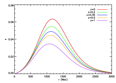
where $\Sigma^{2}=\Sigma_{ij}\Sigma^{ij}$ is the square of the background shear, and $\Theta$ the expansion parameter of a congruence of comoving geodesics (see (, García-Bellido & Haugbølle2009) for further details). For voids of practical interests this shear parameter is usually small (in particular for the simulated model $\epsilon\lesssim 0.06$, see fig. 1). Hence one would think that background shear effects can be neglected, in which case the equations for the density perturbations reduce, at a fixed radius $r$, to those of an FRW universe with the corresponding effective cosmological parameters at that $r$. We write this solution as

$$\delta_{0}(t,r)\propto\,D(\Omega(r),A(t,r)/A_{0}(r)),$$ (4)

where

$$D(\Omega,a) \equiv\frac{5}{2}\Omega\,h^{2}\,H(\Omega,a)\int_{0}^{a}\frac{da^{\prime}}{[a^{\prime}\,H(\Omega,a^{\prime})]^{3}}$$

$$=a\cdot{}_{2}F_{1}\left[1,2;\frac{7}{2};\frac{\Omega-1}{\Omega}\,a\right]$$ (5)

is the growth factor in an Open CDM universe with matter parameter $\Omega$, with ${}_{2}F_{1}(a,b;c;z)$ the Gauss hypergeometric function. The full density perturbation equation has the form (, Padmanabhan1996, Clarkson et. al,2009)

$$\ddot{\delta}+2H_{T}\dot{\delta}+(4\dot{H}_{T}+6H_{T}^{2})\delta={\cal O}\left(\Sigma^{2},\,\delta^{2}\right)\,.$$ (6)

In the small shear limit, $\Sigma\to 0$, we propose the following Ansatz as an approximate solution

$$\delta_{\alpha}(t,r)=\delta_{0}(t,r)\,\Big{(}1+\alpha\,\epsilon(t,\,r)\Big{)},$$ (7)

where the parameter $\alpha$ could, in principle, depend on $(t,\,r)$ and possibly also on the cosmological parameters.

II.3 The mass function in LTB models

Most of the information about the non-linear accretion of dark matter halos is encoded in the mass function $n(M)\,dM$: the comoving number density of halos with mass $M\in(M,M+dM)$. The first theoretical description of the mass function was developed by Press and Schechter (, Press & Schechter1974) (PS hereon) and later re-derived and extended by Bond et al. in the so-called excursion set formalism (, Bond et al.1991). Within this framework the abundance of halos can be predicted as the abundance of points in space in which the linear density contrast $\delta$ smoothed over a scale corresponding to the mass $M$ has crossed the spherical collapse threshold $\delta_{c}=1.686$. Although the PS prediction describes qualitatively well the mass function, it fails to reproduce its details (overpredicting the density of low mass objects and underpredicting massive ones). Nevertheless it is a remarkable achievement that one can estimate the abundance of non-linear structures using only linear perturbation theory and the assumption that $\delta$ is gaussian-distributed. The PS formula has been perfected using ellipsoidal collapse and empirical parametrizations (, Sheth & Tormen1999, Tinker et. al2008), so that $n(M)$ can be calculated to very good accuracy, often using one of the main results from this formalism: the mass function should be a universal (cosmology-independent) function of the variance of the linear density contrast field $\sigma(M,z)$ (, Jenkins et al.2000). Here we will use

$$n(M,z)=\frac{\rho_{M}}{M}g(\sigma)\left|\frac{d\,\ln\,\sigma}{dM}\right|,$$ (8)

where $\sigma\equiv\sigma(M,z)$ and $g(\sigma)$ is given by (Peacock, 2007):

$$g(\sigma)\equiv\frac{a\,b\,\nu^{b}+2\,c\,\nu^{2}(1+a\,\nu^{b})}{(1+a\,\nu^{b})^{2}}\exp(-c\,\nu^{2}),$$

$$(a,b,c)=(1.529,0.704,0.412),\,\,\,\nu\equiv\delta_{c}/\sigma.$$

We have also tried other parametrizations of the mass function (, Sheth & Tormen1999, Tinker et. al2008) and checked that our results did not depend significantly on this choice.

We follow the same rationale in order to calculate the mass function of halos at a given $r$ and $t$ in an LTB model: since the simulated void arises from a purely growing mode (i.e.: the Big Bang time is homogeneous), and perturbations grow in a self-similar fashion, it is reasonable to assume that, in order to calculate the variance of $\delta_{M}$ at $(t,r)$, we should rescale the variance $\sigma_{\rm out}(M,z)$ of the density perturbations outside the void, by a factor

$$f(t,r)=\frac{\delta_{\alpha}(t,r)}{\delta_{\alpha}(t,r\rightarrow\infty)}\,,$$ (9)

where the density contrast is computed theoretically according to Eq. (7), and evaluated in Fig. 2, with and without the shear correction. Thus, our model for the mass function $n(M,z,r)$ at a given radius $r$ is Eq. (8) with $\sigma(M,z)$ substituted by $\sigma_{\rm out}(M,z)\,f(t,r)$.

Note however, that our main results will be quoted in terms of the cumulative mass function within a sphere of radius $r$ centered at the origin of the LTB patch:

$$n(>M,<r,z)\equiv\frac{3}{4\pi\,r^{3}}\int_{0}^{r}r^{\prime 2}dr^{\prime}\int_{M}^{\infty}dM^{\prime}\,n(M^{\prime},r^{\prime},z),$$ (10)

since this observable has better statistics.

III The simulation and the halo catalog

A more detailed description of the simulation we have used can be found in (Alonso et al., 2010) (simulation $\mathcal{H}$). It has $960^{3}$ particles in a box of size $L=2400$ Mpc $h^{-1}$, which sets the mass resolution to $m_{p}=4.2\times 10^{12}\,M_{\odot}\,h^{-1}$. The simulated void has a size of $r_{0}=1100$ Mpc, a transition width of $\Delta r/r_{0}=0.3$ and an underdensity of $\Omega_{\rm in}=0.25$ (see section II.1). The background cosmology is Einstein-de Sitter ($\Omega=1$) with $h_{\rm out}=0.43$. The small-scale perturbations are set using a power spectrum with $n_{s}=1$ and $\sigma_{8}=0.9$. It must be noted that an LTB void with these parameters is in fact ruled out, since the supernovae and baryon acoustic oscillation data seems to be mutually in conflict given a particular LTB profile (, Zumalacarregui et. al,2012). We only use this simulation with a large background shear as a toy model to test our Ansatz about the mass function. The technique used to simulate LTB voids is based on setting the initial conditions (IC) appropriately by modifying the IC generator to take into account the large-scale perturbation induced by the presence of the void. This must be done at a high enough redshift so that the void can be regarded as a linear perturbation. A modified version of the 2LPT code (, Crocce et. al,2006) was used for this stage. Once the ICs are set, they are plugged into Gadget2 (, Springel2005), which we run in pure tree-mode.

The halo catalog has been extracted using the AMIGA halo finder AHF (, Knollmann & Knebe2009, Gill et al.2004). It maps the particle content to an adaptively smoothed density field and locates the position of possible halos as local overdensities. Once the gravitationally bound particles around these have been extracted, the extent and mass of each halo is computed as:

$$M(r_{\rm vir})=\frac{4\pi}{3}r_{\rm vir}^{3}\rho_{c}\,\Delta,$$ (11)

where we have used $\Delta=200$ as a collapse threshold (e.g. , Knebe et al.2011).

IV Results

Figure 2: Cumulative mass function for halos inside spheres of different radii compared with the theoretical prediction without the background shear correction ($\alpha=0$, top panel) and with a first order shear correction, where $\alpha=2\,\forall\,r,\,t$ (bottom panel).

$r$ (Mpc)	$\xi_{N}^{2}(\alpha=0)$	$\xi_{N}^{2}(\alpha=2)$
300	0.093	0.112
600	0.682	0.104
900	8.321	0.173
1200	2.394	0.047
1500	1.474	0.072
1800	0.478	0.050
2100	0.177	0.032
2400	0.095	0.061

Table 1: Goodness of fit of our theoretical approach with and without a first order shear correction for different radii at $z=0$. Similar results hold at all other redshifts (see table 2).

$z$	$\xi_{N}^{2}(\alpha=0)$	$\xi_{N}^{2}(\alpha=2)$
0	1.620	0.072
0.2	1.163	0.065
0.35	1.411	0.042
0.5	0.667	0.047
1	3.494	0.824

Table 2: Goodness of fit of our theoretical approach with and without a 1-st order shear correction for different redshifts (summing over all radii).

Figure 3: Top panel: dependence of $\xi_{N}^{2}$ (eq. 12) with the value of the shear correction term $\alpha$ at different $r$ and $t$. Bottom panel: best fit value of $\alpha$ for different radii and redshifts, showing a mild evolution with $r$.

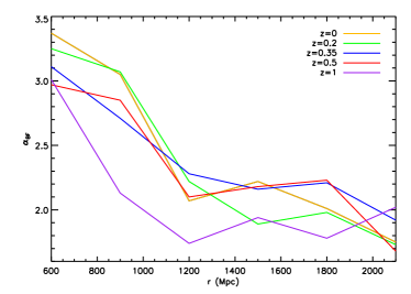
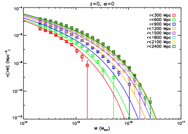
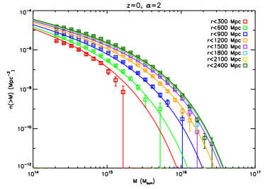
Once the halos have been identified, we can compute $n(>M,<r,z)$ merely by counting the number of halos with mass above $M$ inside a sphere of radius $r$ and dividing by the comoving volume of this sphere. The results are shown in figure 2. It is easy to see (top panel) that, while approximating the growth of perturbations by its 0-th order in $\epsilon$ (eq. 4) yields a reasonably good fit at small and large radii (where the background shear vanishes), it fails to reproduce the halo abundances at intermediate radii. In the bottom panel we can see, however, that adding a non-zero 1-st order correction (eq. 7) solves this problem. Furthermore, we have found that this correction seems to be almost independent of $r$ and $t$, with $\alpha\sim 2$.

We have quantified the goodness of fit of our approach (with and without the shear correction term) using the measure:

$$\xi_{N}^{2}(r,z)\equiv\frac{1}{N-1}\sum_{i}^{N}\left(\frac{n(>M_{i},<r,z)-n_{i}(r)}{n(>M_{i},<r,z)}\right)^{2}.$$ (12)

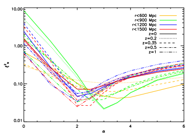
Here $n(>M,<r,z)$ is given in section II.3, $n_{i}(r)$ is the cumulative mass function obtained from the simulation for a mass $M_{i}$ within a sphere of radius $r$, and $N$ is the number of mass bins. Figure 3 (top panel) shows the value of $\xi_{N}^{2}$ for different choices of $\alpha$ at different $r$ and $z$. A value of $\alpha\sim 2$, found as the median of the best-fit values for all the calculated curves, gives a good fit in all cases with only a very mild dependence on $r$ and $t$ (shown on the bottom panel of Fig. 3). The improvement due to the shear-correction term can also be seen in table 1, in which we have calculated the goodness of fit with and without the shear correction for different radii at $z=0$. Table 2 shows the same result for different redshifts summing over all radii. This improvement is especially evident at intermediate radii, where $\epsilon$ is larger and therefore its effects more important.

It would be extremely interesting to investigate whether and how the value of $\alpha$ depends on the cosmological parameters: if this parameter turned out to be independent of the void model, one should be able to predict its value from some approximation in perturbation theory. However, this is work in progress and we defer the presentation of it to future work that will also make use of better resolved simulations.

V Discussion & conclusions

We have extracted the halo content from an LTB N-body simulation and analyzed the halo abundances at different masses and radii. The main conclusions from this study are:

• The theoretical description of the halo mass function in FRW cosmologies can be fully extended to LTB void models by adding just one parameter ($\alpha$) that accounts for the effect of the background shear on the evolution of matter density perturbations.

• The value of this parameter ($\sim 2$) seems to be constant in time and only mildly dependent on the position in the void. Whether this value depends weakly on the void model is still work in progress.

If the shear correction turns out to be practically independent of the void model parameters, halo abundances could potentially be used to constrain the amount of background shear, a crucial test for general inhomogeneous cosmological models. A toy model that has been considered in the past in connection with LTB scenarios, and which could benefit from our analysis of background shear, is the swiss-cheese model (, Marra et. al,2007, Biswas & Notari,2008, Marra et. al,2008). We leave for the future such investigation. It is also worthwhile exploring whether our results apply to voids of astrophysical scales, of tens of Mpc, since they could have an effect on the modelling of the environmental dependence of dark matter halo properties, as well as the backreaction of non-linear gravitational collapse on the background evolution.

References

- (1) Alnes H., Amarzguioui M., Gron O. 2006, PRD, 73, 083519
- Alonso et al. (2010) Alonso D., García-Bellido J., Haugbølle T., Vicente J. 2010, PRD, 82, 123530
- (3) Biswas T., Notari A. 2008, JCAP, 0806, 021
- (4) Biswas T., Notari A., Valkenburg W. 2010, JCAP, 1011, 030
- (5) Bond J. R., Cole S., Efstathiou G., Kaiser N. 1991, ApJ, 379, 440
- (6) Celerier M. 2000, A&A, 353, 63
- (7) Clarkson C., Clifton T., February S. 2009, JCAP, 0906, 025
- (8) Crocce M., Pueblas S., Scoccimarro R. 2006, MNRAS, 373, 369
- (9) Enqvist K., Mattsson T. 2007, JCAP, 0702, 019
- (10) García-Bellido J., Haugbølle T. 2008a, JCAP, 0804, 003
- (11) García-Bellido J., Haugbølle T. 2008b, JCAP, 0809, 016
- (12) García-Bellido J., Haugbølle T. 2009, JCAP, 0909, 028
- (13) Gill, S. P. D. and Knebe, A. and Gibson, B. K., 2004, MNRAS, 351, 399
- (14) Goldberg D. M., Vogeley M. S. 2004, ApJ, 605, 1
- (15) Jenkins et al. 2000, MNRAS, 321, 372
- (16) Knebe, A. et al., 2011, MNRAS, 451, 2293
- (17) Knollmann S. R., Knebe A., 2009, ApJS, 182, 608
- (18) Lavallaz A., Fairbairn M. 2011, PRD, 84, 083005
- (19) Marra V., Kolb E. W., Matarrese S. 2007, PRD, 76, 123004
- (20) Marra V., Kolb E. W., Matarrese S., Riotto A. 2008, PRD, 77, 023003
- (21) Marra V., Pääkönen M., Valkenburg W. 2012, arXiv:1203.2180
- (22) Martino M. C., Sheth R. K. 2009, MNRAS, 394, 2109
- (23) Moss A., Zibin J. P., Scott D. 2011, PRD, 83, 103515
- (24) Nishikawa R., Chul-Moon Yoo, Ken-ichi N. 2012, arXiv:1202.1582v1 [astro-ph.CO]
- (25) Padmanabhan, T., “Cosmology and Astrophysics through Problems”, Cambridge University Press, (1996).
- Peacock (2007) Peacock J. A. 2007, MNRAS, 379, 1067
- (27) Press W. H., Schechter P. 1974, ApJ, 187, 425
- (28) Sheth R. K., Tormen G. 1999, MNRAS, 308, 119
- (29) Sinclair B., Davis T. M., Haugbølle T. 2010, ApJ, 718, 1445
- (30) Springel V. 2005, MNRAS, 364, 1105
- (31) Tinker J. L., Kravtsov A. V., Klypin A., Abazajian K., Warren M. S., Yepes G., Gottlober S., Holz D. E. 2008, ApJ, 688, 709
- (32) Tomita K. 2001, MNRAS, 326, 287
- (33) Zehavi I., Riess A. G., Krishner R. P., Dekel A. 1998, ApJ, 503, 483
- (34) Zhang P., Stebbins A. 2011, PRL, 107, 041301
- (35) Zibin J. P. 2008, PRD, 78, 043504
- (36) Zibin J. P., Moss A. 2011, Class. Quant. Grav., 28, 164005
- (37) Zumalacarregui M., García-Bellido J., Ruiz-Lapuente P. 2012, arXiv:1201.2790 [astro-ph.CO]