Combining Neutrino Oscillation Experiments with the Feldman-Cousins Method

Abstract

In this article we describe how two or more experimental results can be combined within the procedure of Feldman and Cousins, to provide combined confidence limits on the physical parameters of interest. We demonstrate the technique by combining the recent electron neutrino appearance results from T2K and MINOS. Our best fit point is $\sin^{2}2\theta_{13}=0.08\,(0.11)$ and $\delta=1.1\,(2.0)\pi$; in addition we exclude $\sin^{2}2\theta_{13}=0$ at $2.7\sigma$ ($2.8\sigma$) for the normal (inverted) neutrino mass hierarchy.

1 Introduction

In order to obtain global constraints on physical parameters, it is often necessary to combine the results of two or more experiments with sensitivities to the same parameters. Such combinations can be performed with different levels of sophistication, depending on what information is available about the original measurements. In the absence of detailed information, relatively crude combinations, e.g. by simply summing log-likelihood values, can be useful, but these results will always be subject to caveats.

In this work, we describe a method to combine results which requires somewhat detailed experimental information, but which focuses on obtaining correct coverage of the parameter space under study, by producing a combined likelihood curve from the joint data set of the experiments, and using the Feldman-Cousins method [1] to define acceptance regions for each point in the parameter space. We will describe the inputs that would be required from an experiment to enable its inclusion in such an analysis in § 2.1. We also present, as an example of the technique, the combination of the recent electron neutrino appearance results from the long baseline experiments MINOS and T2K. This example is particularly pertinent, since the parameter $\theta_{13}$ is known to be near a physical bound; the Feldman-Cousins technique was developed to deal with such cases, since conventional methods for determining acceptance regions can produce incorrect coverage or null contours. A comparison will also be made between our method and one where fixed log-likelihood differences are used to produce the contours.

1.1 The example: Constraints on $\theta_{13}$ from MINOS and T2K

Neutrino oscillations, a now well established phenomenon [6, 7, 8, 9, 10, 11], can be parametrised by the PMNS mixing matrix [12, 13], assuming a minimal 3-flavour mixing model. All of the mixing angles in this matrix have now been measured to be non-zero, including the angle $\theta_{13}$ [4, 5], which governs muon to electron neutrino oscillations in the atmospheric ($L/E$) regime. The $\mathcal{C\!P}$-violation parameter $\delta$ is as yet unknown. In the appearance channel T2K has found an excess of electron neutrino events in a muon neutrino beam, suggesting that $\theta_{13}$ is non-zero, with a significance of $2.5\sigma$ [2]. MINOS has also found an excess of events, excluding $\theta_{13}=0$ at 89% CL [3]. We will combine the results of these two experiments to get improved constraints on $\theta_{13}$ from electron neutrino appearance measurements, as well as the $\mathcal{C\!P}$-violation parameter $\delta$. In the disappearance channel, $\theta_{13}$ has recently been measured to be non-zero by two different reactor experiments, Daya Bay [4] and RENO [5].

MINOS and T2K are both long baseline accelerator neutrino oscillation experiments, in which a predominantly $\nu_{\mu}$ beam is created by colliding protons onto a target, then magnetically focusing the resultant charged mesons and allowing them to decay. The neutrino beam thus produced is sampled at source by a near detector, and several hundred kilometers away by a far detector. Details of the individual experiments’ setups are described elsewhere [14, 15]. Both experiments are at an atmospheric $L/E$, but their different energies and baselines (MINOS is at 735 km and has a beam peaked at 3 GeV whereas T2K is at 295 km with a beam peak of 0.6 GeV), along with different detector technologies and analysis techniques lead to different systematic errors, as well as different sensitivities to the oscillation parameters. Both experiments use the difference in the numbers of electron-neutrino-like events observed in their far detectors from those predicted to constrain $\theta_{13}$. Both analyses are performed with the Feldman-Cousins method.

2 Method to Combine Fits

In order to combine the data from two or more experiments, the binned data from all experiments are considered together, as a single larger experiment. The Feldman-Cousins technique is then used to produce confidence contours based on the combined data.

2.1 Inputs to the analysis

In order to perform our analysis, the data from each experiment are required, along with Monte Carlo expectation values. Specifically, these consist of:

1. The number of data events in each analysis bin for each experiment.

2. The expected number of events in each analysis bin, as a function of the parameters $\bm{\theta}$ to be fitted over, in our example $(\sin^{2}2\theta_{13},\delta)$. The number of events will vary smoothly with the oscillation parameters, so a set of values on a grid, which can be numerically interpolated for intermediate points, is suitable for this purpose.

3. The correlated bin-by-bin systematic errors for each experiment, encoded in covariance matrices, as a function of the parameters $\bm{\theta}$. We therefore require that the calculation of a covariance matrix from the underlying sources of systematic uncertainty (cross-section errors, beam-line uncertainties etc.) has been performed by each experiment. We assume that both experimental and theoretical uncertainties are included in the matrix.

Note that although we assume that the bin-to-bin correlations within each experiment will be provided, in general there will also be correlations between experiments, which may be important for the final result. This detail is discussed in § 2.6. It should be noted further that in order to be combined consistently, we require that the original analyses make essentially the same physics assumptions; for example the values of mixing parameters other than those in the fit.

2.2 The Feldman-Cousins technique

The Feldman-Cousins technique is a method for generating acceptance regions within the classical framework for interval calculation [17]. Its distinctive feature is that when choosing which data values $\bm{n}$ to include in the acceptance for a given $\bm{\theta}$, the candidates are ranked by the relative likelihood of observing $\bm{n}$ at $\bm{\theta}$, with respect to the likelihood of observing $\bm{n}$ at the best fit point for that data. The use of relative rather than absolute likelihoods means that data values which are unlikely for all points in the parameter space will still be included in the acceptance region for some $\bm{\theta}$, avoiding the problem of null contours for some data values. The method also automatically produces a smooth transition between one- and two-sided intervals depending on the observed data, with correct coverage throughout.

The key procedural step in the technique is the generation of a large number of “toy” Monte Carlo experiments at many positions in the parameter space, in order to identify the relative likelihood limit for each point which will give the correct coverage. For our example, $10^{4}$ toy experiments were generated at each value of $\bm{\theta}$ considered. For each toy experiment result $\bm{n}$, a fit is performed for $\bm{\theta}_{\mathrm{best}}$ using a likelihood function $\ln\mathcal{L}$. The difference, $\Delta(\ln\mathcal{L})$, in the log likelihood between the best fit point $\bm{\theta}_{\mathrm{best}}$, and the value $\bm{\theta}$ actually used to generate the toy experiment, is calculated.

Using the $\Delta(\ln\mathcal{L})$ from all toy experiments, a value $\Delta(\ln\mathcal{L})_{\mathrm{crit}}$ is calculated, such that some fixed proportion, say 90%, of toy experiments satisfy the condition

$$\Delta(\ln\mathcal{L})\leq\Delta(\ln\mathcal{L})_{\mathrm{crit}}.$$ (1)

The condition (1) defines an acceptance region with 90% probability for the value of $\bm{\theta}$ in question. Repeating the procedure for all values of $\bm{\theta}$, a surface $\Delta(\ln\mathcal{L})_{\mathrm{crit}}(\bm{\theta})$ is calculated.

A fit is then made to the real data using our likelihood function, obtaining a best fit point $\bm{\theta}_{\mathrm{best}}$, and a corresponding log-likelihood value $(\ln\mathcal{L})_{\mathrm{best}}$. A log-likelihood surface $(\ln\mathcal{L})(\bm{\theta})$ is also calculated on a grid in $\bm{\theta}$. We then draw our confidence interval, using the condition (1), with $\Delta(\ln\mathcal{L})=(\ln\mathcal{L})(\bm{\theta})-(\ln\mathcal{L})_{\mathrm{best}}$, at each point in $\bm{\theta}$-space to decide whether the point should be included in the contour.

2.3 Toy experiment generation

The toy Monte Carlo (MC) is required to give a number of events for each analysis bin, $n_{i}^{\mathrm{obs}}$, based on the expected number of events $n_{i}^{\mathrm{exp}}$ for a given value of $\bm{\theta}$, allowing for fluctuations due to systematic  and statistical uncertainties. The expected number of events used is the total (i.e. signal plus background) expectation, so that both signal and background counts fluctuate between our toy experiments. The main complication in the MC is to ensure that correlations between the bin values are taken into account.

Expressing the systematic uncertainties as absolute shifts (“tweaks”) $x_{i}$ in the expected number of events in each bin, we can write

$$n_{i}^{\mathrm{exp}}\to n_{i}^{\mathrm{exp}}+x_{i}.$$ (2)

Our method makes the common assumption that the systematic errors follow a multivariate normal distribution; that is, their joint pdf $f_{\mathrm{syst}}(\bm{x})$ follows

$$f_{\mathrm{syst}}(\bm{x})\propto e^{-\frac{1}{2}\bm{x}^{\top}V^{-1}\bm{x}},$$ (3)

where $V$ is the covariance matrix for the $x_{i}$.

Since $V$ is a symmetric, positive-definite matrix, we can use the method of Cholesky decomposition [16] to find an upper-diagonal matrix $L$ such that

$$V=L^{\top}L.$$ (4)

We can then use the matrix $L^{\top}$ as a transformation to enable us to generate the vector $\bm{x}$ from another vector of random variables $\bm{y}$, such that

$$\bm{x}=L^{\top}\bm{y}.$$ (5)

One can show by trivial matrix algebra that we can rewrite the factor in the exponential in (3) as

$$\bm{x}^{\top}V^{-1}\bm{x}=\bm{y}^{\top}\bm{y},$$ (6)

and so we deduce that if we generate the $y_{i}$ independently on a normal distribution with unit standard deviation, then the vector $\bm{x}$ generated using (5) will have the desired covariance properties. From now on, unless otherwise stated, we assume that $n_{i}^{\mathrm{exp}}$ has been modified for systematics using this prescription, so that it is now a function $n_{i}^{\mathrm{exp}}(\bm{\theta},\bm{y})$ of both $\bm{\theta}$ and $\bm{y}$. We will also use $f_{\mathrm{syst}}(\bm{y})$ to refer to the probability density function (pdf) of the random vector $\bm{y}$.

Having taken account of systematics, a number of events for each bin can be generated using Poisson statistics, i.e. on a pdf

$$g_{\mathrm{pois}}(n_{i}^{\mathrm{obs}};n_{i}^{\mathrm{exp}}(\bm{\theta},\bm{y}))=\frac{(n_{i}^{\mathrm{exp}}(\bm{\theta},\bm{y}))^{n_{i}^{\mathrm{obs}}}}{n_{i}^{\mathrm{obs}}!}e^{-n_{i}^{\mathrm{exp}}(\bm{\theta},\bm{y})},$$ (7)

where the $y_{i}$ must be generated separately for each toy experiment.

2.4 The likelihood function $\ln\mathcal{L}$

When performing our fits, the value of the systematic “tweak” parameters is allowed to vary, so our likelihood function must include penalty terms to account for the finite uncertainty in these parameters. We define a likelihood function including both systematic and statistical terms, as a function of $\bm{\theta}$ and $\bm{y}$, using the same pdfs we used to generate the toy experiments:

$$\mathcal{L}(\bm{n}^{\mathrm{obs}};\bm{y},\bm{\theta}) =\prod_{i=0}^{N}\left(g_{\mathrm{pois}}(n_{i}^{\mathrm{obs}};n_{i}^{\mathrm{exp}}(\bm{\theta},\bm{y}))\right)f_{\mathrm{syst}}(\bm{y})$$ (8)

$$\propto\prod_{i=0}^{N}\left((n_{i}^{\mathrm{exp}}(\bm{\theta},\bm{y}))^{n_{i}^{\mathrm{obs}}}e^{-n_{i}^{\mathrm{exp}}(\bm{\theta},\bm{y})}\right)e^{-\frac{1}{2}\bm{y}^{\top}\bm{y}},$$

where we have dropped factors independent of $(\bm{\theta},\bm{y})$. As is standard, minimisation is actually performed on the logarithm of the likelihood function since this is a simpler process, and is equivalent as $\ln\mathcal{L}$ is a monotonic function of $\mathcal{L}$. This function is given by

$$-2\ln\mathcal{L}=\sum_{i=0}^{N}\left(2n_{i}^{\mathrm{exp}}(\bm{\theta},\bm{y})-2n_{i}^{\mathrm{obs}}\ln(n_{i}^{\mathrm{exp}}(\bm{\theta},\bm{y}))+y_{i}^{2}\right).$$ (9)

In the case that we do not wish to fit for systematics (e.g. for direct comparison with other analyses), we use the simpler function

$$-2\ln\mathcal{L}=2\sum_{i=0}^{N}\left(n_{i}^{\mathrm{exp}}-n_{i}^{\mathrm{obs}}\ln n_{i}^{\mathrm{exp}}\right),$$ (10)

where the $n_{i}^{\mathrm{exp}}$ are no longer functions of $\bm{y}$.

2.5 Performing the fit

We perform the minimisation of $(-2\ln\mathcal{L})$ using the MINUIT minimiser via the interface provided by the ROOT framework [18]. The derivatives $\frac{\partial\ln\mathcal{L}}{\partial y_{i}}$ are calculated analytically to improve performance. The fit requires as inputs the vector $\bm{n}^{\mathrm{exp}}$, and the Cholesky decomposition $L$ of its covariance matrix $V$, at every point in $\bm{\theta}$ space. These inputs are generated on a grid in $\bm{\theta}$ in advance and then picked out by interpolation.

The fit is split into two nested components: a “top-level fit” over the parameters $\bm{\theta}$, and another fit performed over $\bm{y}$ which is called by the top-level fit to find the best $(\ln\mathcal{L})$ value for a given $\bm{\theta}$. $\sin^{2}(2\theta_{13})$ is constrained to lie in the physical region [0,1]. The $\bm{y}$ are allowed to float freely, but all $n_{i}^{\mathrm{exp}}$ are constrained to remain above zero (actually $10^{-5}$) regardless of the $\bm{y}$.

2.6 Correlated systematic errors

When combining experiments with some common systematic error sources, it is necessary to calculate the correlation coefficients between the bins of the two experiments. In order to do this we must identify the common systematic uncertainties, and get from each experiment the contributions of these error sources to the total errors on each bin.

Once this information is available, the cross-terms in the covariance matrix can be calculated. Assuming Gaussian errors, we express the number of events in each bin $i$ as

$$n_{i}=\overline{n_{i}}+\sigma^{\mathrm{uncorr}}_{i}y_{i}+\sum_{\alpha}c_{i\alpha}z_{\alpha},$$ (11)

where the $y_{i}$ and $z_{\alpha}$ are independent normally distributed random variables with ($\sigma=1$, $\mu=0$), $\alpha$ indexes the correlated error sources and the $c_{i\alpha}$ give the contribution of the error source $\alpha$ to the error on bin $i$. $\sigma^{\mathrm{uncorr}}_{i}$ is the uncorrelated component of the systematic error on bin $i$. From (11), it is easy to show that

$$V_{ij}\equiv\langle(n_{i}-\overline{n_{i}})(n_{j}-\overline{n_{j}})\rangle=\sum_{\alpha}c_{i\alpha}c_{j\alpha}+\delta_{ij}(\sigma^{\mathrm{uncorr}}_{i})^{2}.$$ (12)

3 Our Combination Example

In our example we combine the electron neutrino appearance results of two long baseline experiments: MINOS [3] and T2K [2]. The inputs we take from each experiment are the expected number of electron neutrino events (as a function of $\theta_{13},\delta$), in each bin, along with the covariance matrices of the systematic errors between the bins in each experiment. The T2K result consists of a single bin, and the MINOS result of fifteen bins (five of energy times three of the Library Event Matching particle identification parameter).

3.1 Validation

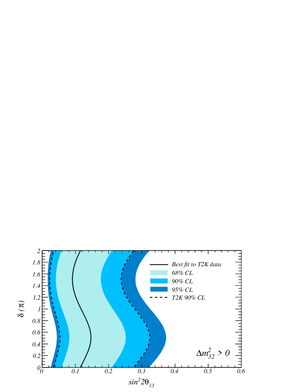
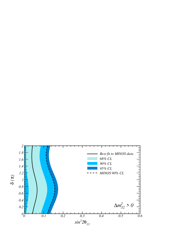
To validate our method, we have reproduced the results of both the T2K and MINOS analyses individually. There are some slight differences in the ways in which the two experiments perform their analyses, which must be considered when validating our method, and when making a combination of their results. One difference is that MINOS minimise over the systematic errors in their likelihood function, whereas T2K do not. Since in general it may be advantageous to minimise over the systematic errors, we do minimise over systematics in our example fit. Another difference is that T2K show their results for $\sin^{2}2\theta_{13}$ at a fixed value of $2\sin^{2}\theta_{23}=1$, whereas MINOS show the combination $2\sin^{2}\theta_{23}\sin^{2}2\theta_{13}$, by throwing $\theta_{23}$ between its errors and then choosing $\theta_{13}$ to keep this quantity fixed in each toy experiment. The systematic errors that MINOS have provided us with, however, do not include any uncertainty in the oscillation parameters (a fixed value of $2\sin^{2}\theta_{23}=1$ is used). This means that our combination can be interpreted as constraining $\sin^{2}2\theta_{13}$ at $2\sin^{2}\theta_{23}=1$. The other oscillation parameters used for calculation of the input distributions were: $\sin^{2}2\theta_{12}=0.87$, $\Delta m^{2}_{21}=7.6\times 10^{-5}\,\textrm{eV}^{2}$ and $\Delta m^{2}_{32}=2.3\times 10^{-3}\,\textrm{eV}^{2}$. For T2K, the provided inputs actually used $\Delta m^{2}_{32}=2.4\times 10^{-3}\,\textrm{eV}^{2}$, but changing to $\Delta m^{2}_{32}=2.3\times 10^{-3}\,\textrm{eV}^{2}$ made negligible difference to the result.

The validation results are shown in Figures 1 and 2, for T2K and MINOS respectively. In both cases, we find good agreement with the published contours.

Figure 1: Reproduction of the T2K results: we find good agreement with the published contours [2]. In addition, we exclude $\sin^{2}2\theta_{13}=0$ at $2.5\sigma$.

Figure 2: Reproduction of the MINOS results: we find good agreement with the published contours [3].

3.2 Possibly Correlated Systematic Errors

In order to combine the errors from both experiments into a single covariance matrix, we need to consider the systematic errors that may be correlated between them. In the case of our example, most of the sources of error cited in [3, 2] can be assumed to be uncorrelated between experiments, due to the different experimental set-ups and different neutrino energies involved. However, cross section uncertainties between the single T2K bin (energies up to 1.25 GeV) and the MINOS low energy (1-2 GeV) bins are potentially correlated.

To assess the necessity of evaluating this correlation, we performed a worst-case estimate of its effect, by assuming complete correlation between the T2K cross-section error, and the total MINOS cross-section plus flux error [19]. These numbers were chosen as they will overestimate the effect and are available from the cited publications. Running our analysis with and without these worst-case correlations included, we found negligible difference in the results. We therefore conclude that we can neglect correlated errors for the MINOS-T2K combination at this point, though this may not be true for later data sets, if cross-section errors assume a greater relative importance.

It should be noted for the future that whilst one reactor experiment could be combined with MINOS and T2K without needing to account for correlations (very different energies, flux, baseline etc.), if multiple reactor experiments were to be included some effort would be needed to calculate the correlations between their errors. The same would be true if another long-baseline neutrino experiment with similar peak neutrino energy as either MINOS or T2K were to be included.

3.3 Results

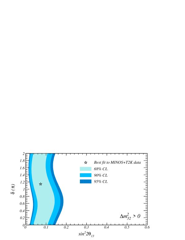
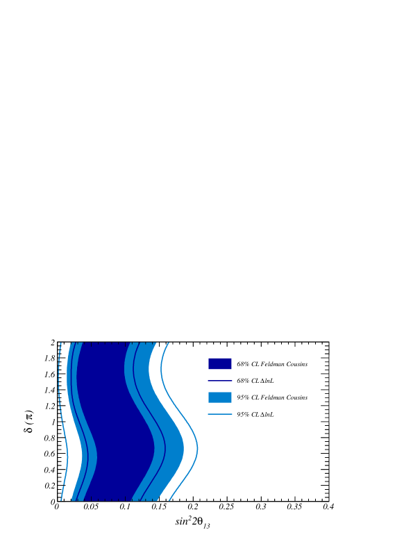
As previously mentioned, we take the profile likelihood, minimising over systematic errors, in our final fit. We also minimise over $\delta$ when calculating the minimum value of our likelihood function, since the combination of the two experiments gives slight sensitivity to $\mathcal{C\!P}$-violation. The normal and inverted neutrino mass hierarchies are treated separately. We find allowed regions of: $0.02\,(0.03)<\sin^{2}2\theta_{13}<0.16\,(0.21)$ at 95% C.L., $0.03\,(0.04)<\sin^{2}2\theta_{13}<0.15\,(0.19)$ at 90% C.L., and $0.04\,(0.05)<\sin^{2}2\theta_{13}<0.12\,(0.16)$ at 68% C.L., for the normal (inverted) neutrino mass hierarchy, where we have taken the profile likelihood, minimising over $\delta$, for each value of $\sin^{2}2\theta_{13}$, both for the data and during the calculation of the critical values of $\Delta(2\textrm{ln}\mathcal{L})$ ($\delta$ was thrown uniformly across $[0,2\pi)$ in the generation of the toy experiments), to give one-dimensional confidence intervals. Two-dimensional confidence intervals are shown in Figure 3. No values of $\delta$ can be ruled out at $1\sigma$. The significance of the neutrino mass hierarchy preference, calculated by generating toy experiments about the global best fit point (which happens to be in the inverted neutrino mass hierarchy), and seeing what fraction of toy experiments had their global best fit point in the inverted mass hierarchy, is negligible. The best fit values of the oscillation parameters are $\sin^{2}2\theta_{13}=0.08\,(0.11)$ and $\delta=1.1\,(2.0)\pi$ for the normal (inverted) neutrino mass hierarchy. Our best fit value is compatible with the results presented in [20]. We exclude $\sin^{2}2\theta_{13}=0$ at $2.7\sigma$ ($2.8\sigma$) for the normal (inverted) neutrino mass hierarchy.

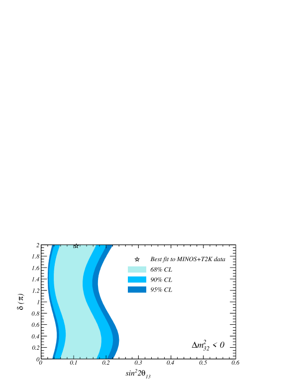
For comparison, in Figure 4 we show the contours that would be obtained by selecting an allowed region using a fixed value of $\Delta(2\textrm{ln}\mathcal{L})$. The regions obtained using the Feldman-Cousins approach are significantly narrower than those from the fixed log-likelihood contours.

Figure 3: The Feldman Cousins 68%, 90% and 95% confidence level contours for the combined electron neutrino appearance measurement of T2K and MINOS, for normal (top) and inverted neutrino mass hierarchies. We exclude $\sin^{2}2\theta_{13}=0$ at $2.7\sigma$, in the normal hierarchy.

Figure 4: The Feldman-Cousins confidence intervals and those obtained by placing the contour at a fixed $\Delta(2\textrm{ln}\mathcal{L})$ elevation. Shown here are the 95% CL allowed region (and corresponding $\Delta(2\textrm{ln}\mathcal{L})=5.99$ contour) and 68% CL allowed region (and corresponding $\Delta(2\textrm{ln}\mathcal{L})=2.30$ contour). The Feldman-Cousins allowed regions are significantly narrower than those formed using fixed $\Delta(2\textrm{ln}\mathcal{L})$ elevations.

4 Conclusions

We have demonstrated the combination of multiple experimental results with the Feldman-Cousins method. Details of the inputs from experiments needed for inclusion in such fits are outlined in § 2.1.

We would like to thank the MINOS and T2K collaborations for their help with this work. In particular we would like to thank: Ruth Toner and Lisa Whitehead, from MINOS, and Josh Albert, from T2K, for answering our many questions and helping with the validation of this work. We are also indebted to Louis Lyons for useful discussions. We acknowledge the support of STFC, U.K.

References

- [1] G.J. Feldman and R.D. Cousins, “Unified approach to the classical statistical analysis of small signals”, Phys. Rev. D 57, 3873 (1998)
- [2] K. Abe et al. (T2K Collaboration), “Indication of Electron Neutrino Appearance from an Accelerator-produced Off-axis Muon Neutrino Beam”, Phys. Rev. Lett. 107, 041801 (2011)
- [3] P. Adamson et al. (MINOS Collaboration), “Improved search for muon-neutrino to electron-neutrino oscillations in MINOS”, Phys. Rev. Lett. 107, 181802 (2011)
- [4] F. P. An et al. (Daya Bay Collaboration), “Observation of Electron-Antineutrino Disappearance at Daya Bay”, arXiv:1203.1669v1 (2012)
- [5] J. K. Ahn et al. (RENO Collaboration), “Observation of Reactor Electron Antineutrino Disappearance in the RENO Experiment”, arXiv:1204.0626v2 (2012)
- [6] B. Aharmim et al. (SNO Collaboration), “Independent Measurement of the Total Active Solar Neutrino Flux Using an Array of Proportional Counters at the Sudbury Neutrino Observatory”, Phys.Rev. Lett. 101, 111301 (2008)
- [7] S. Abe et al. (KamLAND Collaboration), “Precision Measurement of Neutrino Oscillation Parameters with KamLAND”, Phys. Rev. Lett. 100, 221803 (2008)
- [8] Y. Ashie et al. (Super-Kamiokande Collaboration), “Measurement of atmospheric neutrino oscillation parameters by Super-Kamiokande I”, Phys. Rev. D 71, 112005 (2005)
- [9] K. Abe et al. (Super-Kamiokande Collaboration), “Measurement of Atmospheric Neutrino Flux Consistent with Tau Neutrino Appearance”, Phys. Rev. Lett. 97, 171801 (2006)
- [10] P. Adamson et al. (MINOS Collaboration), “Measurement of the neutrino mass splitting and flavor mixing by MINOS”, Phys.Rev.Lett. 106, 181801 (2011)
- [11] P. Adamson et al. (MINOS Collaboration), “First Direct Observation of Muon Antineutrino Disappearance”, Phys. Rev. Lett. 107, 021801 (2011)
- [12] B. Pontecorvo, “Inverse beta processes and nonconservation of lepton charge”, Sov. Phys. JETP 7, 172 (1958)
- [13] Z. Maki, M. Nakagawa and S. Sakata, “Remarks on the Unified Model of Elementary Particles”, Prog. Theor. Phys. 28, 870 (1962)
- [14] P. Adamson et al. (MINOS Collaboration), “The magnetized steel and scintillator calorimeters of the MINOS experiment”, Nucl. Inst. & Meth. A 596, 2, 190-228 (2008)
- [15] K. Abe et al. (T2K Collaboration), “The T2K Experiment”, Nucl. Inst. & Meth. A 659, 1, 106-135 (2011)
- [16] W.H. Press, S.A. Teukolsky, W.T. Vetterling and B.P. Flannery, “Numerical Recipes in C++ (Second Edition)”, 99-101 (2002)
- [17] J. Neyman, “Outline of a Theory of Statistical Estimation Based on the Classical Theory of Probability”, Phil. Trans. of the Royal Society of London. Series A, Math. and Phys. Sciences, Vol. 236, No. 767, 333-380 (1937)
- [18] R. Brun and F. Rademakers, “ROOT - An Object Oriented Data Analysis Framework”, Proc. AIHENP’96 Workshop, Lausanne, Sep. 1996, Nucl. Inst. & Meth. in Phys. Res. A 389, 81-86 (1997), see also http://root.cern.ch/
- [19] P. Adamson et al. (MINOS Collaboration), “New constraints on muon-neutrino to elecron-neutrino transitions in MINOS”, Phy.Rev.(Rapid Communications) D82:051102 (2010)
- [20] T. Schwetz, M. Tórtola and J. W. F. Valle, “Where we are on : Addendum to “Global Neutrino Data and Recent Reactor Fluxes: Status of Three-Flavour Oscillation Parameters” ”, arXiv:1108.1376v1 [hep-ph] (2011)