Towards Understanding the Fundamentals of Mobility in Cellular Networks
Abstract
Despite the central role of mobility in wireless networks, analytical study on its impact on network performance is notoriously difficult. This paper aims to address this gap by proposing a random waypoint (RWP) mobility model defined on the entire plane and applying it to analyze two key cellular network parameters: handover rate and sojourn time. We first analyze the stochastic properties of the proposed model and compare it to two other models: the classical RWP mobility model and a synthetic truncated Levy walk model which is constructed from real mobility trajectories. The comparison shows that the proposed RWP mobility model is more appropriate for the mobility simulation in emerging cellular networks, which have ever-smaller cells. Then we apply the proposed model to cellular networks under both deterministic (hexagonal) and random (Poisson) base station (BS) models. We present analytic expressions for both handover rate and sojourn time, which have the expected property that the handover rate is proportional to the square root of BS density. Compared to an actual BS distribution, we find that the Poisson-Voronoi model is about as accurate in terms of mobility evaluation as hexagonal model, though being more pessimistic in that it predicts a higher handover rate and lower sojourn time.
I Introduction
The support of mobility is a fundamental aspect of wireless networks [1, 2]. Mobility management is taking on new importance and complexity in emerging cellular networks, which have ever-smaller and more irregular cells.
I-A Background and Proposed Approach
As far as cellular networks are concerned, typical questions of interest include how mobility affects handover rate and sojourn time. Handover rate is defined as the expected number of handovers per unit time. It is directly related to the network signaling overhead. Clearly, the handover rate is low for large cells and/or low mobility, but smaller cells are necessary to increase the capacity of cellular networks through increased spectral and spatial reuse. Thus, analytic results on handover rate will be useful for network dimensioning, and in order to understand tradeoffs between optimum cell associations and the undesired overhead in session setup and tear downs. Sojourn time is defined as the time that a mobile resides in a typical cell. It represents the time that a BS would provide service to the mobile user. In the case of a short sojourn time, it may be preferable from a system-level view to temporarily tolerate a suboptimal BS association versus initiating a handover into and out of this cell. This concept is supported in 4G standards with a threshold rule [3], but it is fair to say that the theory behind such tradeoffs is not well developed. Though handover rate is inversely proportional to expected sojourn time, their distributions can be significantly different, which motivates us to study them separately in this paper.
To explore the role of mobility in cellular networks, particularly handover rate and sojourn time, mobility modeling is obviously a necessary first step. In this paper, we focus on RWP mobility model originally proposed in [4] due to its simplicity in modeling movement patterns of mobile nodes. In this model, mobile users move in a finite domain . At each turning point, each user selects the destination point (referred to as waypoint) uniformly distributed in and chooses the velocity from a uniform distribution. Then the user moves along the line (whose length is called transition length) connecting its current waypoint to the newly selected waypoint at the chosen velocity. This process repeats at each waypoint. Optionally, the user can have a random pause time at each waypoint before moving to the next waypoint. In this classical RWP mobility model, the stationary spatial node distribution tends to concentrate near the center of the finite domain and thus may be inconvenient if users locate more or less uniformly in the network [5]. Another inconvenience is that the transition lengths in the classical RWP mobility model are of the same order as the size of the domain , which seems to deviate significantly from those observed in human walks [6].
To solve the inconveniences mentioned above, we propose a RWP mobility model defined on the entire plane. In this model, at each waypoint the mobile node chooses 1) a random direction uniformly distributed on , 2) a transition length from some distribution, and 3) a velocity from some distribution. Then the node moves to the next waypoint (determined by choice 1 and 2) at the chosen velocity. As in the classical RWP mobility model, the node can have a random pause time at each waypoint. Note that human movement has very complex temporal and spatial correlations and its nature has not been fully understood [7, 8]. It is fair to say that none of the existing mobility models are fully realistic. The motivation of this work is not to solve this open problem. Instead, we aim to propose a tractable RWP mobility model, which can be more appropriate than the classical RWP mobility model for the study of mobility in emerging cellular networks, so that it can be utilized to analyze the impact of mobility in cellular networks to provide insights on network design.
After presenting the proposed mobility model, we analyze its associated stochastic properties and compare it to two other models: the classical RWP mobility model and a synthetic truncated Levy walk model[6] which is constructed from real mobility trajectories. The comparison shows that the proposed model is more appropriate for the mobility simulation in emerging cellular networks. Then the proposed RWP mobility model is applied to cellular networks whose BSs are modeled in two conceptually opposite ways. The first is the traditional hexagonal grid, which represents an extreme in terms of regularity and uniformity of coverage, and is completely deterministic. The second is to model the BS locations as drawn from a Poisson point process (PPP), which creates a set of BSs with completely independent locations [9, 10]. Under the PPP BS model, the cellular network can be viewed as a Poisson-Voronoi tessellation if the mobile users are assumed to connect to the nearest BSs. As one would expect, most actual deployments of cellular networks lie between these two models, both qualitatively – i.e. they are neither perfectly regular nor perfectly random – and quantitatively, i.e. the SINR statistics and other statistical measures are bounded by these two approaches [11]. Thus, both models are of interest and we apply the proposed RWP mobility model to cellular networks under both models. Analytic expressions for handover rate and sojourn time are obtained under both models, some of which are quite simple and lead to intuitive interpretations.
In some aspects the proposed RWP mobility model is similar to the random direction (RD) mobility model. Though the classical RD mobility model does not have a non-homogenous spatial distribution as in the classical RWP mobility model, its transition lengths are still of the same order as the size of the simulation area, which seems to deviate significantly from those in human walks [12]. This inconvenience may be solved by a modified RD mobility model [13], in which the transition length distribution is co-determined by the velocity distribution and moving time distribution. This may complicate the theoretical analysis in this paper. This motivates us to propose a mobility model with transition length distribution directly specified. Besides, transition length data seems to be more readily available than moving time data in many real data sets [6, 8]. Thus, it might be easier to use the proposed RWP mobility model when fitting the mobility model to real mobility trajectories.
Before ending this subsection, it is worth mentioning the many trace-based mobility models [14, 15, 16, 17, 18, 19, 20, 21, 22, 23, 24]. One main drawback of trace-based mobility models is that, due to the differences in the trace acquiring methods, sizes of trace data, and data filtration techniques, mobility model built on one trace data set may not be applicable to other network scenarios. Moreover, trace-based mobility models are often not mathematically tractable (at least very complicated), preventing researchers from analytically studying the performance of various protocols and/or getting quick informative results in mobile networks. In contrast, random synthetic models, including random walk, the classical and the proposed RWP, Gauss-Markov, etc., are generic and more mathematically tractable. In addition, some aspects of some random synthetic models (including the proposed RWP model) can be fitted using traces, as done in [19]. Nevertheless, trace-based mobility models are more realistic and scenario-dependent, which is crucial to perform reliable performance evaluation of mobile networks. Hence, both random and trace-based synthetic models are important for the study of mobile networks. In particular, when evaluating a specific protocol in mobile networks, researchers can utilize random synthetic models for example the proposed RWP model to quickly get informative results. Meanwhile, researchers can build specific scenario-dependent trace-based model by collecting traces if possible. Then based on the constructed trace-based model researchers can further perform more extensive and reliable evaluation of the protocol beyond just using random synthetic models.
I-B Related work
The proposed RWP model is based on the one originally proposed in [4]. Due to its simplicity in modeling movement patterns of mobile nodes, the classical RWP mobility model has been extensively studied in literature [5, 25, 26, 27]. These studies analyzed the various stochastic mobility parameters, including transition length, transition time, direction switch rate, and spatial node distribution. When it comes to applying the mobility model to hexagonal cellular networks, simulations are often required to study the impact of mobility since the analysis is hard to proceed [2, 3]. Nonetheless, the effects of the classical RWP mobility model to cellular networks have been briefly analyzed in [26] and a more detailed study can be found in [28]. However, as remarked above, the classical RWP model may not be convenient in some cases. In contrast, we analyze and obtain insight about the impact of mobility under a hexagonal model through applying the relatively clean characterization of the proposed RWP model, as [28] did through applying the classical RWP model.
The application of the proposed RWP mobility model to cellular networks modeled as Poisson-Voronoi tessellation requires stochastic geometric tools, which are becoming increasingly sophisticated and popular [29, 30, 31, 32]. As far as mobility is concerned, [33] proposed a framework to study the impact of mobility in cellular networks modeled as Poisson-Voronoi tessellation. In particular, the authors proposed a Poisson line process to model the road system, along which the mobile users move. Thus, the mobility pattern in [33] is of large scale while the RWP mobility model in this paper is of small scale. Our study can be viewed as complementary to [33]. For example, our result indicates that if cells decrease in size such that the BS density per unit area is increased by 4 times, then the handover rate would be doubled. Note that recent work showed that the PPP model for BSs was about as accurate in terms of SINR distribution as the hexagonal grid for a representative urban cellular network [11]. Interestingly, we find that this observation is also true for mobility evaluation, though the Poisson-Voronoi model yields slightly higher handover rate and lower sojourn time and thus is a bit more pessimistic than the hexagonal model (which is correspondingly optimistic).
We briefly summarize the contributions of this work: 1) We propose a tractable RWP mobility model which overcomes some inconveniences of the classical RWP mobility model and is more appropriate for mobility study in cellular networks. 2) We obtain analytical results for handover rate and sojourn time in cellular networks. Though a specific transition length distribution is assumed, the analysis in this paper is quite general and can be extended to any other transition length distribution which has finite mean. 3) We connect the mobility results for the two conceptually opposite models of cellular networks: hexagonal and Poisson-Voronoi tessellation.
II Proposed RWP mobility model on infinite planes
We describe the proposed RWP mobility model in this section. As in the description of the classical RWP model (see, e.g., [5]), the movement trace of a node can be formally described by an infinite sequence of quadruples: , where denotes the -th movement period. During the -th movement period, denotes the starting waypoint, denotes the target waypoint, denotes the velocity, and denotes the pause time at the waypoint . Given the current waypoint , the next waypoint is chosen such that the included angle between the vector and the abscissa is uniformly distributed on and the transition length is a nonnegative random variable. The selection of waypoints is independent and identical for each movement period.
Though there is a degree of freedom in modeling the random transition lengths, we focus on a particular choice in this paper. Specifically, the transition lengths are chosen to be independent and identically distributed (i.i.d.) with cumulative distribution function (cdf)
| (1) |
i.e., the transition lengths are Rayleigh distributed. Velocities are i.i.d. with distribution . Pause times are also i.i.d. with distribution . This selection bears an interesting interpretation: Given the waypoint , a homogeneous PPP with intensity is independently generated and then the nearest point in is selected as the next waypoint, i.e.,
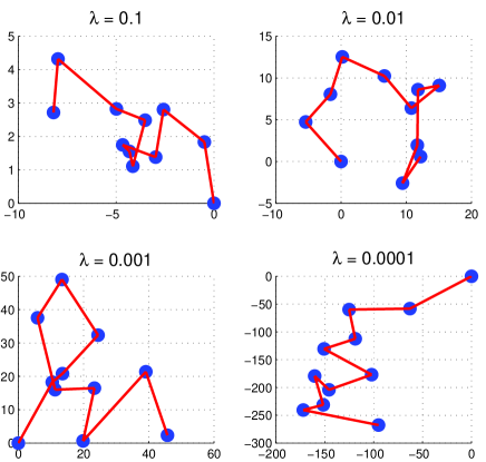
Under the proposed model, different mobility patterns can be captured by choosing different ’s. Larger statistically implies that the transition lengths are shorter. This further implies that the movement direction switch rates are higher. These mobility parameters may be appropriate for mobile users walking and shopping in a city, for example. In contrast, smaller statistically implies that the transition lengths are longer and the corresponding movement direction switch rates are lower. These mobility parameters may be appropriate for driving users, particularly those on the highways. This intuitive result can also be observed in Fig. 1, which shows sample traces of the proposed RWP model.
III Stochastic properties of the Proposed RWP mobility model
In this section, we first study the various stochastic properties of the proposed RWP mobility model. Stochastic properties of interests include transition length, transition time, direction switch rate, and the spatial node distribution. We then perform simulation to compare the proposed RWP mobility model to the classical RWP mobility model and a synthetic Levy Walk model proposed in [6], which is constructed from real mobility trajectories.
III-A Transition length
We define transition length as the Euclidean distance between two successive waypoints. In the proposed model, the transition lengths can be described by a stochastic process where are i.i.d. Rayleigh distributed with
| (2) |
Note that the transition lengths are not i.i.d. in the classical RWP mobility model. Indeed, a node currently located near the border of the finite domain tends to have a longer transition length while a node located around the center of the finite domain statistically has a shorter transition length for the next movement period. As a result, it is difficult to obtain the probability distribution for each random transition length.
Nevertheless, the random waypoints are i.i.d. in the classical RWP mobility model, which is obvious since they are selected uniformly from a finite domain and independently over movement periods. This property forms the basis for the analysis of the classical RWP mobility model (see, e.g., [5, 25]). In contrast, the waypoints in our proposed model are not i.i.d. but form a Markov process.
III-B Transition time
We define transition time as the time a node spends during the movement between two successive waypoints. We denote by the transition time for the movement period . Then where we omit the period index since are i.i.d.. Denote as the range of the random velocity . Given any velocity distribution , the probability distribution of is given as follows.
Proposition 1.
The cdf of the random transition time is given by
| (3) |
The proof of Prop. 3 is omitted for brevity. As a specific application of Prop. 3, the following corollary gives closed form expressions for transition times under two types of velocity distributions.
Corollary 1.
-
1.
If where is a positive constant, the pdf of transition time is
(4) -
2.
If is uniformly distributed on , the pdf of transition time is
(5) where is non-increasing, and .
III-C Direction switch rate
In this subsection, we study the direction switch rate, which is the inverse of the time between two direction changes and thus characterizes the frequency of direction change and is also a mobility parameter of interest [5]. To this end, we first introduce the period time, the time a node spends between two successive waypoints. In particular, period time is the sum of the pause time and the transition time, i.e., , where denotes the random pause time. Then the direction switch rate denoted by is defined to be the inverse of the period time: , whose probability distribution is described in the following proposition.
Proposition 2.
The cdf of the direction switch rate is given by
| (9) |
where denotes the range of the random pause time.
III-D Spatial node distribution
In this subsection, we study the spatial node distribution. To this end, let and be two successive waypoints. Given , we are interested in the probability that the moving node resides in some measurable set during the movement from to . We first derive the spatial node distribution given in the following theorem with the assumption that the mobile node does not have pause time.
Theorem 1.
Assume that , and that is at the origin. Then the spatial node distribution between and is characterized by the pdf given by
| (10) |
Proof.
See Appendix -A. ∎
The physical interpretation of is as follows. Let be a small area around the point given in polar coordinate. Then the probability that the moving node resides in some measurable set during the movement from to is approximately given by
| (11) |
where denotes the area of the set . Also, as noted in the proof in Appendix -A, can be regarded as the ratio of the expected proportion of transition time in the set to .
Now let us consider the case where the mobile node has random pause time , characterized by the probability measure . In this case, the spatial node distribution is given in the following theorem.
Theorem 2.
Assume that is at the origin. Then the spatial node distribution between and is characterized by the pdf :
| (12) |
where is the expected proportion of transition time from to .
Proof.
Note that the pause time is independent of both and . Besides, the non-static probability is the expected proportion of the time that the node is moving, i.e.,
| (13) |
The pdf is the weighted superposition of two independent components as [27]:
| (14) |
where is the spatial node distribution without pause time and is given in Theorem 10 , and denotes the spatial distribution of the waypoint and is given in Lemma 36. Plugging and into (14), the expression (12) follows. ∎
III-E Model comparison
In this section, we perform simulations to study the difference between the proposed RWP mobility model and the classical one. For validation, we also compare them to a synthetic truncated Levy walk model [6], which is constructed from real mobility trajectories. Thus, we indirectly compare the two RWP mobility models to real human walks. In the truncated Levy walk model, transition lengths have an inverse power-law distribution: . The pause times also have an inverse power-law distribution: .
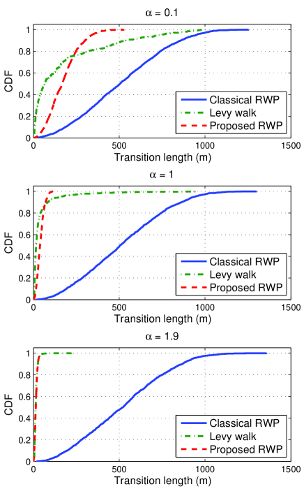
We simulate the movement of a mobile node under the three mobility models, respectively. The simulation area is a 10001000 grid.111Note that, though the proposed RWP mobility model is defined on the entire plane for analytical tractability, in a simulation one has to deal with the boundary issue. Here we use reflection method. Since the main assumption in the proposed model is the Rayleigh distributed transition lengths, we first compare the statistics of transition lengths under the three mobility models. The results are shown in Fig. 2, where is chosen such that the proposed RWP mobility model has the same mean transition length as that of Levy walk model. As shown in Fig. 2, transition lengths of the classical RWP mobility model are statistically much larger than those of Levy walk model. In contrast, transition lengths of the proposed RWP mobility model match those of Levy walk model better, especially in the low transition length regime. However, the proposed RWP mobility model lacks the heavy tail characteristic of the Levy walk model. This mismatch in the high transition length regime gradually diminishes as increases.
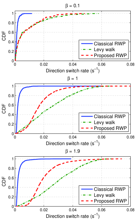
We next compare the statistics of direction switch rate under the 3 mobility models. The results are shown in Fig. 3, where is chosen such that the proposed RWP mobility model has the same mean transition length as that of Levy walk model. The pause time distribution used in the 2 RWP mobility models are the same power-law distribution as that used for pause time distribution in the Levy walk model. As expected, the classical RWP mobility model has much lower direction switch rate in all the 3 subplots than the Levy walk model. In contrast, the difference in direction switch rate between the proposed RWP mobility model and Levy walk model is moderate when is large. When is small, e.g., , the statistics of the direction switch rate of the proposed RWP mobility model are almost indistinguishable from those of the Levy walk model.
The above comparison shows that the proposed RWP model is more flexible for mobility simulation in future cellular networks which have ever-smaller cells than the classical RWP model. In particular, some aspects of the proposed RWP model can be directly or indirectly fitted using traces, while the classical RWP model is fixed. Nevertheless, the comparison does not imply that the statistical difference between the proposed RWP and Levy walk model are non-significant. Also, we do not claim that the proposed RWP model can fully represent human walks. Also, human walks are not Levy walks even though the Levy walk model is constructed from real mobility trajectories. Indeed, human walks have complex temporal and spatial correlations and its nature has not yet been fully understood [7]. It is fair to say that none of the existing mobility models can fully represent human walks.
Note that though many real mobility trajectories show that transition lengths of human walks seem to have an inverse power-law distribution, we do not choose it to model the transition lengths in our proposed RWP mobility model. The reason is that the mean transition length under inverse power-law distribution is infinite. This will cause analytical problems, e.g., the expected number of handovers in a movement period becomes infinite. Nevertheless, the analysis in this paper can be readily extended to any other transition length distribution which has finite mean.
IV Applications to Hexagonal Modeled Cellular Networks
In this and the next section, we study the impact of mobility on important cellular network parameters, particularly handover rate and sojourn time, using the proposed RWP mobility model. We focus on hexagonal cellular networks in this section.
IV-A Handover Rate
We assume the typical mobile user is located at the origin. Then the expected number of handovers during one movement period can be computed as
| (15) |
where is the probability distribution of the waypoint density given in Lemma 36 and denotes the area covered by the -th layer neighbouring cells. Now we formally define the handover rate.
Definition 1.
The handover rate is defined as the expected number of handovers during one movement period divided by the expected period time. Mathematically, handover rate is given by .
Note that where has been given in Prop. 3 and can be determined from the pause time distribution. However, exact computation of by (15) is tedious. Thus, we propose the following approximation formula
| (16) |
where with being the hexagonal cell size. In other words, we approximate the -th neighbouring layer by a ring with inner radius and outer radius . This approximation captures the essence of (15) and allows us to derive closed form results on and the corresponding lower and upper bounds.
Proposition 3.
Let be the side length of the hexagonal cell and the mobility parameter. The approximation of the expected number of handovers during one movement period is given by
| (17) |
and is bounded as where
| (18) | ||||
| (19) |
Moreover, the difference between the upper bound and lower bound is a strictly increasing function of and is within the range . In particular, , and .
Proof.
See Appendix -B. ∎
Using Prop. 3, the approximate handover rate can be computed as and is bounded as , where . As the size of the cells in cellular networks becomes smaller, higher handover rates are expected. In this regard, it is interesting to examine the asymptotic property of handover rate as in Corollary 20.
Corollary 2.
Assume that any of the following asymptotic conditions holds: 1) with fixed ; 2) with fixed ; 3) . Then the asymptotic approximate handover rate is given by
| (20) |
Though derivation by (15) is not tractable, the exact handover rate in hexagonal model can be obtained using a generalized solution of Buffon’s needle [34] as in the following Proposition.
Proposition 4.
Let be the side length of the hexagonal cell and the mobility parameter. The expected number of handovers during one movement period is given by
| (21) |
The handover rate is then given by
| (22) |
Proof.
See Appendix -C. ∎
We remark that the insights obtained by either approximate or exact approach are the same. Let us consider the simplified RWP mobility model where the mobile nodes do not have pause time and constant velocity, i.e., , the asymptotic handover rate in Corollary 20 can be further simplified as
| (23) |
and the exact handover rate is given by
| (24) |
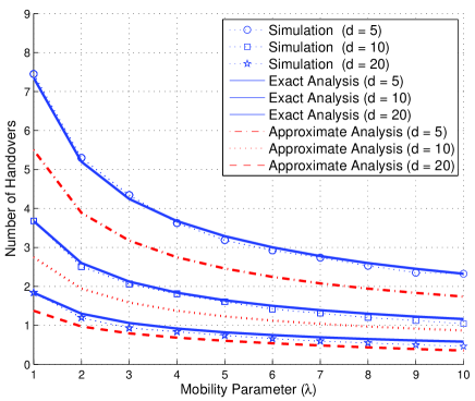
which is consistent with the one given in [35]. Note that the hexagonal cell size is given by in hexagonal tiling. So (23) can be written as . Similarly, the exact method yields . Both results imply that handover rate is inversely proportional to the square root of cell size . In other words, if we deploy more small cells and increase the BS density say by 4 times in current cellular network, we would expect the handover rate to be roughly increased by 2 times. Interestingly, the mobility parameter does not play a role, while the velocity and the cell size affect the handover rate in a trade-off manner. Fig. 4 compares the number of handovers obtained by simulation to the counterparts evaluated by analytic formula (17) and (21) respectively. It is shown that the exact analytic result closely matches the simulation while the approximation approach tends to underestimate the real number of handovers.
IV-B Sojourn Time
Sojourn time is defined as the expected duration that the mobile node stays within a particular serving cell. For brevity, we only consider the simplified RWP mobility model where the mobile nodes do not have pause time and constant velocity, i.e., . Then sojourn time in any cell with coverage area can be computed as
| (25) |
where is the probability distribution of the spatial node density given in Theorem 10. For brevity, we only focus on the sojourn time in the cell where the connection is initiated during one movement period in the sequel.
Assuming the mobile node is co-located with its currently associated BS at the origin, the sojourn time can be computed as
| (26) |
where . However, no closed form result is available for (26), though it can be evaluated using numerical methods. We provide explicit formulas for the lower and upper bounds of (26) in Prop. 5, whose proof is omitted for brevity.
Proposition 5.
The sojourn time can be bounded as where
| (27) | |||
| (28) |
Assuming that is finite222This is true for both the case with constant velocity and the case with uniformly distributed velocity on , as shown in Section III-B., tends to since both the lower bound and upper bound tend to as . This is an intuitive result. So cellular networks with small cells need to be equipped with fast algorithms. Otherwise, other handover strategies may be needed if the sojourn time in a cell is shorter than the time needed to complete the handover procedure. The analysis of the impact of mobility parameter is more involved. To obtain insight, consider the constant velocity case which yields the following result.
Proposition 6.
Assume that . Then as , sojourn time , where is a constant.
Proof.
See Appendix -D. ∎
From Prop. 6, we observe the interesting fact that sojourn time converges to as the mobility parameter goes to zero. Then what matters is the velocity: Sojourn time is inversely proportional to the velocity. Also, we can express as where recall that is the hexagonal cell size. This shows that sojourn time is proportional to the square root of cell size, which is contrary to the asymptotic result for handover rate.
V Applications to Poisson-Voronoi Modeled Cellular Networks
In this subsection, we apply the proposed RWP mobility model to analyze handover rate and sojourn time in cellular networks modeled by Poisson-Voronoi tessellation [36, 32]. We first give a brief description on Poisson-Voronoi tessellation. Consider a locally finite set of points , referred to as nuclei. The Voronoi cell of point with respect to is defined as
Let be the Dirac measure at , i.e., for , if , and otherwise. Then the spatial point process can be written as , and the Poisson-Voronoi tessellation is defined as follows [36].
Definition 2.
For a spatial Poisson point process on , the union of the associated Voronoi cells, i.e., , is called Poisson-Voronoi tessellation.
In cellular networks modeled by a Poisson-Voronoi tessellation, the BSs are the nuclei distributed according to some PPP in . Besides, each BS serves mobile users which are located within its Voronoi cell . The latter assumption is equivalent to the hypothesis of the nearest BS association strategy. In the sequel, we also assume that the PPP modeling the BS positions is homogeneous and its intensity is denoted by .
V-A Handover Rate
Assume that the mobile node is located at the origin and let and be two successive waypoints. Conditioned on the position of and a given realization of the Poisson-Voronoi tessellation, the number of handovers equals the number of intersections of the segment and the boundary of the Poisson-Voronoi tessellation. Then we can obtain the expected number of handovers by averaging over the spatial distribution of and the distribution of Poisson-Voronoi tessellation. This is the main idea used in proving Prop. 30.
Proposition 7.
Let be the intensity of the homogeneously PPP distributed BSs and the mobility parameter. The expected number of handovers during one movement period is given by
| (29) |
The handover rate is then given by
| (30) |
Proof.
See Appendix -E. ∎
If we assume no pause time and constant velocity , in Prop. 30 can be simplified as
| (31) |
which is consistent with the one given in [37]. In Poisson-Voronoi tessellation with the nuclei being homogeneous PPP of intensity , the expected value of the size of a typical Voronoi cell is given by [29], where is the typical cell and denotes the area of . So if we assume no pause time and constant velocity , in Prop. 30 can be simplified as which implies that the handover rate is inversely proportional to the square root of the cell size. This is consistent with the results in the hexagonal model.
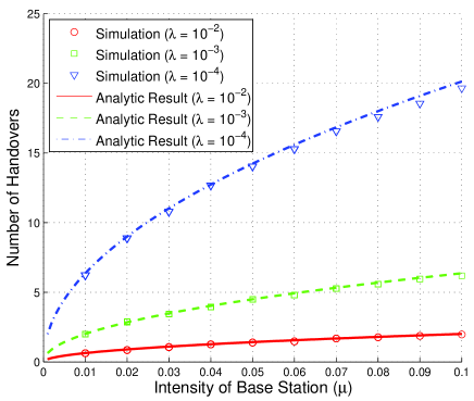
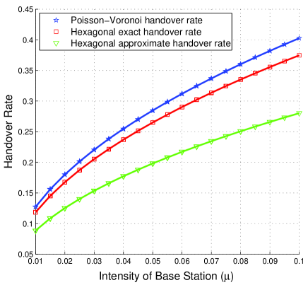
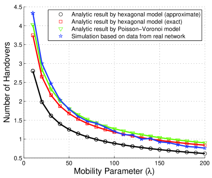
Fig. 5 illustrates that the analytical result (29) matches the simulation result quite well. Also, we compare the handover rate of Poisson-Voronoi model, exact and approximate handover rate of hexagonal model in Fig. 6 as a function BS intensity. They all indicate that handover rate grows linearly with the square root of the BS’s intensity . We further evaluate the three types of analytic results on handover, i.e., Prop. 3, Prop. 22 and 30 by simulating the proposed RWP mobility model using the real-world data of macro-BS deployment in a cellular network, provided by a major service provider. Recall that we assume each BS serves the mobile users located within its Voronoi cell. A handover occurs when the mobile crosses the cell boundary. Thus, only the BS location data are relevant in the simulation. There are 400 BSs which are distributed in a relatively flat urban area. These 400 BSs roughly occupy a 10590 km area. We normalize the network size to be 11. So in the Poisson-Voronoi model, while the side length in hexagonal model is determined through . The results are shown in Fig. 7. It can be seen that the Poisson-Voronoi model is about as accurate as the hexagonal model in predicting the number of handovers. Meanwhile, the approximate analytic result underestimates the number of handovers.
V-B Sojourn Time
Unlike the hexagonal model, (25) is not sufficient for computing the sojourn time in Poisson-Voronoi tessellation modeled cellular networks. Indeed, assuming that the mobile user is located at the origin, the sojourn time in the cell involves an additional source of randomness - the Poisson-Voronoi tessellation. So even averaging over the spatial node distribution sojourn time is still a random variable. In the sequel, we aim to characterize the probability distribution of this sojourn time. To this end, we first introduce the concept of contact distribution. Consider a random closed set and a convex compact test set containing the origin . Then the contact distribution is defined as [29]
| (32) |
In this paper, we are particularly interested in a special case: the linear contact distribution function with the test set being a segment of unit length . Since Poisson-Voronoi tessellation is isotropic, the orientation of this segment is not important. For Poisson-Voronoi tessellation modeled cellular network, the random closed set of interest is the union of all cell boundaries , where denotes the boundary of the cell .
With a slight abuse of notation, let denote the Voronoi cell containing the origin . We can further simplify as follows:
| (33) |
The last equality follows because 1) the origin is contained in the interior of almost surely and thus where , and 2) the event is equivalent to that . Now we are in a position to characterize the sojourn time .
Proposition 8.
Let be the intensity of the homogeneously PPP distributed BSs and the mobility parameter. The pdf of sojourn time is given by
| (34) |
where is the expected transition time, and is given by
| (35) |
where with , and , and .
Proof.
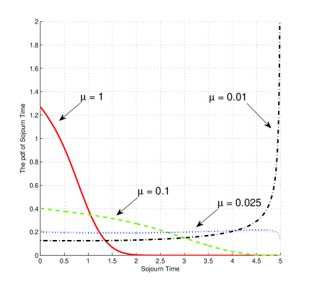
Using the previous results for expected transition time, the pdf of the sojourn time under different velocity distributions can be derived from Prop. 8. Note that the distribution of the sojourn time is instrumental in studying the ping-pong behavior for mobility enhancement in cellular networks [3]. Though a closed form expression is not available, the pdf of the sojourn time given in Proposition 8 only involves a double integral, which is tractable for efficient numerical evaluation. We plot the pdf of sojourn time in Fig. 8 for illustration. As expected, the smaller is, the more likely the mobile node stays longer within the cell. This is intuitive since a smaller implies larger cell sizes on average. As a result, it is less likely that the mobile node would move out of the cell.
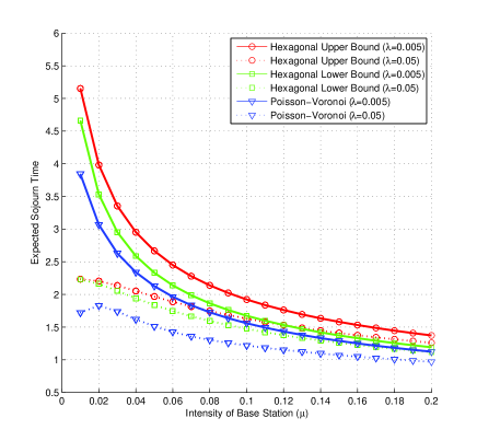
We also compare the analytic result about sojourn time in the Poisson-Voronoi model to its deterministic counterpart in the hexagonal model in Fig. 9. It is shown that the analytic result in the Poisson-Voronoi model is more conservative and yields smaller mean sojourn times than its counterpart in the hexagonal model. Besides, we can see that the upper and lower bounds of the sojourn time in hexagonal model are pretty tight.
VI Conclusions and Future Work
In this paper, we study the critical mobility issue in cellular networks. To this end, we first propose a tractable RWP mobility model defined on the entire plane. The various properties of the mobility model are carefully studied and simple analytical expressions are obtained. Then we utilize this tractable mobility model to analyze the handover rate and sojourn time in cellular networks. The analysis is carried out for cellular networks under both hexagonal and Poisson-Voronoi models. We derive closed form expressions and/or bounds for the performance metrics in question. These analytical results are instrumental for mobility management in cellular networks.
Note that the proposed RWP mobility model represents the real movement of mobile nodes in a simplified manner. Thus, it does not capture some other mobility characteristics such as temporal and spatial dependency of the mobility pattern. It is desirable to extend the current model further to incorporate these extra mobility characteristics while maintaining a certain degree of tractability. It would be rather interesting (and challenging) to characterize the intuitive tradeoff between the complexity and tractability of the mobility models. Besides, it is also interesting to evaluate the performance of the many wireless protocols by applying the proposed tractable model in theory and/or simulation.
Acknowledgment
The authors would like to thank the anonymous reviewers for their valuable comments and suggestions, which helped the authors significantly improve the quality of the paper.
-A Proof of Theorem 10
We first derive the pdf of the random waypoint as follows:
This result is summarized in Lemma 36 for ease of reference.
Lemma 1.
Given is at the origin, the pdf of the random waypoint is given by
| (36) |
We next derive the pdf of the spatial node distribution. The main technique of the following proof is inspired by [26], which is also adopted in [25]. Consider a small set located at . Let denote the vector and . Then the pdf of the spatial node distribution can be interpreted as the ratio of the expected proportion of transition time in the set to the area , i.e.,
| (37) |
where the second equality follows from the independence of and the waypoints. Note that
| (38) |
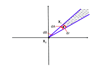
where denotes the length of the small intersection if intersects , and we apply Lemma 36 in the second equality in (38). The first equality in (38) can be explained through Fig. 10 as follows. The intersection of is if is in the shaded area and otherwise. Noting that the probability of the event that is in the shaded area is , we have
| (39) |
This and give the desired equality. So
| (40) |
where we use the result that in the last equality. This completes the proof.
-B Proof of Proposition 3
From Lemma 36, . We compute as follows.
Substituting , we obtain
Then the lower bound is derived as follows.
The upper bound can be derived in a similar manner. For the remaining proof, denote . Note that . Then the difference can be compactly written as which we denote by . We claim is strictly decreasing when . To see this, define whose derivative is “” which is strictly negative when , implying is strictly decreasing when . Meanwhile, . So when . Now it is clear that the derivative of given by is strictly negative when . Thus, is strictly decreasing when . Besides,
The desired results follow by further observing is a strictly increasing continuous function of .
-C Proof of Proposition 22
We use (generalized) argument for Buffon’s needle problem in this proof. Consider the typical node located in area of size and cell boundaries of length . Then the probability that this node crosses the small boundary within a small time interval is , where is uniformly distributed on (following from our mobility model) and thus . So the probability that this node crosses is . Thus, conditioned on moving, the handover rate
Correspondingly, and .
-D Proof of Proposition 6
Applying the general expression (26) for yields
which equals
| (41) |
where are a pair of constants in the region , and in the last equality we use derived for constant velocity case in Section III, and mean value theorem for integrals. Then, Next we give bounds on the constant . Using the bounds given in Prop. 5,
| (42) |
Similarly, . Since these bounds are strict, we conclude that .
-E Proof of Proposition 30
This proposition can be proved by following the proof of Prop. 22. Nevertheless, we provide an alternative proof here. To this end, we first introduce some terminologies for ease of exposition. Consider the set consisting of arbitrary distinct points in on . Without loss of generality, we assume . Then if the intersection then is called a ()-facet. Now let be the set of all configurations . That is, the intersection of the Voronoi cells associated with any configuration is a -facet. For each configuration , we associate a point called “centroid” such that for all , . Note that there are several degrees of freedom in choosing the centroids. We refer to [36] for more details.
Consider the intersection of the Poisson-Voronoi tessellation with a fixed line . Without loss of generality, we assume that contains the origin. Then the nonempty sectional cells satisfy that (i) , and (ii) where denotes the relative interior [36]. So the sectional cells constitute a tessellation of , denoted by . Now consider the intersection which can be either empty or a singleton. Clearly, is the -facet of tessellation if is nonempty. Now let which parametrizes the -facets of . Then the intensity of the -facets of is well defined as
| (43) |
where is indicator function taking value if the event in its argument is true and otherwise, is the centroid of the -facets of , is any arbitrary Borel set and is the volume of with respect to .
Without loss of generality, assume that is at the origin. Let be the line containing and , and the interval . Then conditioned on the next waypoint , the expected number of handovers can be computed as
| (44) | ||||
| (45) |
where in (44) denotes the boundary of the cell . The equality in (44) follows by choosing the centroids as follows: for any , choose the singleton as the centroid of the -facets of . The equality in (45) follows from (43). The last equality follows since for Poisson-Voronoi tessellation with intensity [36]. Then handover rate can be computed as follows:
| (46) | ||||
| (47) |
where in (46) we use Lemma 36, and in (47) we apply the result that for . Plugging yields the desired results.
References
- [1] T. Camp, J. Boleng, and V. Davies, “A survey of mobility models for ad hoc network research,” Wireless Communications and Mobile Computing, vol. 2, no. 5, pp. 483–502, 2002.
- [2] I. Akyildiz, J. Mcnair, J. Ho, H. Uzunalioglu, and W. Wang, “Mobility management in next-generation wireless systems,” Proceedings of the IEEE, vol. 87, no. 8, pp. 1347–1384, August 1999.
- [3] “Evolved universal terrestrial radio access (E-UTRA): Mobility enhancements in heterogeneous networks,” 3GPP TR 36.8de V0.0.1, Technical Report, May 2011.
- [4] D. Johnson and D. Maltz, “Dynamic source routing in ad hoc wireless networks,” Mobile Computing, pp. 153–181, 1996.
- [5] C. Bettstetter, H. Hartenstein, and X. Pérez-Costa, “Stochastic properties of the random waypoint mobility model,” Wireless Networks, vol. 10, no. 5, pp. 555–567, September 2004.
- [6] I. Rhee, M. Shin, S. Hong, K. Lee, S. Kim, and S. Chong, “On the levy-walk nature of human mobility,” IEEE/ACM Transactions on Networking, vol. 19, no. 3, pp. 630–643, 2011.
- [7] M. Gonzalez, C. Hidalgo, and A. Barabási, “Understanding individual human mobility patterns,” Nature, vol. 453, no. 7196, pp. 779–782, 2008.
- [8] C. Song, T. Koren, P. Wang, and A. Barabási, “Modelling the scaling properties of human mobility,” Nature Physics, vol. 6, no. 10, pp. 818–823, 2010.
- [9] P. J. Fleming, A. L. Stolyar, and B. Simon, “Closed-form expressions for other-cell interference in cellular CDMA,” Technical Report 116, Univ. of Colorado at Boulder, December 1997. [Online]. Available: http://ccm.ucdenver.edu/reports/
- [10] T. X. Brown, “Cellular performance bounds via shotgun cellular systems,” IEEE Journal on Selected Areas in Communications, vol. 18, no. 11, pp. 2443 – 55, November 2000.
- [11] J. Andrews, F. Baccelli, and R. Ganti, “A tractable approach to coverage and rate in cellular networks,” IEEE Transactions on Communications, vol. 59, no. 11, pp. 3122 –3134, November 2011.
- [12] E. Royer, P. Melliar-Smith, and L. Moser, “An analysis of the optimum node density for ad hoc mobile networks,” in Proceedings of IEEE International Conference on Communications, vol. 3. IEEE, 2001, pp. 857–861.
- [13] P. Nain, D. Towsley, B. Liu, and Z. Liu, “Properties of random direction models,” in Proceedings of IEEE INFOCOM, vol. 3. IEEE, 2005, pp. 1897–1907.
- [14] X. Hong, M. Gerla, G. Pei, and C. Chiang, “A group mobility model for ad hoc wireless networks,” in Proceedings of the 2nd ACM international workshop on Modeling, analysis and simulation of wireless and mobile systems. ACM, 1999, pp. 53–60.
- [15] A. Jardosh, E. Belding-Royer, K. Almeroth, and S. Suri, “Towards realistic mobility models for mobile ad hoc networks,” in Proceedings of ACM Mobicom. ACM, 2003, pp. 217–229.
- [16] M. Musolesi, S. Hailes, and C. Mascolo, “An ad hoc mobility model founded on social network theory,” in Proceedings of the 7th ACM international symposium on Modeling, analysis and simulation of wireless and mobile systems. ACM, 2004, pp. 20–24.
- [17] A. Saha and D. Johnson, “Modeling mobility for vehicular ad-hoc networks,” in Proceedings of the 1st ACM international workshop on Vehicular ad hoc networks. ACM, 2004, pp. 91–92.
- [18] W. Hsu, K. Merchant, H. Shu, C. Hsu, and A. Helmy, “Weighted waypoint mobility model and its impact on ad hoc networks,” ACM SIGMOBILE Mobile Computing and Communications Review, vol. 9, no. 1, pp. 59–63, 2005.
- [19] M. McNett and G. M. Voelker, “Access and mobility of wireless pda users,” ACM SIGMOBILE Mobile Computing and Communications Review, vol. 9, no. 2, pp. 40–55, 2005.
- [20] M. Kim, D. Kotz, and S. Kim, “Extracting a mobility model from real user traces,” in Proceedings of IEEE Infocom, vol. 6. Citeseer, 2006, pp. 1–13.
- [21] K. Lee, S. Hong, S. Kim, I. Rhee, and S. Chong, “SLAW: A new mobility model for human walks,” in Proceedings of IEEE Infocom. IEEE, 2009, pp. 855–863.
- [22] W. Hsu, T. Spyropoulos, K. Psounis, and A. Helmy, “Modeling spatial and temporal dependencies of user mobility in wireless mobile networks,” IEEE/ACM Transactions on Networking, vol. 17, no. 5, pp. 1564–1577, 2009.
- [23] N. Aschenbruck, A. Munjal, and T. Camp, “Trace-based mobility modeling for multi-hop wireless networks,” Computer Communications, vol. 34, no. 6, pp. 704–714, 2011.
- [24] E. Cho, S. A. Myers, and J. Leskovec, “Friendship and mobility: user movement in location-based social networks,” in Proceedings of the 17th ACM SIGKDD international conference on Knowledge discovery and data mining. ACM, 2011, pp. 1082–1090.
- [25] E. Hyytia, P. Lassila, and J. Virtamo, “Spatial node distribution of the random waypoint mobility model with applications,” IEEE Transactions on Mobile Computing, pp. 680–694, June 2006.
- [26] C. Bettstetter, G. Resta, and P. Santi, “The node distribution of the random waypoint mobility model for wireless ad hoc networks,” IEEE Transactions on Mobile Computing, pp. 257–269, September 2003.
- [27] G. Resta and P. Santi, “An analysis of the node spatial distribution of the random waypoint mobility model for ad hoc networks,” in Proceedings of the second ACM international workshop on Principles of mobile computing. ACM, 2002, pp. 44–50.
- [28] E. Hyytiä and J. Virtamo, “Random waypoint mobility model in cellular networks,” Wireless Networks, vol. 13, no. 2, pp. 177–188, 2007.
- [29] D. Stoyan, W. S. Kendall, and J. Mecke, Stochastic Geometry and its Applications, 2nd ed. John Wiley and Sons, 1995.
- [30] M. Haenggi, Stochastic Geometry for Wireless Networks. Cambridge University Publishers, 2012.
- [31] M. Haenggi, J. Andrews, F. Baccelli, O. Dousse, and M. Franceschetti, “Stochastic geometry and random graphs for the analysis and design of wireless networks,” IEEE Journal on Selected Areas in Communications, vol. 27, no. 7, pp. 1029–1046, September 2009.
- [32] F. Baccelli and B. Blaszczyszyn, Stochastic Geometry and Wireless Networks - Part I: Theory. Now Publishers Inc, 2009.
- [33] F. Baccelli and S. Zuyev, “Stochastic geometry models of mobile communication networks,” Frontiers in Queueing, pp. 227–243, 1997.
- [34] L. Schroeder, “Buffon’s needle problem: An exciting application of many mathematical concepts,” Mathematics Teacher, vol. 67, no. 2, pp. 183–186, 1974.
- [35] V. Casares-Giner, V. Pla, and P. Escalle-García, “Mobility models for mobility management,” Network performance engineering, pp. 716–745, 2011.
- [36] J. Møller, Lectures on random Voronoi tessellations. Springer-Verlag, 1994, vol. 87.
- [37] F. Baccelli and S. Zuyev, “Poisson-Voronoi spanning trees with applications to the optimization of communication networks,” Operations Research, pp. 619–631, 1999.
- [38] L. Muche, “Contact and chord length distribution functions of the Poisson-Voronoi tessellation in high dimensions,” Advances in Applied Probability, vol. 42, no. 1, pp. 48–68, 2010.