Vision-Based Cooperative Estimation of Averaged 3D Target Pose under Imperfect Visibility
Abstract
This paper investigates vision-based cooperative estimation of a 3D target object pose for visual sensor networks. In our previous works, we presented an estimation mechanism called networked visual motion observer achieving averaging of local pose estimates in real time. This paper extends the mechanism so that it works even in the presence of cameras not viewing the target due to the limited view angles and obstructions in order to fully take advantage of the networked vision system. Then, we analyze the averaging performance attained by the proposed mechanism and clarify a relation between the feedback gains in the algorithm and the performance. Finally, we demonstrate the effectiveness of the algorithm through simulation.
keywords:
Cooperative estimation, Distributed averaging, Visual sensor networks1 Introduction
Driven by technological innovations of smart wearable vision cameras, a networked vision system consisting of spatially distributed smart cameras emerges as a new challenging application field of the visual feedback control and estimation (Song et al. (2011); Tron and Vidal (2011)). The vision system called visual sensor network brings in some potential advantages over a single camera system such as: (i) accurate estimation by integrating rich information, (ii) tolerance against obstructions, misdetection in image processing and sensor failures and (iii) wide vision and elimination of blind areas by fusing images of a scene from a variety of viewpoints. Due to their nature, the visual sensor networks are expected as a component of sustainable infrastructures.
Fusion of control techniques and visual information has a long history, which is well summarized by Chaumette and Hutchinson (2006, 2007); Ma et al. (2004). Among a variety of estimation/control problems addressed in the literature, this paper investigates a vision-based estimation problem of 3D target object motion as in Aguiar and Hespanha (2009); Dani et al. (2011); Fujita et al. (2007). While most of the above works consider estimation by a single or centralized vision system, we consider a cooperative estimation problem for visual sensor networks. In particular, we confine our focus to a 3D pose estimation problem of a moving target object addressed by Fujita et al. (2007), where the authors present a real-time vision-based observer called visual motion observer. Namely, we investigate cooperative estimation of a target object pose via distributed processing.
Cooperative estimation for sensor networks has been addressed e.g. in Olfati-Saber (2007); Freeman et al. (2006). The main objective of these researches is averaging the local measurements or local estimates among sensors in a distributed fashion to improve estimation accuracy. For this purpose, most of the works utilize the consensus protocol (Olfati-Saber et al. (2007)) in the update procedure of the local estimates. However, the consensus protocol is not applicable to the full 3D pose estimation problem as pointed out by Tron and Vidal (2011), since the object’s pose takes values in a non-Euclidean space.
Meanwhile, Tron and Vidal (2011); Sarlette and Sepulchre (2009) present a distributed averaging algorithm on matrix manifolds. However, applying them to cooperative estimation requires a lot of averaging iterations at each update of the estimate and hence they cannot deal with the case where the target motion is not slow. To overcome the problem, the authors presented a cooperative estimation mechanism called networked visual motion observer achieving distributed estimation of an object pose in real time (Hatanaka et al. (2011); Hatanaka and Fujita (2012)) by using a pose synchronization techniques in Hatanaka et al. (2012). However, Hatanaka et al. (2011); Hatanaka and Fujita (2012) assume that all the cameras capture the target object, which may spoil the advantage (iii) of the first paragraph of this section. Though running the algorithm only among the cameras viewing the target and broadcasting the estimates to the other cameras is an option, it is desirable to share an estimate without changing procedures of each camera in order to avoid such complicated task switches depending on the situation.
In this paper, we thus present a novel estimation mechanism which works in the presence of cameras not capturing the target due to limited view angles and obstructions. Then, we analyze the averaging performance attained by the proposed mechanism and clarify a relation between the tuning gains and the averaging performance. There, we prove that the conclusion of Hatanaka et al. (2011); Hatanaka and Fujita (2012) under the assumption of perfect visibility is also valid even in the case of imperfect visibility. Moreover, we demonstrate the effectiveness of the presented algorithm through simulation.
2 Problem Statement
2.1 Situation under Consideration
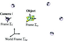
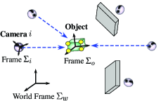
In this paper, we consider the situation where there are cameras with communication and computation capability and a single target object in 3 dimensional space as in the left figure of Fig. 1. Let the world frame, the -th camera frame and the object frame be denoted by , and , respectively. The objective of the networked vision system is to estimate the 3D pose of the object from visual measurements. Although the targets are possibly multiple in a practical situation, we confine our focus only to estimation of a single target since multiple objects case can be handled by just applying parallely the procedure for a single object to each object.
Unlike Hatanaka et al. (2011); Hatanaka and Fujita (2012), all the vision cameras are assumed to have visible region and some cameras do not capture the target object as depicted in the right figure of Fig. 1. Let us now denote the subset of all vision cameras viewing the target at time by and the rest of the cameras by .
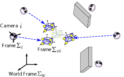
Suppose that the pose consistent with the visual measurement of each camera differs from camera to camera due to incomplete localization and parametric uncertainties of the cameras as depicted in Fig. 2. Then, the fictitious target with the pose consistent with the -th camera’s visual measurement is denoted by and its frame is by . Under such a situation, averaging the contaminated poses is a way to improve estimation accuracy (Olfati-Saber (2007); Tron and Vidal (2011)). In this paper, we thus address estimation of an average pose of objects in a distributed fashion.
2.2 Relative Rigid Body Motion
The position vector and the rotation matrix from -th camera frame to the world frame are denoted by and . The vector specifies the rotation axis and is the rotation angle. We use to denote . The notation is the operator such that , for the vector cross-product , i.e. is a skew-symmetric matrix. The notation denotes the inverse operator to .
The pair of the position and the orientation denoted by is called the pose of camera relative to the world frame . Similarly, we denote by the pose of object relative to the world frame . We also define the body velocity of camera relative to the world frame as , where and respectively represent the linear and angular velocities of the origin of relative to . Similarly, object ’s body velocity relative to is denoted by .
Throughout this paper, we use the following homogeneous representation of and .
| (5) |
Then, the body velocities and are simply given by and .
Let be the pose of relative to . Then, it is known that can be represented as . By using the body velocities and , the motion of the relative pose is written as
| (6) |
(Ma et al. (2004)). (6) is called relative rigid body motion.
2.3 Visual Measurement
In this subsection, we define visual measurements of each vision camera which is available for estimation. Unlike Hatanaka et al. (2011); Hatanaka and Fujita (2012), all the cameras in obtain no measurement. Now, we assume (i) all cameras are pinhole-type cameras, (ii) each target object has feature points and (iii) each camera can extract them from the vision data. The position vectors of object ’s -th feature point relative to and are denoted by and respectively. Using a transformation of the coordinates, we have , where and should be regarded with a slight abuse of notation as and .
Let the feature points of object on the image plane coordinate be the measurement of camera , which is given by the perspective projection (Ma et al. (2004)) as
| (10) |
with a focal length , where . In this paper, we assume that each camera knows the location of feature points . Then, the visual measurement depends only on the relative pose from (10) and . Fig. 3 shows the block diagram of the relative rigid body motion (6) with the camera model (10), where RRBM is the acronym of Relative Rigid Body Motion.

2.4 Communication Model
The cameras have communication capability with the neighboring cameras and form a network. The communication is modeled by a graph , . Namely, camera can get information from if . We also define the neighbor set of camera as
| (11) |
In this paper, we employ the following assumption on the graph .
Assumption 1
The communication graph is fixed, undirected and connected.
We also introduce some additional notations. Let be the set of all spanning trees over with a root and we consider an element . Let the path from to node along with be denoted by , where is the length of the path . We also define
for any and
| (12) | |||||
The meaning of these notations are given in Hatanaka and Fujita (2012).
2.5 Average on SE(3)
The objective of this paper is to present a cooperative estimation mechanism for the visual sensor networks producing an estimate close to an average of , even in the presence of vision cameras not capturing the target.
Let us now introduce the following mean on (Moakher (2002)) as an average of target poses .
| (13) |
where is defined for any as
| (14) | |||||
| (15) |
and is the Frobenius norm of matrix . Hereafter, we also use the notation .
3 Networked Visual Motion Observer
In this section, we introduce a cooperative estimation mechanism originally presented by Hatanaka et al. (2011). Here, we assume that the relative poses w.r.t neighbors are available for each camera .
3.1 Review of Previous Works
We first prepare a model of the rigid body motion (6) as
| (16) |
where is the estimate of the average . The input is to be designed so that approaches . Once is determined, the estimated visual measurement is computed by (10).
Let us now define the error between the estimate and the relative pose and its vector representation with
| (18) | |||||
| (19) |
It is shown by Fujita et al. (2007) that if the number of feature points is greater than or equal to 4, the estimation error vector can be approximately reconstructed by the visual measurement error as
| (20) |
In case of a single camera, Fujita et al. (2007) presents an input based on passivity of the estimation error system from to and the resulting estimation mechanism (16), (20) and is called visual motion observer. Then, the authors prove the estimate converges to the actual relative pose if .
Hatanaka et al. (2011) extended the results in Fujita et al. (2007) to the networked vision systems, where the following input to the model (16) was proposed.
| (21) |
with . The input consists of both visual feedback term and mutual feedback term inspired by pose synchronization in Hatanaka et al. (2012). The resulting networked estimation mechanism (16), (20) and (21) is named networked visual motion observer. Then, the paper analyzed the averaging performance attained by the proposed mechanism.
3.2 Networked Visual Motion Observer under Imperfect Visibility
In the presence of the cameras not capturing the target, cannot implement the visual feedback term in (21). We thus employ the following input instead of (21).
| (22) |
where if and otherwise. The total estimation mechanism is formulated as (16), (20) and the inputs (22) whose block diagram with respect to camera is illustrated in Fig. 4.
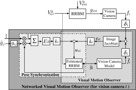
The input (22) for is the gradient decent algorithm on of the local objective function (Absil et al. (2008)), which means each camera in aims at leading its estimate to its neighbors’ estimates . On the other hand, the input for aims at leading to both of object pose and neighbors’ estimates. Meanwhile, the global objective is given by (13), which differs from the local objective functions. Thus, the closeness between the estimates and the global objective minimizer is not clear.
In the next section, we thus clarify the averaging performance. Although it is conjectured from its structure and demonstrated through simulation (http://www.fl.ctrl.titech.ac.jp/researches/movie_new/sim/sw_coopest.wmv) that the present mechanism works for a moving object, we will derive a theoretical result under the assumption that the target object is static (). The main reason to use this assumption is to assure time invariance of . Indeed, in case of the time varying , the global objective itself changes in time and it is necessary to find a metric evaluating the performance in order to conduct theoretical analysis, which is left as a future work of this paper.
4 Averaging Performance
In this section, we derive ultimate estimation accuracy of the average achieved by the presented mechanism assuming that the object is static (). Throughout this section, we use the following assumption.
Assumption 2
- (i)
-
The number of elements of is greater than or equal to () and there exists a pair such that and .
- (ii)
-
for all .
The item (i) is assumed just to avoid a meaningless problem such that all the poses in are equal under which it is straightforward to prove convergence of the estimates to the common pose by using the techniques presented by Hatanaka et al. (2012). The detailed discussions on validity of the assumption (ii) is shown in Hatanaka and Fujita (2012) but it is in general satisfied in the scenario of the beginning of Section 2.
4.1 Definition of Approximate Averaging
In this subsection, we introduce a notion of approximate averaging similarly to Hatanaka and Fujita (2012). For this purpose, we define parameters
and the following sets for any positive parameter .
Let us define -level averaging performance to be met by the estimates .
Definition 3
Given target poses and , the position estimates and orientation estimates are respectively said to achieve -level averaging performance, if there exists a finite such that
In case of , and indicate average estimation accuracy in the absence of the mutual feedback term of in (22) since the visual motion observer correctly estimates the static object pose . In the case, the parameter is an indicator of improvement of average estimation accuracy by inserting the mutual feedback term.
4.2 Averaging Performance Analysis
In this subsection, we state the main result of this paper. For this purpose, we first define a value
and a parameter strictly greater than . Then, we have the following lemma.
Lemma 4
We are now ready to state the main result of this section.
Theorem 5
Suppose the targets are static ( ) and the estimates are updated according to (16) and (22). Then, under Assumptions 1 and 2 and , if the initial estimates satisfy , for any , there exists a sufficiently small such that the position estimates achieve -level averaging performance and the orientation estimates achieve -level averaging performance with .
See Appendix B. Theorem 5 says that choosing the gains and such that is sufficiently small leads to a good averaging performance. The conclusion is the same as Hatanaka et al. (2011); Hatanaka and Fujita (2012) and hence the contribution of the theorem is to prove the statement is also valid even in the presence of the cameras not viewing the target. We also see an essential difference between the position and orientation estimates that the averaging performance on positions can be arbitrarily improved by choosing a sufficiently small but an offset associated with occurs for the orientation estimates.
5 Verification through simulation
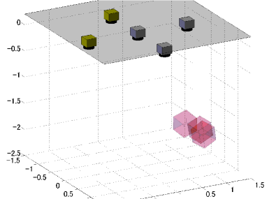
We finally demonstrate the effectiveness of the present algorithm through simulation. Here, we consider five pin-hole type cameras with focal length connected by the communication graph with . We identify the frame of camera 1 with the world frame and let and . Let only cameras (gray boxes in Fig. 6) capture the target, i.e. .
We set the configurations of target objects as . The red boxes in Fig. 6 represent the initial configuration of target objects and yellow boxes represent the cameras . Then, the average is given by .
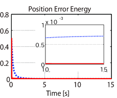
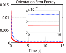
We run simulations with two different gains and from the initial condition and . Fig. 6 shows the time responses of the position estimation error energy
and orientation estimation error energy defined in (36), where the red solid curves illustrate the result for and the blue dashed curves that for . We see from both figures that the energies for the larger mutual feedback gain are smaller than those for , which implies that a large and hence a small achieves a good averaging performance as indicated by Theorem 5. Fig. 7 illustrates the time responses of the first element of orientation estimates of all cameras produced by the networked visual motion observer, where the red dash-dotted line represents the average. We also see from the figure that, while the estimate of camera 2 for is far from the average, all the estimates for approaches to it. However, we also confirm that an offset still occurs even in case of as indicated in Theorem 5.
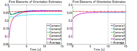
(Left: , Right )
6 Conclusion
In this paper, we have investigated a vision-based cooperative estimation problem of a 3D target object pose for visual sensor networks. In particular, we have extended the networked visual motion observer presented by Hatanaka et al. (2011) so that it works even in the presence of cameras not viewing the target due to the limited view angles and obstructions. Then, we have analyzed the averaging performance attained by the present mechanism. Finally, we have demonstrated the effectiveness of the present algorithm through simulation.
References
- Song et al. (2011) B. Song, C. Ding, A. Kamal, J. A. Farrell and A. Roy-Chowdhury. Distributed Camera Networks: Integrated Sensing and Analysis for Wide Area Scene Understanding. IEEE Signal Processing Magazine, volume 28, No. 3, pages 20–31, 2011.
- Tron and Vidal (2011) R. Tron and R. Vidal. Distributed Computer Vision Algorithms. IEEE Signal Processing Magazine, volume 28, No. 3, pages 32–45, 2011.
- Chaumette and Hutchinson (2006) F. Chaumette and S. Hutchinson. Visual Servo Control, Part I: Basic Approaches. IEEE Robotics and Automation Magazine, volume 13, No. 4, pages 82–90, 2006.
- Chaumette and Hutchinson (2007) F. Chaumette and S. Hutchinson. Visual Servo Control, Part II: Advanced Approaches. IEEE Robotics and Automation Magazine, volume 14, No. 1, pages 109–118, 2007.
- Ma et al. (2004) Y. Ma, S. Soatto, J. Kosecka and S. S. Sastry. An Invitation to 3-D Vision: From Images to Geometric Models. Springer-Verlag, 2004.
- Aguiar and Hespanha (2009) A. Aguiar and J. Hespanha. Robust Filtering for Deterministic Systems with Implicit Outputs. Systems and Control Letters, volume 58, No. 4, pages 263–270, 2009.
- Dani et al. (2011) A. P. Dani, Z. Kan, N. R. Fischer and W. E. Dixon. Structure of a Moving Object Using a Moving Camera: An Unknown Input Observer Approach. Proc. of the 50th IEEE Conference on Decision and Control, pages 5005–5010, 2011.
- Fujita et al. (2007) M. Fujita, H. Kawai and M. W. Spong. Passivity-based Dynamic Visual Feedback Control for Three Dimensional Target Tracking: Stability and L2-gain Performance Analysis. IEEE Trans. on Control Systems Technology, volume 15, No. 1, pages 40–52, 2007.
- Olfati-Saber (2007) R. Olfati-Saber. Distributed Kalman Filtering for Sensor Networks. Proc. of the 46th IEEE Conference on Decision and Control, pages 5492–5498, 2007.
- Freeman et al. (2006) R. A. Freeman, P. Yang, and K. M. Lynch. Stability and Convergence Properties of Dynamic Average Consensus Estimators. Proc. of the 45th IEEE Conference on Decision and Control, pages 398–403, 2006.
- Olfati-Saber et al. (2007) R. Olfati-Saber, J. A. Fax and R. M. Murray, Consensus and Cooperation in Networked Multi-Agent Systems. Proc. of the IEEE, volume 95, No. 1, pages 215–233, 2007.
- Sarlette and Sepulchre (2009) A. Sarlette and R. Sepulchre. Consensus Optimization on Manifolds. SIAM Journal on Control and Optimization, volume 48, No. 1, pages 56–76, 2009.
- Hatanaka et al. (2011) T. Hatanaka, K. Hirata and M. Fujita. Cooperative Estimation of 3D Target Object Motion via Networked Visual Motion Observers Proc. of the 50th IEEE Conference on Decision and Control, pages 4979-4984, 2011.
- Hatanaka and Fujita (2012) T. Hatanaka and M. Fujita. Cooperative Estimation of 3D Target Motion via Networked Visual Motion Observers. IEEE Trans. on Automatic Control, submitted, 2012 (Available at http://arxiv.org/abs/1107.5108).
- Hatanaka et al. (2012) T. Hatanaka, Y. Igarashi, M. Fujita and M. W. Spong. Passivity-based Pose Synchronization in Three Dimensions. IEEE Trans. on Automatic Control, volume 57, No. 2, pages 360–375, 2012.
- Olfati-Saber et al. (2007) R. Olfati-Saber, J. A. Fax and R. M. Murray. Consensus and Cooperation in Networked Multi-Agent Systems. Proc. of the IEEE, volume 95, No. 1, pages 215–233, 2007.
- Moakher (2002) M. Moakher. Means and Averaging in the Group of Rotations. SIAM Journal on Matrix Analysis and Applications, volume 24, No. 1, pages 1–16, 2002.
- Absil et al. (2008) P. A. Absil, R. Mahony and R. Sepulchre. Optimization Algorithms on Matrix Manifolds. Princeton Press, 2008.
- Chopra and Spong (2006) N. Chopra and M. W. Spong. Passivity-Based Control of Multi-Agent Systems. Advances in Robot Control: From Everyday Physics to Human-Like Movements, S. Kawamura and M. Svnin (eds.), pages 107–134, Springer, 2006.
Appendix A Proof of Lemma 4
In the proof, we use the following lemma.
Lemma 6 (Hatanaka et al. (2012))
For any matrices , the inequality
| (23) | |||||
holds, where and is the minimal eigenvalue of matrix .
Extracting the time evolution of the orientation estimates from (16) with (22) and transforming their coordinates from to as yields
| (24) | |||||
| (25) | |||||
which is independent of evolution of the position estimates.
Let us now consider the energy function
| (26) |
similarly to Lemma 1 in Hatanaka and Fujita (2012), where . The time derivative of along with the trajectories of (24) with (25) is given as
| (27) | |||||
where we use the relation . Substituting (25) into (27) yields
| (28) | |||||
From Lemma 6, (28) is rewritten as
where
The inequality holds from the definition of the index , and hence we obtain . Thus, the inequality
is true. From Assumption 2, we have and hence
| (29) |
Suppose now that . Then, if , is true from the definition of . On the other hand, in case of , we also have . Namely, the function never increases as long as an estimate satisfies . This implies that once the estimates enter
at a time, stays in the set for all subsequent time.
Let us now employ another energy function
| (30) | |||||
| (31) |
The function is continuous but it may not be differentiable on the region where an estimate satisfies . Except for the region, the time derivative of along with the trajectories of (24) is given by
| (32) |
We first consider
| (33) |
in the second term of . In case of , we have
Otherwise (), the term
has to appear in (33) under Assumption 1 and they are canceled. Thus, the inequality
holds and hence we obtain
| (34) |
Note that the equality of (34) can hold only if or since, otherwise, there must be a pair of such that and from Assumption 1.
Now, substituting (34) into (32) yields
We see from the inequality and the definition of that if there exists then . In addition, if , then the inequality (34) strictly holds and hence . Namely, the function is strictly decreasing except for the region where an estimate satisfies
| (35) |
Since the function is continuous despite of the event that an estimate goes across the region, the function decreases and the estimates enters at least once as long as the time interval
is bounded and the number of occurrences of the event (35) is finite. As proved above, if all the estimates enter once they have to stay there for all subsequent time.
Let us now define and by just replacing by . Then, all the above discussions hold true. Notice that every time an estimate goes across the region of (35), the estimate has to spend nonzero finite time in the region where from continuity of and . During the period, the function is strictly decreasing. Namely, if the event happens infinitely often, , which contradicts . The possibility that is unbounded is also excluded in the same way. This completes the proof.
Appendix B Proof of Theorem 5
In this paper, we prove only the orientation part since it is possible to prove the position part in the same way. The evolution of orientation estimates is described by (24) with (25).
We first define the energy function
| (36) |
and the sets
Then, we first prove the following lemma.
Lemma 7
The time derivative of along the trajectories of (24) and (25) is given by
| (37) | |||||
Substituting (25) into (37) yields
| (38) | |||||
We first consider the term . From Lemma 6, the following inequality holds.
| (39) | |||||
Assumption 1 implies that
(Hatanaka et al. (2012)). From Lemma 4, (39) is rewritten as
| (40) |
at least after time similarly to Hatanaka and Fujita (2012).
We next consider the term in (38). In the same way as Hatanaka and Fujita (2012), we can prove
| (41) |
at least after time . Substituting (41) and (40) into (38) yields
| (42) | |||||
From (42), and the definitions of the sets and , we have in the region . Namely, the remaining task is to prove in the region of .
Equation (42) is also rewritten as
| (43) | |||||
| (44) | |||||
where is strictly positive under Assumption 2. Now, for any and , we have
| (45) | |||||
Let be a node satisfying and be the graph satisfying . Then, we obtain
where is the path from root to node along the tree . Namely,
holds. For any edge of , the coefficient of in the right hand side of (B) is given by , which is upper-bounded by . We thus have
| (46) | |||||
The latter inequality of (46) holds because is a subgraph of .
Suppose that . Then, the inclusion holds and hence
| (47) |
From the definition of average , we also have
| (48) |
Substituting (45), (46), (47) and (48) into (43) yields
| (49) | |||||
Since (49) holds for all , if we set for a sufficiently small satisfying , we obtain
Moreover, because of ,
holds true. This completes the proof. ∎
We are now ready to prove Theorem 5. We immediately see from Lemma 7 that the trajectories of orientation estimates along with (25) settle into the set with satisfying
| (50) |
Let us next derive an upper-bound of the minimal satisfying (50). For this purpose, we consider
| (51) | |||||
| subject to | (53) | ||||
To compute an upper bound of the optimal value, we relax the constraints (53) as
| (54) |
Any two nodes are connected by a path over graph whose length is smaller than the diameter of the graph denoted by . Thus, (54) implies that
| (55) |
Note that . If we define , the problem (51), (53), (55) is rewritten as
| (56) | |||||
| subject to | (58) | ||||
For any and , (58) implies that
Now, it is clear that the optimal solution to (56) has to satisfy and there exists a sufficiently small such that . We thus obtain
from (58) and hence
Namely, the optimal value of (56) is upper bounded by and hence is also bounded by . Since and ,
holds. This completes the proof.