Evolutionarily Stable Spectrum Access

Abstract

In this paper, we design distributed spectrum access mechanisms with both complete and incomplete network information. We propose an evolutionary spectrum access mechanism with complete network information, and show that the mechanism achieves an equilibrium that is globally evolutionarily stable. With incomplete network information, we propose a distributed learning mechanism, where each user utilizes local observations to estimate the expected throughput and learns to adjust its spectrum access strategy adaptively over time. We show that the learning mechanism converges to the same evolutionary equilibrium on the time average. Numerical results show that the proposed mechanisms achieve up to $35\%$ performance improvement over the distributed reinforcement learning mechanism in the literature, and are robust to the perturbations of users’ channel selections.

I Introduction

Cognitive radio is envisioned as a promising technique to alleviate the problem of spectrum under-utilization [1]. It enables unlicensed wireless users (secondary users) to opportunistically access the licensed channels owned by spectrum holders (primary users), and thus can significantly improve the spectrum efficiency [2].

A key challenge of the cognitive radio technology is how to share the spectrum resources efficiently in a distributed fashion. A common modeling approach is to consider selfish secondary users, and model their interactions as non-cooperative games (e.g., [3, 4, 5, 6, 7, 8]). Liu and Wu in [5] modeled the interactions among spatially separated secondary users as congestion games with resource reuse. Elias et al. in [6] studied the competitive spectrum access by multiple interference-sensitive secondary users. Nie and Comniciu in [7] designed a self-enforcing distributed spectrum access mechanism based on potential games. Law et al. in [8] studied the price of anarchy of spectrum access game, and showed that users’ selfish choices may significantly degrade system performance. A common assumption of the above results is that each user knows the complete network information. This is, however, often expensive or infeasible to achieve due to significant signaling overhead and the competitiors’ unwillingness to share information.

Another common assumption of all the above work is that secondary users are fully rational and thus often adopt their channel selections based on best responses, i.e., the best choices they can compute by having the complete network information. To have full rationality, a user needs to have a high computational power to collect and analyze the network information in order to predict other users’ behaviors. This is often not feasible due to the limitations of today’s wireless devices.

Another body of related work focused on the design of spectrum access mechanisms assuming bounded rationality of secondary users, i.e., each user tries to improve its strategy adaptively over time. Chen and Huang in [9] designed an imitation-based spectrum access mechanism by letting secondary users imitate other users’ successful channel selections. When not knowing the channel selections of other users, secondary users need to learn the environment and adapt the channel selection decisions accordingly. Authors in [10, 11] used no-regret learning to solve this problem, assuming that the users’ channel selections are common information. The learning converges to a correlated equilibrium [12], wherein the common observed history serves as a signal to coordinate all users’ channel selections. When users’ channel selections are not observable, authors in [13, 14, 15] designed multi-agent multi-armed bandit learning algorithm to minimize the expected performance loss of distributed spectrum access. Li in [16] applied reinforcement learning to analyze Aloha-type spectrum access.

In this paper, we propose a new framework of distributed spectrum access with and without complete network information (i.e., channel statistics and user selections). The common characteristics of algorithms under this framework is also bounded rationality, which requires much less computation power than the full rationality case, and thus may better match the reality of wireless communications. We first propose an evolutionary game approach for distributed spectrum access with the complete network information, where each secondary user takes a comparison strategy (i.e., comparing its payoff with the system average payoff) to evolve its spectrum access decision over time. We then propose a learning mechanism for distributed spectrum access with incomplete information, which does not require any prior knowledge of channel statistics or information exchange among users. In this case, each secondary user estimates its expected throughput locally, and learns to adjust its channel selection strategy adaptively.

The main results and contributions of this paper are as follows:

• Evolutionary spectrum access mechanism: we formulate the distributed spectrum access over multiple heterogeneous time-varying licensed channels as an evolutionary spectrum access game, and study the evolutionary dynamics of spectrum access.

• Evolutionary dynamics and stability: we show that the evolutionary spectrum access mechanism converges to the evolutionary equilibrium, and prove that it is globally evolutionarily stable.

• Learning mechanism with incomplete information: we further propose a learning mechanism without the knowledge of channel statistics and user information exchange. We show that the learning mechanism converges to the same evolutionary equilibrium on the time average.

• Superior performance: we show that the proposed mechanisms can achieve up to $35\%$ performance improvement over the distributed reinforcement learning mechanism in literature, and are robust to the perturbations of users’ channel selections.

The rest of the paper is organized as follows. We introduce the system model in Section II. After briefly reviewing the evolutionary game theory in Section III, we present the evolutionary spectrum access mechanism with complete information in Section IV. Then we introduce the learning mechanism in Section V. We illustrate the performance of the proposed mechanisms through numerical results in Section VI and finally conclude in Section VII.

II System Model

We consider a cognitive radio network with a set $\mathcal{M}=\{1,2,...,M\}$ of independent and stochastically heterogeneous licensed channels. A set $\mathcal{N}=\{1,2,...,N\}$ of secondary users try to opportunistically access these channels, when the channels are not occupied by primary (licensed) transmissions. The system model has a slotted transmission structure as in Figure 1 and is described as follows.

• Channel State: the channel state for a channel $m$ at time slot $t$ is

  $$S_{m}(t)=\begin{cases}0,&\mbox{if channel $m$ is occupied by}\\ &\mbox{primary transmissions,}\\ 1,&\mbox{if channel $m$ is idle.}\end{cases}$$

• Channel State Changing: for a channel $m$, we assume that the channel state is an i.i.d. Bernoulli random variable, with an idle probability $\theta_{m}\in(0,1)$ and a busy probability $1-\theta_{m}$. This model can be a good approximation of the reality if the time slots for secondary transmissions are sufficiently long or the primary transmissions are highly bursty [17]. Numerical results show that the proposed mechanisms also work well in the Markovian channel environment.

• Heterogeneous Channel Throughput: if a channel $m$ is idle, the achievable data rate $b_{m}(t)$ by a secondary user in each time slot $t$ evolves according to an i.i.d. random process with a mean $B_{m}$, due to the local environmental effects such fading. For example, in a frequency-selective Rayleigh fading channel environment we can compute the channel data rate according to the Shannon capacity with the channel gain at a time slot being a realization of a random variable that follows the exponential distribution [18].

• Time Slot Structure: each secondary user $n$ executes the following stages synchronously during each time slot:

  • Channel Sensing: sense one of the channels based on the channel selection decision generated at the end of previous time slot. Access the channel if it is idle.

  • Channel Contention: use a backoff mechanism to resolve collisions when multiple secondary users access the same idle channel. The contention stage of a time slot is divided into $\lambda_{\max}$ mini-slots (see Figure 1), and user $n$ executes the following two steps. First, count down according to a randomly and uniformly chosen integral backoff time (number of mini-slots) $\lambda_{n}$ between $1$ and $\lambda_{\max}$. Second, once the timer expires, transmit RTS/CTS messages if the channel is clear (i.e., no ongoing transmission). Note that if multiple users choose the same backoff value $\lambda_{n}$, a collision will occur with RTS/CTS transmissions and no users can successfully grab the channel.

  • Data Transmission: transmit data packets if the RTS/CTS message exchanges go through and the user successfully grabs the channel.

  • Channel Selection: in the complete information case, users broadcast the chosen channel IDs to other users through a common control channel, and then make the channel selection decisions based on the evolutionary spectrum access mechanism (details in Section IV). With incomplete information, users update the channel estimations based on the current access results, and make the channel selection decisions according to the distributed learning mechanism (details in Section V).

Suppose that $k_{m}$ users choose an idle channel $m$ to access. Then the probability that a user $n$ (out of the $k_{m}$ users) grabs the channel $m$ is

$$g(k_{m}) = Pr\{\lambda_{n}<\min_{i\neq n}\{\lambda_{i}\}\}$$

$$= \sum_{\lambda=1}^{\lambda_{\max}}Pr\{\lambda_{n}=\lambda\}Pr\{\lambda<\min_{i\neq n}\{\lambda_{i}\}|\lambda_{n}=\lambda\}$$

$$= \sum_{\lambda=1}^{\lambda_{\max}}\frac{1}{\lambda_{\max}}\left(\frac{\lambda_{\max}-\lambda}{\lambda_{\max}}\right)^{k_{m}-1},$$

which is a decreasing function of the number of total contending users $k_{m}$. Then the expected throughput of a secondary user $n$ choosing a channel $m$ is given as

$$U_{n}=\theta_{m}B_{m}g(k_{m}).$$ (1)

Figure 1: Multiple stages in a single time slot.

For the ease of exposition, we will focus on the analysis of the proposed spectrum access mechanisms in the many-users regime. Numerical results show that our algorithms also apply when the number of users is small (see Section VI-C for the details). Since our analysis is from secondary users’ perspective, we will use terms “secondary user” and “user” interchangeably.

III Overview of Evolutionary Game Theory

For the sake of completeness, we will briefly describe the background of evolutionary game theory. Detailed introduction can be found in [22]. Evolutionary game theory was first used in biology to study the change of animal populations, and then later applied in economics to model human behaviors. It is most useful to understand how a large population of users converge to Nash equilibria in a dynamic system [22]. A player in an evolutionary game has bounded rationality, i.e., limited computational capability and knowledge, and improves its decisions as it learns about the environment over time [22].

The evolutionarily stable strategy (ESS) is a key concept to describe the evolutionary equilibrium. For simplicity, we will introduce the ESS definition (the strict Nash equilibrium in Definition 2, respectively) in the context of a symmetric game where all users adopt the same strategy $i$ at the ESS (strict Nash equilibrium, respectively). The definition can be (and will be) extended to the case of asymmetric game [22], where we view the population’s collective behavior as a mixed strategy $i$ at the ESS (strict Nash equilibrium, respectively).

An ESS ensures the stability such that the population is robust to perturbations by a small fraction of players. Suppose that a small share $\epsilon$ of players in the population deviate to choose a mutant strategy $j$, while all other players stick to the incumbent strategy $i$. We denote the population state of the game as $\boldsymbol{x}_{(1-\epsilon)i+\epsilon j}=\left(x_{i}=1-\epsilon,x_{j}=\epsilon,x_{l}=0,\forall l\neq i,j\right)$, where $x_{a}$ denotes the fraction of users choosing strategy $a$, and the corresponding payoff of choosing strategy $a$ as $R(a,\boldsymbol{x}_{(1-\epsilon)i+\epsilon j})$.

Definition 1 (​​[22]).

A strategy $i$ is an evolutionarily stable strategy if for every strategy $j\neq i$, there exists an $\bar{\epsilon}\in(0,1)$ such that $R(i,\boldsymbol{x}_{\epsilon j+(1-\epsilon)i})>R(j,\boldsymbol{x}_{\epsilon j+(1-\epsilon)i})$ for any $j\neq i$ and $\epsilon\in(0,\bar{\epsilon})$.

Definition 1 means that the mutant strategy $j$ cannot invade the population when the perturbation is small enough, if the incumbent strategy $i$ is an ESS. It is shown in [22] that any strict Nash equilibrium in noncooperative games is also an ESS.

Definition 2 (​​[22]).

A strategy $i$ is a strict Nash equilibrium if for every strategy $j\neq i$, it satisfies that $R(i,i,...,i)>R(j,i,...,i)$, where $R(a,i,...,i)$ denotes the payoff of choosing strategy $a\in\{i,j\}$ given other players adhering to the strategy $i$.

To understand that a strict Nash is an ESS, we can set $\epsilon\rightarrow 0$ in Definition 1, which leads to $R(i,\boldsymbol{x}_{i})>R(j,\boldsymbol{x}_{i}),\forall j\neq i$, i.e., given that almost all other players play the incumbent strategy $i$, choosing any mutant strategy $j\neq i$ will lead to a loss in payoff.

Several recent results applied the evolutionary game theory to study various networking problems. Niyato and Hossain in [17] investigated the evolutionary dynamics of heterogeneous network selections. Zhang et al. in [23] designed incentive schemes for resource-sharing in P2P networks based on the evolutionary game theory. Wang et al. in [24] proposed the evolutionary game approach for collaborative spectrum sensing mechanism design in cognitive radio networks. According to Definition 1, the ESS obtained in [17, 23, 24] is locally evolutionarily stable (i.e., the mutation $\epsilon$ is small enough). Here we apply the evolutionary game theory to design spectrum access mechanism, which can achieve global evolutionary stability (i.e., the mutation $\epsilon$ can be arbitrarily large).

IV Evolutionary Spectrum Access

We now apply the evolutionary game theory to design an efficient and stable spectrum access mechanism with complete network information. We will show that the spectrum access equilibrium is an ESS, which guarantees that the spectrum access mechanism is robust to random perturbations of users’ channel selections.

1:initialization:

2:     set the global strategy adaptation factor $\alpha\in(0,1]$.

3:     select a random channel for each user.

4:end initialization

5:loop for each time slot $t$ and each user $n\in\mathcal{N}$ in parallel:

6:     sense and contend for the chosen channel and transmit data packets if successfully grabbing the channel.

7:     broadcast the chosen channel ID to other users through a common control channel.

8:     receive the information of other users’ channel selection and calculate the population state $\boldsymbol{x}(t)$.

9:     compute the expected payoff $U_{n}(a_{n},\boldsymbol{x}(t))$ and the system average payoff $U(\boldsymbol{x}(t))$ according to (2) and (3), respectively.

10:     if $U_{n}(a_{n},\boldsymbol{x}(t))<U(\boldsymbol{x}(t))$ then

11:         generate a random value $\delta$ according to a uniform distribution on $(0,1)$.

12:         if $\delta<\frac{\alpha}{x_{a_{n}}(t)}\left(1-\frac{U_{n}(a_{n},\boldsymbol{x}(t))}{U(\boldsymbol{x}(t))}\right)$ then

13:              select a better channel $m$ with probability

$$p_{m}=\frac{\max\left\{\theta_{m}B_{m}g(Nx_{m}(t))-U(\boldsymbol{x}(t)),0\right\}}{\sum_{m^{\prime}=1}^{M}\max\left\{\theta_{m^{\prime}}B_{m^{\prime}}g(Nx_{m^{\prime}}(t))-U(\boldsymbol{x}(t)),0\right\}}.$$

14:         else select the original channel.

15:         end if

16:     end if

17:end loop

Algorithm 1 Evolutionary Spectrum Access Mechanism

IV-A Evolutionary Game Formulation

The evolutionary spectrum access game is formulated as follows:

• Players: the set of users $\mathcal{N}=\{1,2,...,N\}$.

• Strategies: each user can access one of the set of channels $\mathcal{M}=\{1,2,...,M\}$.

• Population state: the user distribution over $M$ channels at time $t$, $\boldsymbol{x}(t)=(x_{m}(t),\forall m\in\mathcal{M})$, where $x_{m}(t)$ is the proportion of users selecting channel $m$ at time $t$. We have $\sum_{m\in\mathcal{M}}x_{m}(t)=1$ for all $t$.

• Payoff: a user $n$’s expected throughput $U_{n}(a_{n},\boldsymbol{x}(t))$ when choosing channel $a_{n}\in\mathcal{M}$, given that the population state is $\boldsymbol{x}(t)$. Since each user has the information of channel statistics, from (1), we have

  $$U_{n}(a_{n},\boldsymbol{x}(t))=\theta_{a_{n}}B_{a_{n}}g(Nx_{a_{n}}(t)).$$ (2)

  We also denote the system arithmetic average payoff under population state $\boldsymbol{x}(t)$ as

  $$U(\boldsymbol{x}(t))=\frac{1}{M}\sum_{m=1}^{M}\theta_{m}B_{m}g(Nx_{m}(t)).$$ (3)

IV-B Evolutionary Dynamics

Based on the evolutionary game formulation above, we propose an evolutionary spectrum access mechanism in Algorithm 1 by reversing-engineering the replicator dynamics. The idea is to let those users who have payoffs lower than the system average payoff $U(\boldsymbol{x}(t)$ to select a better channel, with a probability proportional to the (normalized) channel’s “net fitness” $\theta_{m}B_{m}g(Nx_{m}(t))-U(\boldsymbol{x}(t))$. We show that the dynamics of channel selections in the mechanism can be described with the evolutionary dynamics in (4). The proof is given in the Appendix.

Theorem 1.

For the evolutionary spectrum access mechanism in Algorithm 1, the evolutionary dynamics are given as

$$\dot{x}_{m}(t)=\alpha\left(\frac{U_{n}(m,\boldsymbol{x}(t))}{U(\boldsymbol{x}(t))}-1\right),\forall m\in\mathcal{M},$$ (4)

where the derivative is with respect to time $t$.

IV-C Evolutionary Equilibrium in Asymptotic Case $\lambda_{max}=\infty$

We next investigate the equilibrium of the evolutionary spectrum access mechanism. To obtain useful insights, we first focus on the asymptotic case where the number of backoff mini-slots $\lambda_{max}$ goes to $\infty$, such that

$$g(k) = \lim_{\lambda_{max}\rightarrow\infty}\sum_{\lambda=1}^{\lambda_{max}}\frac{1}{\lambda_{max}}\left(\frac{\lambda_{max}-\lambda}{\lambda_{max}}\right)^{k-1}$$ (5)

$$= \lim_{\frac{1}{\lambda_{max}}\rightarrow 0}\sum_{\lambda=0}^{\lambda_{max}-1}\left(\frac{\lambda}{\lambda_{max}}\right)^{k-1}\frac{1}{\lambda_{max}}$$

$$= \int_{0}^{1}z^{k-1}dz=\frac{1}{k}.$$

This is a good approximation when the number of mini-slots $\lambda_{max}$ for backoff is much larger than the number of users $N$ and collisions rarely occur. In this case, $U_{n}(a_{n},\boldsymbol{x}(t))=\frac{\theta_{a_{n}}B_{a_{n}}}{Nx_{m}(t)}$ and $U(\boldsymbol{x}(t))=\frac{\sum_{i=1}^{M}\theta_{i}B_{i}}{N}$. According to Theorem 1, the evolutionary dynamics in (4) become

$$\dot{x}_{m}(t)=\alpha\left(\frac{\frac{\theta_{m}B_{m}}{x_{m}(t)}}{\frac{1}{M}\sum_{i=1}^{M}\frac{\theta_{i}B_{i}}{x_{i}(t)}}-1\right).$$ (6)

From (6), we have

Theorem 2.

The evolutionary spectrum access mechanism in asymptotic case $\lambda_{max}=\infty$ globally converges to the evolutionary equilibrium $\boldsymbol{x}^{*}=\left(x_{m}^{*}=\frac{\theta_{m}B_{m}}{\sum_{i=1}^{M}\theta_{i}B_{i}},\forall m\in\mathcal{M}\right)$.

The proof is given in the Appendix. Theorem 2 implies that

Corollary 1.

The evolutionary spectrum access mechanism converges to the equilibrium $\boldsymbol{x}^{*}$ such that users on different channels achieve the same expected throughput, i.e.,

$$U_{n}(m,\boldsymbol{x}^{*})=U_{n}(m^{\prime},\boldsymbol{x}^{*}),\forall m,m^{\prime}\in\mathcal{M}.$$ (7)

We next show that for the general case $\lambda_{max}<\infty$, the evolutionary dynamics also globally converges to the ESS equilibrium as given in (7).

IV-D Evolutionary Equilibrium in General Case $\lambda_{max}<\infty$

For the general case $\lambda_{max}$, since the channel grabbing probability $g(k)$ does not have the close-form expression, it is hence difficult to obtain the equilibrium solution of differential equations in (4). However, it is easy to verify that the equilibrium $\boldsymbol{x}^{*}$ in (7) is also a stationary point such that the evolutionary dynamics (4) in the general case $\lambda_{max}<\infty$ satisfy $\dot{x}_{m}(t)=0.$ Thus, at the equilibrium $\boldsymbol{x}^{*}$, users on different channels achieve the same expected throughput.

We now study the evolutionary stability of the equilibrium. In general, the equilibrium of the replicator dynamics may not be an ESS [22]. For our model, we can prove the following.

Theorem 3.

For the evolutionary spectrum access mechanism, the evolutionary equilibrium $\boldsymbol{x}^{*}$ in (7) is an ESS.

The proof is given in Section VIII-D. Actually we can obtain a stronger result than Theorem 3. Typically, an ESS is only locally asymptotically stable (i.e., stable within a limited region around the ESS) [22]. For our case, we show that the evolutionary equilibrium $\boldsymbol{x}^{*}$ is globally asymptotically stable (i.e., stable in the entire feasible region of a population state $\boldsymbol{x}$, $\{\boldsymbol{x}=(x_{m},m\in\mathcal{M})|\sum_{m=1}^{M}x_{m}=1\ \mbox{and}\ x_{m}\geq 0,\forall m\in\mathcal{M}\}$).

To proceed, we first define the following function

$$L(\boldsymbol{x})=\sum_{m=1}^{M}\int_{-\infty}^{x_{m}}\theta_{m}B_{m}g(Nz)dz.$$ (8)

Since $g(\cdot)$ is a decreasing function, it is easy to check that the Hessian matrix of $L(\boldsymbol{x})$ is negative definite. It follows that $L(\boldsymbol{x})$ is strictly concave and hence has a unique global maximum $L^{*}$. By the first order condition, we obtain the optimal solution $\boldsymbol{x}^{*}$, which is the same as the evolutionary equilibrium $\boldsymbol{x}^{*}$ in (7). Then by showing that $V(\boldsymbol{x}(t))=L^{*}-L(\boldsymbol{x}(t))$ is a strict Lyapunov function, we have

Theorem 4.

For the evolutionary spectrum access mechanism, the evolutionary equilibrium $\boldsymbol{x}^{*}$ in (7) is globally asymptotically stable.

The proof is given in the Appendix. Since the ESS is globally asymptotically stable, the evolutionary spectrum access mechanism is robust to any degree of (not necessarily small) random perturbations of channel selections.

V Learning Mechanism For Distributed spectrum access

For the evolutionary spectrum access mechanism in Section IV, we assume that each user has the perfect knowledge of channel statistics and the population state by information exchange on a common control channel. Such mechanism leads to significant communication overhead and energy consumption, and may even be impossible in some systems. We thus propose a learning mechanism for distributed spectrum access with incomplete information. The challenge is how to achieve the evolutionarily stable state based on user’s local observations only.

1:initialization:

2:     set the global memory weight $\gamma\in(0,1)$ and the set of accessed channels $\mathcal{M}_{n}=\varnothing$ for each user $n$.

3:end initialization

4:loop for each user $n\in\mathcal{N}$ in parallel:

$\triangleright$ Initial Channel Estimation Stage

5:     while $\mathcal{M}_{n}\neq\mathcal{M}$ do

6:         choose a channel $m$ from the set $\mathcal{M}_{n}^{c}$ randomly.

7:         sense and contend to access the channel $m$ at each time slot of the decision period.

8:         estimate the expected throughput $\tilde{U}_{m,n}(0)$ by (9).

9:         set $\mathcal{M}_{n}=\mathcal{M}_{n}\cup\{m\}$.

10:     end while

$\triangleright$ Access Strategy Learning Stage

11:     for  for each time period $T$ do

12:         choose a channel $m$ to access according to the mixed strategy $\boldsymbol{f}_{n}(T)$ in (10).

13:         sense and contend to access the channel $m$ at each time slot of the decision period.

14:         estimate the qualities of the chosen channel $m$ and the unchosen channels $m^{\prime}\neq m$ by (12) and (11), respectively.

15:     end for

16:end loop

Algorithm 2 Learning Mechanism For Distributed Spectrum Access

V-A Learning Mechanism For Distributed Spectrum Access

The proposed learning process is shown in Algorithm 2 and has two sequential stages: initial channel estimation (line $5$ to $10$) and access strategy learning (line $11$ to $15$). Each stage is defined over a sequence of decision periods $T=1,2,...$, where each decision period consists of $t_{\max}$ time slots (see Figure 2 as an illustration).

Figure 2: Learning time structure

The key idea of distributed learning here is to adapt each user’s spectrum access decision based on its accumulated experiences. In the first stage, each user initially estimates the expected throughput by accessing all the channels in a randomized round-robin manner. This ensures that all users do not choose the same channel at the same period. Let $\mathcal{M}_{n}$ (equals to $\varnothing$ initially) be the set of channels accessed by user $n$ and $\mathcal{M}_{n}^{c}=\mathcal{M}\backslash\mathcal{M}_{n}$. At beginning of each decision period, user $n$ randomly chooses a channel $m\in\mathcal{M}_{n}^{c}$ (i.e., a channel that has not been accessed before) to access. At end of the period, user $n$ can estimate the expected throughput by sample averaging as

$$Z_{m,n}(0)=(1-\gamma)\frac{\sum_{t=1}^{t_{\max}}b_{m}(t)I_{\{a_{n}(t,T)=m\}}}{t_{\max}},$$ (9)

where $0<\gamma<1$ is called the memory weight and $I_{\{a_{n}(t,T)=m\}}$ is an indicator function and equals $1$ if the channel $m$ is idle at time slot $t$ and the user $n$ chooses and successfully grabs the channel $m$. Motivation of multiplying $(1-\gamma)$ in (9) is to scale down the impact of the noisy instantaneous estimation on the learning. Note that there are $t_{\max}$ time slots within each decision period, and thus the user will be able to have a fairly good estimation of the expected throughput if $t_{\max}$ is reasonably large. Then user $n$ updates the set of accessed channels as $\mathcal{M}_{n}=\mathcal{M}_{n}\cup\{m\}$. When all the channels are accessed, i.e., $\mathcal{M}_{n}=\mathcal{M}$, the stage of initial channel estimation ends. Thus, the total time slots for the first stage is $Mt_{\max}$.

In the second stage, at each period $T\geq 1$, each user $n\in\mathcal{N}$ selects a channel $m$ to access according to a mixed strategy $\boldsymbol{f}_{n}(T)=(f_{1,n}(T),...,f_{M,n}(T))$, where $f_{m,n}(T)$ is the probability of user $n$ choosing channel $m$ and is computed as

$$f_{m,n}(T)=\frac{\sum_{\tau=0}^{T-1}\gamma^{T-\tau-1}Z_{m,n}(\tau)}{\sum_{i=1}^{M}\sum_{\tau=0}^{T-1}\gamma^{T-\tau-1}Z_{i,n}(\tau)},\forall m\in\mathcal{M}.$$ (10)

Here $Z_{m,n}(\tau)$ is user $n$’s estimation of the quality of channel $m$ at period $\tau$ (see (11) and(12) later). The update in (10) means that each user adjusts its mixed strategy according to its weighted average estimations of all channels’ qualities.

Suppose that user $n$ chooses channel $m$ to access at period $\tau$. For the unchosen channels $m^{\prime}\neq m$ at this period, user $n$ can empirically estimate the quality of this channel according to its past memories as

$$Z_{m^{\prime},n}(\tau)=(1-\gamma)\sum_{\tau^{{}^{\prime}}=0}^{\tau-1}\gamma^{\tau-\tau^{{}^{\prime}}-1}Z_{m^{\prime},n}(\tau^{{}^{\prime}}).$$ (11)

For the chosen channel $m$, user $n$ will update the estimation of this channel $m$ by combining the empirical estimation with the real-time throughput measurement in this period, i.e.,

$$Z_{m,n}(\tau)= (1-\gamma)\left(\sum_{\tau^{{}^{\prime}}=0}^{\tau-1}\gamma^{\tau-\tau^{{}^{\prime}}-1}Z_{m,n}(\tau^{{}^{\prime}})\right.$$

$$\left.+\frac{\sum_{t=1}^{t_{\max}}b_{m}(t)I_{\{a_{n}(t,\tau)=m\}}}{t_{\max}}\right).$$ (12)

V-B Convergence of Learning Mechanism

We now study the convergence of the learning mechanism. Since each user only utilizes its local estimation to adjust its mixed channel access strategy, the exact ESS is difficult to achieve due to the random estimation noise. We will show that the learning mechanism can converge to the ESS on time average.

According to the theory of stochastic approximation [25], the limiting behaviors of the learning mechanism with the random estimation noise can be well approximated by the corresponding mean dynamics. We thus study the mean dynamics of the learning mechanism. To proceed, we define the mapping from the mixed channel access strategies $\boldsymbol{f}(T)=(\boldsymbol{f}_{1}(T),...,\boldsymbol{f}_{N}(T))$ to the mean throughput of user $n$ choosing channel $m$ as $Q_{m,n}(\boldsymbol{f}(T))\triangleq E[U_{n}(m,\boldsymbol{x}(T))|\boldsymbol{f}(T)]$. Here the expectation $E[\cdot]$ is taken with respective to the mixed strategies $\boldsymbol{f}(T)$ of all users. We show that

Theorem 5.

As the memory weight $\gamma\rightarrow 1$, the mean dynamics of the learning mechanism for distributed spectrum access are given as ($\forall m\in\mathcal{M},n\in\mathcal{N}$)

$$\dot{f}_{m,n}(T)=f_{m,n}(T)\left(Q_{m,n}(\boldsymbol{f}(T))-\sum_{i=1}^{M}f_{i,n}(T)Q_{i,n}(\boldsymbol{f}(T))\right),$$ (13)

where the derivative is with respect to period $T$.

The proof is given in Section VIII-E. Interestingly, similarly with the evolutionary dynamics in (4), the learning dynamics in (13) imply that if a channel offers a higher throughput for a user than the user’s average throughput over all channels, then the user will exploit that channel more often in the future learning. However, the evolutionary dynamics in (4) are based on the population level with complete network information, while the learning dynamics in (13) are derived from the individual local estimations. We show in Theorem 6 that the mean dynamics of learning mechanism converge to the ESS in (7), i.e., $Q_{m,n}(\boldsymbol{f}^{*})=Q_{m^{\prime},n}(\boldsymbol{f}^{*})$.

Theorem 6.

As the memory weight $\gamma\rightarrow 1$, the mean dynamics of the learning mechanism for distributed spectrum access asymptotically converge to a limiting point $\boldsymbol{f}^{*}$ such that

$$Q_{m,n}(\boldsymbol{f}^{*})=Q_{m^{\prime},n}(\boldsymbol{f}^{*}),\forall m,m^{\prime}\in\mathcal{M},\forall n\in\mathcal{N}.$$ (14)

The proof is given in Section VIII-F. Since $Q_{m,n}(\boldsymbol{f}^{*})=E[U_{n}(m,\boldsymbol{x}(T))|\boldsymbol{f}^{*}]$ and the mean dynamics converge to the equilibrium $\boldsymbol{f}^{*}$ satisfying (14) (i.e., $E[U_{n}(m,\boldsymbol{x}(T))|\boldsymbol{f}^{*}]=E[U_{n}(m^{\prime},\boldsymbol{x}(T))|\boldsymbol{f}^{*}]$), the learning mechanism thus converges to the ESS (7) (achieved by the evolutionary spectrum access mechanism) on the time average. Note that both the evolutionary spectrum access mechanism in Algorithm 1 and learning mechanism in Algorithm 2 involve basic arithmetic operations and random number generation over $M$ channels, and hence have a linear computational complexity of $\mathcal{O}(M)$ for each iteration. However, due to the incomplete information, the learning mechanism typically takes a longer convergence time in order to get a good estimation of the environment.

VI Simulation Results

In this section, we evaluate the proposed algorithms by simulations. We consider a cognitive radio network consisting $M=5$ Rayleigh fading channels. The channel idle probabilities are $\{\theta_{m}\}_{m=1}^{M}=\{\frac{2}{3},\frac{4}{7},\mbox{$\frac{5}{9}$,$\frac{1}{2},\frac{4}{5}$}\}$. The data rate on a channel $m$ is computed according to the Shannon capacity, i.e., $b_{m}=\zeta_{m}\log_{2}(1+\frac{P_{n}h_{m}}{N_{0}})$, where $\zeta_{m}$ is the bandwidth of channel $m$, $P_{n}$ is the power adopted by users, $N_{0}$ is the noise power, and $h_{m}$ is the channel gain (a realization of a random variable that follows the exponential distribution with the mean $\bar{h}_{m}$). In the following simulations, we set $\zeta_{m}=10$ MHz, $N_{0}=-100$ dBm, and $P_{n}=100$ mW. By choosing different mean channel gain $\bar{h}_{m}$, we have different mean data rates $B_{m}=E[b_{m}]$, which equal $15,70,90,20$ and $100$ Mbps, respectively.

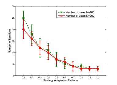
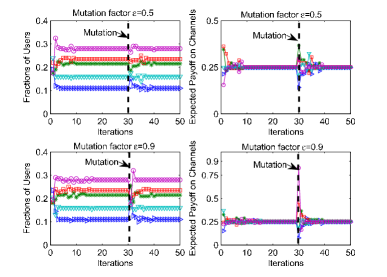
Figure 3: The iterations need for the convergence of the evolutionary spectrum accessing mechanism with different choices of strategy adaptation factor $\alpha$. The confidence interval is $95\%$.

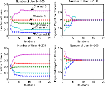
Figure 4: The fraction of users on each channel and the expected user payoff of accessing different channels with the number of users $N=100$ and $200$, respectively, and the number of backoff mini-slots $\lambda_{max}=100000$.

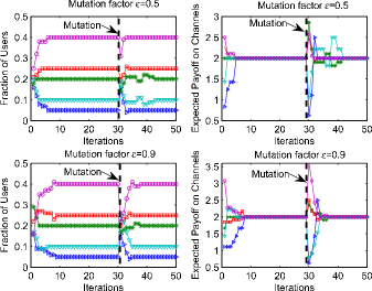
Figure 5: Stability of the evolutionary spectrum access mechanism. Fraction of users in total $N=200$ users who choose mutant channels randomly at time slot $30$ equal to $0.5$ and $0.9$, respectively, and the number of backoff mini-slots $\lambda_{max}=100000$.

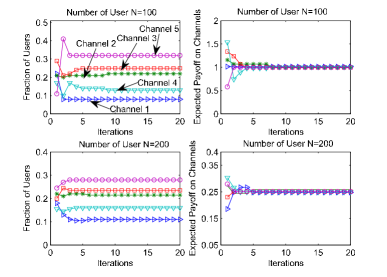
Figure 6: The fraction of users on each channel and the expected user payoff of accessing different channels with the number of users $N=100$ and $200$, respectively, and the number of backoff mini-slots $\lambda_{max}=20$.

Figure 7: Stability of the evolutionary spectrum access mechanism. Fraction of users in total $N=200$ users who choose mutant channels randomly at time slot $30$ equal to $0.5$ and $0.9$, respectively, and the number of backoff mini-slots $\lambda_{max}=20$.

VI-A Evolutionary Spectrum Access in Large User Population Case

We first study the evolutionary spectrum mechanism with complete network information in Section IV with a large user population. We found that the convergence speed of the evolutionary spectrum access mechanism increases as the strategy adaptation factor $\alpha$ increases (see Figure 3). We set the strategy adaptation factor $\alpha=0.5$ in the following simulations in order to better demonstrate the evolutionary dynamics. We implement the evolutionary spectrum access mechanism with the number of users $N=100$ and $200$, respectively, in both large and small $\lambda_{max}$ cases.

VI-A1 Large $\lambda_{max}$ Case

We first consider the case that the number of backoff mini-slots $\lambda_{max}=100000$, which is much larger that the number of users $N$ and thus collisions in channel contention rarely occur. This case can be approximated by the asymptotic case $\lambda_{max}=\infty$ in Section IV-C. The simulation results are shown in Figures 4 and 5. From these figures, we see that

• Fast convergence: the algorithm takes less than $20$ iterations to converge in all cases (see Figure 4).

• Convergence to ESS: in both $N=100$ and $200$ cases, the algorithm converges to the ESS $\boldsymbol{x}^{*}=\left(\frac{\theta_{1}B_{1}}{\sum_{i=1}^{M}\theta_{i}B_{i}},...,\frac{\theta_{M}B_{M}}{\sum_{i=1}^{M}\theta_{i}B_{i}}\right)$ (see Figure the left column of 4). At the ESS $\boldsymbol{x}^{*}$, each user achieves the same expected payoff $U_{n}(a_{n}^{*},\boldsymbol{x}^{*})=\frac{\sum_{i=1}^{M}\theta_{i}B_{i}}{N}$ (see the right column of Figure 4).

• Asymptotic stability: to investigate the stability of the evolutionary spectrum access mechanism, we let a fraction of users play the mutant strategies when the system is at the ESS $\boldsymbol{x}^{*}$. At time slot $t=30$, $\epsilon=0.5$ and $0.9$ fraction of users will randomly choose a new channel. The result is shown in Figure 5. We see that the algorithm is capable to recover the ESS $\boldsymbol{x}^{*}$ quickly after the mutation occurs. This demonstrates that the evolutionary spectrum access mechanism is robust to the perturbations in the network.

VI-A2 Small $\lambda_{max}$ Case

We now consider the case that the number of backoff mini-slots $\lambda_{max}=20$, which is smaller than the number of users $N$. In this case, severe collisions in channel contention may occur and hence lead to a reduction in data rates for all users. The results are shown in Figures 6 and 7. We see that a small $\lambda_{max}$ leads to a system performance loss (i.e., $\sum_{n=1}^{N}U_{n}(a_{n}(T),\boldsymbol{x}(T))<\sum_{m=1}^{M}\theta_{m}B_{m}$), due to severe collisions in channel contention. However, the evolutionary spectrum access mechanism still quickly converges to the ESS as given in (7) such that all users achieve the same expected throughput, and the asymptotic stable property also holds. This verifies the efficiency of the mechanism in the small $\lambda_{max}$ case.

VI-B Distributed Learning Mechanism in Large User Population Case

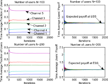
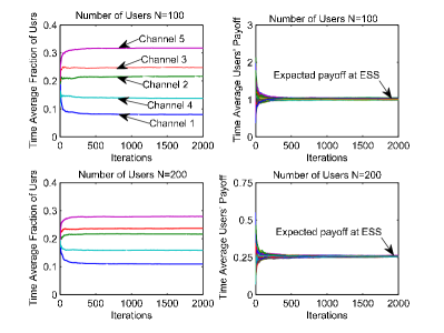
We next evaluate the learning mechanism for distributed spectrum access with a large user population. We implement the learning mechanism with the number of users $N=100$ and $N=200$, respectively, in both large and small $\lambda_{max}$ cases. We set the memory factor $\gamma=0.99$ and the length of a decision period $t_{\max}=100$ time slots, which provides a good estimation of the mean data rate. Figures 8 and 9 show the time average user distribution on the channels converges to the ESS, and the time average user’s payoff converges the expected payoff at the ESS. Note that users achieve this result without prior knowledge of the statistics of the channels, and the number of users utilizing each channel keeps changing in the learning scheme.

Figure 8: Learning mechanism for distributed spectrum access with the number of users $N=100$ and $200$, respectively, and the number of backoff mini-slots $\lambda_{max}=100000$.

Figure 9: Learning mechanism for distributed spectrum access with the number of users $N=100$ and $200$, respectively, and the number of backoff mini-slots $\lambda_{max}=20$.

VI-C Evolutionary Spectrum Access and Distributed Learning in Small User Population Case

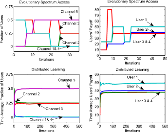
We then consider the case that the user population $N$ is small. We implement the proposed evolutionary spectrum access mechanism and distributed learning mechanism with the number of users $N=4$ and the number of backoff mini-slots $\lambda_{\max}=20$. The results are shown in Figure 10. We see that the evolutionary spectrum access mechanism converges to the equilibrium such that channel $5$ has $2$ users and both channel $1$ and $2$ have $1$ user. These $4$ users achieve the expected throughput equal to $50$, $40$, $38$ and $38$ Mbps, respectively, at the equilibrium. It is easy to check that any user unilaterally changes its channel selection at the equilibrium will lead to a loss in throughput, hence the equilibrium is a strict Nash equilibrium. According to [22], any strict Nash equilibrium is also an ESS and hence the convergent equilibrium is an ESS. For the distributed learning mechanism, we see that the mechanism also converges to the same equilibrium on the time average. This verifies that effectiveness of the proposed mechanisms in the small user population case.

Figure 10: Evolutionary spectrum access and Learning mechanism for distributed spectrum access with the number of users $N=4$, and the number of backoff mini-slots $\lambda_{max}=20$.

VI-D Performance Comparison

To benchmark the performance of the proposed mechanisms, we compare them with the following two algorithms:

• Centralized optimization: we solve the centralized optimization problem $\max_{\boldsymbol{x}}\sum_{n=1}^{N}U_{n}(a_{n},\boldsymbol{x})$, i.e., find the optimal population state $\boldsymbol{x}_{opt}$ that maximizes the system throughput.

• Distributed reinforcement learning: we also implement the distributed algorithm in [16] by generalizing the single-agent reinforcement learning to the multi-agent setting. More specifically, each user $n$ maintains a perception value $P_{m}^{n}(T)$ to describe the performance of channel $m$, and select the channel $m$ with the probability $f_{m,n}(T)=\frac{e^{\nu P_{m}^{n}(T)}}{\sum_{m^{\prime}=1}^{M}e^{\nu P_{m^{\prime}}^{n}(T)}}$ where $\nu$ is called the temperature. Once a payoff $U_{n}(T)$ is received, user $n$ updates the perception value as $P_{m}^{n}(T+1)=(1-\mu_{T})P_{m}^{n}(T)+\mu_{T}U_{n}(T)I_{\{a_{n}(T)=m\}}$ where $\mu_{T}$ is the smooth factor satisfying $\sum_{T=1}^{\infty}\mu_{T}=\infty$ and $\sum_{T=1}^{\infty}\mu_{T}^{2}<\infty$. As shown in [16], when $\nu$ is sufficiently large, the algorithm converges to a stationary point. We hence set $\mu_{T}=\frac{100}{T}$ and $\nu=10$ in the simulation, which guarantees the convergence and achieves a good system performance.

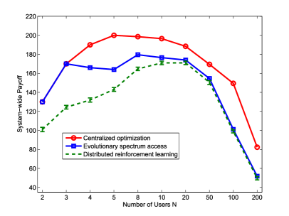
Since the proposed learning mechanism in this paper can converge to the same equilibrium as the evolutionary spectrum access mechanism, we only implement the evolutionary spectrum access mechanism in this experiment. The results are shown in Figure 11. Since the global optimum by centralized optimization and the ESS by evolutionary spectrum access are deterministic, only the confidence interval of the distributed reinforcement learning is shown here. We see that the evolutionary spectrum access mechanism achieves up to $35\%$ performance improvement over the distributed reinforcement learning algorithm. Compared with the centralized optimization approach, the performance loss of the evolutionary spectrum access mechanism is at most $38\%$. When the number of users $N$ is small (e.g., $N\leq 50$), the performance loss can be further reduced to less than $25\%$. Note that the solution by the centralized optimization is not incentive compatible, since it is not a Nash equilibrium and user can improve its payoff by changing its channel selection unilaterally. While the evolutionary spectrum access mechanism achieves an ESS, which is also a (strict) Nash equilibrium and evolutionarily stable. Interestingly, the curve of the evolutionary spectrum access mechanism in Figure 11 achieves a local minimum when the number of users $N=5$. This can be interpreted by the property of the Nash equilibrium. When the number of users $N=4$, these four users will utilize the three channels with high data rate (i.e., Channel $2$, $3$, and $5$ in the simulation). When the number of users $N=5$, the same three channels are utilized at the Nash equilibrium. In this case, there will be a system performance loss due to severer channel contention. However, no user at the equilibrium is willing to switch to another vacant channel, since the remaining vacant channels have low data rates and such a switch will incurs a loss to the user. When the number of users $N=8$, all given channels are utilized at the Nash equilibrium, and this improves the system performance.

Figure 11: Comparison of the evolutionary spectrum access mechanism with the distributed reinforcement learning and centralized optimization. The confidence interval is $95\%$.

Figure 12: Two states Markovian channel model

VI-E Distributed Learning Mechanism In Markovian Channel Environment

For the ease of exposition, we have considered the i.i.d. channel model as far. We now consider the proposed mechanisms in the Markovian channel environment. Since in the evolutionary spectrum access mechanism each user has the complete information aprior (including the stationary distribution that a channel is idle), the Markovian setting will not affect the evolutionary spectrum access mechanism. We hence focus on evaluating the learning mechanism.

We consider a network of $N=100$ users and $M=10$ channels. The states of channels change according to independent Markovian processes (see Figure 12). We denote the channel state probability vector of channel $m$ at time slot $t$ as $\boldsymbol{p}_{m}(t)\triangleq(Pr\{S_{m}(t)=0,Pr\{S_{m}(t)=1\}\}),$ which follows a two state Markov chain as $\boldsymbol{p}_{m}(t)=\boldsymbol{p}_{m}(t-1)\Gamma,\forall t\geq 1$, with the transition matrix

$$\Gamma=\left[\begin{array}[]{cc}1-p&p\\ q&1-q\end{array}\right].$$

For the simulation, we set $p=q=\epsilon,$ where $\epsilon$ is called the dynamic factor. A larger $\epsilon$ means that the channel state changes faster over time. The mean data rates $B_{m}$ of $10$ channels are $10,40,50,20,80,60,15,25,30,$ and $70$ Mbps, respectively.

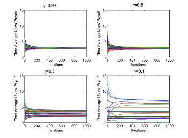
We first set the dynamic factor $\epsilon=0.3$, and study the learning mechanism with the different memory weights $\gamma=0.99,0.8,0.5,$ and $0.1$, respectively. The results are shown in Figure 13. We see that a large enough memory weight (e.g., $\gamma\geq 0.8$) is needed to guarantee that the mechanism converges to the ESS equilibrium. When the memory weight is large, the noise of the local estimation by each user can be averaged out in the long run, and hence each user can achieve an accurate estimation of the environment. When the memory weight is small, the most recent estimations will have a great impact on the learning. This means that the learning mechanism will over-exploit the current best channels, and get stuck in a local optimum.

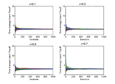
We next set the memory weight $\gamma=0.99$, and investigate the learning mechanism in the Markovian channel environments with different dynamic factors $\epsilon=0.1,0.3,0.5,$ and $0.7$, respectively. The results are shown in Figure 14. We see that the learning mechanism can converge to the ESS in all cases. This demonstrates that the learning mechanism is robust to the dynamic channel state changing.

Figure 13: Distributed learning mechanism with different memory weights $\gamma$

Figure 14: Distributed learning mechanism with the memory weight $\gamma=0.99$ in the Markovian channel environment with different dynamic factors $\epsilon$

VII Conclusion

In this paper, we study the problem of distributed spectrum access of multiple time-varying heterogeneous licensed channels, and propose an evolutionary spectrum access mechanism based on evolutionary game theory. We show that the equilibrium of the mechanism is an evolutionarily stable strategy and is globally stable. We further propose a learning mechanism, which requires no information exchange among the users. We show that the learning mechanism converges to the evolutionarily stable strategy on the time average. Numerical results show that the proposed mechanisms can achieve efficient and stable spectrum sharing among the users.

One possible direction of extending this result is to consider heterogeneous users, i.e. each user may achieve different mean data rates on the same channel. Another interesting direction is to take the spatial reuse effect into account. How to design an efficient evolutionarily stable spectrum access mechanism with spatial reuse will be challenging.

VIII Appendix

VIII-A Proof of Theorem 1

Given a population state $\boldsymbol{x}(t)=(x_{1}(t),...,x_{M}(t)),$ we divide the set of channels $\mathcal{M}$ into the following three complete and mutually exclusive subsets: $\mathcal{M}_{1}=\{m\in\mathcal{M}|\theta_{m}B_{m}g(Nx_{m}(t))<U(\boldsymbol{x}(t))\}$, $\mathcal{M}_{2}=\{m\in\mathcal{M}|\theta_{m}B_{m}g(Nx_{m}(t))=U(\boldsymbol{x}(t))\}$, and $\mathcal{M}_{3}=\{m\in\mathcal{M}|\theta_{m}B_{m}g(Nx_{m}(t))>U(\boldsymbol{x}(t))\}$.

For a channel $m\in\mathcal{M}_{1}$, each user $n$ on this channel achieves an expected payoff less than the system average payoff, i.e., $U_{n}(m,\boldsymbol{x}(t))=\theta_{m}B_{m}g(Nx_{m}(t))<U(\boldsymbol{x}(t))$. According to the mechanism, each user has a probability of $\frac{\alpha}{x_{m}(t)}\left(1-\frac{U_{n}(m,\boldsymbol{x}(t))}{U(\boldsymbol{x}(t))}\right)$ to move out of the channel $m$. Since $\theta_{m}B_{m}g(Nx_{m}(t))<U(\boldsymbol{x}(t))$, it follows that $p_{m}=0$ and hence no other users will move into this channel. Thus, the dynamics are given as

$$\dot{x}_{m}(t) = -\frac{\alpha}{x_{m}(t)}\left(1-\frac{U_{n}(m,\boldsymbol{x}(t))}{U(\boldsymbol{x}(t))}\right)x_{m}(t)$$

$$= \alpha\left(\frac{U_{n}(m,\boldsymbol{x}(t))}{U(\boldsymbol{x}(t))}-1\right),\forall m\in\mathcal{M}_{2}.$$

For a channel $m\in\mathcal{M}_{2}$, we have $U_{n}(m,\boldsymbol{x}(t))=U(\boldsymbol{x}(t))$ and $p_{m}=0$. Thus, $\dot{x}_{m}(t)=0$, which satisfies the conclusion.

For a channel $m\in\mathcal{M}_{3}$, each user $n$ on this channel achieves an expected payoff higher than the system average payoff, i.e., $U_{n}(m,\boldsymbol{x}(t))=\theta_{m}B_{m}g(Nx_{m}(t))>U(\boldsymbol{x}(t))$. According to the mechanism, no users will move out of the channel $m$. Since $p_{m}>0$, there will be some other users from the channel $m^{\prime}\in\mathcal{M}_{1}$ moving into this channel. Let $\omega$ be the fraction of population that carries out the movement. We have

$$\omega= \sum_{m^{\prime}\in\mathcal{M}_{1}}\left(x_{m^{\prime}}(t)-x_{m^{\prime}}(t+1)\right)$$

$$= \sum_{m^{\prime}\in\mathcal{M}_{1}}\alpha\left(1-\frac{U_{n}(m^{\prime},\boldsymbol{x}(t))}{U(\boldsymbol{x}(t))}\right)$$

$$= \sum_{m^{\prime}\in\mathcal{M}_{1}}\frac{\alpha}{U(\boldsymbol{x}(t))}\left(U(\boldsymbol{x}(t))-U_{n}(m^{\prime},\boldsymbol{x}(t))\right)$$

$$= \frac{\alpha}{U(\boldsymbol{x}(t))}\sum_{m^{\prime}\in\mathcal{M}_{1}}\left(U(\boldsymbol{x}(t))-\theta_{m^{\prime}}B_{m^{\prime}}g(Nx_{m^{\prime}}(t))\right).$$

Since $\theta_{m^{\prime}}B_{m^{\prime}}g(Nx_{m^{\prime}}(t))=U(\boldsymbol{x}(t))$ for each channel $m^{\prime}\in\mathcal{M}_{2}$, and $\sum_{m^{\prime}\in\mathcal{M}}\left(U(\boldsymbol{x}(t))-\theta_{m^{\prime}}B_{m^{\prime}}g(Nx_{m^{\prime}}(t))\right)=0$, we then obtaion

$$\sum_{m^{\prime}\in\mathcal{M}_{1}}\left(U(\boldsymbol{x}(t))-\theta_{m^{\prime}}B_{m^{\prime}}g(Nx_{m^{\prime}}(t))\right)$$

$$= \sum_{m^{\prime}\in\mathcal{M}_{3}}\left(\theta_{m^{\prime}}B_{m^{\prime}}g(Nx_{m^{\prime}}(t))-U(\boldsymbol{x}(t))\right).$$

Then, the fraction of the population moving into a channel $m\in\mathcal{M}_{3}$ thus is

$$\dot{x}_{m}(t)=p_{m}\omega$$

$$= \frac{\left(\theta_{m}B_{m}g(Nx_{m}(t))-U(\boldsymbol{x}(t))\right)}{\sum_{m^{\prime}\in\mathcal{M}_{3}}\left(\theta_{m^{\prime}}B_{m^{\prime}}g(Nx_{m^{\prime}}(t))-U(\boldsymbol{x}(t))\right)}$$

$$\times\frac{\alpha}{U(\boldsymbol{x}(t))}\sum_{m^{\prime}\in\mathcal{M}_{3}}\left(\theta_{m^{\prime}}B_{m^{\prime}}g(Nx_{m^{\prime}}(t))-U(\boldsymbol{x}(t))\right)$$

$$= \alpha\left(\frac{U_{n}(m,\boldsymbol{x}(t))}{U(\boldsymbol{x}(t))}-1\right),\forall m\in\mathcal{M}_{3}.$$

This completes the proof. ∎

VIII-B Proof of Theorem 2

First, it is easy to check that when $x_{m}(t)=x_{m}^{*}=\frac{\theta_{m}B_{m}}{\sum_{i=1}^{M}\theta_{i}B_{i}}$, we have $\dot{x}_{m}(t)=0$ in the evolutionary dynamics (6). Thus, $\boldsymbol{x}(t)$ is the equilibrium of the evolutionary dynamics.

We then apply Lyapunov’s second method [26] to prove that the equilibrium $\boldsymbol{x}^{*}$ is globally asymptotic stable. We use the following Lyapunov function $V(\boldsymbol{x}(t))=-\sum_{m=1}^{M}x_{m}^{*}\ln\frac{x_{m}(t)}{x_{m}^{*}}$. By Jensen’s inequality, we first have for any $\boldsymbol{x}(t)\neq\boldsymbol{x}^{*}$

$$V(\boldsymbol{x}(t)) > -\ln\left(\sum_{m=1}^{M}x_{m}^{*}\frac{x_{m}(t)}{x_{m}^{*}}\right)$$

$$= -\ln\left(\sum_{m=1}^{M}x_{m}(t)\right)=0.$$

Thus, we obtain that $V(\boldsymbol{x}^{*})=0$ and $V(\boldsymbol{x}(t))>0$ for any $\boldsymbol{x}(t)\neq\boldsymbol{x}^{*}$.

We then consider the time derivative of $V(\boldsymbol{x}(t))$ as

$$\frac{dV(\boldsymbol{x}(t))}{dt}$$

$$= -\sum_{m=1}^{M}\frac{\partial V(\boldsymbol{x}(t))}{\partial x_{m}(t)}\dot{x}_{m}(t)=-\sum_{m=1}^{M}\frac{x_{m}^{*}}{x_{m}(t)}\dot{x}_{m}(t)$$

$$= -\frac{\alpha}{\frac{1}{M}\sum_{i=1}^{M}\frac{\theta_{i}B_{i}}{x_{i}(t)}}\sum_{m=1}^{M}\frac{x_{m}^{*}}{x_{m}(t)}\left(\frac{\theta_{m}B_{m}}{x_{m}(t)}-\frac{1}{M}\sum_{i=1}^{M}\frac{\theta_{i}B_{i}}{x_{i}(t)}\right)$$

$$= -\frac{\alpha}{M\left(\sum_{j=1}^{M}\theta_{j}B_{j}\right)\left(\frac{1}{M}\sum_{i=1}^{M}\frac{\theta_{i}B_{i}}{x_{i}(t)}\right)}$$

$$\times\left(M\sum_{m=1}^{M}\left(\frac{\theta_{m}B_{m}}{x_{m}(t)}\right)^{2}-\sum_{m=1}^{M}\sum_{i=1}^{M}\frac{\theta_{m}B_{m}}{x_{m}(t)}\frac{\theta_{i}B_{i}}{x_{i}(t)}\right)$$

$$= -\frac{\alpha}{\left(\sum_{j=1}^{M}\theta_{j}B_{j}\right)\left(\sum_{i=1}^{M}\frac{\theta_{i}B_{i}}{x_{i}(t)}\right)}$$

$$\times\sum_{m=1}^{M}\sum_{i=1}^{M}\left(\frac{\theta_{m}B_{m}}{x_{m}(t)}-\frac{\theta_{i}B_{i}}{x_{i}(t)}\right)^{2}.$$

Thus, we must have that $\frac{dV(\boldsymbol{x}^{*})}{dt}=0$ and $\frac{dV(\boldsymbol{x}(t))}{dt}<0$ for any $\boldsymbol{x}(t)\neq\boldsymbol{x}^{*},$ which completes the proof. ∎

According to [22], any strict Nash equilibrium is also an ESS and hence the equilibrium $\boldsymbol{x}^{*}$ is an ESS. ∎

VIII-C Proof of Theorem 4

According to Lyapunov’s second method [26], we prove the global asymptotic stability by using the following Lyapunov function $V(\boldsymbol{x}(t))=L^{*}-L(\boldsymbol{x}(t))$. Since $L^{*}$ is the unique global maximum of $L(\boldsymbol{x}(t))$ achieved at $\boldsymbol{x}^{*}$, we thus have

$$V(\boldsymbol{x}(t)) > 0,\forall\boldsymbol{x}(t)\neq\boldsymbol{x}^{*},$$

$$V(\boldsymbol{x}^{*}) = 0.$$

Then differentiating $V(\boldsymbol{x}(t))$ with respective to time $t$, we have

$$\dot{V}(\boldsymbol{x}(t))$$

$$= -\sum_{m=1}^{M}B_{m}g(Nx_{m})\dot{x}_{m}(t)$$

$$= -\sum_{m=1}^{M}U_{n}(m,\boldsymbol{x}(t))\dot{x}_{m}(t)$$

$$= -\sum_{m=1}^{M}U_{n}(m,\boldsymbol{x}(t))\frac{\alpha}{U(\boldsymbol{x}(t))}\left(U_{n}(m,\boldsymbol{x}(t))-U(\boldsymbol{x}(t))\right)$$

$$= -\frac{\alpha}{MU(\boldsymbol{x}(t))}\left(M\sum_{m=1}^{M}\left(U_{n}(m,\boldsymbol{x}(t))\right)^{2}\right.$$

$$\left.-\sum_{m=1}^{M}U_{n}(m,\boldsymbol{x}(t))\sum_{m^{\prime}=1}^{M}U_{n}(m^{\prime},\boldsymbol{x}(t))\right)$$

$$= -\frac{\alpha}{MU(\boldsymbol{x}(t))}\sum_{m=1}^{M}\sum_{m^{\prime}=1}^{M}\left(U_{n}(m,\boldsymbol{x}(t))-U_{n}(m^{\prime},\boldsymbol{x}(t))\right)^{2}$$

Thus, we obtain that

$$\dot{V}(\boldsymbol{x}(t)) < 0,\forall\boldsymbol{x}(t)\neq\boldsymbol{x}^{*},$$

$$\dot{V}(\boldsymbol{x}^{*}) = 0,$$

which completes the proof. ∎

VIII-D Proof of Theorem 3

We first show that the solution in (7) is an equilibrium for the evolution dynamics in (4). Since $U_{n}(m,\boldsymbol{x}^{*})=U_{n}(m^{\prime},\boldsymbol{x}^{*})$ for any $m,m^{\prime}\in\mathcal{M}$, it follows that $U(\boldsymbol{x}^{*})=\frac{1}{M}\sum_{i=1}^{M}U_{n}(i,\boldsymbol{x}^{*})=U_{n}(m,\boldsymbol{x}^{*})$ for any $m\in\mathcal{M}.$ Hence $\dot{x}_{m}=\alpha(\frac{U_{n}(m,\boldsymbol{x}^{*})}{U(\boldsymbol{x}^{*})}-1)=0$, which is an equilibrium for the evolution dynamics in (4).

We next show that the equilibrium $\boldsymbol{x}^{*}$ is a strict Nash equilibrium. The expected payoff of a user $n\in\mathcal{N}$ at the equilibrium population state $\boldsymbol{x}^{*}$ is given by $U_{n}(a_{n}^{*},\boldsymbol{x}^{*})=\theta_{a_{n}^{*}}B_{a_{n}^{*}}g(Nx_{a_{n}^{*}}^{*}),$ where $a_{n}^{*}$ is the channel chosen by user $n$ in the population state $\boldsymbol{x}^{*}$. Now suppose that user $n$ makes an unilateral deviation to another channel $a_{n}\neq a_{n}^{*}$, and the population state becomes $\boldsymbol{x}^{\prime}=(x_{1}^{*},...,x_{a_{n}^{*}-1}^{*},x_{a_{n}^{*}}^{*}-\frac{1}{N},x_{a_{n}^{*}+1}^{*},...,x_{a_{n}-1}^{*},x_{a_{n}}^{*}+\frac{1}{N},x_{a_{n}+1}^{*},...,x_{N}^{*})$. Then its expected payoff becomes $U_{n}(a_{n},\boldsymbol{x}^{\prime})=\theta_{a_{n}}B_{a_{n}}g(Nx_{a_{n}}^{*}+1)<\theta_{a_{n}}B_{a_{n}}g(Nx_{a_{n}}^{*}).$ For the equilibrium $\boldsymbol{x}^{*}$, we have $\theta_{a_{n}^{*}}B_{a_{n}^{*}}g(Nx_{a_{n}^{*}}^{*})=\theta_{a_{n}}B_{a_{n}}g(Nx_{a_{n}}^{*}).$ It follows that $U_{n}(a_{n}^{*},\boldsymbol{x}^{*})>U_{n}(a_{n},\boldsymbol{x}^{\prime}),\forall a_{n}\neq a_{n}^{*},n\in\mathcal{N}$, which is a strict Nash equilibrium.

VIII-E Proof of Theorem 5

The key idea of the proof is to first obtain the discrete time dynamics of the learning mechanism, and then derive the corresponding mean continuous time dynamics.

For simplicity, we first define that

$$A_{m,n}(T)=\sum_{\tau=0}^{T-1}\gamma^{T-\tau-1}Z_{m,n}(\tau)$$

and

$$C_{n}(T)=\frac{\sum_{t=1}^{t_{\max}}b_{i}(t)I_{\{a_{n}(t,T)=a_{n}(T)\}}}{t_{\max}},$$

where $I_{\{a_{n}(t,T)=a_{n}(T)\}}$ indicates whether user $n$ successfully grabs the chosen channel $a_{n}(T)$, and hence $C_{n}(T)$ denotes the average throughput it received at period $T$. According to (11) and (12), we have

$$A_{m,n}(T+1)=Z_{m,n}(T)+\gamma\sum_{\tau=0}^{T-1}\gamma^{T-\tau-1}Z_{m,n}(\tau)$$

$$= (1-\gamma)C_{n}(T)I_{\{a_{n}(T)=m\}}+(1-\gamma)\sum_{\tau=0}^{T-1}\gamma^{T-\tau-1}Z_{m,n}(\tau)$$

$$+\gamma\sum_{\tau=0}^{T-1}\gamma^{T-\tau-1}Z_{m,n}(\tau)$$

$$= (1-\gamma)C_{n}(T)I_{\{a_{n}(T)=m\}}+\sum_{\tau=0}^{T-1}\gamma^{T-\tau-1}Z_{m,n}(\tau)$$

$$= (1-\gamma)C_{n}(T)I_{\{a_{n}(T)=m\}}+A_{m,n}(T),$$

where $I_{\{a_{n}(T)=m\}}$ indicates whether user $n$ chooses channel $m$ in period $T$. Then the mixed strategy update in (10) becomes

$$f_{m,n}(T+1)=\frac{A_{m,n}(T+1)}{\sum_{i=1}^{M}A_{i,n}(T+1)}$$

$$= \frac{A_{m,n}(T)+(1-\gamma)C_{n}(T)I_{\{a_{n}(T)=m\}}}{\sum_{i=1}^{M}A_{i,n}(T)+(1-\gamma)C_{n}(T)},$$

For the chosen channel $j$ (i.e., $I_{\{a_{n}(T)=j\}}=1$), we further have

$$f_{j,n}(T+1)=\frac{A_{j,n}(T)}{\sum_{i=1}^{M}A_{i,n}(T)+(1-\gamma)C_{n}(T)}$$ (15)

$$+\frac{(1-\gamma)C_{n}(T)}{\sum_{i=1}^{M}A_{i,n}(T)+(1-\gamma)C_{n}(T)}$$

$$= \frac{A_{j,n}(T)}{\sum_{i=1}^{M}A_{i,n}(T)}\frac{\sum_{i=1}^{M}A_{i,n}(T)}{\sum_{i=1}^{M}A_{i,n}(T)+(1-\gamma)C_{n}(T)}$$

$$+\frac{(1-\gamma)C_{n}(T)}{\sum_{i=1}^{M}A_{i,n}(T)+(1-\gamma)C_{n}(T)}$$

$$= f_{j,n}(T)\left(1-\frac{(1-\gamma)C_{n}(T)}{\sum_{i=1}^{M}A_{i,n}(T)+(1-\gamma)C_{n}(T)}\right)$$

$$+\frac{(1-\gamma)C_{n}(T)}{\sum_{i=1}^{M}A_{i,n}(T)+(1-\gamma)C_{n}(T)}.$$ (16)

Let $\beta(T)=\frac{(1-\gamma)}{\sum_{i=1}^{M}A_{i,n}(T)+(1-\gamma)C_{n}(T)}$, and (16) can be expresses as

$$f_{j,n}(T+1)=f_{j,n}(T)(1-\beta(T)C_{n}(T))+\beta(T)C_{n}(T).$$ (17)

Similarly, for the unchosen channel $j^{\prime}$(i.e., $I_{\{a_{n}(T)=j^{\prime}\}}=0$), we have

$$f_{j^{\prime},n}(T+1)=f_{j^{\prime},n}(T)(1-\beta(T)C_{n}(T)).$$ (18)

According to (17) and (18), we thus obtain the discrete time learning dynamics as

$$f_{m,n}(T+1)-f_{m,n}(T)=\beta(T)C_{n}(T)(I_{\{a_{n}(T)=m\}}-f_{m,n}(T)).$$ (19)

Since $\beta(T)\rightarrow 0$ as $\gamma\rightarrow 1$, by the theory of stochastic approximation (Theorem 3.2) in [25], the limiting behavior of the stochastic difference equations in (19) is the same as its mean continuous time dynamics by taking the expectation on RHS of (19) with respective to $\boldsymbol{f}(T)$, i.e.,

$$\dot{f}_{m,n}(T)=E[C_{n}(T)(I_{\{a_{n}(T)=m\}}-f_{m,n}(T))|\boldsymbol{f}(T)]$$

$$= (1-f_{m,n}(T))E[C_{n}(T)|a_{n}(t)=m,\boldsymbol{f}(T)]f_{m,n}(T)$$

$$-f_{m,n}(T)\sum_{i\neq m}E[C_{n}(T)|a_{n}(t)=i,\boldsymbol{f}(T)]f_{i,n}(T).$$ (20)

Since $C_{n}(T)$ is the sample averaging estimation of the expected throughput of the chosen channel, by the central limit theorem, we have $E[C_{n}(T)|a_{n}(t)=m,\boldsymbol{f}(T)]=E[U_{n}(a_{n}(t)=m,\boldsymbol{x}(T))|\boldsymbol{f}(T)]=Q_{m,n}(\boldsymbol{f}(T))$. Then the mean dynamics in (20) can be written as

$$\dot{f}_{m,n}(T) =Q_{m,n}(\boldsymbol{f}(T))(1-f_{m,n}(T))f_{m,n}(T)$$

$$-f_{m,n}(T)\sum_{i\neq m}Q_{i,n}(\boldsymbol{f}(T))f_{i,n}(T)$$

$$= f_{m,n}(T)\left(Q_{m,n}(\boldsymbol{f}(T))-\sum_{i=1}^{M}Q_{i,n}(\boldsymbol{f}(T))f_{i,n}(T)\right),$$

which completes the proof. ∎

VIII-F Proof of Theorem 6

We first denote the following function

$$\Phi(\boldsymbol{f}(T))=E[\sum_{i=1}^{M}\int_{-\infty}^{x_{i}(T)}\theta_{i}B_{i}g(Nz)dz|\boldsymbol{f}(T)],$$

and

$$\Phi_{m,n}(\boldsymbol{f}(T))=E[\sum_{i=1}^{M}\int_{-\infty}^{x_{i}(T)}\theta_{i}B_{i}g(Nz)dz|a_{n}(T)=m,\boldsymbol{f}(T)].$$

Obviously, we have

$$\Phi(\boldsymbol{f}(T))=\sum_{m=1}^{M}\Phi_{m,n}(\boldsymbol{f}(T))f_{m,n}(T).$$

We further denote $\boldsymbol{x}_{-n}(T)\triangleq\left(x_{m}^{-n}(T),m\in\mathcal{M}\right)$ as the population state of all other users without user $n$. By considering the user distributions on the chosen channel $m$ by user $n$ and the other channels, we then have

$$\Phi_{m,n}(\boldsymbol{f}(T))$$

$$= E[\sum_{i=1}^{M}\int_{-\infty}^{x_{i}(T)}\theta_{i}B_{i}g(Nz)dz|a_{n}(T)=m,\boldsymbol{f}(T)]$$

$$= \sum_{\boldsymbol{x}_{-n}(T)}E[\sum_{i\neq m}\int_{-\infty}^{x_{i}^{-n}(T)}\theta_{i}B_{i}g(Nz)dz$$

$$+\int_{-\infty}^{x_{m}^{-n}(T)+\frac{1}{N}}\theta_{m}B_{m}g(Nz)dz|a_{n}(T)=m,\boldsymbol{x}_{-n}(T)]$$

$$\times Pr\{\boldsymbol{x}_{-n}(T)|\boldsymbol{f}(T)\}$$

$$= \sum_{\boldsymbol{x}_{-n}(T)}\left(\sum_{i\neq m}\int_{-\infty}^{x_{i}^{-n}(T)}\theta_{i}B_{i}g(Nz)dz\right.$$

$$\left.+\int_{-\infty}^{x_{m}^{-n}(T)+\frac{1}{N}}\theta_{m}B_{m}g(Nz)dz\right)Pr\{\boldsymbol{x}_{-n}(T)|\boldsymbol{f}(T)\}.$$ (21)

Similarly, we can obtain

$$\Phi_{m^{\prime},n}(\boldsymbol{f}(T))=\sum_{\boldsymbol{x}_{-n}(T)}\left(\sum_{i\neq m^{\prime}}\int_{-\infty}^{x_{i}^{-n}(T)}\theta_{i}B_{i}g(Nz)dz\right.$$

$$\left.+\int_{-\infty}^{x_{m^{\prime}}^{-n}(T)+\frac{1}{N}}\theta_{m^{\prime}}B_{m^{\prime}}g(Nz)dz\right)Pr\{\boldsymbol{x}_{-n}(T)|\boldsymbol{f}(T)\}.$$ (22)

It follows that

$$\Phi_{m,n}(\boldsymbol{f}(T))-\Phi_{m^{\prime},n}(\boldsymbol{f}(T))$$

$$= \sum_{\boldsymbol{x}_{-n}(T)}\left(\sum_{i\neq m}\int_{-\infty}^{x_{i}^{-n}(T)}\theta_{i}B_{i}g(Nz)dz\right.$$

$$\left.+\int_{-\infty}^{x_{m}^{-n}(T)+\frac{1}{N}}\theta_{m}B_{m}g(Nz)dz\right)Pr\{\boldsymbol{x}_{-n}(T)|\boldsymbol{f}(T)\}$$

$$-\sum_{\boldsymbol{x}_{-n}(T)}\left(\sum_{i\neq m^{\prime}}\int_{-\infty}^{x_{i}^{-n}(T)}\theta_{i}B_{i}g(Nz)dz\right.$$

$$\left.+\int_{-\infty}^{x_{m^{\prime}}^{-n}(T)+\frac{1}{N}}\theta_{m^{\prime}}B_{m^{\prime}}g(Nz)dz\right)Pr\{\boldsymbol{x}_{-n}(T)|\boldsymbol{f}(T)\}$$

$$= \sum_{\boldsymbol{x}_{-n}(T)}\left(\int_{-\infty}^{x_{m}^{-n}(T)+\frac{1}{N}}\theta_{m}B_{m}g(Nz)dz\right.$$

$$\left.-\int_{-\infty}^{x_{m}^{-n}(T)}\theta_{m}B_{m}g(Nz)\right)Pr\{\boldsymbol{x}_{-n}(T)|\boldsymbol{f}(T)\}$$

$$-\sum_{\boldsymbol{x}_{-n}(T)}\left(\int_{-\infty}^{x_{m^{\prime}}^{-n}(T)+\frac{1}{N}}\theta_{m^{\prime}}B_{m^{\prime}}g(Nz)dz\right.$$

$$\left.-\int_{-\infty}^{x_{m^{\prime}}^{-n}(T)}\theta_{m^{\prime}}B_{m^{\prime}}g(Nz)\right)Pr\{\boldsymbol{x}_{-n}(T)|\boldsymbol{f}(T)\}.$$ (23)

Since $N$ is large, we obtain that for $i\in\{m,m^{\prime}\}$

$$\int_{-\infty}^{x_{i}^{-n}(T)+\frac{1}{N}}\theta_{i}B_{i}g(Nz)dz-\int_{-\infty}^{x_{i}^{-n}(T)}\theta_{i}B_{i}g(Nz)$$

$$= \int_{x_{i}^{-n}(T)}^{x_{i}^{-n}(T)+\frac{1}{N}}\theta_{i}B_{i}g(Nz)dz=\int_{Nx_{i}^{-n}(T)}^{Nx_{i}^{-n}(T)+1}\theta_{i}B_{i}g(z)dz$$

$$\approx \theta_{i}B_{i}g(Nx_{i}^{-n}(T)+1).$$ (24)

According to (23) and (24), we have

$$\Phi_{m,n}(\boldsymbol{f}(T))-\Phi_{m^{\prime},n}(\boldsymbol{f}(T))$$

$$= \sum_{\boldsymbol{x}_{-n}(T)}\left(\theta_{m}B_{m}g(Nx_{m}^{-n}(T)+1)\right.$$

$$-\left.\theta_{m^{\prime}}B_{m^{\prime}}g(Nx_{m^{\prime}}^{-n}(T)+1)\right)Pr\{\boldsymbol{x}_{-n}(T)|\boldsymbol{f}(T)\}$$

$$= E[U_{n}(a_{n}=m,\boldsymbol{x}(t))|\boldsymbol{f}(T)]-E[U_{n}(a_{n}=m^{\prime},\boldsymbol{x}(t))|\boldsymbol{f}(T)]$$

$$= Q_{m,n}(\boldsymbol{f}(T))-Q_{m^{\prime},n}(\boldsymbol{f}(T)).$$ (25)

We then consider the variation of $\Phi(\boldsymbol{f}(T))$ along the trajectories of learning dynamics in (13), i.e., differentiating $\Phi(\boldsymbol{f}(T))$ with respective to time $T$,

$$\frac{d\Phi(\boldsymbol{f}(T))}{dT}=\sum_{m=1}^{M}\frac{d\Phi(\boldsymbol{f}(T))}{df_{m,n}(T)}\frac{df_{m,n}(T)}{dT}$$

$$= \sum_{m=1}^{M}\Phi_{m,n}(\boldsymbol{f}(T))f_{m,n}(T)$$

$$\times\left(Q_{m,n}(\boldsymbol{f}(T))-\sum_{i=1}^{M}f_{i,n}(T)Q_{i,n}(\boldsymbol{f}(T))\right)$$

$$= \frac{1}{2}\sum_{m=1}^{M}\sum_{i=1}^{M}f_{m,n}(T)f_{i,n}(T)$$

$$\times\left(Q_{m,n}(\boldsymbol{f}(T))-Q_{i,n}(\boldsymbol{f}(T))\right)\left(\Phi_{m,n}(\boldsymbol{f}(T))-\Phi_{i,n}(\boldsymbol{f}(T))\right)$$

$$= \frac{1}{2}\sum_{i=1}^{M}\sum_{j=1}^{M}f_{i,n}(T)f_{j,n}(T)\left(Q_{i,n}(\boldsymbol{f}(T))-Q_{j,n}(\boldsymbol{f}(T))\right)^{2}$$

$$\geq 0.$$ (26)

Hence $\Phi(\boldsymbol{f}(T))$ is non-decreasing along the trajectories of the ODE (13). According to Theorem 2.7 in [26], the learning mechanism asymptotically converges to a limit point $\boldsymbol{f}^{*}$ such that

$$\frac{d\Phi(\boldsymbol{f}^{*})}{dT}=0,$$ (27)

i.e., for any $m,i\in\mathcal{M},n\in\mathcal{N}$

$$f_{m,n}^{*}f_{i,n}^{*}\left(Q_{m,n}(\boldsymbol{f}^{*})-Q_{i,n}(\boldsymbol{f}^{*})\right)=0.$$ (28)

According to the mixed strategy update in (10), we know that $f_{m,n}(T)>0$ for any $m\in\mathcal{M}$. Thus, from (28), we must have $Q_{m,n}(\boldsymbol{f}^{*})=Q_{i,n}(\boldsymbol{f}^{*})$. ∎

References

• [1] FCC, “Report of the spectrum efficiency group,” in Spectrum Policy Task Force, 2002.
• [2] I. Akyildiz, W. Lee, M. Vuran, and S. Mohanty, “Next generation/dynamic spectrum access/cognitive radio wireless networks: a survey,” Computer Networks, vol. 50, no. 13, pp. 2127–2159, 2006.
• [3] X. Chen and J. Huang, “Spatial spectrum access game: Nash equilibria and distributed learning,” in ACM International Symposium on Mobile Ad Hoc Networking and Computing (MobiHoc), 2012.
• [4] Z. Ji and K. J. R. Liu, “Dynamic spectrum sharing: A game theoretical overview,” IEEE Communications Magazine, vol. 45, pp. 88–94, 2007.
• [5] M. Liu and Y. Wu, “Spectrum sharing as congestion games,” in Annual Allerton Conference on Communication, Control, and Computing, 2008.
• [6] J. Elias, F. Martignon, A. Capone, and E. Altman, “Competitive interference-aware spectrum access in cognitive radio networks,” in 2010 Proceedings of the 8th International Symposium on Modeling and Optimization in Mobile, Ad Hoc and Wireless Networks (WiOpt), 2010.
• [7] N. Nie and Comniciu, “Adaptive channel allocation spectrum etiquette for cognitive radio networks,” in IEEE Symposium on New Frontiers in Dynamic Spectrum Access Networks (DySPAN), 2005.
• [8] L. M. Law, J. Huang, M. Liu, and S. Y. R. Li, “Price of anarchy of cognitive mac games,” in IEEE Global Communications Conference, 2009.
• [9] X. Chen and J. Huang, “Imitative spectrum access,” in International Symposium on Modeling and Optimization in Mobile, Ad Hoc and Wireless Networks (WiOpt),, 2012.
• [10] Z. Han, C. Pandana, and K. J. R. Liu, “Distributive opportunistic spectrum access for cognitive radio using correlated equilibrium and no-regret learning,” in IEEE Wireless Communications and Networking Conference (WCNC), 2007.
• [11] M. Maskery, V. Krishnamurthy, and Q. Zhao, “Decentralized dynamic spectrum access for cognitive radios: Cooperative design of a non-cooperative game,” IEEE Transactions on Communications, vol. 57, no. 2, pp. 459–469, 2009.
• [12] R. J. Aumann, “Correlated equilibrium as an expression of bayesian rationality,” Econometrica, vol. 55, pp. 1–18, 1987.
• [13] A. Anandkumar, N. Michael, and A. Tang, “Opportunistic spectrum access with multiple users: learning under competition,” in The IEEE International Conference on Computer Communications (Infocom), 2010.
• [14] L. Lai, H. Jiang, and H. V. Poor, “Medium access in cognitive radio networks: A competitive multi-armed bandit framework,” in IEEE Asilomar Conference on Signals, Systems, and Computers, 2008.
• [15] K. Liu and Q. Zhao, “Decentralized multi-armed bandit with multiple distributed players,” in Information Theory and Applications Workshop (ITA), 2010.
• [16] H. Li, “Multi-agent Q-learning for Aloha-like spectrum access in cognitive radio systems,” IEEE Trans. on Vehicle Technology, special issue on Achievements and the Road Ahead: the First Decade of Cognitive Radio, 2009.
• [17] D. Niyato and E. Hossain, “Dynamics of network selection in heterogeneous wireless networks: an evolutionary game approach,” IEEE Transactions on Vehicular Technology, vol. 58, pp. 2008–2017, 2009.
• [18] T. Rappaport, Wireless communications: principles and practice.   Prentice Hall PTR New Jersey, 1996, vol. 2.
• [19] G. Bianchi, “Performance analysis of the IEEE 802.11 distributed coordination function,” IEEE Journal on Selected Areas in Communications, vol. 18, no. 3, pp. 535–547, 2000.
• [20] E. Kriminger and H. Latchman, “Markov chain model of homeplug CSMA MAC for determining optimal fixed contention window size,” in IEEE International Symposium on Power Line Communications and Its Applications (ISPLC), 2011.
• [21] B. Lo, “A survey of common control channel design in cognitive radio networks,” Physical Communication, 2011.
• [22] J. M. Smith, Evolution and the theory of games.   Cambridge University Press, 1982.
• [23] Q. Zhang, H. Xue, and X. Kou, “An evolutionary game model of resources-sharing mechanism in p2p networks,” in IITA Workshop, 2007.
• [24] B. Wang, K. J. R. Liu, and T. C. Clancy, “Evolutionary game framework for behavior dynamics in cooperative spectrum sensing,” in IEEE GLOBECOM, 2008.
• [25] H. Kushner, Approximation and weak convergence methods for random processes, with applications to stochastic systems theory.   The MIT Press, 1984.
• [26] K. S. Narendra and A. Annaswamy, Stable Adaptive Systems.   Prentice Hall, 1989.