Asymptotic Accuracy of Distribution-Based Estimation for Latent Variables

Keisuke Yamazaki
k-yam@math.dis.titech.ac.jp
Department of Computational Intelligence and Systems Science,
Tokyo Institute of Technology
G5-19 4259 Nagatsuta Midori-ku Yokohama, Japan
Abstract

Hierarchical statistical models are widely employed in information science and data engineering. The models consist of two types of variables: observable variables that represent the given data and latent variables for the unobservable labels. An asymptotic analysis of the models plays an important role in evaluating the learning process; the result of the analysis is applied not only to theoretical but also to practical situations, such as optimal model selection and active learning. There are many studies of generalization errors, which measure the prediction accuracy of the observable variables. However, the accuracy of estimating the latent variables has not yet been elucidated. For a quantitative evaluation of this, the present paper formulates distribution-based functions for the errors in the estimation of the latent variables. The asymptotic behavior is analyzed for both the maximum likelihood and the Bayes methods.
Keywords: unsupervised learning, hierarchical parametric models, latent variable, maximum likelihood method, Bayes method

1 Introduction

Hierarchical probabilistic models, such as mixture models, are mainly employed in unsupervised learning. The models have two types of variables: observable and latent. The observable variables represent the given data, and the latent ones describe the hidden data-generation process. For example, in mixture models that are employed for clustering tasks, observable variables are the attributes of the given data and the latent ones are the unobservable labels.

One of the main concerns in unsupervised learning is the analysis of the hidden processes, such as how to assign clustering labels based on the observations. Hierarchical models have an appropriate structure for this analysis, because it is straightforward to estimate the latent variables from the observable ones. Even within the limits of the clustering problem, there are a great variety of ways to detect unobservable labels, both probabilistically and deterministically, and many criteria have been proposed to evaluate the results [Dubes+Jain]. For parametric models, the focus of the present paper, learning algorithms such as the expectation-maximization (EM) algorithm and the variational Bayes (VB) method [Attias99, Ghahramani00, Smidl05, Beal03] have been developed for estimating the latent variables. These algorithms must estimate both the parameter and the variables, since the parameter is also unknown in the general case.

Theoretical analysis of the models plays an important role in evaluating the learning results. There are many studies on predicting performance in situations where both training and test data are described by the observable variables. The results of asymptotic analysis have been used for practical applications, such as model selection and active learning [Akaike, Takeuchi1976, book:Fedorov:1972]. The simplest case of the analysis is when the learning model contains the true model, which generates the data. Recently, it has been pointed out that when there is the redundant range/dimension of the latent variables in the learning model, singularities exist in the parameter space and the conventional statistical analysis is not valid [Amari]. To tackle this issue, a theoretical analysis of the Bayes method was established using algebraic geometry [Watanabe09:book]. The generalization performance was then derived for various models [Yamazaki03a, Yamazaki03b, Rusakov, Aoyagi10, Zwiernik11]. Based on this analysis of the singularities, some criteria for model selection have been proposed [watanabe_WAIC, yamazaki05_SingIC, yamazaki06_SingIC].

Although validity of the learning algorithms is necessary for unsupervised tasks, statistical properties of the accuracy of the estimation of the latent variables have not been studied sufficiently.

Table 1: Estimation classification according to the target variable and the model case
Estimation Target \Model Case Regular Case Singular Case
Observable Variable Reg-OV estimation Sing-OV estimation
Latent Variable Reg-LV estimation Sing-LV estimation

Table 1 summarizes the classification according to the target variable of estimation and the model case. We will use the abbreviations shown in the table to specify the target variable and the model case; for example, Reg-OV estimation stands for estimation of the observable variable in the regular case. As mentioned above, theoretical analysis have been conducted in both the Reg-OV and the Sing-OV estimations. On the other hand, there is no statistical approach to measure the accuracy of the Reg-LV or the Sing-LV estimation.

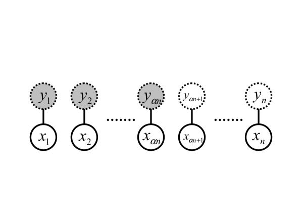
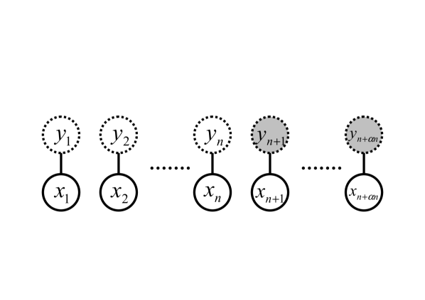
The goal of the present paper is to provide an error function for measuring the accuracy, which is suitable for the unsupervised learning with hierarchical models, and to derive its asymptotic form. For the first step, we consider the simplest case, in which the attributes, such as the range and dimension, of the latent variables are known; there is no singularity in the parameter space. This corresponds to the Reg-OV estimation in the table. Since the mathematical structure of the parameter is much more complicated in the singular case, we leave the analysis of the Sing-LV estimation for [Yamazaki12]. The main contributions of the present paper are the following three items: (1) estimation for the latent variables falls into three types as shown in Fig. 1 and their error functions are formulated in a distribution-based manner; (2) the asymptotic forms of the error functions are derived on the maximum likelihood and the Bayes methods in Type I and variants of Types II and III shown in Fig. 2; (3) it is determined that the Bayes method is more accurate than the maximum likelihood method in the asymptotic situation.

The rest of this paper is organized as follows: In Section 2 we explain the estimation of latent variables by comparing it with the prediction of observable variables. In Section 3 we provide the formal definitions of the estimation methods and the error functions. Section 4 then presents the main results for the asymptotic forms and the proofs. Discussions and conclusions are stated in Sections 5 and 6, respectively.

2 Estimations of Variables

This section distinguishes between the estimation of latent variables and the prediction of observable variables. There are variations on the estimation of latent variables due to the estimated targets.

Assume that the observable data and unobservable labels are represented by the observable variables x𝑥x and the latent variables y𝑦y, respectively. Let us define that xRM𝑥superscript𝑅𝑀x\in R^{M} and y{1,2,,K}𝑦12𝐾y\in\{1,2,\dots,K\}. In the case of a discrete x𝑥x such as x{1,2,,M}𝑥12𝑀x\in\{1,2,\dots,M\}, all the results in this paper hold if 𝑑xdifferential-d𝑥\int dx is replaced with x=1Msuperscriptsubscript𝑥1𝑀\sum_{x=1}^{M}. A set of n𝑛n independent data pairs is expressed as (Xn,Yn)={(x1,y1),,(xn,yn)}superscript𝑋𝑛superscript𝑌𝑛subscript𝑥1subscript𝑦1subscript𝑥𝑛subscript𝑦𝑛(X^{n},Y^{n})=\{(x_{1},y_{1}),\dots,(x_{n},y_{n})\}, where Xn={x1,,xn}superscript𝑋𝑛subscript𝑥1subscript𝑥𝑛X^{n}=\{x_{1},\dots,x_{n}\} and Yn={y1,,yn}superscript𝑌𝑛subscript𝑦1subscript𝑦𝑛Y^{n}=\{y_{1},\dots,y_{n}\}. More precisely, there is no dependency between xisubscript𝑥𝑖x_{i} and xjsubscript𝑥𝑗x_{j} or between yisubscript𝑦𝑖y_{i} and yjsubscript𝑦𝑗y_{j} for ij𝑖𝑗i\neq j.

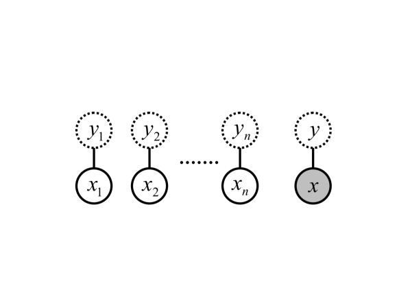
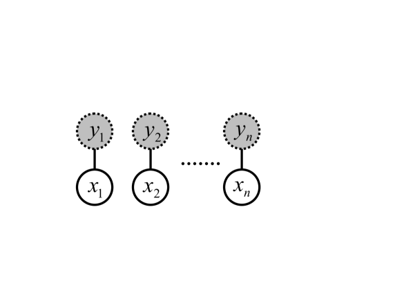
Refer to caption Prediction of observable variables Refer to caption Type I
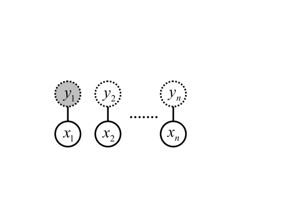
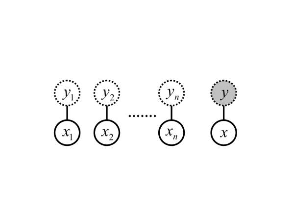
Refer to caption Type II Refer to caption Type III
Figure 1: Prediction of observable variables and estimations of latent variables. The observable data are {x1,,xn}subscript𝑥1subscript𝑥𝑛\{x_{1},\dots,x_{n}\}. Solid and dotted nodes are observable and unobservable, respectively. Gray nodes are estimation targets.

Figure 1 shows a variety of estimations of variables: prediction of an observable variable and three types of estimations of latent variables. Solid and dotted nodes are the observable and latent variables, respectively. A data pair is depicted by a connection between two nodes. The gray nodes are the target items of the estimations. We consider a stochastic approach, where the probability distribution of the target(s) is estimated from the training data Xnsuperscript𝑋𝑛X^{n}.

The top-left panel shows the prediction of unseen observable data. Based on Xnsuperscript𝑋𝑛X^{n}, the next observation x=xn+1𝑥subscript𝑥𝑛1x=x_{n+1} is predicted. The top-right panel shows the estimation of Ynsuperscript𝑌𝑛Y^{n}, which is referred to as Type I. In the stochastic approach, the joint probability of Ynsuperscript𝑌𝑛Y^{n} is estimated. The bottom-left panel shows marginal estimation, referred to as Type II. The marginal probability of yisubscript𝑦𝑖y_{i} (y1subscript𝑦1y_{1} is the example in the figure) is estimated; the rest of the latent variables in the probability are marginalized out. Note that there is no unseen/future data in either of Types I or II. The bottom-right panel shows estimation of y𝑦y in the unseen data, which is referred to as Type III. The difference between this and Type II is the training data; the corresponding observable part of the target is included in the training set in Type II, but it is not included in Type III. In the present paper we use a distribution-based approach to analyze the theoretical accuracy of a Type-I estimation, but we also consider connections to the other types.

3 Formal Definitions of Estimation Methods and Accuracy Evaluations

This section presents the maximum likelihood and Bayes methods for estimating latent variables and the corresponding error functions. Here, we consider only the Type-I estimation problem for the joint probability of the hidden part. The other types will be defined and discussed in Section 5.

Let p(x,y|w)=p(y|w)p(x|y,w)𝑝𝑥conditional𝑦𝑤𝑝conditional𝑦𝑤𝑝conditional𝑥𝑦𝑤p(x,y|w)=p(y|w)p(x|y,w) be a learning model, where wWRd𝑤𝑊superscript𝑅𝑑w\in W\subset R^{d} is the parameter. The probability of the observable data is expressed as

p(x|w)=𝑝conditional𝑥𝑤absent\displaystyle p(x|w)= y=1Kp(y|w)p(x|y,w).superscriptsubscript𝑦1𝐾𝑝conditional𝑦𝑤𝑝conditional𝑥𝑦𝑤\displaystyle\sum_{y=1}^{K}p(y|w)p(x|y,w).

Assume that the true model generating the data (Xn,Yn)superscript𝑋𝑛superscript𝑌𝑛(X^{n},Y^{n}) is expressed as q(x,y)=p(y|w)p(x|y,w)𝑞𝑥𝑦𝑝conditional𝑦superscript𝑤𝑝conditional𝑥𝑦superscript𝑤q(x,y)=p(y|w^{*})p(x|y,w^{*}), where wsuperscript𝑤w^{*} is the true parameter, and that the following Fisher information matrices exist and are positive definite;

{IXY(w)}ij=subscriptsubscript𝐼𝑋𝑌superscript𝑤𝑖𝑗absent\displaystyle\{I_{XY}(w^{*})\}_{ij}= E[lnp(x,y|w)wilnp(x,y|w)wj],𝐸delimited-[]𝑝𝑥conditional𝑦superscript𝑤subscript𝑤𝑖𝑝𝑥conditional𝑦superscript𝑤subscript𝑤𝑗\displaystyle E\biggl{[}\frac{\partial\ln p(x,y|w^{*})}{\partial w_{i}}\frac{\partial\ln p(x,y|w^{*})}{\partial w_{j}}\biggr{]},
{IX(w)}ij=subscriptsubscript𝐼𝑋superscript𝑤𝑖𝑗absent\displaystyle\{I_{X}(w^{*})\}_{ij}= E[lnp(x|w)wilnp(x|w)wj],𝐸delimited-[]𝑝conditional𝑥superscript𝑤subscript𝑤𝑖𝑝conditional𝑥superscript𝑤subscript𝑤𝑗\displaystyle E\biggl{[}\frac{\partial\ln p(x|w^{*})}{\partial w_{i}}\frac{\partial\ln p(x|w^{*})}{\partial w_{j}}\biggr{]},

where the expectation is

E[f(x,y)]=y=1Kf(x,y)p(x,y|w)dx.𝐸delimited-[]𝑓𝑥𝑦superscriptsubscript𝑦1𝐾𝑓𝑥𝑦𝑝𝑥conditional𝑦superscript𝑤𝑑𝑥\displaystyle E[f(x,y)]=\int\sum_{y=1}^{K}f(x,y)p(x,y|w^{*})dx.

This condition requires the identifiability of the true model, i.e., q(y)>0𝑞𝑦0q(y)>0 for all y𝑦y and ijq(x|y=i)q(x|y=j)𝑖𝑗𝑞conditional𝑥𝑦𝑖𝑞conditional𝑥𝑦𝑗i\neq j\Rightarrow q(x|y=i)\neq q(x|y=j). The joint probability distribution of (Xn,Yn)superscript𝑋𝑛superscript𝑌𝑛(X^{n},Y^{n}) is denoted by q(Xn,Yn)=i=1nq(xi,yi)𝑞superscript𝑋𝑛superscript𝑌𝑛superscriptsubscriptproduct𝑖1𝑛𝑞subscript𝑥𝑖subscript𝑦𝑖q(X^{n},Y^{n})=\prod_{i=1}^{n}q(x_{i},y_{i}).

We introduce two ways to construct a probability distribution of Ynsuperscript𝑌𝑛Y^{n} based on the observable Xnsuperscript𝑋𝑛X^{n}. First, we define an estimation method based on the maximum likelihood estimator. The likelihood is defined by

LX(w)=subscript𝐿𝑋𝑤absent\displaystyle L_{X}(w)= i=1np(xi|w).superscriptsubscriptproduct𝑖1𝑛𝑝conditionalsubscript𝑥𝑖𝑤\displaystyle\prod_{i=1}^{n}p(x_{i}|w).

The maximum likelihood estimator w^Xsubscript^𝑤𝑋\hat{w}_{X} is given by

w^X=subscript^𝑤𝑋absent\displaystyle\hat{w}_{X}= argmaxLX(w).subscript𝐿𝑋𝑤\displaystyle\arg\max L_{X}(w).
Definition 1 (The maximum likelihood method)

In the maximum likelihood estimation, the estimated distribution of the latent variables is defined by

p(Yn|Xn)=𝑝conditionalsuperscript𝑌𝑛superscript𝑋𝑛absent\displaystyle p(Y^{n}|X^{n})= p(Xn,Yn|w^X)Ynp(Xn,Yn|w^X)𝑝superscript𝑋𝑛conditionalsuperscript𝑌𝑛subscript^𝑤𝑋subscriptsuperscript𝑌𝑛𝑝superscript𝑋𝑛conditionalsuperscript𝑌𝑛subscript^𝑤𝑋\displaystyle\frac{p(X^{n},Y^{n}|\hat{w}_{X})}{\sum_{Y^{n}}p(X^{n},Y^{n}|\hat{w}_{X})}
=\displaystyle= i=1np(xi,yi|w^X)yip(xi,yi|w^X)=i=1np(yi|xi,w^X).superscriptsubscriptproduct𝑖1𝑛𝑝subscript𝑥𝑖conditionalsubscript𝑦𝑖subscript^𝑤𝑋subscriptsubscript𝑦𝑖𝑝subscript𝑥𝑖conditionalsubscript𝑦𝑖subscript^𝑤𝑋superscriptsubscriptproduct𝑖1𝑛𝑝conditionalsubscript𝑦𝑖subscript𝑥𝑖subscript^𝑤𝑋\displaystyle\prod_{i=1}^{n}\frac{p(x_{i},y_{i}|\hat{w}_{X})}{\sum_{y_{i}}p(x_{i},y_{i}|\hat{w}_{X})}=\prod_{i=1}^{n}p(y_{i}|x_{i},\hat{w}_{X}). (1)

The notation p(Yn|Xn,w^X)𝑝conditionalsuperscript𝑌𝑛superscript𝑋𝑛subscript^𝑤𝑋p(Y^{n}|X^{n},\hat{w}_{X}) is used when the method is emphasized.

Next, we define the Bayesian estimation. Let the likelihood of the joint probability distribution be

LXY(w)=subscript𝐿𝑋𝑌𝑤absent\displaystyle L_{XY}(w)= i=1np(xi,yi|w).superscriptsubscriptproduct𝑖1𝑛𝑝subscript𝑥𝑖conditionalsubscript𝑦𝑖𝑤\displaystyle\prod_{i=1}^{n}p(x_{i},y_{i}|w).

The marginal likelihood functions are given by

Z(Xn,Yn)=𝑍superscript𝑋𝑛superscript𝑌𝑛absent\displaystyle Z(X^{n},Y^{n})= LXY(w)φ(w;η)𝑑w,subscript𝐿𝑋𝑌𝑤𝜑𝑤𝜂differential-d𝑤\displaystyle\int L_{XY}(w)\varphi(w;\eta)dw,
Z(Xn)=𝑍superscript𝑋𝑛absent\displaystyle Z(X^{n})= YnZ(Xn,Yn)=LX(w)φ(w;η)𝑑w,subscriptsuperscript𝑌𝑛𝑍superscript𝑋𝑛superscript𝑌𝑛subscript𝐿𝑋𝑤𝜑𝑤𝜂differential-d𝑤\displaystyle\sum_{Y^{n}}Z(X^{n},Y^{n})=\int L_{X}(w)\varphi(w;\eta)dw,

where φ(w;η)𝜑𝑤𝜂\varphi(w;\eta) is a prior with the hyperparameter η𝜂\eta. We assume that the support of the prior includes wsuperscript𝑤w^{*}.

Definition 2 (The Bayes method)

In the Bayes estimation, the estimated distribution of Ynsuperscript𝑌𝑛Y^{n} is expressed as

p(Yn|Xn)=𝑝conditionalsuperscript𝑌𝑛superscript𝑋𝑛absent\displaystyle p(Y^{n}|X^{n})= Z(Xn,Yn)Z(Xn).𝑍superscript𝑋𝑛superscript𝑌𝑛𝑍superscript𝑋𝑛\displaystyle\frac{Z(X^{n},Y^{n})}{Z(X^{n})}. (2)

Based on the posterior distribution defined by

p(w|Xn)=1Z(Xn)LX(w)φ(w;η),𝑝conditional𝑤superscript𝑋𝑛1𝑍superscript𝑋𝑛subscript𝐿𝑋𝑤𝜑𝑤𝜂\displaystyle p(w|X^{n})=\frac{1}{Z(X^{n})}L_{X}(w)\varphi(w;\eta),

the estimated distribution has another equivalent form

p(Yn|Xn)=𝑝conditionalsuperscript𝑌𝑛superscript𝑋𝑛absent\displaystyle p(Y^{n}|X^{n})= i=1np(yi|xi,w)p(w|Xn)dw.superscriptsubscriptproduct𝑖1𝑛𝑝conditionalsubscript𝑦𝑖subscript𝑥𝑖𝑤𝑝conditional𝑤superscript𝑋𝑛𝑑𝑤\displaystyle\int\prod_{i=1}^{n}p(y_{i}|x_{i},w)p(w|X^{n})dw. (3)

Comparing Eq. 3 with Eq. 1 reveals that the Bayes estimation is based on the expectation over the posterior instead of the plug-in parameter w^Xsubscript^𝑤𝑋\hat{w}_{X}.

The distribution of Ynsuperscript𝑌𝑛Y^{n} in the true model is uniquely expressed as

q(Yn|Xn)=i=1nq(yi|xi)=i=1nq(xi,yi)q(xi),𝑞conditionalsuperscript𝑌𝑛superscript𝑋𝑛superscriptsubscriptproduct𝑖1𝑛𝑞conditionalsubscript𝑦𝑖subscript𝑥𝑖superscriptsubscriptproduct𝑖1𝑛𝑞subscript𝑥𝑖subscript𝑦𝑖𝑞subscript𝑥𝑖\displaystyle q(Y^{n}|X^{n})=\prod_{i=1}^{n}q(y_{i}|x_{i})=\prod_{i=1}^{n}\frac{q(x_{i},y_{i})}{q(x_{i})},

where q(xi)=yi=1Kq(xi,yi)𝑞subscript𝑥𝑖superscriptsubscriptsubscript𝑦𝑖1𝐾𝑞subscript𝑥𝑖subscript𝑦𝑖q(x_{i})=\sum_{y_{i}=1}^{K}q(x_{i},y_{i}). Accuracy of the latent variable estimation is measured by the difference between the true distribution q(Yn|Xn)𝑞conditionalsuperscript𝑌𝑛superscript𝑋𝑛q(Y^{n}|X^{n}) and the estimated one p(Yn|Xn)𝑝conditionalsuperscript𝑌𝑛superscript𝑋𝑛p(Y^{n}|X^{n}). For the present paper, we define the error function as the average Kullback-Leibler divergence,

D(n)=𝐷𝑛absent\displaystyle D(n)= 1nEXn[Ynq(Yn|Xn)lnq(Yn|Xn)p(Yn|Xn)],1𝑛subscript𝐸superscript𝑋𝑛delimited-[]subscriptsuperscript𝑌𝑛𝑞conditionalsuperscript𝑌𝑛superscript𝑋𝑛𝑞conditionalsuperscript𝑌𝑛superscript𝑋𝑛𝑝conditionalsuperscript𝑌𝑛superscript𝑋𝑛\displaystyle\frac{1}{n}E_{X^{n}}\biggl{[}\sum_{Y^{n}}q(Y^{n}|X^{n})\ln\frac{q(Y^{n}|X^{n})}{p(Y^{n}|X^{n})}\biggr{]}, (4)

where the expectation is

EXn[f(Xn)]=subscript𝐸superscript𝑋𝑛delimited-[]𝑓superscript𝑋𝑛absent\displaystyle E_{X^{n}}[f(X^{n})]= f(Xn)q(Xn)𝑑Xn.𝑓superscript𝑋𝑛𝑞superscript𝑋𝑛differential-dsuperscript𝑋𝑛\displaystyle\int f(X^{n})q(X^{n})dX^{n}.

Note that this function is available for any construction of p(Yn|Xn)𝑝conditionalsuperscript𝑌𝑛superscript𝑋𝑛p(Y^{n}|X^{n}) when we consider the cases of the maximum likelihood and the Bayes methods below.

4 Asymptotic Analysis of the Error Function

In this section we present the main theorems for the asymptotic forms of the error function.

4.1 Asymptotic Errors of the Two Methods

In the unsupervised learning, there is label switching, which makes interpretation of the estimation result difficult. For example, define the parameter wssubscriptsuperscript𝑤𝑠w^{*}_{s} as p(x,y=1|ws)=p(x,y=2|w)𝑝𝑥𝑦conditional1subscriptsuperscript𝑤𝑠𝑝𝑥𝑦conditional2superscript𝑤p(x,y=1|w^{*}_{s})=p(x,y=2|w^{*}), p(x,y=2|ws)=p(x,y=1|w)𝑝𝑥𝑦conditional2subscriptsuperscript𝑤𝑠𝑝𝑥𝑦conditional1superscript𝑤p(x,y=2|w^{*}_{s})=p(x,y=1|w^{*}), and p(x,y=k|ws)=p(x,y=k|w)𝑝𝑥𝑦conditional𝑘subscriptsuperscript𝑤𝑠𝑝𝑥𝑦conditional𝑘superscript𝑤p(x,y=k|w^{*}_{s})=p(x,y=k|w^{*}) for k>2𝑘2k>2. In this parameter, the label y=1𝑦1y=1 and y=2𝑦2y=2 are switched compared with wsuperscript𝑤w^{*}. It holds that p(x|ws)=p(x|w)𝑝conditional𝑥subscriptsuperscript𝑤𝑠𝑝conditional𝑥superscript𝑤p(x|w^{*}_{s})=p(x|w^{*}) whereas p(x,y|ws)p(x,y|w)𝑝𝑥conditional𝑦subscriptsuperscript𝑤𝑠𝑝𝑥conditional𝑦superscript𝑤p(x,y|w^{*}_{s})\neq p(x,y|w^{*}). Therefore, the estimation methods can search for wssubscriptsuperscript𝑤𝑠w^{*}_{s} as the true parameter instead of wsuperscript𝑤w^{*} since there is no information of the true labels. In the present paper, we focus on the best performance, where we successfully estimate the true parameter. In other words, we define the true parameter according to the estimated label assignment. Under the best performance situation, the maximum likelihood estimator w^Xsubscript^𝑤𝑋\hat{w}_{X} converges to wsuperscript𝑤w^{*} in probability, and the posterior distribution of the Bayes method converges to the normal distribution, the mean of which is w^Xsubscript^𝑤𝑋\hat{w}_{X}, in law. Then, it is obvious that the error function D(n)𝐷𝑛D(n) goes to zero at n𝑛n\rightarrow\infty.

The following theorems show the speed of decrease of the error function;

Theorem 3 (The asymptotic error of the maximum likelihood method)

In the latent variable estimation given by Eq.1, the error function Eq.4 has the following asymptotic form:

D(n)=𝐷𝑛absent\displaystyle D(n)= 12nTr[{IXY(w)IX(w)}IX1(w)]+o(1n).12𝑛Trdelimited-[]subscript𝐼𝑋𝑌superscript𝑤subscript𝐼𝑋superscript𝑤subscriptsuperscript𝐼1𝑋superscript𝑤𝑜1𝑛\displaystyle\frac{1}{2n}\mathrm{Tr}[\{I_{XY}(w^{*})-I_{X}(w^{*})\}I^{-1}_{X}(w^{*})]+o\bigg{(}\frac{1}{n}\bigg{)}.
Theorem 4 (The asymptotic error of the Bayes method)

In the latent variable estimation given by Eq.2, the error function Eq.4 has the following asymptotic form:

D(n)=𝐷𝑛absent\displaystyle D(n)= 12nlndet[IXY(w)IX1(w)]+o(1n).12𝑛delimited-[]subscript𝐼𝑋𝑌superscript𝑤subscriptsuperscript𝐼1𝑋superscript𝑤𝑜1𝑛\displaystyle\frac{1}{2n}\ln\det\big{[}I_{XY}(w^{*})I^{-1}_{X}(w^{*})\big{]}+o\bigg{(}\frac{1}{n}\bigg{)}.

The proofs are in the appendix. The dominant order is 1/n1𝑛1/n in both methods, and its coefficient depends on the Fisher information matrices. It is not an unaccountable result that the error value depends on the position of wsuperscript𝑤w^{*}. For example, let us consider cluster analysis and assume that distances among the clusters are large. Since we can easily distinguish the clusters, there is not much additional information on the label y𝑦y. Then, IXY(w)subscript𝐼𝑋𝑌superscript𝑤I_{XY}(w^{*}) is close to IX(w)subscript𝐼𝑋superscript𝑤I_{X}(w^{*}), which makes D(n)𝐷𝑛D(n) small in both methods. The true parameter generally determines difficulty of tasks in the unsupervised learning, and the theorems reflect this fact. We will present a more detailed discussion on the coefficient in Section 5.

The following corollary shows the advantage of the Bayes estimation.

Corollary 5

Let the error functions for the maximum likelihood and the Bayes methods be denoted by DML(n)superscript𝐷ML𝑛D^{\text{ML}}(n) and DBayes(n)superscript𝐷Bayes𝑛D^{\text{Bayes}}(n), respectively. Assume that IXY(w)IX(w)subscript𝐼𝑋𝑌superscript𝑤subscript𝐼𝑋superscript𝑤I_{XY}(w^{*})\neq I_{X}(w^{*}). For any true parameter wsuperscript𝑤w^{*}, there exists a positive constant c𝑐c such that

DML(n)DBayes(n)cn+o(1n).superscript𝐷ML𝑛superscript𝐷Bayes𝑛𝑐𝑛𝑜1𝑛\displaystyle D^{\text{ML}}(n)-D^{\text{Bayes}}(n)\geq\frac{c}{n}+o\bigg{(}\frac{1}{n}\bigg{)}.

The proof is in the appendix. This result shows that DML(n)>DBayes(n)superscript𝐷ML𝑛superscript𝐷Bayes𝑛D^{\text{ML}}(n)>D^{\text{Bayes}}(n) for a sufficiently large data size n𝑛n.

5 Discussion

5.1 Relation to Other Error Functions

We now formulate the predictions of observable data and the remaining estimations for Types II and III, and we consider the relations of their error functions to that of Type I.

First, we compare the Reg-LV estimation with the Reg-OV estimation. In the observable-variable estimation, the error function is referred to as the generalization error, which measures the prediction performance on unseen observable data. The generalization error is defined as

Dx(n)=subscript𝐷𝑥𝑛absent\displaystyle D_{x}(n)= EXn[q(x)lnq(x)p(x|Xn)dx],subscript𝐸superscript𝑋𝑛delimited-[]𝑞𝑥𝑞𝑥𝑝conditional𝑥superscript𝑋𝑛𝑑𝑥\displaystyle E_{X^{n}}\bigg{[}\int q(x)\ln\frac{q(x)}{p(x|X^{n})}dx\bigg{]},

where x𝑥x is independent of Xnsuperscript𝑋𝑛X^{n} in the data-generating process of q(x)𝑞𝑥q(x). The predictive distribution p(x|Xn)𝑝conditional𝑥superscript𝑋𝑛p(x|X^{n}) is constructed by

p(x|Xn)=𝑝conditional𝑥superscript𝑋𝑛absent\displaystyle p(x|X^{n})= p(x|w^X)𝑝conditional𝑥subscript^𝑤𝑋\displaystyle p(x|\hat{w}_{X})

for the maximum likelihood method and

p(x|Xn)=𝑝conditional𝑥superscript𝑋𝑛absent\displaystyle p(x|X^{n})= p(x|w)p(w|Xn)𝑑w𝑝conditional𝑥𝑤𝑝conditional𝑤superscript𝑋𝑛differential-d𝑤\displaystyle\int p(x|w)p(w|X^{n})dw

for the Bayes method. Both methods estimation have the same dominant terms in their asymptotic forms,

Dx(n)=subscript𝐷𝑥𝑛absent\displaystyle D_{x}(n)= d2n+o(1n).𝑑2𝑛𝑜1𝑛\displaystyle\frac{d}{2n}+o\bigg{(}\frac{1}{n}\bigg{)}.

The coefficient of the asymptotic generalization error depends only on the dimension of the parameter for any model, but that of D(n)𝐷𝑛D(n) is determined by both the model expression and the true parameter wsuperscript𝑤w^{*}. This dependency appears when the learning model does not contain the true model in the Reg-OV estimation, and w^Xsubscript^𝑤𝑋\hat{w}_{X} is used for approximation of the error function for model selection [Takeuchi1976] and active learning [book:Fedorov:1972]. In the same way, by replacing wsuperscript𝑤w^{*} with w^Xsubscript^𝑤𝑋\hat{w}_{X}, Theorems 3 and 4 enable us to calculate the error function in the Reg-LV estimation.

In the observable-variable estimation, the error Dx(n)subscript𝐷𝑥𝑛D_{x}(n) is approximated by the cross-validation and bootstrap methods since unseen data xn+1subscript𝑥𝑛1x_{n+1} are interchangeable with one of the given observable data. On the other hand, there is no substitution for the latent variable, which means that any numerical approximation does not exist for D(n)𝐷𝑛D(n) in principle. The theoretical results in the present paper are thus far the only way to estimate the accuracy.

Next, we discuss Type-II estimation; we focus on the value yisubscript𝑦𝑖y_{i} from Ynsuperscript𝑌𝑛Y^{n} and its estimation accuracy. Based on the joint probability, the estimation of yisubscript𝑦𝑖y_{i} is defined by

p(yi|Xn)=𝑝conditionalsubscript𝑦𝑖superscript𝑋𝑛absent\displaystyle p(y_{i}|X^{n})= Yn\yip(Yn|Xn),subscript\superscript𝑌𝑛subscript𝑦𝑖𝑝conditionalsuperscript𝑌𝑛superscript𝑋𝑛\displaystyle\sum_{Y^{n}\backslash y_{i}}p(Y^{n}|X^{n}),

where the summation is taken over Ynsuperscript𝑌𝑛Y^{n} except for yisubscript𝑦𝑖y_{i}. Thus the error function depends on which yisubscript𝑦𝑖y_{i} we exclude. In order to measure the average effect of the exclusions, we define the error as follows:

Dy|Xn(n)=subscript𝐷conditional𝑦superscript𝑋𝑛𝑛absent\displaystyle D_{y|X^{n}}(n)= EXn[1ni=1nyiq(yi|xi)lnq(yi|xi)p(yi|Xn)].subscript𝐸superscript𝑋𝑛delimited-[]1𝑛superscriptsubscript𝑖1𝑛subscriptsubscript𝑦𝑖𝑞conditionalsubscript𝑦𝑖subscript𝑥𝑖𝑞conditionalsubscript𝑦𝑖subscript𝑥𝑖𝑝conditionalsubscript𝑦𝑖superscript𝑋𝑛\displaystyle E_{X^{n}}\bigg{[}\frac{1}{n}\sum_{i=1}^{n}\sum_{y_{i}}q(y_{i}|x_{i})\ln\frac{q(y_{i}|x_{i})}{p(y_{i}|X^{n})}\bigg{]}.

The maximum likelihood method has the following estimation,

p(yi|Xn)=𝑝conditionalsubscript𝑦𝑖superscript𝑋𝑛absent\displaystyle p(y_{i}|X^{n})= Yn\yii=1np(xi,yi|w^X)p(xi|w^X)subscript\superscript𝑌𝑛subscript𝑦𝑖superscriptsubscriptproduct𝑖1𝑛𝑝subscript𝑥𝑖conditionalsubscript𝑦𝑖subscript^𝑤𝑋𝑝conditionalsubscript𝑥𝑖subscript^𝑤𝑋\displaystyle\sum_{Y^{n}\backslash y_{i}}\prod_{i=1}^{n}\frac{p(x_{i},y_{i}|\hat{w}_{X})}{p(x_{i}|\hat{w}_{X})}
=\displaystyle= p(x1|w^X)p(xi1|w^X)p(xi,yi|w^X)p(xi+1|w^X)p(xn|w^X)i=1np(xi|w^X)𝑝conditionalsubscript𝑥1subscript^𝑤𝑋𝑝conditionalsubscript𝑥𝑖1subscript^𝑤𝑋𝑝subscript𝑥𝑖conditionalsubscript𝑦𝑖subscript^𝑤𝑋𝑝conditionalsubscript𝑥𝑖1subscript^𝑤𝑋𝑝conditionalsubscript𝑥𝑛subscript^𝑤𝑋superscriptsubscriptproduct𝑖1𝑛𝑝conditionalsubscript𝑥𝑖subscript^𝑤𝑋\displaystyle\frac{p(x_{1}|\hat{w}_{X})\cdots p(x_{i-1}|\hat{w}_{X})p(x_{i},y_{i}|\hat{w}_{X})p(x_{i+1}|\hat{w}_{X})\cdots p(x_{n}|\hat{w}_{X})}{\prod_{i=1}^{n}p(x_{i}|\hat{w}_{X})}
=\displaystyle= p(xi,yi|w^X)p(xi|w^X)=p(yi|xi,w^X).𝑝subscript𝑥𝑖conditionalsubscript𝑦𝑖subscript^𝑤𝑋𝑝conditionalsubscript𝑥𝑖subscript^𝑤𝑋𝑝conditionalsubscript𝑦𝑖subscript𝑥𝑖subscript^𝑤𝑋\displaystyle\frac{p(x_{i},y_{i}|\hat{w}_{X})}{p(x_{i}|\hat{w}_{X})}=p(y_{i}|x_{i},\hat{w}_{X}).

We can easily find that

Dy|Xn(n)=subscript𝐷conditional𝑦superscript𝑋𝑛𝑛absent\displaystyle D_{y|X^{n}}(n)= EXn[1ni=1nyi=1Kq(yi|xi)lnq(yi|xi)p(yi|xi,w^X)]subscript𝐸superscript𝑋𝑛delimited-[]1𝑛superscriptsubscript𝑖1𝑛superscriptsubscriptsubscript𝑦𝑖1𝐾𝑞conditionalsubscript𝑦𝑖subscript𝑥𝑖𝑞conditionalsubscript𝑦𝑖subscript𝑥𝑖𝑝conditionalsubscript𝑦𝑖subscript𝑥𝑖subscript^𝑤𝑋\displaystyle E_{X^{n}}\bigg{[}\frac{1}{n}\sum_{i=1}^{n}\sum_{y_{i}=1}^{K}q(y_{i}|x_{i})\ln\frac{q(y_{i}|x_{i})}{p(y_{i}|x_{i},\hat{w}_{X})}\bigg{]}
=\displaystyle= 1nEXn[Ynq(Yn|Xn)lnq(Yn|Xn)p(Yn|Xn,w^X)].1𝑛subscript𝐸superscript𝑋𝑛delimited-[]subscriptsuperscript𝑌𝑛𝑞conditionalsuperscript𝑌𝑛superscript𝑋𝑛𝑞conditionalsuperscript𝑌𝑛superscript𝑋𝑛𝑝conditionalsuperscript𝑌𝑛superscript𝑋𝑛subscript^𝑤𝑋\displaystyle\frac{1}{n}E_{X^{n}}\bigg{[}\sum_{Y^{n}}q(Y^{n}|X^{n})\ln\frac{q(Y^{n}|X^{n})}{p(Y^{n}|X^{n},\hat{w}_{X})}\bigg{]}.

Therefore, it holds that Dy|Xn(n)=D(n)subscript𝐷conditional𝑦superscript𝑋𝑛𝑛𝐷𝑛D_{y|X^{n}}(n)=D(n) in the maximum likelihood method. However, the Bayes method has the estimation,

p(yi|Xn)=𝑝conditionalsubscript𝑦𝑖superscript𝑋𝑛absent\displaystyle p(y_{i}|X^{n})= p(x1|w)p(xi1|w)p(xi,yi|w)p(xi+1|w)p(xn|w)φ(w;η)𝑑wZ(Xn),𝑝conditionalsubscript𝑥1𝑤𝑝conditionalsubscript𝑥𝑖1𝑤𝑝subscript𝑥𝑖conditionalsubscript𝑦𝑖𝑤𝑝conditionalsubscript𝑥𝑖1𝑤𝑝conditionalsubscript𝑥𝑛𝑤𝜑𝑤𝜂differential-d𝑤𝑍superscript𝑋𝑛\displaystyle\frac{\int p(x_{1}|w)\cdots p(x_{i-1}|w)p(x_{i},y_{i}|w)p(x_{i+1}|w)\cdots p(x_{n}|w)\varphi(w;\eta)dw}{Z(X^{n})},

which indicates Dy|Xn(n)D(n)subscript𝐷conditional𝑦superscript𝑋𝑛𝑛𝐷𝑛D_{y|X^{n}}(n)\neq D(n). A sufficient condition for Dy|Xn(n)=D(n)subscript𝐷conditional𝑦superscript𝑋𝑛𝑛𝐷𝑛D_{y|X^{n}}(n)=D(n) is to satisfy p(Yn|Xn)=i=1np(yi|Xn)𝑝conditionalsuperscript𝑌𝑛superscript𝑋𝑛superscriptsubscriptproduct𝑖1𝑛𝑝conditionalsubscript𝑦𝑖superscript𝑋𝑛p(Y^{n}|X^{n})=\prod_{i=1}^{n}p(y_{i}|X^{n}).

Finally, we consider the Type-III estimation. The error is defined by

Dy|x(n)=subscript𝐷conditional𝑦𝑥𝑛absent\displaystyle D_{y|x}(n)= EXn[q(x)y=1Kq(y|x)lnq(y|x)p(y|x,Xn)dx].subscript𝐸superscript𝑋𝑛delimited-[]𝑞𝑥superscriptsubscript𝑦1𝐾𝑞conditional𝑦𝑥𝑞conditional𝑦𝑥𝑝conditional𝑦𝑥superscript𝑋𝑛𝑑𝑥\displaystyle E_{X^{n}}\bigg{[}\int q(x)\sum_{y=1}^{K}q(y|x)\ln\frac{q(y|x)}{p(y|x,X^{n})}dx\bigg{]}.

Note that the new observation x𝑥x is not used for estimation of y𝑦y, or Dy|x(n)subscript𝐷conditional𝑦𝑥𝑛D_{y|x}(n) will be equivalent to the Type-II error Dy|Xn+1(n+1)subscript𝐷conditional𝑦superscript𝑋𝑛1𝑛1D_{y|X^{n+1}}(n+1). The maximum likelihood estimation p(y|x,Xn)𝑝conditional𝑦𝑥superscript𝑋𝑛p(y|x,X^{n}) is given by

p(y|x,Xn)=𝑝conditional𝑦𝑥superscript𝑋𝑛absent\displaystyle p(y|x,X^{n})= p(x,y|w^X)p(x|w^X),𝑝𝑥conditional𝑦subscript^𝑤𝑋𝑝conditional𝑥subscript^𝑤𝑋\displaystyle\frac{p(x,y|\hat{w}_{X})}{p(x|\hat{w}_{X})},

and for the Bayes method it is

p(y|x,Xn)=𝑝conditional𝑦𝑥superscript𝑋𝑛absent\displaystyle p(y|x,X^{n})= p(x,y|w)p(x|w)p(w|Xn)𝑑w.𝑝𝑥conditional𝑦𝑤𝑝conditional𝑥𝑤𝑝conditional𝑤superscript𝑋𝑛differential-d𝑤\displaystyle\int\frac{p(x,y|w)}{p(x|w)}p(w|X^{n})dw. (5)

Using the result in [ShimodairaPDOI] for a variant Akaike information criterion (AIC) from partially observed data, we immediately obtain the asymptotic form of Dy|x(n)subscript𝐷conditional𝑦𝑥𝑛D_{y|x}(n) as

Dy|x(n)=subscript𝐷conditional𝑦𝑥𝑛absent\displaystyle D_{y|x}(n)= 12nTr[{IXY(w)IX(w)}IX(w)1]+o(1n).12𝑛Trdelimited-[]subscript𝐼𝑋𝑌superscript𝑤subscript𝐼𝑋superscript𝑤subscript𝐼𝑋superscriptsuperscript𝑤1𝑜1𝑛\displaystyle\frac{1}{2n}\mathrm{Tr}\bigg{[}\bigg{\{}I_{XY}(w^{*})-I_{X}(w^{*})\bigg{\}}I_{X}(w^{*})^{-1}\bigg{]}+o\bigg{(}\frac{1}{n}\bigg{)}.

We thus conclude that all estimation types have the same accuracy in the maximum likelihood method. The difference of the training data between Types II and III does not asymptotically affect the estimation results. The analysis of the Type-III estimate in the Bayes method is left for future study.

5.2 Variants of Types II and III

Table 2: Coefficients of the dominant order 1/n1𝑛1/n in the error functions
Prediction Type I Type II Type III
ML d/2𝑑2d/2 Tr[{IXYIX}IX1]/2Trdelimited-[]subscript𝐼𝑋𝑌subscript𝐼𝑋superscriptsubscript𝐼𝑋12\mathrm{Tr}[\{I_{XY}-I_{X}\}I_{X}^{-1}]/2 Tr[{IXYIX}IX1]/2Trdelimited-[]subscript𝐼𝑋𝑌subscript𝐼𝑋superscriptsubscript𝐼𝑋12\mathrm{Tr}[\{I_{XY}-I_{X}\}I_{X}^{-1}]/2 Tr[{IXYIX}IX1]/2Trdelimited-[]subscript𝐼𝑋𝑌subscript𝐼𝑋superscriptsubscript𝐼𝑋12\mathrm{Tr}[\{I_{XY}-I_{X}\}I_{X}^{-1}]/2
Bayes d/2𝑑2d/2 lndet[IXYIX1]/2delimited-[]subscript𝐼𝑋𝑌superscriptsubscript𝐼𝑋12\ln\det[I_{XY}I_{X}^{-1}]/2 unknown unknown

Table 2 summarizes the results in the previous subsection. The rows indicate the maximum likelihood (ML) and the Bayes methods, respectively. The Fisher information matrices IXY(w)subscript𝐼𝑋𝑌superscript𝑤I_{XY}(w^{*}) and IX(w)subscript𝐼𝑋superscript𝑤I_{X}(w^{*}) are abbreviated in a form that does not include the true parameter, i.e., IXYsubscript𝐼𝑋𝑌I_{XY} and IXsubscript𝐼𝑋I_{X}. The error functions of Types II and III in the Bayes method are still unknown. The analysis is not straightforward when there is a single target of estimation, because the asymptotic expansion is not available when the number of target nodes is constant with respect to the training data size n𝑛n.

Refer to caption Type II’ Refer to caption Type III’
Figure 2: (Left) Partial marginal estimation for y1,,yαnsubscript𝑦1subscript𝑦𝛼𝑛y_{1},\dots,y_{\alpha n}. (Right) Estimation for future data yn+1,,yn+αnsubscript𝑦𝑛1subscript𝑦𝑛𝛼𝑛y_{n+1},\dots,y_{n+\alpha n}.

Consider the variants of Types II and III depicted in Figure 2. Assume that 0<α10𝛼10<\alpha\leq 1 is a constant rational number and that n𝑛n gets large enough to satisfy that αn𝛼𝑛\alpha n is an integer. The left panel shows the partial marginal estimation referred to as Type II’. We will consider the joint probability of y1,,yαnsubscript𝑦1subscript𝑦𝛼𝑛y_{1},\dots,y_{\alpha n}, where the remaining variables yαn+1,,ynsubscript𝑦𝛼𝑛1subscript𝑦𝑛y_{\alpha n+1},\dots,y_{n} have been marginalized out. Type II’ is equivalent to Type I when α=1𝛼1\alpha=1. Note that the order in which the target nodes are determined does not change the average accuracy for i.i.d. data. The right panel indicates the estimations for future data yn+1,,yn+αnsubscript𝑦𝑛1subscript𝑦𝑛𝛼𝑛y_{n+1},\dots,y_{n+\alpha n}. We refer to it as Type III’ and construct the joint probability on these variables. In the variant types, the targets are changed from a single node to αn𝛼𝑛\alpha n nodes, which enables us to analyze the asymptotic behavior.

We will use the following notation:

X1=subscript𝑋1absent\displaystyle X_{1}= {x1,,xαn},subscript𝑥1subscript𝑥𝛼𝑛\displaystyle\{x_{1},\dots,x_{\alpha n}\},
Y1=subscript𝑌1absent\displaystyle Y_{1}= {y1,,yαn}subscript𝑦1subscript𝑦𝛼𝑛\displaystyle\{y_{1},\dots,y_{\alpha n}\}

for Type II’ and

X2=subscript𝑋2absent\displaystyle X_{2}= {xn+1,,xn+αn},subscript𝑥𝑛1subscript𝑥𝑛𝛼𝑛\displaystyle\{x_{n+1},\dots,x_{n+\alpha n}\},
Y2=subscript𝑌2absent\displaystyle Y_{2}= {yn+1,,yn+αn}subscript𝑦𝑛1subscript𝑦𝑛𝛼𝑛\displaystyle\{y_{n+1},\dots,y_{n+\alpha n}\}

for Type III’. The Bayes estimations are given by

p(Y1|Xn)=𝑝conditionalsubscript𝑌1superscript𝑋𝑛absent\displaystyle p(Y_{1}|X^{n})= j=1αnp(xj,yj|w)i=αn+1np(xi|w)φ(w;η)dwi=1np(xi|w)φ(w;η)dw,superscriptsubscriptproduct𝑗1𝛼𝑛𝑝subscript𝑥𝑗conditionalsubscript𝑦𝑗𝑤superscriptsubscriptproduct𝑖𝛼𝑛1𝑛𝑝conditionalsubscript𝑥𝑖𝑤𝜑𝑤𝜂𝑑𝑤superscriptsubscriptproduct𝑖1𝑛𝑝conditionalsubscript𝑥𝑖𝑤𝜑𝑤𝜂𝑑𝑤\displaystyle\frac{\int\prod_{j=1}^{\alpha n}p(x_{j},y_{j}|w)\prod_{i=\alpha n+1}^{n}p(x_{i}|w)\varphi(w;\eta)dw}{\int\prod_{i=1}^{n}p(x_{i}|w)\varphi(w;\eta)dw},
p(Y2|X2,Xn)=𝑝conditionalsubscript𝑌2subscript𝑋2superscript𝑋𝑛absent\displaystyle p(Y_{2}|X_{2},X^{n})= i=n+1n+αnp(xi,yi|w)p(xi|w)p(w|Xn)dwsuperscriptsubscriptproduct𝑖𝑛1𝑛𝛼𝑛𝑝subscript𝑥𝑖conditionalsubscript𝑦𝑖𝑤𝑝conditionalsubscript𝑥𝑖𝑤𝑝conditional𝑤superscript𝑋𝑛𝑑𝑤\displaystyle\int\prod_{i=n+1}^{n+\alpha n}\frac{p(x_{i},y_{i}|w)}{p(x_{i}|w)}p(w|X^{n})dw

for Type II’ and Type III’, respectively. The respective error functions are defined by

DY1|Xn(n)=subscript𝐷conditionalsubscript𝑌1superscript𝑋𝑛𝑛absent\displaystyle D_{Y_{1}|X^{n}}(n)= 1αnEXn[Y1q(Y1|Xn)lnq(Y1|Xn)p(Y1|Xn)],1𝛼𝑛subscript𝐸superscript𝑋𝑛delimited-[]subscriptsubscript𝑌1𝑞conditionalsubscript𝑌1superscript𝑋𝑛𝑞conditionalsubscript𝑌1superscript𝑋𝑛𝑝conditionalsubscript𝑌1superscript𝑋𝑛\displaystyle\frac{1}{\alpha n}E_{X^{n}}\bigg{[}\sum_{Y_{1}}q(Y_{1}|X^{n})\ln\frac{q(Y_{1}|X^{n})}{p(Y_{1}|X^{n})}\bigg{]},
DY2|X2(n)=subscript𝐷conditionalsubscript𝑌2subscript𝑋2𝑛absent\displaystyle D_{Y_{2}|X_{2}}(n)= 1αnEXn,X2[Y2q(Y2|X2)lnq(Y2|X2)p(Y2|X2,Xn)].1𝛼𝑛subscript𝐸superscript𝑋𝑛subscript𝑋2delimited-[]subscriptsubscript𝑌2𝑞conditionalsubscript𝑌2subscript𝑋2𝑞conditionalsubscript𝑌2subscript𝑋2𝑝conditionalsubscript𝑌2subscript𝑋2superscript𝑋𝑛\displaystyle\frac{1}{\alpha n}E_{X^{n},X_{2}}\bigg{[}\sum_{Y_{2}}q(Y_{2}|X_{2})\ln\frac{q(Y_{2}|X_{2})}{p(Y_{2}|X_{2},X^{n})}\bigg{]}.

In ways similar to the proofs of Theorems 3 and 4, the asymptotic forms are derived as follows.

Theorem 6

In Type II’, the error function has the following asymptotic form:

DY1|Xn(n)=subscript𝐷conditionalsubscript𝑌1superscript𝑋𝑛𝑛absent\displaystyle D_{Y_{1}|X^{n}}(n)= 12αnlndet[KXY(w)IX(w)1]+o(1n),12𝛼𝑛delimited-[]subscript𝐾𝑋𝑌superscript𝑤subscript𝐼𝑋superscriptsuperscript𝑤1𝑜1𝑛\displaystyle\frac{1}{2\alpha n}\ln\det[K_{XY}(w^{*})I_{X}(w^{*})^{-1}]+o\bigg{(}\frac{1}{n}\bigg{)},

where KXY(w)=αIXY(w)+(1α)IX(w)subscript𝐾𝑋𝑌𝑤𝛼subscript𝐼𝑋𝑌𝑤1𝛼subscript𝐼𝑋𝑤K_{XY}(w)=\alpha I_{XY}(w)+(1-\alpha)I_{X}(w).

The proof is in the appendix.

Theorem 7

In Type III’, the error function has the following asymptotic form:

DY2|X2(n)=subscript𝐷conditionalsubscript𝑌2subscript𝑋2𝑛absent\displaystyle D_{Y_{2}|X_{2}}(n)= 12αnlndet[KXY(w)IX1(w)]+o(1n).12𝛼𝑛delimited-[]subscript𝐾𝑋𝑌superscript𝑤superscriptsubscript𝐼𝑋1superscript𝑤𝑜1𝑛\displaystyle\frac{1}{2\alpha n}\ln\det[K_{XY}(w^{*})I_{X}^{-1}(w^{*})]+o\bigg{(}\frac{1}{n}\bigg{)}.

This proof is also in the appendix. These theorems show that when Types II’ and III’ have the same α𝛼\alpha, they asymptotically have the same accuracy. This implies the asymptotic equivalency of Types II and III by combining the results of the maximum likelihood method.

Table 3: Coefficients of the dominant order 1/n1𝑛1/n in the error functions
Pred. Type I Type II’ Type III’
ML d/2𝑑2d/2 Tr[{IXYIX}IX1]/2Trdelimited-[]subscript𝐼𝑋𝑌subscript𝐼𝑋superscriptsubscript𝐼𝑋12\mathrm{Tr}[\{I_{XY}-I_{X}\}I_{X}^{-1}]/2 Tr[{IXYIX}IX1]/2Trdelimited-[]subscript𝐼𝑋𝑌subscript𝐼𝑋superscriptsubscript𝐼𝑋12\mathrm{Tr}[\{I_{XY}-I_{X}\}I_{X}^{-1}]/2 Tr[{IXYIX}IX1]/2Trdelimited-[]subscript𝐼𝑋𝑌subscript𝐼𝑋superscriptsubscript𝐼𝑋12\mathrm{Tr}[\{I_{XY}-I_{X}\}I_{X}^{-1}]/2
Bayes d/2𝑑2d/2 lndet[IXYIX1]/2delimited-[]subscript𝐼𝑋𝑌superscriptsubscript𝐼𝑋12\ln\det[I_{XY}I_{X}^{-1}]/2 lndet[KXYIX1]/(2α)delimited-[]subscript𝐾𝑋𝑌superscriptsubscript𝐼𝑋12𝛼\ln\det[K_{XY}I_{X}^{-1}]/(2\alpha) lndet[KXYIX1]/(2α)delimited-[]subscript𝐾𝑋𝑌superscriptsubscript𝐼𝑋12𝛼\ln\det[K_{XY}I_{X}^{-1}]/(2\alpha)

Table 3 summarizes the results. Based on the definitions, the results for the maximum likelihood method are also available for Types II’ and III’. Using the asymptotic forms, we can compare the relation of the magnitudes for the maximum likelihood method.

Corollary 8

Assume that IXY(w)IX(w)subscript𝐼𝑋𝑌𝑤subscript𝐼𝑋𝑤I_{XY}(w)\neq I_{X}(w). For 0<α10𝛼10<\alpha\leq 1, there exists a positive constant c1subscript𝑐1c_{1} such that

Tr[{IXY(w)IX(w)}IX1(w)]1αlndet[KXY(w)IX1(w)]c1n+o(1n).Trdelimited-[]subscript𝐼𝑋𝑌𝑤subscript𝐼𝑋𝑤superscriptsubscript𝐼𝑋1𝑤1𝛼delimited-[]subscript𝐾𝑋𝑌𝑤superscriptsubscript𝐼𝑋1𝑤subscript𝑐1𝑛𝑜1𝑛\displaystyle\mathrm{Tr}[\{I_{XY}(w)-I_{X}(w)\}I_{X}^{-1}(w)]-\frac{1}{\alpha}\ln\det[K_{XY}(w)I_{X}^{-1}(w)]\geq\frac{c_{1}}{n}+o\bigg{(}\frac{1}{n}\bigg{)}.

The proof is in the appendix. We immediately obtain the following relation, which shows the advantage of the Bayes estimation in the asymptotic case:

DY1|XnBayes(n)<superscriptsubscript𝐷conditionalsubscript𝑌1superscript𝑋𝑛Bayes𝑛absent\displaystyle D_{Y_{1}|X^{n}}^{\text{Bayes}}(n)< DY1|XnML(n)superscriptsubscript𝐷conditionalsubscript𝑌1superscript𝑋𝑛ML𝑛\displaystyle D_{Y_{1}|X^{n}}^{\text{ML}}(n)
DY2|X2Bayes(n)<superscriptsubscript𝐷conditionalsubscript𝑌2subscript𝑋2Bayes𝑛absent\displaystyle D_{Y_{2}|X_{2}}^{\text{Bayes}}(n)< DY2|X2ML(n)superscriptsubscript𝐷conditionalsubscript𝑌2subscript𝑋2ML𝑛\displaystyle D_{Y_{2}|X_{2}}^{\text{ML}}(n)

for respective α𝛼\alpha’s.

By comparing the errors of Types I and II’ in the Bayes method, we can obtain the effect of supplementary observable data. Let us consider the Type-II’ case in which the estimation target is Y1subscript𝑌1Y_{1} and the training data is only X1subscript𝑋1X_{1}. This corresponds to the estimation in Type I with αn𝛼𝑛\alpha n training data, which we emphasize by calling it Type I’. The difference between Type I’ and Type II’ is the addition of supplementary data XnX1superscript𝑋𝑛subscript𝑋1X^{n}\setminus X_{1}.

Corollary 9

Assume that the minimum eigenvalue of IXY(w)IX1(w)subscript𝐼𝑋𝑌superscript𝑤superscriptsubscript𝐼𝑋1superscript𝑤I_{XY}(w^{*})I_{X}^{-1}(w^{*}) is not less than one, i.e., λd1subscript𝜆𝑑1\lambda_{d}\geq 1. The error difference is asymptotically described as

D(αn)DY1|Xn(n)=𝐷𝛼𝑛subscript𝐷conditionalsubscript𝑌1superscript𝑋𝑛𝑛absent\displaystyle D(\alpha n)-D_{Y_{1}|X^{n}}(n)= 12αnlndet[IXY(w)KXY1(w)]+o(1n)12𝛼𝑛delimited-[]subscript𝐼𝑋𝑌superscript𝑤superscriptsubscript𝐾𝑋𝑌1superscript𝑤𝑜1𝑛\displaystyle\frac{1}{2\alpha n}\ln\det[I_{XY}(w^{*})K_{XY}^{-1}(w^{*})]+o\bigg{(}\frac{1}{n}\bigg{)}
\displaystyle\geq c2n+o(1n),subscript𝑐2𝑛𝑜1𝑛\displaystyle\frac{c_{2}}{n}+o\bigg{(}\frac{1}{n}\bigg{)},

where c2subscript𝑐2c_{2} is a positive constant. This shows that Type II’ has a smaller error than Type I’ in the asymptotic situation; the supplementary data make the estimation more accurate.

The proof is in the appendix.

5.3 Comparison between the Two Methods

Corollaries 5 and 8 show that the Bayes method is more accurate than the maximum likelihood method for Types I, II’, and III’. There have been many data-based comparisons of the predicting performances of these two methods (e.g., [Akaike80, Mackay1992, Draper2005]). We will now discuss the computational costs of the two methods for the estimation of latent variables. We note there will be a trade-off between cost and accuracy.

We will assume that the estimated distribution is to be calculated for a practical purpose. For example, the value of p(Yn|Xn)𝑝conditionalsuperscript𝑌𝑛superscript𝑋𝑛p(Y^{n}|X^{n}) in Type I is used for sampling label assignments and for searching for the optimal assignment argmaxYnp(Yn|Xn)subscriptsuperscript𝑌𝑛𝑝conditionalsuperscript𝑌𝑛superscript𝑋𝑛\arg\max_{Y^{n}}p(Y^{n}|X^{n}). The maximum likelihood method requires the determination of w^Xsubscript^𝑤𝑋\hat{w}_{X} for all Types I, II, and III. The computation is not expensive once w^Xsubscript^𝑤𝑋\hat{w}_{X} is successfully found, but the global maximum point of the likelihood function is not easily obtained. The EM algorithm is commonly used for searching for the maximum likelihood estimator in models with latent variables, but it is often trapped in one of the local maxima. The results of the steepest descent method also depend on the initial point and the step size of the iteration.

The Bayes method is generally expensive. In the estimated distribution p(Yn|Xn)𝑝conditionalsuperscript𝑌𝑛superscript𝑋𝑛p(Y^{n}|X^{n}) of Type I, the numerator Z(Xn,Yn)𝑍superscript𝑋𝑛superscript𝑌𝑛Z(X^{n},Y^{n}) contains integrals that depend on Ynsuperscript𝑌𝑛Y^{n}. Sampling yisubscript𝑦𝑖y_{i} in Type II requires the same computation as for Type I: we can obtain yisubscript𝑦𝑖y_{i} by ignoring the other elements Ynyisuperscript𝑌𝑛subscript𝑦𝑖Y^{n}\setminus y_{i}, which realizes the marginalization Ynyip(Yn|Xn)subscriptsuperscript𝑌𝑛subscript𝑦𝑖𝑝conditionalsuperscript𝑌𝑛superscript𝑋𝑛\sum_{Y^{n}\setminus y_{i}}p(Y^{n}|X^{n}). A conjugate prior allows us to have a tractable form of Z(Xn,Yn)𝑍superscript𝑋𝑛superscript𝑌𝑛Z(X^{n},Y^{n}) [Dawid1993, Heckerman1999], which reduces the computational cost. In Type III, Eq.5 shows that there is no direct sampling method for y𝑦y. In this case, expensive sampling from the posterior p(w|Xn)𝑝conditional𝑤superscript𝑋𝑛p(w|X^{n}) is necessary.

The VB method is an approximation that allows the direct computation of P(Yn|Xn)𝑃conditionalsuperscript𝑌𝑛superscript𝑋𝑛P(Y^{n}|X^{n}) and p(w|Xn)𝑝conditional𝑤superscript𝑋𝑛p(w|X^{n}), which have tractable forms and reduced computational costs. However, the assumption that P(Yn|Xn)𝑃conditionalsuperscript𝑌𝑛superscript𝑋𝑛P(Y^{n}|X^{n}) and p(w|Xn)𝑝conditional𝑤superscript𝑋𝑛p(w|X^{n}) are independent does not hold in many cases. We conjecture that the P(Yn|Xn)𝑃conditionalsuperscript𝑌𝑛superscript𝑋𝑛P(Y^{n}|X^{n}) of the VB method will be less accurate than that of the original Bayes method.

6 Conclusions

In the present paper we formalized the estimation from the observable data of the distribution of the latent variables, and we measured its accuracy by using the Kullback-Leibler divergence. We succeeded in deriving the asymptotic error functions for both the maximum likelihood and the Bayes methods. These results allow us to mathematically compare the estimation methods: we determined that the Bayes method is more accurate than the maximum likelihood method in most cases, while their prediction accuracies are equivalent. The generalization error has been approximated from the given observable data, such as by using the cross-validation and bootstrap methods, but there is no approximation technique for the error of the estimation of the latent variables, because the latent data can not be obtained. Therefore, these asymptotic forms are thus far the only way we have to estimate their accuracy.

Acknowledgement

This research was partially supported by the Kayamori Foundation of Informational Science Advancement and KAKENHI 23500172.

Appendix

In this section, we prove the theorems and the corollaries.

Proof of Theorem 3

First, let us define another Fisher information matrix:

{IY|X(w)}ij=subscriptsubscript𝐼conditional𝑌𝑋𝑤𝑖𝑗absent\displaystyle\{I_{Y|X}(w)\}_{ij}= E[lnp(y|x,w)wilnp(y|x,w)wj].𝐸delimited-[]𝑝conditional𝑦𝑥𝑤subscript𝑤𝑖𝑝conditional𝑦𝑥𝑤subscript𝑤𝑗\displaystyle E\biggl{[}\frac{\partial\ln p(y|x,w)}{\partial w_{i}}\frac{\partial\ln p(y|x,w)}{\partial w_{j}}\biggr{]}.

Based on p(y|x,w)=p(x,y|w)/p(x|w)𝑝conditional𝑦𝑥𝑤𝑝𝑥conditional𝑦𝑤𝑝conditional𝑥𝑤p(y|x,w)=p(x,y|w)/p(x|w),

IY|X(w)=subscript𝐼conditional𝑌𝑋𝑤absent\displaystyle I_{Y|X}(w)= IXY(w)+IX(w)JXY(w)JXY(w),subscript𝐼𝑋𝑌𝑤subscript𝐼𝑋𝑤subscript𝐽𝑋𝑌𝑤superscriptsubscript𝐽𝑋𝑌top𝑤\displaystyle I_{XY}(w)+I_{X}(w)-J_{XY}(w)-J_{XY}^{\top}(w),

where

{JXY(w)}ij=subscriptsubscript𝐽𝑋𝑌𝑤𝑖𝑗absent\displaystyle\{J_{XY}(w)\}_{ij}= E[lnp(x,y|w)wilnp(x|w)wj].𝐸delimited-[]𝑝𝑥conditional𝑦𝑤subscript𝑤𝑖𝑝conditional𝑥𝑤subscript𝑤𝑗\displaystyle E\biggl{[}\frac{\partial\ln p(x,y|w)}{\partial w_{i}}\frac{\partial\ln p(x|w)}{\partial w_{j}}\biggr{]}.

According to the definition, we obtain

{JXY(w)}ij=subscriptsubscript𝐽𝑋𝑌𝑤𝑖𝑗absent\displaystyle\{J_{XY}(w)\}_{ij}= E[1p(x,y|w)p(x,y|w)wilnp(x|w)wj]𝐸delimited-[]1𝑝𝑥conditional𝑦𝑤𝑝𝑥conditional𝑦𝑤subscript𝑤𝑖𝑝conditional𝑥𝑤subscript𝑤𝑗\displaystyle E\bigg{[}\frac{1}{p(x,y|w)}\frac{\partial p(x,y|w)}{\partial w_{i}}\frac{\partial\ln p(x|w)}{\partial w_{j}}\bigg{]}
=\displaystyle= yp(x,y|w)wilnp(x|w)wjdxsubscript𝑦𝑝𝑥conditional𝑦𝑤subscript𝑤𝑖𝑝conditional𝑥𝑤subscript𝑤𝑗𝑑𝑥\displaystyle\int\sum_{y}\frac{\partial p(x,y|w)}{\partial w_{i}}\frac{\partial\ln p(x|w)}{\partial w_{j}}dx
=\displaystyle= p(x|w)wilnp(x|w)wj𝑑x𝑝conditional𝑥𝑤subscript𝑤𝑖𝑝conditional𝑥𝑤subscript𝑤𝑗differential-d𝑥\displaystyle\int\frac{\partial p(x|w)}{\partial w_{i}}\frac{\partial\ln p(x|w)}{\partial w_{j}}dx
=\displaystyle= lnp(x|w)wilnp(x|w)wjp(x|w)𝑑x={IX(w)}ij.𝑝conditional𝑥𝑤subscript𝑤𝑖𝑝conditional𝑥𝑤subscript𝑤𝑗𝑝conditional𝑥𝑤differential-d𝑥subscriptsubscript𝐼𝑋𝑤𝑖𝑗\displaystyle\int\frac{\partial\ln p(x|w)}{\partial w_{i}}\frac{\partial\ln p(x|w)}{\partial w_{j}}p(x|w)dx=\{I_{X}(w)\}_{ij}.

Thus, it holds that

IY|X(w)=subscript𝐼conditional𝑌𝑋𝑤absent\displaystyle I_{Y|X}(w)= IXY(w)IX(w).subscript𝐼𝑋𝑌𝑤subscript𝐼𝑋𝑤\displaystyle I_{XY}(w)-I_{X}(w). (6)

Next, let us divide the error function into three parts:

D(n)=𝐷𝑛absent\displaystyle D(n)= D1(n)D2(n)D3(n),subscript𝐷1𝑛subscript𝐷2𝑛subscript𝐷3𝑛\displaystyle D_{1}(n)-D_{2}(n)-D_{3}(n), (7)
D1(n)=subscript𝐷1𝑛absent\displaystyle D_{1}(n)= 1nEXnYn[lnq(Xn,Yn)],1𝑛subscript𝐸superscript𝑋𝑛superscript𝑌𝑛delimited-[]𝑞superscript𝑋𝑛superscript𝑌𝑛\displaystyle\frac{1}{n}E_{X^{n}Y^{n}}\big{[}\ln q(X^{n},Y^{n})\big{]},
D2(n)=subscript𝐷2𝑛absent\displaystyle D_{2}(n)= 1nEXnYn[lnp(Xn,Yn|w^X)],1𝑛subscript𝐸superscript𝑋𝑛superscript𝑌𝑛delimited-[]𝑝superscript𝑋𝑛conditionalsuperscript𝑌𝑛subscript^𝑤𝑋\displaystyle\frac{1}{n}E_{X^{n}Y^{n}}\big{[}\ln p(X^{n},Y^{n}|\hat{w}_{X})\big{]},
D3(n)=subscript𝐷3𝑛absent\displaystyle D_{3}(n)= 1nEXn[lnq(Xn)p(Xn|w^X)],1𝑛subscript𝐸superscript𝑋𝑛delimited-[]𝑞superscript𝑋𝑛𝑝conditionalsuperscript𝑋𝑛subscript^𝑤𝑋\displaystyle\frac{1}{n}E_{X^{n}}\biggl{[}\ln\frac{q(X^{n})}{p(X^{n}|\hat{w}_{X})}\biggr{]},

where the expectation is

EXnYn[f(Xn,Yn)]=Ynf(Xn,Yn)q(Xn,Yn)dXn.subscript𝐸superscript𝑋𝑛superscript𝑌𝑛delimited-[]𝑓superscript𝑋𝑛superscript𝑌𝑛subscriptsuperscript𝑌𝑛𝑓superscript𝑋𝑛superscript𝑌𝑛𝑞superscript𝑋𝑛superscript𝑌𝑛𝑑superscript𝑋𝑛\displaystyle E_{X^{n}Y^{n}}[f(X^{n},Y^{n})]=\int\sum_{Y^{n}}f(X^{n},Y^{n})q(X^{n},Y^{n})dX^{n}.

Because D3(n)subscript𝐷3𝑛D_{3}(n) is the training error on p(x|w^X)𝑝conditional𝑥subscript^𝑤𝑋p(x|\hat{w}_{X}), the asymptotic form is known [Akaike]:

D3(n)=subscript𝐷3𝑛absent\displaystyle D_{3}(n)= d2n+o(1n).𝑑2𝑛𝑜1𝑛\displaystyle-\frac{d}{2n}+o\bigg{(}\frac{1}{n}\bigg{)}.

Let another estimator be defined by

w^XY=subscript^𝑤𝑋𝑌absent\displaystyle\hat{w}_{XY}= argmaxLXY(w).subscript𝐿𝑋𝑌𝑤\displaystyle\arg\max L_{XY}(w).

According to the Taylor expansion, D2(n)subscript𝐷2𝑛D_{2}(n) can be rewritten as

D2(n)=subscript𝐷2𝑛absent\displaystyle D_{2}(n)= 1nEXnYn[i=1nlnp(Xi,Yi|w^XY)]1𝑛subscript𝐸superscript𝑋𝑛superscript𝑌𝑛delimited-[]superscriptsubscript𝑖1𝑛𝑝subscript𝑋𝑖conditionalsubscript𝑌𝑖subscript^𝑤𝑋𝑌\displaystyle\frac{1}{n}E_{X^{n}Y^{n}}\bigg{[}\sum_{i=1}^{n}\ln p(X_{i},Y_{i}|\hat{w}_{XY})\bigg{]}
+1nEXnYn[δwi=1nlnp(Xi,Yi|w^XY)w]1𝑛subscript𝐸superscript𝑋𝑛superscript𝑌𝑛delimited-[]𝛿superscript𝑤topsuperscriptsubscript𝑖1𝑛𝑝subscript𝑋𝑖conditionalsubscript𝑌𝑖subscript^𝑤𝑋𝑌𝑤\displaystyle+\frac{1}{n}E_{X^{n}Y^{n}}\bigg{[}\delta w^{\top}\sum_{i=1}^{n}\frac{\partial\ln p(X_{i},Y_{i}|\hat{w}_{XY})}{\partial w}\bigg{]}
+12nEXnYn[δwi=1n2lnp(Xi,Yi|w^XY)w2δw+R1(δw)]12𝑛subscript𝐸superscript𝑋𝑛superscript𝑌𝑛delimited-[]𝛿superscript𝑤topsuperscriptsubscript𝑖1𝑛superscript2𝑝subscript𝑋𝑖conditionalsubscript𝑌𝑖subscript^𝑤𝑋𝑌superscript𝑤2𝛿𝑤subscript𝑅1𝛿𝑤\displaystyle+\frac{1}{2n}E_{X^{n}Y^{n}}\bigg{[}\delta w^{\top}\sum_{i=1}^{n}\frac{\partial^{2}\ln p(X_{i},Y_{i}|\hat{w}_{XY})}{\partial w^{2}}\delta w+R_{1}(\delta w)\bigg{]}
=\displaystyle= 1nEXnYn[i=1nlnp(Xi,Yi|w^XY)]1𝑛subscript𝐸superscript𝑋𝑛superscript𝑌𝑛delimited-[]superscriptsubscript𝑖1𝑛𝑝subscript𝑋𝑖conditionalsubscript𝑌𝑖subscript^𝑤𝑋𝑌\displaystyle\frac{1}{n}E_{X^{n}Y^{n}}\bigg{[}\sum_{i=1}^{n}\ln p(X_{i},Y_{i}|\hat{w}_{XY})\bigg{]}
12EXnYn[δwIXY(w)δw]+o(1n),12subscript𝐸superscript𝑋𝑛superscript𝑌𝑛delimited-[]𝛿superscript𝑤topsubscript𝐼𝑋𝑌superscript𝑤𝛿𝑤𝑜1𝑛\displaystyle-\frac{1}{2}E_{X^{n}Y^{n}}\big{[}\delta w^{\top}I_{XY}(w^{*})\delta w\big{]}+o\bigg{(}\frac{1}{n}\bigg{)},

where δw=w^Xw^XY𝛿𝑤subscript^𝑤𝑋subscript^𝑤𝑋𝑌\delta w=\hat{w}_{X}-\hat{w}_{XY}, and R1(δw)subscript𝑅1𝛿𝑤R_{1}(\delta w) is the remainder term. The matrix i=1n2lnp(Xi,Yi|w^XY)w2superscriptsubscript𝑖1𝑛superscript2𝑝subscript𝑋𝑖conditionalsubscript𝑌𝑖subscript^𝑤𝑋𝑌superscript𝑤2\sum_{i=1}^{n}\frac{\partial^{2}\ln p(X_{i},Y_{i}|\hat{w}_{XY})}{\partial w^{2}} was replaced with IXY(w)subscript𝐼𝑋𝑌superscript𝑤I_{XY}(w^{*}) on the basis of the law of large numbers. As for the first term of D2subscript𝐷2D_{2},

D1(n)1nEXnYn[i=1nlnp(Xi,Yi|w^XY)]subscript𝐷1𝑛1𝑛subscript𝐸superscript𝑋𝑛superscript𝑌𝑛delimited-[]superscriptsubscript𝑖1𝑛𝑝subscript𝑋𝑖conditionalsubscript𝑌𝑖subscript^𝑤𝑋𝑌\displaystyle D_{1}(n)-\frac{1}{n}E_{X^{n}Y^{n}}\bigg{[}\sum_{i=1}^{n}\ln p(X_{i},Y_{i}|\hat{w}_{XY})\bigg{]}
=d2n+o(1n)absent𝑑2𝑛𝑜1𝑛\displaystyle=-\frac{d}{2n}+o\bigg{(}\frac{1}{n}\bigg{)}

because it is the training error on p(x,y|w^XY)𝑝𝑥conditional𝑦subscript^𝑤𝑋𝑌p(x,y|\hat{w}_{XY}). The factor in the second term of D2subscript𝐷2D_{2} can be rewritten as

EXnYn[δwIXY(w)δw]subscript𝐸superscript𝑋𝑛superscript𝑌𝑛delimited-[]𝛿superscript𝑤topsubscript𝐼𝑋𝑌superscript𝑤𝛿𝑤\displaystyle E_{X^{n}Y^{n}}\big{[}\delta w^{\top}I_{XY}(w^{*})\delta w\big{]}
=EXnYn[(w^Xw)IXY(w)(w^Xw)]absentsubscript𝐸superscript𝑋𝑛superscript𝑌𝑛delimited-[]superscriptsubscript^𝑤𝑋superscript𝑤topsubscript𝐼𝑋𝑌superscript𝑤subscript^𝑤𝑋superscript𝑤\displaystyle=E_{X^{n}Y^{n}}\big{[}(\hat{w}_{X}-w^{*})^{\top}I_{XY}(w^{*})(\hat{w}_{X}-w^{*})\big{]}
EXnYn[(w^XYw)IXY(w)(w^Xw)]subscript𝐸superscript𝑋𝑛superscript𝑌𝑛delimited-[]superscriptsubscript^𝑤𝑋𝑌superscript𝑤topsubscript𝐼𝑋𝑌superscript𝑤subscript^𝑤𝑋superscript𝑤\displaystyle-E_{X^{n}Y^{n}}\big{[}(\hat{w}_{XY}-w^{*})^{\top}I_{XY}(w^{*})(\hat{w}_{X}-w^{*})\big{]}
EXnYn[(w^Xw)IXY(w)(w^XYw)]subscript𝐸superscript𝑋𝑛superscript𝑌𝑛delimited-[]superscriptsubscript^𝑤𝑋superscript𝑤topsubscript𝐼𝑋𝑌superscript𝑤subscript^𝑤𝑋𝑌superscript𝑤\displaystyle-E_{X^{n}Y^{n}}\big{[}(\hat{w}_{X}-w^{*})^{\top}I_{XY}(w^{*})(\hat{w}_{XY}-w^{*})\big{]}
+EXnYn[(w^XYw)IXY(w)(w^XYw)].subscript𝐸superscript𝑋𝑛superscript𝑌𝑛delimited-[]superscriptsubscript^𝑤𝑋𝑌superscript𝑤topsubscript𝐼𝑋𝑌superscript𝑤subscript^𝑤𝑋𝑌superscript𝑤\displaystyle+E_{X^{n}Y^{n}}\big{[}(\hat{w}_{XY}-w^{*})^{\top}I_{XY}(w^{*})(\hat{w}_{XY}-w^{*})\big{]}. (8)

Let us define an extended likelihood function,

L2(w12)=subscript𝐿2subscript𝑤12absent\displaystyle L_{2}(w_{12})= i=1nlnp(Xi,Yi|w1)+i=1nlnp(Xi|w2),superscriptsubscript𝑖1𝑛𝑝subscript𝑋𝑖conditionalsubscript𝑌𝑖subscript𝑤1superscriptsubscript𝑖1𝑛𝑝conditionalsubscript𝑋𝑖subscript𝑤2\displaystyle\sum_{i=1}^{n}\ln p(X_{i},Y_{i}|w_{1})+\sum_{i=1}^{n}\ln p(X_{i}|w_{2}),

where w12=(w1,w2)subscript𝑤12superscriptsuperscriptsubscript𝑤1topsuperscriptsubscript𝑤2toptopw_{12}=(w_{1}^{\top},w_{2}^{\top})^{\top}, w^12=(w^XY,w^X)subscript^𝑤12superscriptsuperscriptsubscript^𝑤𝑋𝑌topsuperscriptsubscript^𝑤𝑋toptop\hat{w}_{12}=(\hat{w}_{XY}^{\top},\hat{w}_{X}^{\top})^{\top}, and w=(w,w)superscript𝑤absentsuperscriptsuperscript𝑤absenttopsuperscript𝑤absenttoptopw^{**}=(w^{*\top},w^{*\top})^{\top} are extended vectors. According to the Taylor expansion,

L2(w12)w12=subscript𝐿2subscript𝑤12subscript𝑤12absent\displaystyle\frac{\partial L_{2}(w_{12})}{\partial w_{12}}= (lnp(Xi,Yi|w)w1,lnp(Xi|w)w2)superscriptsuperscript𝑝subscript𝑋𝑖conditionalsubscript𝑌𝑖superscript𝑤subscript𝑤1topsuperscript𝑝conditionalsubscript𝑋𝑖superscript𝑤subscript𝑤2toptop\displaystyle\bigg{(}\frac{\partial\sum\ln p(X_{i},Y_{i}|w^{*})}{\partial w_{1}}^{\top},\frac{\partial\sum\ln p(X_{i}|w^{*})}{\partial w_{2}}^{\top}\bigg{)}^{\top}
Mδw12,𝑀𝛿subscript𝑤12\displaystyle-M\delta w_{12},
δw12=𝛿subscript𝑤12absent\displaystyle\delta w_{12}= w12wsubscript𝑤12superscript𝑤absent\displaystyle w_{12}-w^{**}
M=𝑀absent\displaystyle M= [2lnp(Xi,Yi|w)w12002lnp(Xi|w)w22].matrixsuperscript2𝑝subscript𝑋𝑖conditionalsubscript𝑌𝑖superscript𝑤superscriptsubscript𝑤1200superscript2𝑝conditionalsubscript𝑋𝑖superscript𝑤superscriptsubscript𝑤22\displaystyle\begin{bmatrix}-\frac{\partial^{2}\sum\ln p(X_{i},Y_{i}|w^{*})}{\partial w_{1}^{2}}&0\\ 0&-\frac{\partial^{2}\sum\ln p(X_{i}|w^{*})}{\partial w_{2}^{2}}\end{bmatrix}.

According to L2(w^12)w12=0subscript𝐿2subscript^𝑤12subscript𝑤120\frac{\partial L_{2}(\hat{w}_{12})}{\partial w_{12}}=0, δw^12=w^12w𝛿subscript^𝑤12subscript^𝑤12superscript𝑤absent\delta\hat{w}_{12}=\hat{w}_{12}-w^{**} can be written as

δw^12=𝛿subscript^𝑤12absent\displaystyle\delta\hat{w}_{12}= M1(lnp(Xi,Yi|w)w1,lnp(Xi|w)w2).superscript𝑀1superscriptsuperscript𝑝subscript𝑋𝑖conditionalsubscript𝑌𝑖superscript𝑤subscript𝑤1topsuperscript𝑝conditionalsubscript𝑋𝑖superscript𝑤subscript𝑤2toptop\displaystyle M^{-1}\bigg{(}\frac{\partial\sum\ln p(X_{i},Y_{i}|w^{*})}{\partial w_{1}}^{\top},\frac{\partial\sum\ln p(X_{i}|w^{*})}{\partial w_{2}}^{\top}\bigg{)}^{\top}.

Based on the central limit theorem, δw^12𝛿subscript^𝑤12\delta\hat{w}_{12} is distributed from 𝒩(0,nM1Σ1M1)𝒩0𝑛superscript𝑀1superscriptΣ1superscript𝑀1\mathcal{N}(0,nM^{-1}\Sigma^{-1}M^{-1}), where

Σ1=superscriptΣ1absent\displaystyle\Sigma^{-1}= [IXY(w)JXY(w)JXY(w)IX(w)].matrixsubscript𝐼𝑋𝑌superscript𝑤subscript𝐽𝑋𝑌superscript𝑤superscriptsubscript𝐽𝑋𝑌topsuperscript𝑤subscript𝐼𝑋superscript𝑤\displaystyle\begin{bmatrix}I_{XY}(w^{*})&J_{XY}(w^{*})\\ J_{XY}^{\top}(w^{*})&I_{X}(w^{*})\end{bmatrix}.

The covariance nM1Σ1M1𝑛superscript𝑀1superscriptΣ1superscript𝑀1nM^{-1}\Sigma^{-1}M^{-1} of δw^12𝛿subscript^𝑤12\delta\hat{w}_{12} directly shows the covariance of the estimators w^Xsubscript^𝑤𝑋\hat{w}_{X} and w^XYsubscript^𝑤𝑋𝑌\hat{w}_{XY} in Eq.8. Thus it holds that

EXnYn[δwIXY(w)δw]subscript𝐸superscript𝑋𝑛superscript𝑌𝑛delimited-[]𝛿superscript𝑤topsubscript𝐼𝑋𝑌superscript𝑤𝛿𝑤\displaystyle E_{X^{n}Y^{n}}\big{[}\delta w^{\top}I_{XY}(w^{*})\delta w\big{]}
=1nTr[IXY(w)IX1(w)]1nTr[JXY(w)IX1(w)]absent1𝑛Trdelimited-[]subscript𝐼𝑋𝑌superscript𝑤superscriptsubscript𝐼𝑋1superscript𝑤1𝑛Trdelimited-[]subscript𝐽𝑋𝑌superscript𝑤superscriptsubscript𝐼𝑋1superscript𝑤\displaystyle=\frac{1}{n}\mathrm{Tr}\bigg{[}I_{XY}(w^{*})I_{X}^{-1}(w^{*})\bigg{]}-\frac{1}{n}\mathrm{Tr}\bigg{[}J_{XY}(w^{*})I_{X}^{-1}(w^{*})\bigg{]}
1nTr[JXY(w)IX1(w)]+1nTr[IX(w)IX1(w)]+o(1n).1𝑛Trdelimited-[]superscriptsubscript𝐽𝑋𝑌topsuperscript𝑤superscriptsubscript𝐼𝑋1superscript𝑤1𝑛Trdelimited-[]subscript𝐼𝑋superscript𝑤superscriptsubscript𝐼𝑋1superscript𝑤𝑜1𝑛\displaystyle-\frac{1}{n}\mathrm{Tr}\bigg{[}J_{XY}^{\top}(w^{*})I_{X}^{-1}(w^{*})\bigg{]}+\frac{1}{n}\mathrm{Tr}\bigg{[}I_{X}(w^{*})I_{X}^{-1}(w^{*})\bigg{]}+o\bigg{(}\frac{1}{n}\bigg{)}.

Considering the relation Eq.7, we obtain that

D(n)=𝐷𝑛absent\displaystyle D(n)= 12nTr[IY|X(w)IX1(w)]+o(1n).12𝑛Trdelimited-[]subscript𝐼conditional𝑌𝑋superscript𝑤superscriptsubscript𝐼𝑋1superscript𝑤𝑜1𝑛\displaystyle\frac{1}{2n}\mathrm{Tr}[I_{Y|X}(w^{*})I_{X}^{-1}(w^{*})]+o\bigg{(}\frac{1}{n}\bigg{)}.

Based on Eq.6, the theorem is proved. (End of Proof)

Proof of Theorem 4

Let us define the following entropy functions:

SXY=y=1Kq(x,y)lnq(x,y)𝑑x,subscript𝑆𝑋𝑌superscriptsubscript𝑦1superscript𝐾𝑞𝑥𝑦𝑞𝑥𝑦differential-d𝑥\displaystyle S_{XY}=-\sum_{y=1}^{K^{*}}\int q(x,y)\ln q(x,y)dx,
SX=q(x)lnq(x)𝑑x.subscript𝑆𝑋𝑞𝑥𝑞𝑥differential-d𝑥\displaystyle S_{X}=-\int q(x)\ln q(x)dx.

According to the definition, the error function Eq.4 with the Bayes estimation can be rewritten as

D(n)=𝐷𝑛absent\displaystyle D(n)= 1n{FXY(n)FX(n)},1𝑛subscript𝐹𝑋𝑌𝑛subscript𝐹𝑋𝑛\displaystyle\frac{1}{n}\bigg{\{}F_{XY}(n)-F_{X}(n)\bigg{\}},

where

FXY(n)=subscript𝐹𝑋𝑌𝑛absent\displaystyle F_{XY}(n)= nSXYEXnYn[lnZ(Xn,Yn)],𝑛subscript𝑆𝑋𝑌subscript𝐸superscript𝑋𝑛superscript𝑌𝑛delimited-[]𝑍superscript𝑋𝑛superscript𝑌𝑛\displaystyle-nS_{XY}-E_{X^{n}Y^{n}}\bigg{[}\ln Z(X^{n},Y^{n})\bigg{]},
FX(n)=subscript𝐹𝑋𝑛absent\displaystyle F_{X}(n)= nSXEXn[lnZ(Xn)].𝑛subscript𝑆𝑋subscript𝐸superscript𝑋𝑛delimited-[]𝑍superscript𝑋𝑛\displaystyle-nS_{X}-E_{X^{n}}\bigg{[}\ln Z(X^{n})\bigg{]}.

Based on the Taylor expansion at w=w^X𝑤subscript^𝑤𝑋w=\hat{w}_{X},

FX(n)=subscript𝐹𝑋𝑛absent\displaystyle F_{X}(n)= nSXEXn[lnexp{lnp(Xn|w^X)\displaystyle-nS_{X}-E_{X^{n}}\bigg{[}\ln\int\exp\bigg{\{}\ln p(X^{n}|\hat{w}_{X})
+12(ww^X)2lnp(Xn|w^X)w2(ww^X)+r1(w)}φ(w;η)dw]\displaystyle+\frac{1}{2}(w-\hat{w}_{X})^{\top}\frac{\partial^{2}\ln p(X^{n}|\hat{w}_{X})}{\partial w^{2}}(w-\hat{w}_{X})+r_{1}(w)\bigg{\}}\varphi(w;\eta)dw\bigg{]}
=\displaystyle= nSXEXn[lnp(Xn|w^X]EXn[lner1(w)φ(w;η)𝒩(w^X,Σ1/n)dw],\displaystyle-nS_{X}-E_{X^{n}}[\ln p(X^{n}|\hat{w}_{X}]-E_{X^{n}}\bigg{[}\ln\int e^{r_{1}(w)}\varphi(w;\eta)\mathcal{N}(\hat{w}_{X},\Sigma_{1}/n)dw\bigg{]},

where r1(w)subscript𝑟1𝑤r_{1}(w) is the remainder term and

Σ11=superscriptsubscriptΣ11absent\displaystyle\Sigma_{1}^{-1}= 1n2lnp(Xn|w^X)w2,1𝑛superscript2𝑝conditionalsuperscript𝑋𝑛subscript^𝑤𝑋superscript𝑤2\displaystyle-\frac{1}{n}\frac{\partial^{2}\ln p(X^{n}|\hat{w}_{X})}{\partial w^{2}},

which converges to IX(w)subscript𝐼𝑋superscript𝑤I_{X}(w^{*}) based on the law of large numbers. Again, applying the expansion at w=w𝑤superscript𝑤w=w^{*} to er1(w)φ(w;η)superscript𝑒subscript𝑟1𝑤𝜑𝑤𝜂e^{r_{1}(w)}\varphi(w;\eta), we obtain

FX(n)=subscript𝐹𝑋𝑛absent\displaystyle F_{X}(n)= EXn[lnq(Xn)p(Xn|w^X)]ln2πddet{nIX(w)}1subscript𝐸superscript𝑋𝑛delimited-[]𝑞superscript𝑋𝑛𝑝conditionalsuperscript𝑋𝑛subscript^𝑤𝑋superscript2𝜋𝑑superscript𝑛subscript𝐼𝑋superscript𝑤1\displaystyle E_{X^{n}}\bigg{[}\ln\frac{q(X^{n})}{p(X^{n}|\hat{w}_{X})}\bigg{]}-\ln\sqrt{2\pi}^{d}\sqrt{\det\{nI_{X}(w^{*})\}^{-1}}
EXn[ln{er1(w)φ(w:η)\displaystyle-E_{X^{n}}\bigg{[}\ln\int\bigg{\{}e^{r_{1}(w^{*})}\varphi(w^{*}:\eta)
+(ww)er1(w)φ(w;η)w+r2(w)}𝒩(w^X,{nIX(w)}1)dw]+o(1),\displaystyle+(w-w^{*})^{\top}\frac{\partial e^{r_{1}(w^{*})}\varphi(w^{*};\eta)}{\partial w}+r_{2}(w)\bigg{\}}\mathcal{N}\big{(}\hat{w}_{X},\big{\{}nI_{X}(w^{*})\big{\}}^{-1}\big{)}dw\bigg{]}+o(1),

where r2(w)subscript𝑟2𝑤r_{2}(w) is the remainder term. The first term is the training error on p(x|w^X)𝑝conditional𝑥subscript^𝑤𝑋p(x|\hat{w}_{X}). According to [Akaike], it holds that

EXn[lnq(Xn)p(Xn|w^X)]=subscript𝐸superscript𝑋𝑛delimited-[]𝑞superscript𝑋𝑛𝑝conditionalsuperscript𝑋𝑛subscript^𝑤𝑋absent\displaystyle E_{X^{n}}\bigg{[}\ln\frac{q(X^{n})}{p(X^{n}|\hat{w}_{X})}\bigg{]}= d2+o(1).𝑑2𝑜1\displaystyle-\frac{d}{2}+o(1).

Then, we obtain

FX(n)=subscript𝐹𝑋𝑛absent\displaystyle F_{X}(n)= d2lnn2πe+lndetIX(w)φ(w;η)+o(1),𝑑2𝑛2𝜋𝑒subscript𝐼𝑋superscript𝑤𝜑superscript𝑤𝜂𝑜1\displaystyle\frac{d}{2}\ln\frac{n}{2\pi e}+\ln\frac{\sqrt{\det I_{X}(w^{*})}}{\varphi(w^{*};\eta)}+o(1),

which is consistent with the result of [Clarke90]. By replacing Xnsuperscript𝑋𝑛X^{n} with (Xn,Yn)superscript𝑋𝑛superscript𝑌𝑛(X^{n},Y^{n}),

FXY(n)=subscript𝐹𝑋𝑌𝑛absent\displaystyle F_{XY}(n)= d2lnn2πe+lndetIXY(w)φ(w;η)+o(1).𝑑2𝑛2𝜋𝑒subscript𝐼𝑋𝑌superscript𝑤𝜑superscript𝑤𝜂𝑜1\displaystyle\frac{d}{2}\ln\frac{n}{2\pi e}+\ln\frac{\sqrt{\det I_{XY}(w^{*})}}{\varphi(w^{*};\eta)}+o(1).

Therefore,

D(n)=𝐷𝑛absent\displaystyle D(n)= 12n{lndetIXY(w)lndetIX(w)}+o(1n),12𝑛subscript𝐼𝑋𝑌superscript𝑤subscript𝐼𝑋superscript𝑤𝑜1𝑛\displaystyle\frac{1}{2n}\bigg{\{}\ln\det I_{XY}(w^{*})-\ln\det I_{X}(w^{*})\bigg{\}}+o\bigg{(}\frac{1}{n}\bigg{)},

which proves the theorem. (End of Proof)

Proof of Corollary 5

Because IXY(w)subscript𝐼𝑋𝑌𝑤I_{XY}(w) is symmetric positive definite, we have a decomposition IXY(w)=LLsubscript𝐼𝑋𝑌𝑤𝐿superscript𝐿topI_{XY}(w)=LL^{\top}, where L𝐿L is a lower triangular matrix. The other Fisher information matrix IX(w)subscript𝐼𝑋𝑤I_{X}(w) is also symmetric positive definite. Thus, LTIX1(w)Lsuperscript𝐿𝑇superscriptsubscript𝐼𝑋1𝑤𝐿L^{T}I_{X}^{-1}(w)L is positive definite. Let λ1λ2λd>0subscript𝜆1subscript𝜆2subscript𝜆𝑑0\lambda_{1}\geq\lambda_{2}\geq\dots\geq\lambda_{d}>0 be the eigenvalues of LIX1(w)Lsuperscript𝐿topsuperscriptsubscript𝐼𝑋1𝑤𝐿L^{\top}I_{X}^{-1}(w)L. According to the assumption, at least one eigenvalue is different from the others. Then, we obtain

2n{DML(n)DBayes(n)}=2𝑛superscript𝐷ML𝑛superscript𝐷Bayes𝑛absent\displaystyle 2n\{D^{\text{ML}}(n)-D^{\text{Bayes}}(n)\}= Tr[IXY(w)IX1(w)]dlndet[IXY(w)IX1(w)]+o(1)Trdelimited-[]subscript𝐼𝑋𝑌𝑤superscriptsubscript𝐼𝑋1𝑤𝑑delimited-[]subscript𝐼𝑋𝑌𝑤superscriptsubscript𝐼𝑋1𝑤𝑜1\displaystyle\mathrm{Tr}[I_{XY}(w)I_{X}^{-1}(w)]-d-\ln\det[I_{XY}(w)I_{X}^{-1}(w)]+o(1)
=\displaystyle= Tr[LIX1(w)L]dlndet[LIX1(w)L]+o(1)Trdelimited-[]superscript𝐿topsuperscriptsubscript𝐼𝑋1𝑤𝐿𝑑delimited-[]superscript𝐿topsuperscriptsubscript𝐼𝑋1𝑤𝐿𝑜1\displaystyle\mathrm{Tr}[L^{\top}I_{X}^{-1}(w)L]-d-\ln\det[L^{\top}I_{X}^{-1}(w)L]+o(1)
=\displaystyle= i=1d{λi1}lni=1dλi+o(1)superscriptsubscript𝑖1𝑑subscript𝜆𝑖1superscriptsubscriptproduct𝑖1𝑑subscript𝜆𝑖𝑜1\displaystyle\sum_{i=1}^{d}\{\lambda_{i}-1\}-\ln\prod_{i=1}^{d}\lambda_{i}+o(1)
=\displaystyle= i=1d{λi1lnλi}+o(1).superscriptsubscript𝑖1𝑑subscript𝜆𝑖1subscript𝜆𝑖𝑜1\displaystyle\sum_{i=1}^{d}\{\lambda_{i}-1-\ln\lambda_{i}\}+o(1).

The first term in the last expression is positive, which proves the corollary. (End of Proof)

Proof of Theorem 6

The error function is rewritten as

DY1|Xn(n)=subscript𝐷conditionalsubscript𝑌1superscript𝑋𝑛𝑛absent\displaystyle D_{Y_{1}|X^{n}}(n)= 1αn{FXY(1)(n)FX(n)},1𝛼𝑛subscriptsuperscript𝐹1𝑋𝑌𝑛subscript𝐹𝑋𝑛\displaystyle\frac{1}{\alpha n}\bigg{\{}F^{(1)}_{XY}(n)-F_{X}(n)\bigg{\}},
FXY(1)(n)=subscriptsuperscript𝐹1𝑋𝑌𝑛absent\displaystyle F^{(1)}_{XY}(n)= αnSXY(1α)nSXEXn,Y1[lnLXY(1)(w)φ(w;η)𝑑w],𝛼𝑛subscript𝑆𝑋𝑌1𝛼𝑛subscript𝑆𝑋subscript𝐸superscript𝑋𝑛subscript𝑌1delimited-[]subscriptsuperscript𝐿1𝑋𝑌𝑤𝜑𝑤𝜂differential-d𝑤\displaystyle-\alpha nS_{XY}-(1-\alpha)nS_{X}-E_{X^{n},Y_{1}}\bigg{[}\ln\int L^{(1)}_{XY}(w)\varphi(w;\eta)dw\bigg{]},
LXY(1)(w)=subscriptsuperscript𝐿1𝑋𝑌𝑤absent\displaystyle L^{(1)}_{XY}(w)= j=1αnp(xj,yj|w)i=αn+1np(xi|w).superscriptsubscriptproduct𝑗1𝛼𝑛𝑝subscript𝑥𝑗conditionalsubscript𝑦𝑗𝑤superscriptsubscriptproduct𝑖𝛼𝑛1𝑛𝑝conditionalsubscript𝑥𝑖𝑤\displaystyle\prod_{j=1}^{\alpha n}p(x_{j},y_{j}|w)\prod_{i=\alpha n+1}^{n}p(x_{i}|w).

Based on the Taylor expansion at w=w^(1)𝑤superscript^𝑤1w=\hat{w}^{(1)}, where w^(1)=argmaxL(1)(w)superscript^𝑤1superscript𝐿1𝑤\hat{w}^{(1)}=\arg\max L^{(1)}(w),

FXY(1)(n)=subscriptsuperscript𝐹1𝑋𝑌𝑛absent\displaystyle F^{(1)}_{XY}(n)= EXn,Y1[j=1αnlnq(xj,yj)p(xj,yj|w^(1))+i=αn+1nlnq(xi)p(xi|w^(1))\displaystyle E_{X^{n},Y_{1}}\bigg{[}\sum_{j=1}^{\alpha n}\ln\frac{q(x_{j},y_{j})}{p(x_{j},y_{j}|\hat{w}^{(1)})}+\sum_{i=\alpha n+1}^{n}\ln\frac{q(x_{i})}{p(x_{i}|\hat{w}^{(1)})}
+lnexp{n(ww^(1))G(1)(Xn,Y1)(ww^(1))+r3(w)}φ(w;η)dw],\displaystyle+\ln\int\exp\bigg{\{}-n(w-\hat{w}^{(1)})^{\top}G^{(1)}(X^{n},Y_{1})(w-\hat{w}^{(1)})+r_{3}(w)\bigg{\}}\varphi(w;\eta)dw\bigg{]},

where r3(w)subscript𝑟3𝑤r_{3}(w) is the remainder term and

G(1)(Xn,Y1)=1n2w2(j=1αnlnp(xj,yj|w^(1))+i=αn+1nlnp(xi|w^(1))).superscript𝐺1superscript𝑋𝑛subscript𝑌11𝑛superscript2superscript𝑤2superscriptsubscript𝑗1𝛼𝑛𝑝subscript𝑥𝑗conditionalsubscript𝑦𝑗superscript^𝑤1superscriptsubscript𝑖𝛼𝑛1𝑛𝑝conditionalsubscript𝑥𝑖superscript^𝑤1\displaystyle G^{(1)}(X^{n},Y_{1})=-\frac{1}{n}\frac{\partial^{2}}{\partial w^{2}}\bigg{(}\sum_{j=1}^{\alpha n}\ln p(x_{j},y_{j}|\hat{w}^{(1)})+\sum_{i=\alpha n+1}^{n}\ln p(x_{i}|\hat{w}^{(1)})\bigg{)}.

The first and the second terms of FXY(1)(n)subscriptsuperscript𝐹1𝑋𝑌𝑛F^{(1)}_{XY}(n) correspond to the training error. Following the same method as we used in the proof of Theorem 4 and noting that

G(1)(Xn,Y1)KXY(w),superscript𝐺1superscript𝑋𝑛subscript𝑌1subscript𝐾𝑋𝑌superscript𝑤\displaystyle G^{(1)}(X^{n},Y_{1})\rightarrow K_{XY}(w^{*}),

we obtain

FXY(1)(n)=subscriptsuperscript𝐹1𝑋𝑌𝑛absent\displaystyle F^{(1)}_{XY}(n)= d2lnn2πe+lndetKXY(w)φ(w;η)+o(1),𝑑2𝑛2𝜋𝑒subscript𝐾𝑋𝑌superscript𝑤𝜑superscript𝑤𝜂𝑜1\displaystyle\frac{d}{2}\ln\frac{n}{2\pi e}+\ln\frac{\sqrt{\det K_{XY}(w^{*})}}{\varphi(w^{*};\eta)}+o(1),

which completes the proof. (End of Proof)

Proof of Theorem 7

The error function is rewritten as

DY2|X2(n)=subscript𝐷conditionalsubscript𝑌2subscript𝑋2𝑛absent\displaystyle D_{Y_{2}|X_{2}}(n)= 1αn{FXY(2)(n)FX(n)},1𝛼𝑛subscriptsuperscript𝐹2𝑋𝑌𝑛subscript𝐹𝑋𝑛\displaystyle\frac{1}{\alpha n}\bigg{\{}F^{(2)}_{XY}(n)-F_{X}(n)\bigg{\}},
FXY(2)(n)=subscriptsuperscript𝐹2𝑋𝑌𝑛absent\displaystyle F^{(2)}_{XY}(n)= αnSXYnSXEXn,X2,Y2[lnLXY(2)(w)φ(w;η)𝑑w],𝛼𝑛subscript𝑆𝑋𝑌𝑛subscript𝑆𝑋subscript𝐸superscript𝑋𝑛subscript𝑋2subscript𝑌2delimited-[]subscriptsuperscript𝐿2𝑋𝑌𝑤𝜑𝑤𝜂differential-d𝑤\displaystyle-\alpha nS_{XY}-nS_{X}-E_{X^{n},X_{2},Y_{2}}\bigg{[}\ln\int L^{(2)}_{XY}(w)\varphi(w;\eta)dw\bigg{]},
LXY(2)(w)=subscriptsuperscript𝐿2𝑋𝑌𝑤absent\displaystyle L^{(2)}_{XY}(w)= j=n+1n+αnp(yj|xj,w)i=1np(xi|w).superscriptsubscriptproduct𝑗𝑛1𝑛𝛼𝑛𝑝conditionalsubscript𝑦𝑗subscript𝑥𝑗𝑤superscriptsubscriptproduct𝑖1𝑛𝑝conditionalsubscript𝑥𝑖𝑤\displaystyle\prod_{j=n+1}^{n+\alpha n}p(y_{j}|x_{j},w)\prod_{i=1}^{n}p(x_{i}|w).

Based on the Taylor expansion at w=w^(2)𝑤superscript^𝑤2w=\hat{w}^{(2)}, where w^(2)=argmaxL(2)(w)superscript^𝑤2superscript𝐿2𝑤\hat{w}^{(2)}=\arg\max L^{(2)}(w),

FXY(2)(n)=subscriptsuperscript𝐹2𝑋𝑌𝑛absent\displaystyle F^{(2)}_{XY}(n)= EXn,X2,Y2[j=n+1αnlnq(yj|xj)p(yj|xj,w^(2))+i=1nlnq(xi)p(xi|w^(2))\displaystyle E_{X^{n},X_{2},Y_{2}}\bigg{[}\sum_{j=n+1}^{\alpha n}\ln\frac{q(y_{j}|x_{j})}{p(y_{j}|x_{j},\hat{w}^{(2)})}+\sum_{i=1}^{n}\ln\frac{q(x_{i})}{p(x_{i}|\hat{w}^{(2)})}
+lnexp{n(ww^(2))G(2)(Xn,X2,Y2)(ww^(2))+r4(w)}φ(w;η)dw],\displaystyle+\ln\int\exp\bigg{\{}-n(w-\hat{w}^{(2)})^{\top}G^{(2)}(X^{n},X_{2},Y_{2})(w-\hat{w}^{(2)})+r_{4}(w)\bigg{\}}\varphi(w;\eta)dw\bigg{]},

where r4(w)subscript𝑟4𝑤r_{4}(w) is the remainder term and

G(2)(Xn,X2,Y2)=1n2w2(j=n+1αnlnp(yj|xj,w^(2))+i=1nlnp(xi|w^(2))).superscript𝐺2superscript𝑋𝑛subscript𝑋2subscript𝑌21𝑛superscript2superscript𝑤2superscriptsubscript𝑗𝑛1𝛼𝑛𝑝conditionalsubscript𝑦𝑗subscript𝑥𝑗superscript^𝑤2superscriptsubscript𝑖1𝑛𝑝conditionalsubscript𝑥𝑖superscript^𝑤2\displaystyle G^{(2)}(X^{n},X_{2},Y_{2})=-\frac{1}{n}\frac{\partial^{2}}{\partial w^{2}}\bigg{(}\sum_{j=n+1}^{\alpha n}\ln p(y_{j}|x_{j},\hat{w}^{(2)})+\sum_{i=1}^{n}\ln p(x_{i}|\hat{w}^{(2)})\bigg{)}.

The first and the second terms of FXY(1)(n)subscriptsuperscript𝐹1𝑋𝑌𝑛F^{(1)}_{XY}(n) correspond to the training error, which are stated as

EXn,X2,Y2[j=n+1αnlnq(yj|xj)p(yj|xj,w^(2))+i=1nlnq(xi)p(xi|w^(2))]subscript𝐸superscript𝑋𝑛subscript𝑋2subscript𝑌2delimited-[]superscriptsubscript𝑗𝑛1𝛼𝑛𝑞conditionalsubscript𝑦𝑗subscript𝑥𝑗𝑝conditionalsubscript𝑦𝑗subscript𝑥𝑗superscript^𝑤2superscriptsubscript𝑖1𝑛𝑞subscript𝑥𝑖𝑝conditionalsubscript𝑥𝑖superscript^𝑤2\displaystyle E_{X^{n},X_{2},Y_{2}}\bigg{[}\sum_{j=n+1}^{\alpha n}\ln\frac{q(y_{j}|x_{j})}{p(y_{j}|x_{j},\hat{w}^{(2)})}+\sum_{i=1}^{n}\ln\frac{q(x_{i})}{p(x_{i}|\hat{w}^{(2)})}\bigg{]}
=Tr[{αIY|X(w)+IX(w)}KXY(w)1]+o(1).absentTrdelimited-[]𝛼subscript𝐼conditional𝑌𝑋superscript𝑤subscript𝐼𝑋superscript𝑤subscript𝐾𝑋𝑌superscriptsuperscript𝑤1𝑜1\displaystyle=-\mathrm{Tr}\bigg{[}\big{\{}\alpha I_{Y|X}(w^{*})+I_{X}(w^{*})\big{\}}K_{XY}(w^{*})^{-1}\bigg{]}+o(1).

Following the same method we used in the proof of Theorem 4 and noting that

G(2)(Xn,X2,Y2)KXY(w),superscript𝐺2superscript𝑋𝑛subscript𝑋2subscript𝑌2subscript𝐾𝑋𝑌superscript𝑤\displaystyle G^{(2)}(X^{n},X_{2},Y_{2})\rightarrow K_{XY}(w^{*}),

we obtain

FXY(1)(n)=subscriptsuperscript𝐹1𝑋𝑌𝑛absent\displaystyle F^{(1)}_{XY}(n)= Tr[{αIY|X(w)+IX(w)}KXY(w)1]Trdelimited-[]𝛼subscript𝐼conditional𝑌𝑋superscript𝑤subscript𝐼𝑋superscript𝑤subscript𝐾𝑋𝑌superscriptsuperscript𝑤1\displaystyle-\mathrm{Tr}\bigg{[}\big{\{}\alpha I_{Y|X}(w^{*})+I_{X}(w^{*})\big{\}}K_{XY}(w^{*})^{-1}\bigg{]}
+d2lnn2π+lndetKXY(w)φ(w;η)+o(1)𝑑2𝑛2𝜋subscript𝐾𝑋𝑌superscript𝑤𝜑superscript𝑤𝜂𝑜1\displaystyle+\frac{d}{2}\ln\frac{n}{2\pi}+\ln\frac{\sqrt{\det K_{XY}(w^{*})}}{\varphi(w^{*};\eta)}+o(1)
=\displaystyle= d2lnn2πe+lndetKXY(w)φ(w;η)+o(1),𝑑2𝑛2𝜋𝑒subscript𝐾𝑋𝑌superscript𝑤𝜑superscript𝑤𝜂𝑜1\displaystyle\frac{d}{2}\ln\frac{n}{2\pi e}+\ln\frac{\sqrt{\det K_{XY}(w^{*})}}{\varphi(w^{*};\eta)}+o(1),

which completes the proof. (End of Proof)

Proof of Corollary 8

It holds that

1αlndet[KXY(w)IX1(w)]=1𝛼delimited-[]subscript𝐾𝑋𝑌𝑤superscriptsubscript𝐼𝑋1𝑤absent\displaystyle\frac{1}{\alpha}\ln\det[K_{XY}(w)I_{X}^{-1}(w)]= 1αlndet[α{IXY(w)IX(w)}IX1(w)+Ed],1𝛼delimited-[]𝛼subscript𝐼𝑋𝑌𝑤subscript𝐼𝑋𝑤superscriptsubscript𝐼𝑋1𝑤subscript𝐸𝑑\displaystyle\frac{1}{\alpha}\ln\det[\alpha\{I_{XY}(w)-I_{X}(w)\}I_{X}^{-1}(w)+E_{d}],

where Edsubscript𝐸𝑑E_{d} is the d×d𝑑𝑑d\times d unit matrix. On the other hand,

Tr[{IXY(w)IX(w)}IX1(w)]=Trdelimited-[]subscript𝐼𝑋𝑌𝑤subscript𝐼𝑋𝑤superscriptsubscript𝐼𝑋1𝑤absent\displaystyle\mathrm{Tr}[\{I_{XY}(w)-I_{X}(w)\}I_{X}^{-1}(w)]= 1α{Tr[α{IXY(w)IX(w)}IX1(w)+Ed]d}.1𝛼Trdelimited-[]𝛼subscript𝐼𝑋𝑌𝑤subscript𝐼𝑋𝑤superscriptsubscript𝐼𝑋1𝑤subscript𝐸𝑑𝑑\displaystyle\frac{1}{\alpha}\bigg{\{}\mathrm{Tr}[\alpha\{I_{XY}(w)-I_{X}(w)\}I_{X}^{-1}(w)+E_{d}]-d\bigg{\}}.

It is easy to confirm that αL1IX1(w)L1+Ed𝛼superscriptsubscript𝐿1topsuperscriptsubscript𝐼𝑋1𝑤subscript𝐿1subscript𝐸𝑑\alpha L_{1}^{\top}I_{X}^{-1}(w)L_{1}+E_{d} is positive definite, where L1L1=IXY(w)IX(w)superscriptsubscript𝐿1topsubscript𝐿1subscript𝐼𝑋𝑌𝑤subscript𝐼𝑋𝑤L_{1}^{\top}L_{1}=I_{XY}(w)-I_{X}(w). Considering the eigenvalues μ1μ2μd>0subscript𝜇1subscript𝜇2subscript𝜇𝑑0\mu_{1}\geq\mu_{2}\geq\dots\geq\mu_{d}>0, we can obtain the following relation in the same way as we did in the proof of Corollary 5:

Tr[{IXY(w)IX(w)}IX1(w)]1αlndet[KXY(w)IX1(w)]=Trdelimited-[]subscript𝐼𝑋𝑌𝑤subscript𝐼𝑋𝑤superscriptsubscript𝐼𝑋1𝑤1𝛼delimited-[]subscript𝐾𝑋𝑌𝑤superscriptsubscript𝐼𝑋1𝑤absent\displaystyle\mathrm{Tr}[\{I_{XY}(w)-I_{X}(w)\}I_{X}^{-1}(w)]-\frac{1}{\alpha}\ln\det[K_{XY}(w)I_{X}^{-1}(w)]= 1αi=1d{μi1lnμi}.1𝛼superscriptsubscript𝑖1𝑑subscript𝜇𝑖1subscript𝜇𝑖\displaystyle\frac{1}{\alpha}\sum_{i=1}^{d}\bigg{\{}\mu_{i}-1-\ln\mu_{i}\bigg{\}}.

It is easy to confirm that the right-hand side is positive, which completes the proof. (End of Proof)

Proof of Corollary 9

Based on the eigenvalues of IXY(w)IX1(w)subscript𝐼𝑋𝑌superscript𝑤superscriptsubscript𝐼𝑋1superscript𝑤I_{XY}(w^{*})I_{X}^{-1}(w^{*}), it holds that

lndet[IXY(w)KXY1(w)]=delimited-[]subscript𝐼𝑋𝑌superscript𝑤superscriptsubscript𝐾𝑋𝑌1superscript𝑤absent\displaystyle\ln\det[I_{XY}(w^{*})K_{XY}^{-1}(w^{*})]= lndet[IXY(w)IX1(w)]lndet[αIXY(w)IX1(w)+(1α)Ed]delimited-[]subscript𝐼𝑋𝑌superscript𝑤superscriptsubscript𝐼𝑋1superscript𝑤delimited-[]𝛼subscript𝐼𝑋𝑌superscript𝑤superscriptsubscript𝐼𝑋1superscript𝑤1𝛼subscript𝐸𝑑\displaystyle\ln\det[I_{XY}(w^{*})I_{X}^{-1}(w^{*})]-\ln\det[\alpha I_{XY}(w^{*})I_{X}^{-1}(w^{*})+(1-\alpha)E_{d}]
=\displaystyle= i=1dlnλii=1dln{αλi+(1α)}0,superscriptsubscript𝑖1𝑑subscript𝜆𝑖superscriptsubscript𝑖1𝑑𝛼subscript𝜆𝑖1𝛼0\displaystyle\sum_{i=1}^{d}\ln\lambda_{i}-\sum_{i=1}^{d}\ln\{\alpha\lambda_{i}+(1-\alpha)\}\geq 0,

which completes the proof. (End of Proof)


References

  • Akaike, 1974 Akaike][1974]Akaike Akaike, H. (1974). A new look at the statistical model identification. IEEE Trans. on Automatic Control, 19, 716–723.
  • Akaike, 1980 Akaike][1980]Akaike80 Akaike, H. (1980). Likelihood and bayes procedure. J. M. Bernald, Bayesian statistics (pp. 143–166). Valencia, Italy: University Press.
  • Amari & Ozeki, 2001 Amari and Ozeki][2001]Amari Amari, S., & Ozeki, T. (2001). Differential and algebraic geometry of multilayer perceptrons. IEICE Trans, E84-A 1, 31–38.
  • Aoyagi, 2010 Aoyagi][2010]Aoyagi10 Aoyagi, M. (2010). Stochastic complexity and generalization error of a restricted boltzmann machine in bayesian estimation. Journal of Machine Learning Research, 11, 1243–1272.
  • Attias, 1999 Attias][1999]Attias99 Attias, H. (1999). Inferring parameters and structure of latent variable models by variational Bayes. Proceedings of Uncertainty in Artificial Intelligence.
  • Beal, 2003 Beal][2003]Beal03 Beal, M. J. (2003). Variational algorithms for approximate bayesian inference (Technical Report).
  • Clarke & Barron, 1990 Clarke and Barron][1990]Clarke90 Clarke, B., & Barron, A. R. (1990). Information-theoretic asymptotics of bayes methods. IEEE Transactions on Information Theory, 36, 453–471.
  • Dawid & Lauritzen, 1993 Dawid and Lauritzen][1993]Dawid1993 Dawid, A. P., & Lauritzen, S. L. (1993). Hyper-Markov laws in the statistical analysis of decomposable graphical models. Annals of Statistics, 21, 1272–1317.
  • Dubes & Jain, 1979 Dubes and Jain][1979]Dubes+Jain Dubes, R., & Jain, A. K. (1979). Validity studies in clustering methodologies. Pattern Recognition, 11, 235–254.
  • Fedorov, 1972 Fedorov][1972]book:Fedorov:1972 Fedorov, V. V. (1972). Theory of optimal experiments. New York: Academic Press.
  • Ghahramani & Beal, 2000 Ghahramani and Beal][2000]Ghahramani00 Ghahramani, Z., & Beal, M. J. (2000). Graphical models and variational methods. Advanced Mean Field Methods - Theory and Practice. MIT Press.
  • Heckerman, 1999 Heckerman][1999]Heckerman1999 Heckerman, D. (1999). Learning in graphical models. chapter A tutorial on learning with Bayesian networks, 301–354. Cambridge, MA, USA: MIT Press.
  • Rusakov & Geiger, 2005 Rusakov and Geiger][2005]Rusakov Rusakov, D., & Geiger, D. (2005). Asymptotic model selection for naive bayesian networks. Journal of Machine Learning Research, 6, 1–35.
  • Shimodaira, 1993 Shimodaira][1993]ShimodairaPDOI Shimodaira, H. (1993). A new criterion for selecting models from partially observed data. Oldford, Eds., Selecting Models from Data: Artificial Intelligence and Statistics IV, Lecture Notes in Statistics 89 (pp. 381–386). Springer-Verlag.
  • Smidl & Quinn, 2005 Smidl and Quinn][2005]Smidl05 Smidl, V., & Quinn, A. (2005). The variational bayes method in signal processing (signals and communication technology). Secaucus, NJ, USA: Springer-Verlag New York, Inc.
  • Takeuchi, 1976 Takeuchi][1976]Takeuchi1976 Takeuchi, K. (1976). Distribution of informational statistics and a criterion of model fitting. Suri-Kagaku (Mathematica Sciences), 153, 12–18. (in Japanese).
  • Watanabe, 2009 Watanabe][2009]Watanabe09:book Watanabe, S. (2009). Algebraic geometry and statistical learning theory. New York, NY, USA: Cambridge University Press.
  • Watanabe, 2010 Watanabe][2010]watanabe_WAIC Watanabe, S. (2010). Equations of states in singular statistical estimation. Neural Networks, 23, 20–34.
  • Yamazaki, 2012 Yamazaki][2012]Yamazaki12 Yamazaki, K. (2012). Asymptotic accuracy of bayes estimation for latent variables with redundancy. arXiv:1205.3234.
  • Yamazaki et al., 2005 Yamazaki et al.][2005]yamazaki05_SingIC Yamazaki, K., Nagata, K., & Watanabe, S. (2005). A new method of model selection based on learning coefficient. Proceedings of International Symposium on Nonlinear Theory and its Applications (pp. 389–392).
  • Yamazaki et al., 2006 Yamazaki et al.][2006]yamazaki06_SingIC Yamazaki, K., Nagata, K., Watanabe, S., & Müller, K.-R. (2006). A model selection method based on bound of learning coefficient. LNCS (pp. 371–380). Springer.
  • Yamazaki & Watanabe, 2003a Yamazaki and Watanabe][2003a]Yamazaki03a Yamazaki, K., & Watanabe, S. (2003a). Singularities in mixture models and upper bounds of stochastic complexity. International Journal of Neural Networks, 16, 1029–1038.
  • Yamazaki & Watanabe, 2003b Yamazaki and Watanabe][2003b]Yamazaki03b Yamazaki, K., & Watanabe, S. (2003b). Stochastic complexity of bayesian networks. Proc. of UAI (pp. 592–599).
  • Zwiernik, 2011 Zwiernik][2011]Zwiernik11 Zwiernik, P. (2011). An asymptotic behaviour of the marginal likelihood for general markov models. J. Mach. Learn. Res., 999888, 3283–3310.