Mantle geoneutrinos in KamLAND and Borexino

Abstract

The KamLAND and Borexino experiments have observed, each at $\sim 4\sigma$ level, signals of electron antineutrinos produced in the decay chains of thorium and uranium in the Earth’s crust and mantle (Th and U geoneutrinos). Various pieces of geochemical and geophysical information allow an estimation of the crustal geoneutrino flux components with relatively small uncertainties. The mantle component may then be inferred by subtracting the estimated crustal flux from the measured total flux. To this purpose, we analyze in detail the experimental Th and U geoneutrino event rates in KamLAND and Borexino, including neutrino oscillation effects. We estimate the crustal flux at the two detector sites, using state-of-the-art information about the Th and U distribution on global and local scales. We find that crust-subtracted signals show hints of a residual mantle component, emerging at $\sim\!2.4\sigma$ level by combining the KamLAND and Borexino data. The inferred mantle flux slightly favors scenarios with relatively high Th and U abundances, within $\pm 1\sigma$ uncertainties comparable to the spread of predictions from recent mantle models.

I Introduction

The decay chains of uranium (U), thorium (Th), and potassium (K) in the Earth’s interior provide intense sources of terrestrial heat and, at the same time, of low-energy electron antineutrinos ($\overline{\nu}_{e}$) — the so-called geoneutrinos Fi07 . Geoneutrinos from Th and U (but not from K) decay are detectable via the inverse beta decay (IBD) reaction,

$$\overline{\nu}_{e}+p\to n+e^{+}\ (E_{\nu}>1.806\ \mathrm{MeV})\ ,$$ (1)

and have recently been observed at $\sim 4\sigma$ level both in the KamLAND (KL) KL11 and in the Borexino (BX) BX10 experiments. The KL and BX measurements represent first steps of a long-term research program which, by bridging particle physics and Earth science, will provide unique clues on fundamental geophysical and geochemical issues Mc08 ; Mare ; Hawa .

Indeed, the geoneutrino flux and its spectrum encode relevant information about the distribution of radiogenic elements in the crust and in the mantle, which are thought to be the main Th and U reservoirs Mc08 . In particular, the total $\overline{\nu}_{e}$ flux probes the total amount of radiogenic elements in the Earth, while the energy spectrum is sensitive to the different Th and U components Fi07 . In principle, the angular spectrum (not yet experimentally accessible Baty ) can probe the different mantle and crust source geometry Hoch . Repeating such measurements at different locations can thus help to distinguish the site-dependent crustal components from the (approximately) site-independent mantle component of the flux, which can also be more directly probed at oceanic sites Dy10 .

Extracting such information is not straightforward, since the geoneutrino flux represents a volume integral over Th and U abundances, weighted by the inverse square distance, and modulated by the IBD cross section and $\overline{\nu}_{e}$ oscillation probability (see Fi07 for details). While the latter two ingredients are known with good accuracy, the volume distribution of Th and U is subject to relatively large uncertainties, especially in the mantle Mc08 . Therefore, in order to disentangle interesting pieces of information from particle physics data (geoneutrinos), one needs an interdisciplinary approach, including supplementary constraints or assumptions from Earth science (geophysics and geochemistry). For instance, in order to constrain the radiogenic heat flux, one may exploit its (partly model-dependent) covariances with the total geoneutrino flux Fi07 ; Cova ; or, in order to probe meteoritic expectations for the Th/U abundance ratio Rati , one may assume that KL and BX experiments probe the same average Th/U in first approximation Prev .

In this work we apply such an interdisciplinary approach to infer the mantle component of the geoneutrino flux, which we obtain by subtracting accurately estimated crust components from the total measured fluxes. In particular, concerning particle physics data, we perform a detailed analysis of the total Th and U geoneutrino fluxes measured in KL and BX, including oscillation effects (Sec. II). Concerning Earth science data, we estimate the different crustal flux components in the two experiments, using state-of-the-art geochemical and geophysical information about the crust, on both global and local scales (Sec. III). The mantle component in KL and Borexino is then obtained by subtraction ($\mathrm{mantle}=\mathrm{total}-\mathrm{crust}$). Within the reasonable assumption of site-independent mantle flux, the KL and BX results can be combined, yielding a mantle signal at $>2\sigma$ (Sec. IV). In comparison with current models of the mantle, the signal best fit favors scenarios with relatively high Th and U mantle abundances, within $\pm 1\sigma$ uncertainties comparable with the spread of model predictions (Sec. V). The main results are summarized in Sec. VI. Statistical details and side results of our analysis are confined to Appendix A and B, respectively.

II Particle physics input: Analysis of KL and BX data

In this Section we update the KL and BX geoneutrino data analysis discussed in Prev , by including recent constraints from world neutrino oscillation data as in Glob , and the latest KL geoneutrino data from KL11 . With respect to Prev , the BX data BX10 are the same, while the updated KL data are significantly more accurate. We use the KL energy spectra and detection efficiencies for $\overline{\nu}_{e}$ events as shown in Fig. 1 of KL11 , within the same statistical approach discussed in Prev . In particular, the fit to KL and BX data involves a 7-dimensional manifold,

$$\mathrm{Parameters}=\{\delta m^{2},\,\theta_{12},\,\theta_{13};\,R(\mathrm{Th})_{\mathrm{KL}},\,R(\mathrm{U})_{\mathrm{KL}},\,R(\mathrm{Th})_{\mathrm{BX}},\,R(\mathrm{U})_{\mathrm{BX}}\}\ .$$ (2)

where the four $R$’s represent the KL and BX event rates from Th and U geoneutrinos, expressed in Terrestrial Neutrino Units (1 TNU = $10^{-32}$ events per target proton per year). It is useful to remind that a reference (oscillated) $\overline{\nu}_{e}$ flux $\phi=10^{6}/$cm${}^{2}/$s generates $R(\mathrm{Th})=4.04$ TNU and $R(\mathrm{U})=12.8$ TNU, while a mass abundance ratio $\mathrm{Th}/\mathrm{U}=a(\mathrm{Th})/a(\mathrm{U})$ corresponds to $R(\mathrm{Th})/R({\mathrm{U}})=0.0696\cdot\mathrm{Th}/\mathrm{U}$ for a homogeneous source Fi07 .

In Eq. (2), the mass-mixing oscillation parameters $(\delta m^{2},\,\theta_{12},\,\theta_{13})$ govern the flavor survival probability $P_{ee}$ of both geo-$\overline{\nu}_{e}$ and background reactor $\overline{\nu}_{e}$,

$$P_{ee}=P(\overline{\nu}_{e}\to\overline{\nu}_{e})=\cos^{4}\theta_{13}\left(1-\sin^{2}2\theta_{12}\sin^{2}\left(\frac{\delta m^{2}L}{4\,E}\right)\right)+\sin^{4}\theta_{13}\ ,$$ (3)

$L$ and $E$ being the $\overline{\nu}_{e}$ path length and energy, respectively, in natural units. As in Prev , we make the reasonable approximation of oscillation-averaged $P_{ee}$ for geoneutrinos,

$$\langle P_{ee}\rangle\simeq\cos^{4}\theta_{13}\left(1-\frac{1}{2}\sin^{2}2\theta_{12}\right)+\sin^{4}\theta_{13}\ .$$ (4)

We have verified a posteriori that, within current uncertainties, removing this simplifying assumptions does not spoil our main results; see Appendix A for details.

For $\langle P_{ee}\rangle$, we adopt the reference $1\sigma$ ranges $\sin^{2}\theta_{12}\simeq 0.306\pm 0.017$ and $\sin^{2}\theta_{13}\simeq 0.021\pm 0.007$ from the global analysis of oscillation data (from solar, atmospheric, accelerator, and reactor $\nu$ experiments) in Glob , implying:

$$\langle P_{ee}\rangle\simeq 0.551\pm 0.015\ (1\sigma)\ .$$ (5)

The $3\%$ fractional uncertainty of $\langle P_{ee}\rangle$ is much smaller than other (mainly experimental) errors affecting current geoneutrino event rates. In any case, it is properly taken into account by marginalization in the global $\chi^{2}$ fit of oscillation plus geoneutrino data, which yields measured event rates $R$ which consistently include all the uncertainties from particle physics inputs.

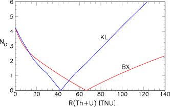
Figure 1 shows the results of our analysis of the total (Th+U) geoneutrino event rate $R$ in KL and BX, in terms of standard deviations ($N_{\sigma}=\sqrt{\Delta\chi^{2}}$) from the best fit. The null hypothesis of vanishing geoneutrino flux ($R=0$) is rejected at $N_{\sigma}\simeq 4.2$ by both KL and BX, in good agreement with the corresponding official results in KL11 and BX10 ; see also Appendix B. Note that the KL and BX curves are not linear and symmetric, as it would be the case for gaussian errors: indeed, the asymmetry and nonlinearity increase for decreasing event rate $R$ (especially for the low-statistics BX data), as a result of Poisson fluctuations, whose statistics is properly accounted for in our $\chi^{2}$ analysis Prev . As a consequence, the current KL and BX event rates cannot be simply summarized in terms of central values and $\pm 1\sigma$ errors: non-gaussian uncertainties must be properly taken into account, in order to exploit the full potential of the available geoneutrino data.

Figure 1: Constraints on the total geoneutrino event rate in KL and BX, in terms of standard deviations $N_{\sigma}$ from the best fit.

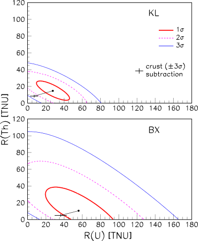
In order not to loose precious information, in the following we shall mostly refer to the full data analysis in terms of separate (not summed) Th and U event rates. Figure 2 shows, in particular, the main results of our analysis of KL and BX data, in the plane charted by the geoneutrino event rates $R(\mathrm{U})$ and $R(\mathrm{Th}$) for KL (upper panel) and BX (lower panel). In both panels, the thick dot represents the best fit, while the curves correspond to the $n\sigma$ contours ($\Delta\chi^{2}=n^{2}$, for $n=1$, 2 and 3), whose projections provide the $n\sigma$ bounds for the corresponding parameter PDGB . Note that, in Fig. 2, the $1\sigma$ contour for KL is closed, i.e., KL can separate the Th and U components at the (weak) level of $\sim 1\sigma$, due to higher statistics and better spectral information. However, already at $2\sigma$, the KL and the BX contours are no longer closed; indeed, the strong anticorrelation of the $n\sigma$ isolines reflects the fact that the KL and BX spectra are currently more sensitive to the total Th+U flux than to their separate Th and U components which, to some extent, can be traded one for the other. Figure 2 also anticipates schematically the subtraction of the estimated crustal rates (with their associated $\pm 3\sigma$ errors), as discussed in detail in the next Sections.

Figure 2: Results of our analysis of geoneutrino rates $R(\mathrm{Th})$ and $R(\mathrm{U})$ expressed in TNU, for both KL (upper panel) and BX (lower panel). The curves represent the $n\sigma$ contours ($\Delta\chi^{2}=n^{2}$) around the best fit (thick dot). Also shown is the shift of the best fit points after subtraction of the estimated crustal components (with their $\pm 3\sigma$ errors). See the text for details.

III Earth science input: Crustal flux estimates in KL and BX

In order to estimate the crustal geoneutrino flux we need a global model for the Earth crust and a sufficiently detailed model for the local contribution. Indeed, due to the inverse square law for the flux, the crust portions within and outside a radius of $O(500)$ km from the detector provide comparable flux contributions in both KL and BX Fi07 . In particular, for both KL and BX, we use an accurate description of the local crust extending over $\sim\!2.5\times 10^{5}$ km² and down to 30–40 km of depth (Moho surface), which contributes to $\sim\!40\%$ of the total geo-$\nu$ signal. For farther portions of the crust, a coarser description in terms of $2^{\circ}\times 2^{\circ}$ tiles is sufficient.

In this section we discuss global and local properties of the crust, building upon previous works on the subject Fi07 ; KLOC ; Colt . In particular, we report our calculation of the crustal Th and U fluxes at KL and BX, with estimated $1\sigma$ uncertainties of O(10%). It should be noted, however, that precise estimates for such uncertainties play no significant role in this work: even if the crustal flux errors were all conservatively doubled or tripled, the final results for the mantle signal would only change by a tiny fraction of one standard deviation (see Appendix A).

III.1 Global model of the crust

Our global model for the crust is based on a geophysical $2^{\circ}\times 2^{\circ}$ tiled map Tile , as well as on the Th and U mass abundances recommended in Sedi for sedimentary layers and in Rudn for the upper, middle, and lower crust. For the lower crust, the values in the literature encompass a large interval: we adopt a mean value together with an uncertainty indicative of the spread of published values Fi07 . After removal of a tiny portion of crust extending for a few hundred km around each site (local or “LOC” contribution, as defined in the next subsections), the global model is used to evaluate the remaining geoneutrino flux at both KL and BX (rest-of-the-crust or “ROC” contribution).

Table I reports the input total mass and adopted values and $\pm 1\sigma$ errors for radiogenic abundances in each global reservoir, as well as the output ROC event rates in KL and BX, multiplied by the central value of the probability in Eq. (5). [The $P_{ee}$ errors are already accounted for in the experimental data fits of Figs. 1 and 2.] Total errors in the last row are obtained by summing partial errors in quadrature.

Table 1: Inputs and outputs of the global model of the crust adopted in this work. The first four columns report, for each reservoir, its mass $M$ and the adopted Th and U mass abundances. The last four columns report the estimated rest-of-the-crust (ROC) event rates, as obtained by excluding from the total crust the local (LOC) portions defined in the text. Quoted errors are at $1\sigma$.

				ROC rates for KL		ROC rates for BX
Reservoir	$M$ [$10^{22}$ kg]	$a$(Th) [$\mu$g/g]	$a$(U) [$\mu$g/g]	$R$(Th) [TNU]	$R$(U) [TNU]	$R$(Th) [TNU]	$R$(U) [TNU]
Sediments	0.11	$6.9\pm 0.8$	$1.7\pm 0.2$	$0.10\pm 0.01$	$0.34\pm 0.04$	$0.22\pm 0.03$	$0.82\pm 0.09$
Upper crust	0.70	$10.5\pm 1.0$	$2.7\pm 0.6$	$0.99\pm 0.10$	$3.64\pm 0.80$	$1.66\pm 0.16$	$6.42\pm 1.43$
Middle crust	0.71	$6.5\pm 0.5$	$1.3\pm 0.4$	$0.62\pm 0.05$	$1.80\pm 0.56$	$1.11\pm 0.09$	$3.32\pm 1.02$
Lower crust	0.66	$3.7\pm 2.4$	$0.6\pm 0.4$	$0.34\pm 0.22$	$0.80\pm 0.54$	$0.59\pm 0.39$	$1.44\pm 0.96$
Oceanic crust	0.60	$0.22\pm 0.07$	$0.10\pm 0.03$	$0.02\pm 0.01$	$0.11\pm 0.04$	$0.01\pm.003$	$0.07\pm 0.02$
Total				$2.07\pm 0.25$	$6.71\pm 1.12$	$3.72\pm 0.43$	$12.07\pm 2.00$

From the global model we estimate the following contributions to the radiogenic crustal heat: $H(\mathrm{Th})=4.02\pm 0.47$ TW and $H(\mathrm{U})=3.40\pm 0.56$ TW. Assuming a mass ratio $\mathrm{K}/\mathrm{U}\sim 13000$ Arev , the additional K contribution would be $H(\mathrm{K})\simeq 1.5\pm 0.2$ TW and the total estimated crustal heat would amount to $H(\mathrm{Th}+\mathrm{U}+\mathrm{K})\simeq 8.9\pm 1.2$ TW, where errors have been added linearly, due to the high positive correlations among the three radiogenic element abundances.

III.2 Local model of the crust around KL

The local crust at the KL site (Kamioka) is defined in terms of six $2^{\circ}\times 2^{\circ}$ tiles, supplemented with geochemical information on a $0.25^{\circ}\times 0.25^{\circ}$ grid and on a detailed map of the crust depth KLOC . The possible effects of the subducting slab beneath Japan are considered, and the uncertainties arising from the debated (continental or oceanic) nature of the crust below the Japan Sea are also taken into account. The maximal and minimal excursions of various inputs and uncertainties are taken as a proxy for the $\pm 3\sigma$ error range.

Table II summarizes the estimated LOC contributions to the geoneutrino signal in KL, together with their estimated $1\sigma$ errors; total errors are obtained by summing in quadrature. Further details can be found in Fi07 ; KLOC .

Table 2: Local (LOC) contributions to the geoneutrino signal in KL. Quoted errors are at $1\sigma$.

Reservoir	$R$(Th) [TNU]	$R$(U) [TNU]
Six tiles	$3.20\pm 0.37$	$11.17\pm 0.65$
Subducting slab	$0.90\pm 0.27$	$2.02\pm 0.61$
Japan sea	$0.09\pm 0.03$	$0.34\pm 0.10$
LOC total	$4.19\pm 0.46$	$13.53\pm 0.90$

III.3 Local model of the crust around BX

The local crust at the BX site (Gran Sasso) is defined in terms of a $2^{\circ}\times 2^{\circ}$ central tile (CT) and of the rest of the region (RR) formed by the surrounding six tiles minus the CT Colt . Geophysical features of the local crust (geometry, density, seismic velocities etc.) are reported in Colt . From a geochemical viewpoint, the CT sedimentary is a mixture of four main reservoirs, which have been probed by direct sampling of Th and U abundances. In the upper and lower crust one can recognize two components (felsic and mafic rocks) which are also probed by direct measurements. Average elemental abundances for the two groups were calculated and seismic arguments used in order to fix their relative amounts within the upper crust. In the lower crust, the fraction of felsic and mafic rocks was estimated on the basis of geophysical and geochemical information. The same Th and U abundances were assumed in the CT and in the RR. The maximal and minimal excursions of various input values and uncertainties were taken as a proxy for the $\pm 3\sigma$ error range.

Table III summarizes the estimated LOC contributions to the geo-$\nu$ signal in BX, together with their $1\sigma$ errors; total errors are obtained by summing in quadrature. Adopted abundances are also reported. See Colt for details.

Table 3: Local (LOC) abundances and contributions to the geoneutrino signal in BX. Quoted errors are at $1\sigma$.

Reservoir	$a(\mathrm{Th})$ [$\mu$g/g]	$a(\mathrm{U})$ [$\mu$g/g]	$R$(Th) [TNU]	$R$(U) [TNU]
Sediments	$2.00\pm 0.17$	$0.80\pm 0.07$	$0.40\pm 0.04$	$2.53\pm 0.21$
Upper crust	$8.1\pm 1.6$	$2.20\pm 0.43$	$1.21\pm 0.24$	$4.94\pm 0.96$
Lower crust	$2.6\pm 1.2$	$0.30\pm 0.10$	$0.25\pm 0.11$	$0.34\pm 0.11$
LOC total			$1.86\pm 0.27$	$7.81\pm 0.99$

III.4 Estimated crustal geoneutrino rates and uncertainties at KL and BX

Table IV summarizes the results of this section, in terms of LOC, ROC and total event rates in KL and BX, with errors added in quadrature. The fractional uncertainties, all of $O(10\%)$, are not crucial in the context of our analysis, which is dominated by experimental errors (see below and Appendix A). In the future, however, it might be useful to address some geophysical uncertainties—such as those related to the global crust thickness—which have been neglected herein, in comparison with the larger geochemical abundance uncertainties.

Concerning the central values, it should be noted that the total estimated rates in BX are lower than in KL, contrary to previous estimates and expectations (based on the fact that BX is surrounded by thicker crust than KL) Fi07 ; Hawa . This counterintuitive result is mainly driven by the improved description of the local BX crust performed in Colt , leading to a significantly deeper sediment layer, and to a depletion of Th and U in all local crust reservoirs, as compared to previous estimates using no (or less accurate) local models.

Table 4: Summary of LOC, ROC and total crust contributions to the geo-$\nu$ signal in KL and BX. Quoted errors are at $1\sigma$.

	KL event rates		BX event rates
Reservoir	$R$(Th) [TNU]	$R$(U) [TNU]	$R$(Th) [TNU]	$R$(U) [TNU]
LOC	$4.19\pm 0.46$	$13.53\pm 0.90$	$1.86\pm 0.27$	$7.81\pm 0.99$
ROC	$2.07\pm 0.25$	$6.71\pm 1.12$	$3.60\pm 0.43$	$12.07\pm 2.00$
Crust total	$6.26\pm 0.52$	$20.24\pm 1.43$	$5.46\pm 0.51$	$19.88\pm 2.24$

IV Crust subtraction and geoneutrino rates from the mantle

In the previous two sections we have determined, for both KL and BX, the experimental total rates $R$ (Fig. 1) and the theoretical crustal rates $R_{\mathrm{crust}}$ (Table IV) due to Th and U geoneutrinos, together with the associated uncertainties. In this section we infer the mantle rates, by subtracting the estimated crustal components from the experimental total rates,

$$R(\mathrm{mantle})=R(\mathrm{total,\ exp})-R(\mathrm{crust,\ theo})\ .$$ (6)

Going back to Fig. 2, in each panel, crustal rate subtraction is graphically shown as a shift of the best-fit point by a vector (ending with crossed error bars) defined by the total Th and U crust rates and their $\pm 3\sigma$ errors (see Table IV). In principle, such estimated crust uncertainties should be properly combined with the experimental rate uncertainties. However, the latter are currently larger by (more than) an order of magnitude, and dominate the error associated to the subtraction procedure. Indeed, in Appendix A we demonstrate that, in the present context, crustal rate errors are practically insignificant, even if they are conservatively inflated by a factor of a few. As a consequence, the $n\sigma$ contours for the mantle rates can be simply obtained by rigidly shifting the $n\sigma$ contours in Fig. 1, together with the best fit point, along the slanted line. Numerically, this amounts to a simple translation of the two-dimensional $\chi^{2}$ functions for both KL and BX.

Figure 3: Mantle geoneutrino rates obtained from crustal rate subtraction in KL (upper panel) and BX (middle panel), as well as in their combination KL+BX (lower panel). The curves represent the $n\sigma$ contours around the best fit. In the lower panel, lines of constant Th/U abundance ratio are also shown. The null hypothesis (no mantle signal) is disfavored at $>2\sigma$ by KL+BX.

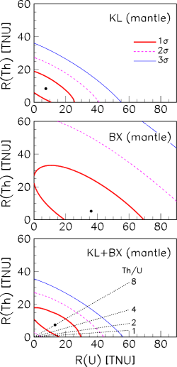
Figure 3 shows the allowed $n\sigma$ regions of the mantle rates resulting from crust subtraction in KL (upper panel) and in BX (middle panel). In both cases, positive values for the Th and U mantle rates are preferred. The fact that the best fit rates are well within the physical region (and none of them is negative) is an encouraging sanity check of the crust subtraction procedure. More precisely, we find that the null hypothesis of no mantle signal (i.e., the origin of the axes) is disfavored at about $1.7\sigma$ level in KL and $2.0\sigma$ in BX. Moreover, the allowed regions in KL and BX largely overlap. Therefore, we have obtained two consistent hints at $\geq 1.7\sigma$ level in favor of a geoneutrino signal coming from the mantle. Nonzero mantle fluxes were also suggested (but not quantified) by the analyses in KL11 ; Prev .

The above hints can now be properly combined under the assumption of site-independent mantle flux, which is justified in the absence of significant indications in favor of local mantle anomalies below the KL or BX sites. (Possible geochemical mantle anomalies are still debated and, in any case, they are strongly model dependent Anom .) Under such hypothesis, the combination of KL and BX constraints on mantle geoneutrino rates amount to summing the corresponding $\chi^{2}$ functions. The results are shown in the lower panel of Fig. 3. The mantle signal common to the KL and BX emerges now with greater statistical significance, the null hypothesis being rejected at $2.4\sigma$ (about $98.4\%$ C.L.). This result represents an encouraging first step towards a better understanding of the mantle via geoneutrinos, and can already provide valuable indications in comparison with various mantle models, as shown in the next Section.

Of course, the inferred mantle signal is not yet accurate enough to probe more detailed issues, such as the mantle Th/U ratio. In particular, in Fig. 3, the KL+BX contour at $1\sigma$ appears to be compatible with any possible Th/U mantle ratio (some isolines being shown to guide the eye), so that the preference for Th/U $\simeq 8$ is not statistically significant. A future reduction of the experimental errors (which is conceivable with longer exposures, better background rejection, and additional experiments) would be desirable to get a mantle geoneutrino signal with greater impact for geophysics and geochemistry.

V Comparison with mantle models

In this Section we compare the inferred mantle geoneutrino signal with predictions derived from various published mantle models, hereafter referred to as: Turcotte and Schubert 2002 Turc , Anderson 2007 Ande , Palme & O’Neill 2003 Palm , Allegre et al. 1995 Alle , McDonough & Sun 1995 McDo , Lyubetskaya & Korenaga 2007 Lyub , Javoy et al. 2010 Javo . It should be remarked that, in general, the models mainly focus on the “primitive mantle” (PM, with mass $M_{\mathrm{PM}}=4.03\times 10^{24}$ kg) prior to differentiation into crust and “present mantle,” while our results correspond, of course, only to the present mantle. Therefore, in order to perform a comparison with the results obtained in the previous Section, for each model we remove from the PM the crustal Th and U masses (which, in our global crust model of Sec. III, amount to $M_{\mathrm{Th}}=15.30\pm 1.77$ and $M_{\mathrm{U}}=3.45\pm 0.57$ at $1\sigma$, in units of $10^{16}$ kg).

The distribution of the remainder Th and U masses within the present mantle volume is subject to a lively debate, opposing homogeneous versus inhomogeneous (e.g., layered) models Fi07 ; Mc08 . For the purposes of this work, we consider two representative extreme scenarios, yielding “high” and “low” mantle geoneutrino rates. The “high rate” (homogeneous) scenario is obtained by subtraction of the Th and U crustal masses at the lower end of their $1\sigma$ range, and distributing the remainder in the whole mantle at constant density. The “low rate”(inhomogeneous) scenario is obtained by subtracting from the PM the Th and U crustal masses at the upper end of their $1\sigma$ range, and placing all the remainder in the so-called D” layer (250 km thickness) just above the core-mantle boundary. In both cases, averaged oscillations are included. Note that the various models are based on different assumptions or input values about the primitive chondritic material, which lead to further differences in the Th and U contents and in the associated radiogenic heat in the present mantle.

Table V summarizes our estimated “low” and “high” Th and U mantle geoneutrino rates as derived from each mantle model, together with the associated total heat $H(\mathrm{Th}+\mathrm{U})$. Note that two models (Allegre et al. 1995, McDonough & Sun 1995) are practically identical for our purposes. In one model (Javoy et al. 2010), characterized by rather low radiogenic abundances, the Th content of the PM is slightly lower than the corresponding content of the crust in our “low” scenario; crustal subtraction would then yield slightly negative results, which have been just set to zero. Since not all models in Table V are endowed with PM error estimates, we do not quote individual errors for the present mantle rates; their spread is, however, indicative of the large theoretical uncertainties typically associated to mantle observables.

Table 5: Geoneutrino event rates derived from various models of the primitive mantle (PM), under different assumptions about the Th and U distributions in the present mantle, leading to “low” and “high” rates. The first three columns characterize the original PM model in terms of Th and U masses. After crustal subtraction and redistribution of the remaining Th and U masses in the present mantle, we derive the oscillated Th and U mantle event rates, the Th+U heat and the Th/U ratio as reported in the last eight columns, for the “low” and “high” scenarios.

Primitive mantle characteristics			Present mantle, “low” scenario				Present mantle, “high” scenario
Model	$M_{\mathrm{Th}}$	$M_{\mathrm{U}}$	$R(\mathrm{Th})$	$R(\mathrm{U})$	$H(\mathrm{Th+U})$	Th/U	$R(\mathrm{Th})$	$R(\mathrm{U})$	$H(\mathrm{Th+U})$	Th/U
	[$10^{17}$kg]	[$10^{17}$kg]	[TNU]	[TNU]	[TW]		[TNU]	[TNU]	[TW]
Turcotte & Schubert 2002	3.62	0.90	2.7	9.8	17.0	3.9	3.9	14.7	19.0	3.8
Anderson 2007	3.13	0.78	2.3	8.4	14.5	3.9	3.4	12.8	16.6	3.8
Palme & O’Neil 2003	2.06	0.54	1.3	5.7	9.1	3.4	2.1	9.2	11.2	3.4
Allegre et al. 1995	1.80	0.46	1.1	4.7	7.7	3.6	1.9	8.0	9.8	3.5
McDonough & Sun 1995	1.80	0.46	1.1	4.7	7.7	3.6	1.9	8.0	9.8	3.5
Lyubetskaya & Korenaga 2007	1.26	0.34	0.7	3.3	5.0	2.0	1.2	6.0	7.0	3.0
Javoy et al. 2010	0.48	0.14	0.0	1.0	0.8	0.0	0.4	3.0	2.8	1.7

Figure 4: Comparison of experimental constraints and model predictions in the plane charted by the Th and U mantle rates. Each model leads to extremal case of “low” and “high” rates, connected by lines to guide the eye. The KL+BX constraints are shown as $n\sigma$ contours in steps of $0.5\sigma$. See the text for details.

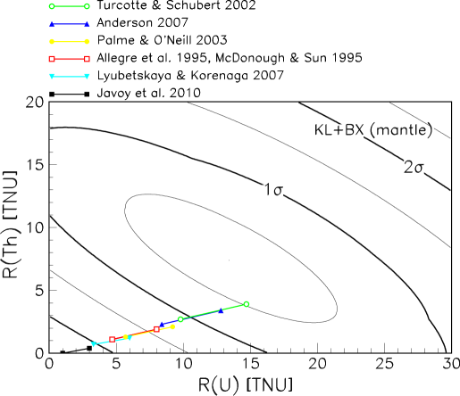
Figure 4 shows the same KL+BX mantle rate constraints as in the lower panel of Fig. 3, but with superimposed model predictions from Table V. In order to guide the eye, the “low” and “high” predictions for each model are connected by a straight line; moreover, the KL+BX $n\sigma$ isolines are shown in steps of $0.5\sigma$. It appears that the data prefer mantle models with relatively high radiogenic contents (e.g., Turcotte & Schubert 2002) and disfavor at $\sim 2\sigma$ those with low contents (e.g., Javoy et al. 2010). This indication is rather interesting and deserves to be checked and investigated with further data, given its potential impact on mantle model building.

The near alignment of all model predictions in Fig. 4 reflects the narrowness of the Th/U mantle ratio in Table V, $\mathrm{Th/U}\in[1.7,\,3.9]$. In this context, it makes sense to marginalize away the Th/U ratio within such range, and to express the resulting rates in terms of the total (Th+U) event rate. We find at $1\sigma$ that

$$R(\mathrm{Th+U,\ mantle})\simeq 23\pm 10~{}\mathrm{TNU}\ (\mathrm{KL+BX},\mathrm{for\ Th/U}\in[1.7,\,3.9])\ ,$$ (7)

with nearly gaussian error distribution (not shown). At present, this represents our best estimate for the mantle geoneutrino flux, as derived by using inputs from particle physics (KL, BX, and oscillation data) and from Earth sciences (crustal data and mantle Th/U ratio).

Finally, Fig. 5 shows a comparison between theory and data in terms of the Th+U mantle rate (in TNU) and radiogenic heat (in TW). The various model predictions, shown as lines connecting the “low” and “high” cases in Table V, can be compared to the mantle rate inferred in Eq. (7) and shown as a horizontal $1\sigma$ band. Notice that the $1\sigma$ experimental error is already comparable to the spread of the theoretical rate predictions: therefore, improvements in the experimental accuracy by a factor of two or more, would allow a statistically significant model discrimination. At present we note that, at $1\sigma$, the data favor models with relatively high mantle heat $H(\mathrm{Th+U})$, such as Anderson 2007 and Turcotte & Schubert 2002. However, no model can be really excluded at $\sim 2\sigma$.

Figure 5: Comparison of KL+BX constraints ($1\sigma$ horizontal band) and model predictions (slanted lines) in the plane charted by the Th+U geoneutrino rate and radiogenic heat for the mantle.

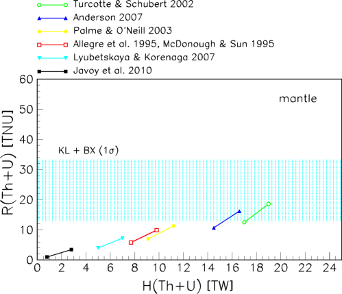
Signal-heat correlation plots as in Fig. 5 have been suggested earlier Fi07 as a way to constrain the radiogenic heat, whose preferred range should be determined by the intersection of the slanted “theoretical” band (i.e., the envelope of all models) with the horizontal “experimental” band. At present, given the large uncertainties affecting the bands in Fig. 5, we refrain from deriving a preferred range for the mantle heat—a task which is left to future studies involving more accurate data and, possibly, more extensive model surveys. We just observe that Fig. 5 suggests a lower bound for the Th+U mantle heat, which appears to exceed $\sim 13$ TW at $1\sigma$; then, adding no less than $\sim 6$ TW from Th+U crustal heat (see Sec. III A), we infer a tentative lower bound of $\sim 19$ TW (at $1\sigma$) for the total Th+U radiogenic heat in the Earth, compatible with the estimate $\sim 20\pm 9$ TW of KL11 .

VI Summary and conclusions

In this work, we have analyzed in detail the experimental total rates of Th and U geoneutrino events in KamLAND (KL) and Borexino (BX), including neutrino oscillation effects. We have calculated the crustal flux at the two detector sites, using updated information about the global and local Th and U distribution. After subtraction of the estimated crustal component from the total fluxes, we find hints for residual mantle components at $\gtrsim 1.5\sigma$ in both KL and BX. In the KL+BX combination, the statistical significance of the mantle signal reaches the $2.3\sigma$ level. In particular, for typical Th/U mantle ratios, we estimate a total mantle rate of $R(\mathrm{Th}+\mathrm{U})\simeq 23\pm 10$ TNU (including oscillation effects). The $\pm 10$ TNU error is comparable to the spread of rate predictions derived from various published models of the mantle. Among these, a preference is found for models with relatively high radiogenic contents (corresponding to present mantle Th+U heat $\gtrsim 13$ TW at $\sim 1\sigma$). However, no model can be excluded at $\gtrsim 2\sigma$ level yet.

The accuracy of the results can be improved in part by further KL and BX data, and especially by prospective data from future experiments at different sites. If Th and U rates from several different detectors were available, one could estimate and subtract the crust components in all of them, in order to infer the corresponding mantle components. Should all mantle rates be the same within errors, the hypothesis of a common, isotropic mantle geoneutrino flux would be corroborated, and its value could be obtained by combining the results from all the experiments. Conversely, one should consider the possibility of an anisotropic mantle flux, or of incorrect estimates of (some of) the subtracted crustal fluxes. Mantle-dominated measurements at oceanic sites would provide crucial tests of the various options and additional constraints for mantle models. In any case, we shall learn a lot more about the Earth mantle from future geoneutrino data, supplemented by detailed descriptions of the crust at global and local scales, in a truly interdisciplinary approach.

Appendix A Central values and uncertainties of estimated crustal rates

In this work, a careful evaluation of crustal geoneutrino rates has been carried out (Sec. III) in order to infer the mantle signal by subtraction (Sec. IV). In this Appendix, we discuss possible effects or additional constraints that might slightly change either the central values or the uncertainties of our estimated crustal fluxes; we argue that such changes are not expected to significantly weaken the inferred mantle signal.

A.1 Central values

In Sec. III, crustal rates have been estimated by summing the LOC (local) component, based on a detailed description of the crust near the detector site, and the ROC (rest-of-the-crust) component, based on state-of-the-art information about the global structure and radiogenic contents of the crust.

Of course, the global model of the crust used in Sec. III can be improved by adding new data or constraints, which might also lead to variations in the central ROC values. In particular, heat-flow measurements at local, regional, and global scales appear to provide particularly promising and independent constraints Mare . In this context, we note that a recent heat-flow evaluation of the total radiogenic heat of the crust suggests a value $H(\mathrm{Th}+\mathrm{U}+\mathrm{K})\simeq 7.5\pm 0.7$ TW Heat (as quoted in Mare ), which is $\sim 20\%$ lower than our estimate $8.9\pm 1.2$ TW in Sec. III, although compatible within the quoted $1\sigma$ errors. At present, it is not obvious if and how the above heat-flow estimate should be added as an additional input; in any case, its possible inclusion would presumably lead to an $O(10\%)$ decrease of the adopted global Th and U crust abundances, and to an associated decrease of the estimated ROC fluxes in both KL and BX. The mantle flux estimated by subtraction would then slightly increase, and the hints for a mantle signal discussed in Sec IV would be strenghtened.

Another issue concerns the approximation of averaged oscillations. While this approximation is certainly justified for the ROC component, it may be slightly inaccurate for the LOC component. We have re-calculated the LOC rates for the unaveraged oscillation probability in Eq. (3), and we find the following fractional variations with respect to the LOC rates in Table IV: $+1\%$ (Th) and $+3\%$ (U) for KL, and $-7\%$ and $-6\%$ for BX. [In BX, a larger fraction of local flux is suppressed by the first dip of the oscillation probability.] In terms of total (ROC+LOC) rates, all such variations are smaller than $\pm 2.5\%$ and can be ignored in practice (see also below). Note that, if the effects of unaveraged oscillations were statistically relevant for LOC estimates, then the analysis of geoneutrino energy spectra should also account for small $L/E$ effects (not included in the present work).

Based on the above considerations and on our educated guess, we surmise that future improvements in the local and global description of the crust are unlikely to change our estimated crustal rates by much more than $O(10\%)$, which is also the size of the uncertainties in Table IV. Uncertainties of this (and even twice as large) size are negligible in the context of the present work, as we demonstrate below.

A.2 Uncertainties

In Sec IV we have inferred the mantle geoneutrino rates by subtracting the crust component from the total experimental rates, whose errors have been claimed to dominate the results. The irrelevance of the theoretical crust rate errors can be easily demonstrated in the case of KL, where the $n\sigma$ experimental contours in the upper panel of Fig. 2 are nearly elliptical and equally spaced (i.e., the correlated errors can be approximated by a bivariate gaussian).

In order to simplify the argument and the notation, let us call $(x,\,y)$ the total KL experimental U and Th rates shown in the upper panel of Fig. 2, in TNU units. The allowed contours are well approximated by ellipses centered at $(27.8,\,14.5)$ and with $1\sigma$ error matrix

$$\bm{\sigma}^{2}=\left(\begin{array}[]{cc}\sigma^{2}_{x}&\rho\,\sigma_{x}\sigma_{y}\\ \rho\sigma_{x}\sigma_{y}&\sigma^{2}_{y}\end{array}\right)\ ,$$ (8)

where $\sigma_{x}=18.6$, $\sigma_{y}=11.4$, and $\rho=-0.75$. If we simply subtract the crustal rates $(x_{c},\,y_{c})\simeq(20.2,\,6.3)$ in Table IV with no errors, we get an estimated mantle signal $(x_{m},\,y_{m})=(7.6,\,8.2)$, with the same error matrix as above. The corresponding $\chi^{2}$ function PDGB equals $2.57\simeq 1.6^{2}$ at the point $(0,\,0)$, namely, the null hypothesis of “no mantle signal” is rejected at $1.6\sigma$ in this gaussian approximation for the KL experimental errors (consistently with the non-approximated value of $1.7\sigma$ reported in Sec. IV).

If the KL crustal rate errors in Table III are included with a (presumably positive) correlation $\rho_{c}$ in a crust error matrix $\bm{\sigma}_{c}$, the mantle error matrix is augmented as $\bm{\sigma}^{2}_{m}=\bm{\sigma}^{2}+\bm{\sigma}^{2}_{c}$. The null hypothesis is then rejected at $1.58$–$1.59\sigma$, depending on $\rho\in[0,\,1]$. Therefore, the inclusion of crustal rate errors changes the statistical significance of the mantle signal in KL by a negligible fraction of one standard deviation ($0.02\sigma$ or less). If we repeat the above exercise with crustal errors doubled (or tripled) for the sake of conservativeness, then the significance of the mantle signal in KL is lowered by less than $0.08\sigma$ (or $0.18\sigma$). For BX (middle panel of Fig. 3), the effect of crustal errors can only be smaller, since the experimental errors are significantly larger than in KL. Therefore, we surmise that the $2.4\sigma$ statistical significance of the mantle signal (Sec. IV) could be lowered by about 0.1–$0.2\sigma$ in the worst cases.

Summarizing, variations or uncertainties of the estimated crustal rates at the level of $O(10\%)$ can be practically ignored in the context of this work, whose results are dominated by the—much larger—experimental errors on geoneutrino event rates. In the future, when theoretical and experimental errors will be comparable, a proper convolution of their distributions will be required in order to obtain reliable error estimates for the inferred mantle geoneutrino rate.

Appendix B Side results of the KL and BX data analysis

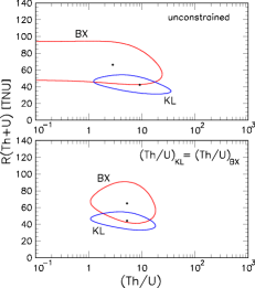
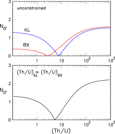
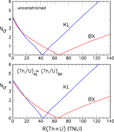
In this Appendix we supplement the data analysis reported in Sec. II and in Fig. 1 with additional results, concerning total rates only, with no separation between mantle and crust components. As in Prev , we re-express the experimental constraints in terms of total Th+U rates and Th/U abundance ratios, instead of separate Th and U geoneutrino rates. This alternative formulation is particularly useful to evaluate the effects of assuming, in first approximation, the same average Th/U ratio in both KL and BX Prev . The results are shown in the various panels of Fig. 5.

Figure 6(a) shows the best fits and $1\sigma$ contours in the plane charted by the total rate $R(\mathrm{Th}+\mathrm{U})$ and by the average Th/U abundance ratio. In the upper panel, these observables are left free for both KL and BX. Both experiments provide similar (although weak) upper bounds on Th/U, but only KL sets a lower limit at present, $\mathrm{Th}/\mathrm{U}\gtrsim 1$. In the lower panel, under the assumption of a common Th/U ratio in KL and BX, we obtain a best fit $\mathrm{Th}/\mathrm{U}\simeq 5$, close to the typical chondritic value $\mathrm{Th}/\mathrm{U}\simeq 3.9$ Rati , although with very large uncertainties (a factor of about four).

Figure 6(b) shows the constraints on the Th/U abundance ratio in terms of standard deviations $N_{\sigma}$ (the total rate being marginalized away). As in Fig. 6(a), the upper panel refers to the unconstrained fit, while the lower panel refers to the case with the same Th/U in KL and BX. It can be seen that, in combination, KL+BX can set for the first time a $2\sigma$ upper bound on Th/U, although it is still very weak ($\mathrm{Th}/\mathrm{U}\lesssim 10^{2}$). In this context, significant progress will require geoneutrino energy spectra with high statistics and low systematics, in order to better discriminate the different Th and U components and to constrain their ratio with higher accuracy.

Finally, Fig. 6(c) shows the constraints on the total rate $R(\mathrm{Th}+\mathrm{U})$ in terms of standard deviations $N_{\sigma}$ (the Th/U ratio being marginalized away). The upper panel coincides with Fig. 1. The lower panel is rather similar, implying that current constraints on the total Th+U rate are not very sensitive to specific assumptions on the Th/U ratio.

(a)  Best fits and $1\sigma$ contours in the plane of the Th+U rate versus the Th/U ratio.

(b)  Constraints on the Th/U ratio in terms of standard deviations $N_{\sigma}$ from the best fit.

(c)  Constraints on the Th+U rate in terms of standard deviations $N_{\sigma}$ from the best fit.

Figure 6: Analysis of KL and BX data in terms of the total Th+U event rate and of the average Th/U abundance ratio. In all the subfigures, the lower (upper) panel does (not) include the assumption of equal Th/U in KL and BX.

References

- (1) G. Fiorentini, M. Lissia and F. Mantovani, “Geo-neutrinos and Earth’s interior,” Phys. Rept. 453, 117 (2007).
- (2) KamLAND Collaboration, A. Gando et al., “Partial radiogenic heat model for Earth revealed by geoneutrino measurements,” Nature Geoscience 4, 647 (2011). First KamLAND results were reported in T. Araki et al., “Experimental investigation of geologically produced antineutrinos with KamLAND,” Nature 436, 499 (2005).
- (3) Borexino Collaboration, G. Bellini et al., “Observation of Geo-Neutrinos,” Phys. Lett. B 687, 299 (2010).
- (4) W.F. McDonough and R. Arevalo Jr., “Uncertainties in the composition of Earth, its core and silicate sphere,” Proceedings on Neutrino 2008, XXIII International Conference on Neutrino Physics and Astrophysics (Christchurch, New Zealand, 2008), ed. by J. Adams, F. Halzen, and S. Parke, Journal of Physics Conference Series 136, 022006 (2008).
- (5) J.-C. Mareschal, C. Jaupart, C. Phaneuf and C. Perry, “Geoneutrinos and the energy budget of the Earth,” Journal of Geodynamics 54, 43 (2012).
- (6) S. Dye (Editor), “Neutrino Geophysics,” Proceedings of Neutrino Sciences 2005 (Honolulu, Hawaii, 2005), Earth, Moon, and Planets 99 (2006), 368 pp.
- (7) M. Batygov, “On the possibility of directional analysis for geoneutrinos,” in “Neutrino Geophysics” Hawa , p. 183.
- (8) B.D. Fields and K.A. Hochmuth, “Imaging the Earth’s interior: The angular distribution of terrestrial neutrinos” Hawa , p. 155.
- (9) S. T. Dye, “Geo-neutrinos and Silicate Earth Enrichment of U and Th,” Earth Planet. Sci. Lett. 297, 1 (2010).
- (10) G.L. Fogli, E. Lisi, A. Palazzo, and A.M. Rotunno, “Geoneutrinos: A systematic approach to uncertainties and correlations,” in “Neutrino Geophysics” Hawa , p. 111.
- (11) J. Blichert-Toft, B. Zanda, D.S. Ebel and F. Albarède, “The Solar System primordial lead,” Earth Planet. Sci. Lett. 300, 152 (2010).
- (12) G.L. Fogli, E. Lisi, A. Palazzo and A.M. Rotunno, “Combined analysis of KamLAND and Borexino neutrino signals from Th and U decays in the Earth’s interior,” Phys. Rev. D 82, 093006 (2010).
- (13) G. L. Fogli, E. Lisi, A. Marrone, A. Palazzo and A. M. Rotunno, “Evidence of from global neutrino data analysis,” Phys. Rev. D 84, 053007 (2011).
- (14) F. P. An et al. [Daya Bay Collaboration], “Observation of electron-antineutrino disappearance at Daya Bay,” arXiv:1203.1669 [hep-ex].
- (15) S.-B. Kim et al. [RENO Collaboration], “Observation of Reactor Electron Antineutrino Disappearance in the RENO Experiment,” arXiv:1204.0626 [hep-ex].
- (16) J. Beringer et al. (Particle Data Group), Phys. Rev. D 86, 010001 (2012).
- (17) G. L. Fogli, E. Lisi, A. Marrone, D. Montanino, A. Palazzo and A. M. Rotunno, “Global analysis of neutrino masses, mixings and phases: entering the era of leptonic CP violation searches,” arXiv:1205.5254 [hep-ph], to appear in Phys. Rev. D.
- (18) G. Fiorentini, M. Lissia, F. Mantovani and R. Vannucci, “How much Uranium is in the Earth? Predictions for geo-neutrinos at KamLAND,” Phys. Rev. D 72, 033017 (2005).
- (19) M. Coltorti et al., “U and Th content in the Central Apennines continental crust: A contribution to the determination of the geo-neutrinos flux at LNGS,” Geochimica et Cosmochimica Acta 75, 2271 (2011).
- (20) G. Laske, G. Masters and C. Reif, “CRUST 2.0: A New Global Crustal Model at Degrees,” available at the website: igppweb.ucsd.edu/∼gabi/rem.html.
- (21) T. Plank and C. Langmuir, “The chemical composition of subducting sediment and its consequences for the crust and mantle,” Chem. Geol. 145, 325 (1998).
- (22) R.L. Rudnick and S. Gao, “The Composition of the Continental Crust,” in Treatise on Geochemistry, ed. by H.D. Holland and K.K. Turekian (Elsevier-Pergamon, Oxford, 2003), vol. 3, p. 1.
- (23) R. Arevalo Jr, W.F. McDonough, and M. Luong, “The K/U ratio of the silicate Earth: Insights into mantle composition, structure and thermal evolution,” Earth Planet. Sci. Lett. 278, 361 (2009).
- (24) W.F. McDonough, talk at the SNOLAB Grand Opening Workshop (Sudbury, Ontario, Canada, 2012), available at www.snolab.ca; and poster at the same Workshop, by O. Sramek, W.F. McDonough, E.S. Kite, V. Levic, S.T. Dye, and S. Zhong, “Geoneutrino flux from Earth’s mantle and its detectability.”
- (25) D. Turcotte and G. Schubert, Geodynamics (Cambridge University Press, NY, 2002), 472 pp.
- (26) D.L. Anderson, New Theory of the Earth (Cambridge University Press, NY, 2007), 400 pp.
- (27) H. Palme and H.S. O’Neill, “Composition of the Primitive Mantle,” in Treatise on Geochemistry Rudn , vol. 2, p. 1.
- (28) C.J. Allegre, J.-P. Poirier, E. Humler and A.H. Hofmann, “The chemical composition of the Earth,” Earth Planet. Sci. Lett. 134, 515 (1995).
- (29) W.F. McDonough and S. Sun, “The composition of the Earth,” Chemical Geology 120, 223 (1995).
- (30) T. Lyubetskaya and J. Korenaga, “Chemical composition of Earth s primitive mantle and its variance: 1. Method and results,” J. Geophys. Res. 112, B03211 (2007).
- (31) M. Javoy et al., “The chemical composition of the Earth: Enstatite chondrite models,” Earth Planet. Sci. Lett. 293, 259 (2010).
- (32) C. Jaupart and J.-C. Mareschal, “Constraints on Crustal Heat Production from Heat Flow Data” in Treatise on Geochemistry Rudn , vol. 3, p. 65.