Estimating the Upcrossings Index

J.R. Sebastião 111 Escola Superior de Gestão, Instituto Politécnico de Castelo Branco, 6000 Castelo Branco, Portugal.
E-mail:jrenato@esg.ipcb.pt

Escola Superior de Gestão
Instituto Politécnico de Castelo Branco
Portugal
   A.P. Martins, H. Ferreira, L. Pereira 222Departamento de Matemática, Universidade da Beira Interior, 6200 Covilhã, Portugal. E-mail:amartins@mat.ubi.pt; lpereira@mat.ubi.pt; helena@mat.ubi.pt
Departamento de Matemática
Universidade da Beira Interior
Portugal

Abstract: For stationary sequences, under general local and asymptotic dependence restrictions, any limiting point process for time normalized upcrossings of high levels is a compound Poisson process, i.e., there is a clustering of high upcrossings, where the underlying Poisson points represent cluster positions, and the multiplicities correspond to cluster sizes. For such classes of stationary sequences there exists the upcrossings index η,𝜂\eta, 0η1,0𝜂10\leq\eta\leq 1, which is directly related to the extremal index θ,𝜃\theta, 0θ1,0𝜃10\leq\theta\leq 1, for suitable high levels. In this paper we consider the problem of estimating the upcrossings index η𝜂\eta for a class of stationary sequences satisfying a mild oscillation restriction. For the proposed estimator, properties such as consistency and asymptotic normality are studied. Finally, the performance of the estimator is assessed through simulation studies for autoregressive processes and case studies in the fields of environment and finance.

Keywords: Upcrossings index, local dependence conditions, consistency and asymptotic normality.

Mathematics Subject Classification (2000) 60G70

1 Introduction and preliminary results

Let 𝐗={Xn}n1𝐗subscriptsubscript𝑋𝑛𝑛1{\bf{X}}=\{X_{n}\}_{n\geq 1} be a stationary sequence and 𝐮={un}n1𝐮subscriptsubscript𝑢𝑛𝑛1{\bf{u}}=\{u_{n}\}_{n\geq 1} a sequence of real levels. We say that 𝐗𝐗\bf{X} has an upcrossing of unsubscript𝑢𝑛u_{n}, at i𝑖i, if the event {Xiun<Xi+1},subscript𝑋𝑖subscript𝑢𝑛subscript𝑋𝑖1\{X_{i}\leq u_{n}<X_{i+1}\}, i=1,,n,𝑖1𝑛i=1,\ldots,n, occurs. The point process of upcrossings of unsubscript𝑢𝑛u_{n} by the first n𝑛n variables of 𝐗𝐗{\bf{X}} is then defined by

N~n(B)=i=1n11I{Xiun<Xi+1}δin(B),B[0,1],n1,formulae-sequencesubscript~𝑁𝑛𝐵superscriptsubscript𝑖1𝑛11subscriptIsubscript𝑋𝑖subscript𝑢𝑛subscript𝑋𝑖1subscript𝛿𝑖𝑛𝐵formulae-sequence𝐵01𝑛1\widetilde{N}_{n}(B)=\sum_{i=1}^{n-1}{1\kern-1.99997pt\rm I}_{\{X_{i}\leq u_{n}<X_{i+1}\}}\delta_{\frac{i}{n}}(B),\qquad B\subset[0,1],\ n\geq 1, (1.1)

where δa()subscript𝛿𝑎\delta_{a}(\cdot) denotes unit mass at aB𝑎𝐵a\in B measure and 1IA1subscriptI𝐴{1\kern-1.99997pt\rm I}_{A} the indicator of event A𝐴A.

Ferreira [4] showed that if 𝐗𝐗{\bf{X}} satisfies the mixing Δ(𝐮)Δ𝐮\Delta({\bf{u}}) condition, introduced in Hsing et al. [9], and N~nsubscript~𝑁𝑛\widetilde{N}_{n} converges in distribution (as a point process on [0,1]), then the limit is necessarily a compound Poisson process. For independent and identically distributed (i.i.d.) sequences it is easy to see that N~nsubscript~𝑁𝑛\widetilde{N}_{n} converges in distribution if and only if unun(ν)subscript𝑢𝑛superscriptsubscript𝑢𝑛𝜈u_{n}\equiv u_{n}^{(\nu)} for some ν>0,𝜈0\nu>0, where un(ν)superscriptsubscript𝑢𝑛𝜈u_{n}^{(\nu)} are normalized levels for upcrossings, that is, 𝐮(ν)={un(ν)}n1superscript𝐮𝜈subscriptsuperscriptsubscript𝑢𝑛𝜈𝑛1{\bf{u}}^{(\nu)}=\{u_{n}^{(\nu)}\}_{n\geq 1} denotes a sequence that satisfies

limn+nP(X1un(ν)<X2)=ν,subscript𝑛𝑛𝑃subscript𝑋1superscriptsubscript𝑢𝑛𝜈subscript𝑋2𝜈\lim_{n\to+\infty}nP(X_{1}\leq u_{n}^{(\nu)}<X_{2})=\nu, (1.2)

being the limit point process a Poisson process on [0,1] with intensity ν.𝜈\nu. We remark that when 𝐗𝐗{\bf{X}} is a stationary sequence, satisfying the long range dependence condition D(𝐮(ν))𝐷superscript𝐮𝜈D({\bf{u}}^{(\nu)}) of Leadbetter [12] and the mild oscillation restriction D′′(𝐮(ν))superscript𝐷′′superscript𝐮𝜈D^{\prime\prime}({\bf{u}}^{(\nu)}) of Leadbetter and Nandagopalan [13], N~nsubscript~𝑁𝑛\widetilde{N}_{n} converges in distribution to the same Poisson process as in the i.i.d. case (Leadbetter and Nandagopalan [13]). When 𝐗𝐗{\bf{X}} only satisfies condition Δ(𝐮(ν))Δsuperscript𝐮𝜈\Delta({\bf{u}}^{(\nu)}) the limit compound Poisson process N~~𝑁\widetilde{N} is in fact a direct consequence of the clustering of high level upcrossings in a dependent sequence. Its intensity is simply ην,𝜂𝜈\eta\nu, where η𝜂\eta is the upcrossings index, and has multiplicity distribution π~(j)=limn+π~n(j),~𝜋𝑗subscript𝑛subscript~𝜋𝑛𝑗\widetilde{\pi}(j)=\lim_{n\to+\infty}\widetilde{\pi}_{n}(j), j=1,2,,𝑗12j=1,2,\ldots, with

π~n(j)=P(i=1rn1I{Xiun<Xi+1}=j|i=1rn1I{Xiun<Xi+1}>0),j=1,2,\widetilde{\pi}_{n}(j)=P\left(\sum_{i=1}^{r_{n}}{1\kern-1.99997pt\rm I}_{\{X_{i}\leq u_{n}<X_{i+1}\}}=j\ \Bigl{|}\ \sum_{i=1}^{r_{n}}{1\kern-1.99997pt\rm I}_{\{X_{i}\leq u_{n}<X_{i+1}\}}>0\right),\ j=1,2,\ldots (1.3)

for some sequence rn=[n/kn]subscript𝑟𝑛delimited-[]𝑛subscript𝑘𝑛r_{n}=[n/k_{n}] and {kn}n1subscriptsubscript𝑘𝑛𝑛1\{k_{n}\}_{n\geq 1} a sequence of positive integers satisfying

knn++,knlnnn+0,knαn,lnn+0,formulae-sequence𝑛absentsubscript𝑘𝑛formulae-sequence𝑛absentsubscript𝑘𝑛subscript𝑙𝑛𝑛0𝑛absentsubscript𝑘𝑛subscript𝛼𝑛subscript𝑙𝑛0k_{n}\xrightarrow[n\to+\infty]{}+\infty,\qquad\frac{k_{n}l_{n}}{n}\xrightarrow[n\to+\infty]{}0,\qquad k_{n}\alpha_{n,l_{n}}\xrightarrow[n\to+\infty]{}0, (1.4)

where αn,lnsubscript𝛼𝑛subscript𝑙𝑛\alpha_{n,l_{n}} are the mixing coefficients of the Δ(𝐮)Δ𝐮\Delta({\bf{u}}) condition.

The upcrossings of unsubscript𝑢𝑛u_{n} by Xisubscript𝑋𝑖X_{i} with iJn,j={(j1)rn+1,,jrn},𝑖subscript𝐽𝑛𝑗𝑗1subscript𝑟𝑛1𝑗subscript𝑟𝑛i\in J_{n,j}=\{(j-1)r_{n}+1,\ldots,jr_{n}\}, for some j=1,,kn,𝑗1subscript𝑘𝑛j=1,\ldots,k_{n}, are regarded as forming a cluster of upcrossings and π~n(j),j=1,2,formulae-sequencesubscript~𝜋𝑛𝑗𝑗12\widetilde{\pi}_{n}(j),\ j=1,2,\ldots is called the conditional cluster size distribution, since it is simply the distribution of the number of upcrossings in a cluster (i.e. in a set Jn,jsubscript𝐽𝑛𝑗J_{n,j}) given that there is at least one.

The upcrossings index can then be viewed as a measure of clustering of upcrossings of high levels unsubscript𝑢𝑛u_{n} by the variables in 𝐗𝐗\bf{X} and is formally defined as follows.

Definition 1.1 (Ferreira [4])

If for each ν>0𝜈0\nu>0 there exists 𝐮(ν)={un(ν)}n1superscript𝐮𝜈subscriptsuperscriptsubscript𝑢𝑛𝜈𝑛1{\bf{u}}^{(\nu)}=\{u_{n}^{(\nu)}\}_{n\geq 1} andlimn+P(N~n(ν)([0,1])=0)=eην,subscript𝑛𝑃subscriptsuperscript~𝑁𝜈𝑛010superscript𝑒𝜂𝜈\displaystyle{\lim_{n\to+\infty}P(\widetilde{N}^{(\nu)}_{n}([0,1])=0)=e^{-\eta\nu}}, for some constant 0η1,0𝜂10\leq\eta\leq 1, then we say that the sequence 𝐗𝐗{\bf{X}} has upcrossings index η.𝜂\eta.

Many common cases, as i.i.d. sequences or sequences that satisfy condition D′′(𝐮(ν))superscript𝐷′′superscript𝐮𝜈D^{\prime\prime}({\bf{u}}^{(\nu)}), have upcrossings index η=1.𝜂1\eta=1. A value η<1𝜂1\eta<1 indicates clustering of upcrossings of 𝐮(ν),superscript𝐮𝜈{\bf{u}}^{(\nu)}, giving rise to multiplicities in the limit.

If for each ν>0𝜈0\nu>0 there exists un(ν)superscriptsubscript𝑢𝑛𝜈u_{n}^{(\nu)} satisfying (1.2) and limn+P(X1>un(ν))=τsubscript𝑛𝑃subscript𝑋1superscriptsubscript𝑢𝑛𝜈𝜏\lim_{n\to+\infty}P(X_{1}>u_{n}^{(\nu)})=\tau for some τ>0𝜏0\tau>0 then the upcrossings index η𝜂\eta exists if and only if the extremal index θ𝜃\theta exists and, in this case,

θ=ντη.𝜃𝜈𝜏𝜂\theta=\frac{\nu}{\tau}\eta. (1.5)

(Ferreira [4]). Note that the previous conditions imply that θη𝜃𝜂\theta\leq\eta since if a level unsubscript𝑢𝑛u_{n} is simultaneously normalized for upcrossings and for exceedances we necessarily have ντ𝜈𝜏\nu\leq\tau.

The conditional cluster size distribution π~nsubscript~𝜋𝑛\widetilde{\pi}_{n} defined in (1.3) is also related to the upcrossings index η𝜂\eta in the following interesting manner, which is a direct consequence of Lemma 2.1 of Ferreira [4].

Proposition 1.1

Suppose 𝐗𝐗{\bf{X}} satisfies Δ(𝐮(ν)),Δsuperscript𝐮𝜈\Delta({\bf{u}}^{(\nu)}), ν>0,𝜈0\nu>0, has upcrossings index η>0𝜂0\eta>0 and let π~nsubscript~𝜋𝑛\widetilde{\pi}_{n} be defined as in (1.3) with un=un(ν).subscript𝑢𝑛superscriptsubscript𝑢𝑛𝜈u_{n}=u_{n}^{(\nu)}. Then

limn+j1jπ~n(j)=1η.subscript𝑛subscript𝑗1𝑗subscript~𝜋𝑛𝑗1𝜂\lim_{n\to+\infty}\sum_{j\geq 1}j\widetilde{\pi}_{n}(j)=\frac{1}{\eta}.

The reciprocal of the upcrossings index can then be interpreted as the limiting mean cluster size of upcrossings. Hence, it is natural to estimate η𝜂\eta as the reciprocal of the sample average cluster size. However, such an estimator suffers from the drawback that the identification of clusters (equivalently, choice of knsubscript𝑘𝑛k_{n}) depends on the knowledge of the mixing coefficients αn,ln.subscript𝛼𝑛subscript𝑙𝑛\alpha_{n,l_{n}}. Alternative ways of identifying clusters of high level upcrossings is therefore a key issue for the estimation of η.𝜂\eta.

If a sequence is suitably well-behaved then one might hope that groups of successive upcrossings of unsubscript𝑢𝑛u_{n} are sufficiently far apart that each group can be regarded as a separate cluster. A sufficient condition for this to hold is condition D~(3)(𝐮)superscript~𝐷3𝐮\widetilde{D}^{(3)}({\bf{u}}) of Ferreira [4].

Definition 1.2 (Ferreira [4])

Let 𝐗𝐗{\bf{X}} be a sequence satisfying the condition Δ(𝐮).Δ𝐮\Delta({\bf{u}}). 𝐗𝐗{\bf{X}} satisfies condition D~(3)(𝐮)superscript~𝐷3𝐮\widetilde{D}^{(3)}({\bf{u}}) if

limn+nP(X1un<X2,N~3,3=0,N~4,rn>0)=0,\lim_{n\to+\infty}nP(X_{1}\leq u_{n}<X_{2},\ \widetilde{N}_{3,3}=0,\ \widetilde{N}_{4,r_{n}}>0)=0,

for some sequence rn=[n/kn]subscript𝑟𝑛delimited-[]𝑛subscript𝑘𝑛r_{n}=[n/k_{n}] with {kn}n1subscriptsubscript𝑘𝑛𝑛1\{k_{n}\}_{n\geq 1} satisfying (1.4) and N~i,jN~n([i/n,j/n])subscript~𝑁𝑖𝑗subscript~𝑁𝑛𝑖𝑛𝑗𝑛\widetilde{N}_{i,j}\equiv\widetilde{N}_{n}([i/n,j/n]) with N~i,j=0subscript~𝑁𝑖𝑗0\widetilde{N}_{i,j}=0 if j<i.𝑗𝑖j<i.

Remark 1

Condition D~(3)(𝐮)superscript~𝐷3𝐮\widetilde{D}^{(3)}({\bf{u}}) is implied by condition

limnnj=4rn1P(X1un<X2,N~3,3=0,Xjun<Xj+1)=0,\lim_{n\to\infty}n\sum_{j=4}^{r_{n}-1}P(X_{1}\leq u_{n}<X_{2},\widetilde{N}_{3,3}=0,X_{j}\leq u_{n}<X_{j+1})=0,

which is clearly implied by condition

limnnj=4rn1P(X1un<X2,,Xjun<Xj+1)=0.\lim_{n\to\infty}n\sum_{j=4}^{r_{n}-1}P(X_{1}\leq u_{n}<X_{2},,X_{j}\leq u_{n}<X_{j+1})=0. (1.6)
Remark 2

Sequences that satisfy condition D′′(𝐮)superscript𝐷′′𝐮D^{\prime\prime}({\bf{u}}) also satisfy condition D~(3)(𝐮)superscript~𝐷3𝐮\widetilde{D}^{(3)}({\bf{u}}) and the latter belongs to a wide family of local dependence conditions D~(k)(𝐮),k2,superscript~𝐷𝑘𝐮𝑘2\widetilde{D}^{(k)}({\bf{u}}),\ k\geq 2, introduced in Ferreira [4]. This family of local dependence conditions is slightly stronger than the family of conditions D(k)(𝐮),k1,superscript𝐷𝑘𝐮𝑘1D^{(k)}({\bf{u}}),\ k\geq 1, considered in Chernick et al. [2]. The negatively correlated uniform AR(1) process given in Chernick et al. [2] is an example of a process that verifies the previous condition as shown in Sebastião et al. [18]. In Ferreira [4] we find an example of a max-autoregressive process for which D~(3)(𝐮)superscript~𝐷3𝐮\widetilde{D}^{(3)}({\bf{u}}) also holds.

Remark 3

Necessary and sufficient conditions for (1.6) to hold, involving upcrossings-tail dependence coefficients, can be found in Ferreira and Ferreira [6].

Condition D~(3)(𝐮)superscript~𝐷3𝐮\widetilde{D}^{(3)}({\bf{u}}) locally restricts the dependence of the sequence, but still allows clustering of upcrossings. It roughly states that whenever an upcrossing of a high level occurs, a cluster of upcrossings may follow it, but once the sequence falls below the threshold it is very unlikely to upcross it again in the nearby observations. Thus, it enables the identification of upcrossings clusters since for this class upcrossings may be simply identified asymptotically as runs of consecutive upcrossings and the cluster sizes as run lengths. Indeed, Ferreira [5] proved that if the conditional upcrossing run length distribution is defined as

π~n(j)=P(X3un<X4,,X2j+1un<X2j+2,N~2j+3,2j+3=0|N~1,1=0,X3un<X4),j1,\widetilde{\pi}_{n}^{*}(j)=P(X_{3}\leq u_{n}<X_{4},\ldots,X_{2j+1}\leq u_{n}<X_{2j+2},\widetilde{N}_{2j+3,2j+3}=0\ |\ \widetilde{N}_{1,1}=0,X_{3}\leq u_{n}<X_{4}),\ j\geq 1, (1.7)

then the following result gives the conditional expected length of an upcrossing run.

Proposition 1.2 (Ferreira [5])

If, for each ν>0,𝜈0\nu>0, 𝐗𝐗{\bf{X}} satisfies condition D~(3)(𝐮(ν))superscript~𝐷3superscript𝐮𝜈\widetilde{D}^{(3)}({\bf{u}}^{(\nu)}) and P(X3un(ν)<X4,,X2j1un(ν)<X2j)0,P(X_{3}\leq u_{n}^{(\nu)}<X_{4},\ldots,X_{2j-1}\leq u_{n}^{(\nu)}<X_{2j})\longrightarrow 0, as j+,𝑗j\to+\infty, then the upcrossings index of 𝐗𝐗{\bf{X}} exists and is equal to η𝜂\eta if and only if,

j1jπ~n(j)=P(X1un(ν)<X2)P(X1un(ν)<X2,N~3,3=0)n+1η,\sum_{j\geq 1}j\widetilde{\pi}_{n}^{*}(j)=\frac{P(X_{1}\leq u_{n}^{(\nu)}<X_{2})}{P(X_{1}\leq u_{n}^{(\nu)}<X_{2},\widetilde{N}_{3,3}=0)}\xrightarrow[n\to+\infty]{}\frac{1}{\eta}, (1.8)

for each ν>0.𝜈0\nu>0.

From this result it seems natural to estimate η𝜂\eta by the reciprocal of the sample average run length. We shall consider such an estimator in Section 3.

Remark 4

Under condition D~(3)(𝐮)superscript~𝐷3𝐮\widetilde{D}^{(3)}({\bf{u}}) the upcrossings index can be related to other dependence measures, namely the lag-1 upcrossings tail dependence coefficient μ1,subscript𝜇1\mu_{1}, since η=1μ1=1limxxFP(X3un(ν)<X4|X1un(ν)<X2),𝜂1subscript𝜇11subscript𝑥subscript𝑥𝐹𝑃subscript𝑋3superscriptsubscript𝑢𝑛𝜈brasubscript𝑋4subscript𝑋1superscriptsubscript𝑢𝑛𝜈subscript𝑋2\eta=1-\mu_{1}=1-\lim_{x\to x_{F}}P(X_{3}\leq u_{n}^{(\nu)}<X_{4}\ |\ X_{1}\leq u_{n}^{(\nu)}<X_{2}), where xFsubscript𝑥𝐹x_{F} is the upper limit of the common marginal distribution F𝐹F of 𝐗,𝐗{\bf{X}}, as shown in Ferreira and Ferreira [6].

Alternative expressions for η𝜂\eta involving only stationarity are given in the following simple lemma.

Lemma 1.1

If nP(X1un<X2,N~3,3=0)n+ξ>0nP(X_{1}\leq u_{n}<X_{2},\widetilde{N}_{3,3}=0)\xrightarrow[n\to+\infty]{}\xi>0 then the following are equivalent:

  1. i)

    P(N~3,3=0|X1un<X2)n+η;𝑛absent𝑃subscript~𝑁33conditional0subscript𝑋1subscript𝑢𝑛subscript𝑋2𝜂P(\widetilde{N}_{3,3}=0\ |\ X_{1}\leq u_{n}<X_{2})\xrightarrow[n\to+\infty]{}\eta;

  2. ii)

    nP(X1un<X2)n+ξη;𝑛absent𝑛𝑃subscript𝑋1subscript𝑢𝑛subscript𝑋2𝜉𝜂nP(X_{1}\leq u_{n}<X_{2})\xrightarrow[n\to+\infty]{}\frac{\xi}{\eta};

  3. iii)

    n(1P(N~1,1=0,N~3,3=0))n+ξ+ξη.𝑛absent𝑛1𝑃formulae-sequencesubscript~𝑁110subscript~𝑁330𝜉𝜉𝜂n(1-P(\widetilde{N}_{1,1}=0,\ \widetilde{N}_{3,3}=0))\xrightarrow[n\to+\infty]{}\xi+\frac{\xi}{\eta}.

Remark 5

From the stationarity of 𝐗𝐗{\bf{X}} we obviously have P(X1un<X2,N~3,3=0)=P(N~1,1=0,X3un<X4)P(X_{1}\leq u_{n}<X_{2},\ \widetilde{N}_{3,3}=0)=P(\widetilde{N}_{1,1}=0,\ X_{3}\leq u_{n}<X_{4}) and consequently an upcrossings run can be either identified at its beginning or at its end.

The upcrossings index estimation is important not only by itself, as a measure of clustering of upcrossings of high levels, but also because of its relation with other dependence coefficients, namely the extremal index and the lag-1 upcrossings tail coefficient (Ferreira and Ferreira [6]). Therefore, we shall pursuit this issue in the remainder of this paper. Note that under the conditions of Proposition 1.2 it is reasonable to estimate η𝜂\eta by the ratio between the number of upcrossings followed by a non-upcrossing and the number of upcrossings of a high level.

In Section 2, we formally present such an estimator, suggested in Ferreira [5], which we shall call the runs estimator of the upcrossings. In the subsequent sections we show that such an estimator is typically weakly consistent and asymptotically normal. In Section 6 we carry out a simulation study of finite sample behaviour of the proposed estimator in a max-autoregressive process and in a first order autoregressive process. In Section 7 the performance of the estimator is also assessed through case studies in the fields of environment and finance. Conclusions are found in Section 8.

2 The runs estimator of the upcrossings index

Before formally defining the runs estimator of the upcrossings index, we shall start by introducing some notation that will be used throughout the paper.

Let N^nsubscript^𝑁𝑛\widehat{N}_{n} denote the point process of non-upcrossings of un,subscript𝑢𝑛u_{n}, followed by an upcrossing, by the first n𝑛n variables of 𝐗,𝐗{\bf{X}}, that is

N^n(B)=i=1n31I{N~i,i=0,Xi+2un<Xi+3}δin(B),B[0,1],n1.formulae-sequencesubscript^𝑁𝑛𝐵superscriptsubscript𝑖1𝑛31subscriptIformulae-sequencesubscript~𝑁𝑖𝑖0subscript𝑋𝑖2subscript𝑢𝑛subscript𝑋𝑖3subscript𝛿𝑖𝑛𝐵formulae-sequence𝐵01𝑛1\widehat{N}_{n}(B)=\sum_{i=1}^{n-3}{1\kern-1.99997pt\rm I}_{\{\widetilde{N}_{i,i}=0,\ X_{i+2}\leq u_{n}<X_{i+3}\}}\delta_{\frac{i}{n}}(B),\qquad B\subset[0,1],\ n\geq 1. (2.1)

For a sequence of real levels {un}n1subscriptsubscript𝑢𝑛𝑛1\{u_{n}\}_{n\geq 1} lets define the random variables YiYi(un),i=1,,n,formulae-sequencesubscript𝑌𝑖subscript𝑌𝑖subscript𝑢𝑛𝑖1𝑛Y_{i}\equiv Y_{i}(u_{n}),\ i=1,\ldots,n, corresponding to the number of consecutive upcrossings of the level unsubscript𝑢𝑛u_{n} occurring from instant i+2𝑖2i+2 on, that is,

Yi={0 if N~i+2,i+2=0k if Xi+2un<Xi+3,Xi+4un<Xi+5,,Xi+2kun<Xi+2k+1,N~i+2k+2,i+2k+2=0,\displaystyle Y_{i}=\left\{\begin{tabular}[]{ll}$0\ \textrm{ if }\ \widetilde{N}_{i+2,i+2}=0$\\ $k\ \textrm{ if }\ X_{i+2}\leq u_{n}<X_{i+3},X_{i+4}\leq u_{n}<X_{i+5},\ldots,X_{i+2k}\leq u_{n}<X_{i+2k+1},\widetilde{N}_{i+2k+2,i+2k+2}=0,$\end{tabular}\right.

with k1.𝑘1k\geq 1. Furthermore, lets denote by Zi(un),subscript𝑍𝑖subscript𝑢𝑛Z_{i}(u_{n}), i=1,,n,𝑖1𝑛i=1,\ldots,n, the length of each of these sequences given the occurrence of a non-upcrossing followed by an upcrossing at instant i+2,𝑖2i+2, of level un,subscript𝑢𝑛u_{n}, which has distribution π~n()superscriptsubscript~𝜋𝑛\widetilde{\pi}_{n}^{*}(\cdot) given in (1.3) since

π~n(k)=P(Zi(un)=k)=P(Yi=k|N~i,i=0,Xi+2un<Xi+3),k1,\widetilde{\pi}_{n}^{*}(k)=P(Z_{i}(u_{n})=k)=P(Y_{i}=k\ |\ \widetilde{N}_{i,i}=0,\ X_{i+2}\leq u_{n}<X_{i+3}),\ k\geq 1, (2.3)

independent of i𝑖i from the stationarity of 𝐗.𝐗{\bf{X}}.

If 𝐗𝐗{\bf{X}} has upcrossings index η>0𝜂0\eta>0 and the conditions of Proposition 1.2 hold then for un=un(ν)subscript𝑢𝑛superscriptsubscript𝑢𝑛𝜈u_{n}=u_{n}^{(\nu)}

1η1𝜂\displaystyle\frac{1}{\eta} =\displaystyle= limn+E[Z1(un)]=limn+E[Y1|N~1,1=0,X3un<X4]subscript𝑛𝐸delimited-[]subscript𝑍1subscript𝑢𝑛subscript𝑛𝐸delimited-[]formulae-sequenceconditionalsubscript𝑌1subscript~𝑁110subscript𝑋3subscript𝑢𝑛subscript𝑋4\displaystyle\lim_{n\to+\infty}E[Z_{1}(u_{n})]=\lim_{n\to+\infty}E[Y_{1}\ |\ \widetilde{N}_{1,1}=0,X_{3}\leq u_{n}<X_{4}]
=\displaystyle= limn+P(X1un<X2)P(N~1,1=0,X3un<X4)=limn+E[N~n([0,1])]E[N^n([0,1])].subscript𝑛𝑃subscript𝑋1subscript𝑢𝑛subscript𝑋2𝑃formulae-sequencesubscript~𝑁110subscript𝑋3subscript𝑢𝑛subscript𝑋4subscript𝑛𝐸delimited-[]subscript~𝑁𝑛01𝐸delimited-[]subscript^𝑁𝑛01\displaystyle\lim_{n\to+\infty}\frac{P(X_{1}\leq u_{n}<X_{2})}{P(\widetilde{N}_{1,1}=0,\ X_{3}\leq u_{n}<X_{4})}=\lim_{n\to+\infty}\frac{E[\widetilde{N}_{n}([0,1])]}{E[\widehat{N}_{n}([0,1])]}.

From this result it is natural to propose the non parametric estimator for η𝜂\eta given by the ratio between the total number of non-uprcrossings followed by an upcrossings and the total number of upcrossings

η^n=η^n(u):=N^n([0,1])N~n([0,1])=i=1n31I{N~i,i=0,Xi+2u<Xi+3}i=1n11I{Xiu<Xi+1},subscript^𝜂𝑛subscript^𝜂𝑛𝑢assignsubscript^𝑁𝑛01subscript~𝑁𝑛01superscriptsubscript𝑖1𝑛31subscriptIformulae-sequencesubscript~𝑁𝑖𝑖0subscript𝑋𝑖2𝑢subscript𝑋𝑖3superscriptsubscript𝑖1𝑛11subscriptIsubscript𝑋𝑖𝑢subscript𝑋𝑖1\widehat{\eta}_{n}=\widehat{\eta}_{n}(u):=\frac{\widehat{N}_{n}([0,1])}{\widetilde{N}_{n}([0,1])}=\frac{\sum_{i=1}^{n-3}{1\kern-1.99997pt\rm I}_{\{\widetilde{N}_{i,i}=0,\ X_{i+2}\leq u<X_{i+3}\}}}{\sum_{i=1}^{n-1}{1\kern-1.99997pt\rm I}_{\{X_{i}\leq u<X_{i+1}\}}}, (2.4)

where u𝑢u is a suitable threshold.

We shall call this estimator the runs estimator of the upcrossings index attending to its similarity with the runs estimator of the extremal index proposed by Nandagopalan [15] for stationary sequences satisfying condition D′′(𝐮),superscript𝐷′′𝐮D^{\prime\prime}({\bf{u}}), as suggested in Ferreira [5]. In practical applications we will always use this estimator (2.4), nevertheless, the theoretical properties presented in the following sections will be proved for an estimator that is asymptotically equivalent to η^nsubscript^𝜂𝑛\widehat{\eta}_{n} and that we define in what follows.

Let N^n(T)superscriptsubscript^𝑁𝑛𝑇\widehat{N}_{n}^{(T)} denote the marked point process on [0,1]01[0,1] defined by

N^n(T)(B)=i=1n3T(Yi)1I{N~i,i=0,Xi+2un<Xi+3}δin(B),B[0,1],n1,formulae-sequencesuperscriptsubscript^𝑁𝑛𝑇𝐵superscriptsubscript𝑖1𝑛3𝑇subscript𝑌𝑖1subscriptIformulae-sequencesubscript~𝑁𝑖𝑖0subscript𝑋𝑖2subscript𝑢𝑛subscript𝑋𝑖3subscript𝛿𝑖𝑛𝐵formulae-sequence𝐵01𝑛1\widehat{N}_{n}^{(T)}(B)=\sum_{i=1}^{n-3}T(Y_{i}){1\kern-1.99997pt\rm I}_{\{\widetilde{N}_{i,i}=0,\ X_{i+2}\leq u_{n}<X_{i+3}\}}\delta_{\frac{i}{n}}(B),\qquad B\subset[0,1],\ n\geq 1, (2.5)

where T:INIR:𝑇INIRT:{\rm I\kern-1.99997ptN}\longrightarrow{\rm I\kern-1.99997ptR} is a given mapping. Thus, N^n(T)superscriptsubscript^𝑁𝑛𝑇\widehat{N}_{n}^{(T)} has mass equal to T(Yi)𝑇subscript𝑌𝑖T(Y_{i}) at the point i/n𝑖𝑛i/n whenever 𝐗𝐗{\bf{X}} has a non-upcrossing at i𝑖i followed by an upcrossing.

If in (2.5) we consider T(y)1𝑇𝑦1T(y)\equiv 1 we obtain the point process N^nsubscript^𝑁𝑛\widehat{N}_{n} in (2.1). Whereas, if we consider T(y)=y1𝑇𝑦𝑦1T(y)=y\geq 1 we obtain a point process, that we shall denote by N¯n,subscript¯𝑁𝑛\overline{N}_{n}, which differs from the upcrossings point process N~nsubscript~𝑁𝑛\widetilde{N}_{n} in (1.1) on an event with probability bounded by P(X1un<X2)𝑃subscript𝑋1subscript𝑢𝑛subscript𝑋2P(X_{1}\leq u_{n}<X_{2}) , which converges to zero, as n+,𝑛n\to+\infty{}, since the levels unsubscript𝑢𝑛u_{n} are commonly chosen to satisfy (1.2). Therefore, we can instead consider the estimator η^n=N^n([0,1])/N¯n([0,1])subscriptsuperscript^𝜂𝑛subscript^𝑁𝑛01subscript¯𝑁𝑛01\widehat{\eta}^{*}_{n}=\widehat{N}_{n}([0,1])/\overline{N}_{n}([0,1]) since, for such levels, η^n=η^n+op(1).subscript^𝜂𝑛subscriptsuperscript^𝜂𝑛subscript𝑜𝑝1\widehat{\eta}_{n}=\widehat{\eta}^{*}_{n}+o_{p}(1). The properties proved, in what follows, for η^n,subscriptsuperscript^𝜂𝑛\widehat{\eta}^{*}_{n}, then also apply to η^nsubscript^𝜂𝑛\widehat{\eta}_{n} that we shall use in the simulation studies.

3 Weak consistency

We show, in this section, that η^nsuperscriptsubscript^𝜂𝑛\widehat{\eta}_{n}^{*} is a weakly consistent estimator of η𝜂\eta under mild assumptions.

Throughout it will be assumed that 𝐗𝐗{\bf{X}} is a stationary sequence satisfying condition D~(3)(𝐮)superscript~𝐷3𝐮\widetilde{D}^{(3)}({\bf{u}}) and has upcrossings index η>0.𝜂0\eta>0.

Note that when the level unsubscript𝑢𝑛u_{n} satisfies (1.2) there are insufficient upcrossings to give statistical “consistency” for the estimator η^n.subscriptsuperscript^𝜂𝑛\widehat{\eta}^{*}_{n}. That is, as n𝑛n increases the value of η^nsubscriptsuperscript^𝜂𝑛\widehat{\eta}^{*}_{n} does not necessarily converge appropriately to the value η.𝜂\eta. Nevertheless, consistency can be achieved by the use of somewhat lower levels. We shall therefore consider non-normalized levels, in the sense of (1.2), vn=u[n/cn](ν),subscript𝑣𝑛superscriptsubscript𝑢delimited-[]𝑛subscript𝑐𝑛𝜈v_{n}=u_{[n/c_{n}]}^{(\nu)}, for some fixed ν>0,𝜈0\nu>0, that satisfy

nP(X1vn<X2)cnνn+0𝑛absent𝑛𝑃subscript𝑋1subscript𝑣𝑛subscript𝑋2subscript𝑐𝑛𝜈0nP(X_{1}\leq v_{n}<X_{2})-c_{n}\nu\xrightarrow[n\to+\infty]{}0 (3.1)

where {cn}n1subscriptsubscript𝑐𝑛𝑛1\{c_{n}\}_{n\geq 1} and {kn}n1subscriptsubscript𝑘𝑛𝑛1\{k_{n}\}_{n\geq 1} are sequences of real levels such that cn,knn++𝑛absentsubscript𝑐𝑛subscript𝑘𝑛c_{n},\ k_{n}\xrightarrow[n\to+\infty]{}+\infty and cn/knn+0.𝑛absentsubscript𝑐𝑛subscript𝑘𝑛0c_{n}/k_{n}\xrightarrow[n\to+\infty]{}0. Note that for this sequence of levels we also have limn+E[Z1(vn)]=1/η.subscript𝑛𝐸delimited-[]subscript𝑍1subscript𝑣𝑛1𝜂\lim_{n\to+\infty}E[Z_{1}(v_{n})]=1/\eta.

With the same arguments used in Nandagopalan [15] we obtain the following lemma which is essential to obtain the properties of the estimator η^nsuperscriptsubscript^𝜂𝑛\widehat{\eta}_{n}^{*} that we further present.

Lemma 3.1

Suppose {kn}n1subscriptsubscript𝑘𝑛𝑛1\{k_{n}\}_{n\geq 1} is a sequence of integers such that knn++𝑛absentsubscript𝑘𝑛k_{n}\xrightarrow[n\to+\infty]{}+\infty and that there exists a sequence {ln}n1subscriptsubscript𝑙𝑛𝑛1\{l_{n}\}_{n\geq 1} for which

kn[αn,ln2+P(N~n([0,ln/n])>0)]n+0.𝑛absentsubscript𝑘𝑛delimited-[]subscript𝛼𝑛subscript𝑙𝑛2𝑃subscript~𝑁𝑛0subscript𝑙𝑛𝑛00k_{n}[\alpha_{n,l_{n}-2}+P(\widetilde{N}_{n}([0,l_{n}/n])>0)]\xrightarrow[n\to+\infty]{}0. (3.2)

Then

E[eianN^n(T)(Jn)]j=1knE[eianN^n(T)(Jnj)]n+0,𝑛absent𝐸delimited-[]superscript𝑒𝑖subscript𝑎𝑛superscriptsubscript^𝑁𝑛𝑇subscript𝐽𝑛superscriptsubscriptproduct𝑗1subscript𝑘𝑛𝐸delimited-[]superscript𝑒𝑖subscript𝑎𝑛superscriptsubscript^𝑁𝑛𝑇subscript𝐽𝑛𝑗0E[e^{ia_{n}\widehat{N}_{n}^{(T)}}(J_{n})]-\prod_{j=1}^{k_{n}}E[e^{ia_{n}\widehat{N}_{n}^{(T)}}(J_{nj})]\xrightarrow[n\to+\infty]{}0,

for any sequence of real numbers {an}n1,subscriptsubscript𝑎𝑛𝑛1\{a_{n}\}_{n\geq 1}, where Jn[0,1],n1,formulae-sequencesubscript𝐽𝑛01𝑛1J_{n}\subset[0,1],\ n\geq 1, is a sequence of intervals such that for each n,𝑛n, Jnj=1knJnj,superscriptsubscript𝑗1subscript𝑘𝑛subscript𝐽𝑛𝑗subscript𝐽𝑛J_{n}\supset\bigcup_{j=1}^{k_{n}}J_{nj}, with Jnj,subscript𝐽𝑛𝑗J_{nj}, j=1,,kn𝑗1subscript𝑘𝑛j=1,\ldots,k_{n} disjoint subintervals satisfying m(Jn)m(j=1knJnj)kn/n𝑚subscript𝐽𝑛𝑚superscriptsubscript𝑗1subscript𝑘𝑛subscript𝐽𝑛𝑗subscript𝑘𝑛𝑛m(J_{n})-m(\bigcup_{j=1}^{k_{n}}J_{nj})\leq k_{n}/n (m()𝑚m(\cdot) denoting Lebesgue measure).

Remark 6

Condition (3.2) is satisfied for any sequence of normalized levels 𝐮(ν),superscript𝐮𝜈\bf{u}^{(\nu)}, as in (1.2), if condition Δ(𝐮(ν))Δsuperscript𝐮𝜈\Delta(\bf{u}^{(\nu)}) holds, since this condition implies that knαn,ln2n+0𝑛absentsubscript𝑘𝑛subscript𝛼𝑛subscript𝑙𝑛20k_{n}\alpha_{n,l_{n}-2}\xrightarrow[n\to+\infty]{}0 and, for levels 𝐮(ν),superscript𝐮𝜈\bf{u}^{(\nu)}, knP(N~n([0,ln/n])>0)n+0.𝑛absentsubscript𝑘𝑛𝑃subscript~𝑁𝑛0subscript𝑙𝑛𝑛00k_{n}P(\widetilde{N}_{n}([0,l_{n}/n])>0)\xrightarrow[n\to+\infty]{}0.

Henceforth, we shall write N¯n=N¯n([0,1])=i=1n3Yi1I{Ni,i=0,Xi+2un<Xi+3}subscript¯𝑁𝑛subscript¯𝑁𝑛01superscriptsubscript𝑖1𝑛3subscript𝑌𝑖1subscriptIformulae-sequencesubscript𝑁𝑖𝑖0subscript𝑋𝑖2subscript𝑢𝑛subscript𝑋𝑖3\overline{N}_{n}=\overline{N}_{n}([0,1])=\sum_{i=1}^{n-3}Y_{i}{1\kern-1.99997pt\rm I}_{\{N_{i,i}=0,\ X_{i+2}\leq u_{n}<X_{i+3}\}} and N^n=N^n([0,1])=i=1n31I{Ni,i=0,Xi+2un<Xi+3}subscript^𝑁𝑛subscript^𝑁𝑛01superscriptsubscript𝑖1𝑛31subscriptIformulae-sequencesubscript𝑁𝑖𝑖0subscript𝑋𝑖2subscript𝑢𝑛subscript𝑋𝑖3\widehat{N}_{n}=\widehat{N}_{n}([0,1])=\sum_{i=1}^{n-3}{1\kern-1.99997pt\rm I}_{\{N_{i,i}=0,\ X_{i+2}\leq u_{n}<X_{i+3}\}} so that N¯nsubscript¯𝑁𝑛\overline{N}_{n} and N^nsubscript^𝑁𝑛\widehat{N}_{n} will now denote random variables rather than point processes, and accordingly N¯rn=N¯n([0,rn/n])subscript¯𝑁subscript𝑟𝑛subscript¯𝑁𝑛0subscript𝑟𝑛𝑛\overline{N}_{r_{n}}=\overline{N}_{n}([0,r_{n}/n]) and N^rn=N^n([0,rn/n]).subscript^𝑁subscript𝑟𝑛subscript^𝑁𝑛0subscript𝑟𝑛𝑛\widehat{N}_{r_{n}}=\widehat{N}_{n}([0,r_{n}/n]).

Lets consider the compound Poisson random variable

N¯n=j=1N^nZj(vn)superscriptsubscript¯𝑁𝑛superscriptsubscript𝑗1superscriptsubscript^𝑁𝑛superscriptsubscript𝑍𝑗subscript𝑣𝑛\overline{N}_{n}^{*}=\sum_{j=1}^{\widehat{N}_{n}^{*}}Z_{j}^{*}(v_{n})

where N^nsuperscriptsubscript^𝑁𝑛\widehat{N}_{n}^{*} denotes a Poisson random variable with mean cnηνsubscript𝑐𝑛𝜂𝜈c_{n}\eta\nu and the random variables Zj(vn)superscriptsubscript𝑍𝑗subscript𝑣𝑛Z_{j}^{*}(v_{n}) are independent and identically distributed with the same distribution as Z1(vn),subscript𝑍1subscript𝑣𝑛Z_{1}(v_{n}), that is, distribution πnsuperscriptsubscript𝜋𝑛\pi_{n}^{*} given in (2.3).

In the following results we prove, with similar arguments to the ones used in Nandagopalan [15], that under suitable conditions the limiting distributions of N¯nsubscript¯𝑁𝑛\overline{N}_{n} and N^nsubscript^𝑁𝑛\widehat{N}_{n} are identical to, respectively, those of N¯nsuperscriptsubscript¯𝑁𝑛\overline{N}_{n}^{*} and N^n.superscriptsubscript^𝑁𝑛\widehat{N}_{n}^{*}.

Theorem 3.1

Let {vn}n1subscriptsubscript𝑣𝑛𝑛1\{v_{n}\}_{n\geq 1} be a sequence of levels satisfying (3.1) and suppose there exists a sequence {ln}n1subscriptsubscript𝑙𝑛𝑛1\{l_{n}\}_{n\geq 1} for which (3.2) holds for such levels.

If

E[Zj(vn)1I{N^rn>1}]=o(1)𝐸delimited-[]subscript𝑍𝑗subscript𝑣𝑛1subscriptIsubscript^𝑁subscript𝑟𝑛1𝑜1\displaystyle E\left[Z_{j}(v_{n}){1\kern-1.99997pt\rm I}_{\{\widehat{N}_{r_{n}}>1\}}\right]=o(1) (3.3)

uniformly in j=1,,rn,𝑗1subscript𝑟𝑛j=1,\ldots,r_{n}, (rn=[n/kn]subscript𝑟𝑛delimited-[]𝑛subscript𝑘𝑛r_{n}=[n/k_{n}]), then

E[exp(itcn1N¯n)]E[exp(itcn1N¯n)]n+0𝑛absent𝐸delimited-[]𝑖𝑡superscriptsubscript𝑐𝑛1subscript¯𝑁𝑛𝐸delimited-[]𝑖𝑡superscriptsubscript𝑐𝑛1subscriptsuperscript¯𝑁𝑛0\displaystyle E\left[\exp(itc_{n}^{-1}\overline{N}_{n})\right]-E\left[\exp(itc_{n}^{-1}\overline{N}^{*}_{n})\right]\xrightarrow[n\to+\infty]{}0 (3.4)

and

E[exp(itcn1N^n)]E[exp(itcn1N^n)]n+0,𝑛absent𝐸delimited-[]𝑖𝑡superscriptsubscript𝑐𝑛1subscript^𝑁𝑛𝐸delimited-[]𝑖𝑡superscriptsubscript𝑐𝑛1subscriptsuperscript^𝑁𝑛0\displaystyle E\left[\exp(itc_{n}^{-1}\widehat{N}_{n})\right]-E\left[\exp(itc_{n}^{-1}\widehat{N}^{*}_{n})\right]\xrightarrow[n\to+\infty]{}0, (3.5)

for each tIR.𝑡IRt\in{\rm I\kern-1.99997ptR}.

  • Proof:

    To prove (3.4), let ΨZ1(t)=E[exp(itZ1)]subscriptΨsubscript𝑍1𝑡𝐸delimited-[]𝑖𝑡subscript𝑍1\Psi_{Z_{1}}(t)=E[\exp(itZ_{1})] denote the characteristic function of the random variable Z1subscript𝑍1Z_{1} with distribution π~n()superscriptsubscript~𝜋𝑛\widetilde{\pi}_{n}^{*}(\cdot) given in (2.3). Since N¯nsubscriptsuperscript¯𝑁𝑛\overline{N}^{*}_{n} is a compound Poisson variable we have

    E[exp(itcn1N¯n)]=exp(cnνη(1ΨZ1(tcn1)))𝐸delimited-[]𝑖𝑡superscriptsubscript𝑐𝑛1subscriptsuperscript¯𝑁𝑛subscript𝑐𝑛𝜈𝜂1subscriptΨsubscript𝑍1𝑡superscriptsubscript𝑐𝑛1E\left[\exp(itc_{n}^{-1}\overline{N}^{*}_{n})\right]=\exp(-c_{n}\nu\eta(1-\Psi_{Z_{1}}(tc_{n}^{-1})))

    and hence it suffices to show that

    E[exp(itcn1N¯n)]=exp(cnνη(1ΨZ1(tcn1)))+o(1).𝐸delimited-[]𝑖𝑡superscriptsubscript𝑐𝑛1subscript¯𝑁𝑛subscript𝑐𝑛𝜈𝜂1subscriptΨsubscript𝑍1𝑡superscriptsubscript𝑐𝑛1𝑜1\displaystyle E\left[\exp(itc_{n}^{-1}\overline{N}_{n})\right]=\exp(-c_{n}\nu\eta(1-\Psi_{Z_{1}}(tc_{n}^{-1})))+o(1). (3.6)

    Nevertheless, from Lemma 3.1, we can write

    E[exp(itcn1N¯n)]=(E[exp(itcn1N¯rn)])kn+o(1).𝐸delimited-[]𝑖𝑡superscriptsubscript𝑐𝑛1subscript¯𝑁𝑛superscript𝐸delimited-[]𝑖𝑡superscriptsubscript𝑐𝑛1subscript¯𝑁subscript𝑟𝑛subscript𝑘𝑛𝑜1E\left[\exp(itc_{n}^{-1}\overline{N}_{n})\right]=(E\left[\exp(itc_{n}^{-1}\overline{N}_{r_{n}})\right])^{k_{n}}+o(1).

    Now following the steps of the proof of Proposition 5.3.1 of Nandagopalan [15] we obtain

    E[exp(itcn1N¯rn)]=1cnkn(ην+o(1))×(1ΨZ1(tcn1))+o(kn1),𝐸delimited-[]𝑖𝑡superscriptsubscript𝑐𝑛1subscript¯𝑁subscript𝑟𝑛1subscript𝑐𝑛subscript𝑘𝑛𝜂𝜈𝑜11subscriptΨsubscript𝑍1𝑡superscriptsubscript𝑐𝑛1𝑜superscriptsubscript𝑘𝑛1E\left[\exp(itc_{n}^{-1}\overline{N}_{r_{n}})\right]=1-\frac{c_{n}}{k_{n}}(\eta\nu+o(1))\times(1-\Psi_{Z_{1}}(tc_{n}^{-1}))+o(k_{n}^{-1}),

    since (3.3) holds and rncnknP(N1,1=0,X3vn<X4)=ην+o(1)subscript𝑟𝑛subscript𝑐𝑛subscript𝑘𝑛𝑃formulae-sequencesubscript𝑁110subscript𝑋3subscript𝑣𝑛subscript𝑋4𝜂𝜈𝑜1\frac{r_{n}}{c_{n}}k_{n}P(N_{1,1}=0,\ X_{3}\leq v_{n}<X_{4})=\eta\nu+o(1) as a consequence of condition D~(3)(vn).superscript~𝐷3subscript𝑣𝑛\widetilde{D}^{(3)}(v_{n}). Moreover, since |1ΨZ1(tcn1)||tcn1|E[Z1(vn)]1subscriptΨsubscript𝑍1𝑡superscriptsubscript𝑐𝑛1𝑡superscriptsubscript𝑐𝑛1𝐸delimited-[]subscript𝑍1subscript𝑣𝑛|1-\Psi_{Z_{1}}(tc_{n}^{-1})|\leq|tc_{n}^{-1}|E[Z_{1}(v_{n})] and E[Z1(vn)]n+η1𝑛absent𝐸delimited-[]subscript𝑍1subscript𝑣𝑛superscript𝜂1E[Z_{1}(v_{n})]\xrightarrow[n\to+\infty]{}\eta^{-1} we have

    E[exp(itcn1N¯n)]=(1cnknην(1ΨZ1(tcn1))+o(kn1))kn+o(1),𝐸delimited-[]𝑖𝑡superscriptsubscript𝑐𝑛1subscript¯𝑁𝑛superscript1subscript𝑐𝑛subscript𝑘𝑛𝜂𝜈1subscriptΨsubscript𝑍1𝑡superscriptsubscript𝑐𝑛1𝑜superscriptsubscript𝑘𝑛1subscript𝑘𝑛𝑜1E\left[\exp(itc_{n}^{-1}\overline{N}_{n})\right]=\left(1-\frac{c_{n}}{k_{n}}\eta\nu(1-\Psi_{Z_{1}}(tc_{n}^{-1}))+o(k_{n}^{-1})\right)^{k_{n}}+o(1),

    from which results (3.6) and thus proves (3.4).

    Convergence (3.5) can be established with similar arguments. \square

Remark 7

If in the previous result we consider normalized levels un(ν)superscriptsubscript𝑢𝑛𝜈u_{n}^{(\nu)} then both convergence (3.4) and (3.5) would hold without the need of the normalizing constant cn,subscript𝑐𝑛c_{n}, being, in this case, N^nsuperscriptsubscript^𝑁𝑛\widehat{N}_{n}^{*} a Poisson random variable with mean ην.𝜂𝜈\eta\nu.

The next result justifies the need to consider lower levels vnsubscript𝑣𝑛v_{n} satisfying (3.1) in order to guarantee the consistency of the estimator.

Theorem 3.2

Suppose {vn}n1subscriptsubscript𝑣𝑛𝑛1\{v_{n}\}_{n\geq 1} is a sequence of levels satisfying (3.1),

E[Z1(vn)1I{Z1(vn)>cn}]n+0𝑛absent𝐸delimited-[]superscriptsubscript𝑍1subscript𝑣𝑛1subscriptIsuperscriptsubscript𝑍1subscript𝑣𝑛subscript𝑐𝑛0\displaystyle E\left[Z_{1}^{*}(v_{n}){1\kern-1.99997pt\rm I}_{\{Z_{1}^{*}(v_{n})>c_{n}\}}\right]\xrightarrow[n\to+\infty]{}0 (3.7)

and

E[(Z1(vn))21I{Z1(vn)cn}]n+0,𝑛absent𝐸delimited-[]superscriptsuperscriptsubscript𝑍1subscript𝑣𝑛21subscriptIsuperscriptsubscript𝑍1subscript𝑣𝑛subscript𝑐𝑛0\displaystyle E\left[(Z_{1}^{*}(v_{n}))^{2}{1\kern-1.99997pt\rm I}_{\{Z_{1}^{*}(v_{n})\leq c_{n}\}}\right]\xrightarrow[n\to+\infty]{}0, (3.8)

then

cn1N¯nn+𝑃ν.𝑛𝑃superscriptsubscript𝑐𝑛1superscriptsubscript¯𝑁𝑛𝜈c_{n}^{-1}\overline{N}_{n}^{*}\xrightarrow[n\to+\infty]{P}\nu.
  • Proof:

    Start by noting that convergence (3.7) along with the fact that E[Z1(vn)]n+η1𝑛absent𝐸delimited-[]subscript𝑍1subscript𝑣𝑛superscript𝜂1E[Z_{1}(v_{n})]\xrightarrow[n\to+\infty]{}\eta^{-1} implies that ηνE[Z1(vn)1I{Z1(vn)cn}]n+ν.𝑛absent𝜂𝜈𝐸delimited-[]superscriptsubscript𝑍1subscript𝑣𝑛1subscriptIsuperscriptsubscript𝑍1subscript𝑣𝑛subscript𝑐𝑛𝜈\eta\nu E[Z_{1}^{*}(v_{n}){1\kern-1.99997pt\rm I}_{\{Z_{1}^{*}(v_{n})\leq c_{n}\}}]\xrightarrow[n\to+\infty]{}\nu. It is then sufficient to show that

    cn1N¯nηνE[Z1(vn)1I{Z1(vn)cn}]n+𝑃0.𝑛𝑃superscriptsubscript𝑐𝑛1superscriptsubscript¯𝑁𝑛𝜂𝜈𝐸delimited-[]superscriptsubscript𝑍1subscript𝑣𝑛1subscriptIsuperscriptsubscript𝑍1subscript𝑣𝑛subscript𝑐𝑛0c_{n}^{-1}\overline{N}_{n}^{*}-\eta\nu E[Z_{1}^{*}(v_{n}){1\kern-1.99997pt\rm I}_{\{Z_{1}^{*}(v_{n})\leq c_{n}\}}]\xrightarrow[n\to+\infty]{P}0.

    Now evoking similar arguments to the ones used by Nandagopalan [15] (Proposition 5.3.2) and considering γn=E[Z1(vn)1I{Z1(vn)cn}]subscript𝛾𝑛𝐸delimited-[]superscriptsubscript𝑍1subscript𝑣𝑛1subscriptIsuperscriptsubscript𝑍1subscript𝑣𝑛subscript𝑐𝑛\gamma_{n}=E[Z_{1}^{*}(v_{n}){1\kern-1.99997pt\rm I}_{\{Z_{1}^{*}(v_{n})\leq c_{n}\}}], we obtain, for any ϵ>0italic-ϵ0\epsilon>0 and δ<ϵ/max{γn},𝛿italic-ϵsubscript𝛾𝑛\delta<\epsilon/\max\{\gamma_{n}\},

    P(|cn1N¯nηνγn|>2ϵ)𝑃superscriptsubscript𝑐𝑛1superscriptsubscript¯𝑁𝑛𝜂𝜈subscript𝛾𝑛2italic-ϵ\displaystyle P(|c_{n}^{-1}\overline{N}_{n}^{*}-\eta\nu\gamma_{n}|>2\epsilon)
    \displaystyle\leq (δ+ην)E[Z1(vn)1I{Z1(vn)>cn}]+E[(Z1(vn)1I{Z1(vn)cn})2]cn(ηνδ)+(ϵ/(δ+ην))2+P(|cn1N^ncnην|>δcn).𝛿𝜂𝜈𝐸delimited-[]superscriptsubscript𝑍1subscript𝑣𝑛1subscriptIsuperscriptsubscript𝑍1subscript𝑣𝑛subscript𝑐𝑛𝐸delimited-[]superscriptsuperscriptsubscript𝑍1subscript𝑣𝑛1subscriptIsuperscriptsubscript𝑍1subscript𝑣𝑛subscript𝑐𝑛2subscript𝑐𝑛𝜂𝜈𝛿superscriptitalic-ϵ𝛿𝜂𝜈2𝑃superscriptsubscript𝑐𝑛1superscriptsubscript^𝑁𝑛subscript𝑐𝑛𝜂𝜈𝛿subscript𝑐𝑛\displaystyle(\delta+\eta\nu)E[Z_{1}^{*}(v_{n}){1\kern-1.99997pt\rm I}_{\{Z_{1}^{*}(v_{n})>c_{n}\}}]+\frac{E[(Z_{1}^{*}(v_{n}){1\kern-1.99997pt\rm I}_{\{Z_{1}^{*}(v_{n})\leq c_{n}\}})^{2}]}{c_{n}(\eta\nu-\delta)+(\epsilon/(\delta+\eta\nu))^{2}}+P(|c_{n}^{-1}\widehat{N}_{n}^{*}-c_{n}\eta\nu|>\delta c_{n}).

    The first two terms tend to zero by (3.7) and (3.8) respectively, while the third term tends to zero since N^nsuperscriptsubscript^𝑁𝑛\widehat{N}_{n}^{*} is a compound Poisson random variable with mean cnην.subscript𝑐𝑛𝜂𝜈c_{n}\eta\nu. Hence, since ϵ>0italic-ϵ0\epsilon>0 is arbitrary, we obtain cn1N¯nηνγnn+𝑃0𝑛𝑃superscriptsubscript𝑐𝑛1superscriptsubscript¯𝑁𝑛𝜂𝜈subscript𝛾𝑛0c_{n}^{-1}\overline{N}_{n}^{*}-\eta\nu\gamma_{n}\xrightarrow[n\to+\infty]{P}0 as required. \square

We proved in Theorem 3.1 that cn1N¯nsuperscriptsubscript𝑐𝑛1subscript¯𝑁𝑛c_{n}^{-1}\overline{N}_{n} and cn1N^nsuperscriptsubscript𝑐𝑛1subscript^𝑁𝑛c_{n}^{-1}\widehat{N}_{n} have the same asymptotic distribution as, respectively, cn1N¯nsuperscriptsubscript𝑐𝑛1superscriptsubscript¯𝑁𝑛c_{n}^{-1}\overline{N}_{n}^{*} and cn1N^n,superscriptsubscript𝑐𝑛1superscriptsubscript^𝑁𝑛c_{n}^{-1}\widehat{N}_{n}^{*}, and in Theorem 3.2 proved that cn1N¯nn+𝑃ν.𝑛𝑃superscriptsubscript𝑐𝑛1superscriptsubscript¯𝑁𝑛𝜈c_{n}^{-1}\overline{N}_{n}^{*}\xrightarrow[n\to+\infty]{P}\nu. Moreover, since N^nsuperscriptsubscript^𝑁𝑛\widehat{N}_{n}^{*} is a Poisson random variable with mean cnηνsubscript𝑐𝑛𝜂𝜈c_{n}\eta\nu it follows that cn1N^nn+𝑃ην.𝑛𝑃superscriptsubscript𝑐𝑛1superscriptsubscript^𝑁𝑛𝜂𝜈c_{n}^{-1}\widehat{N}_{n}^{*}\xrightarrow[n\to+\infty]{P}\eta\nu. The weak consistency of η^nsubscriptsuperscript^𝜂𝑛\widehat{\eta}^{*}_{n} is now an immediate consequence, summarized in the next result.

Corollary 3.1

If the conditions of Theorems 3.1 and 3.2 hold then

η^nn+𝑃η.𝑛𝑃superscriptsubscript^𝜂𝑛𝜂\widehat{\eta}_{n}^{*}\xrightarrow[n\to+\infty]{P}\eta.

4 Asymptotic Normality

Imposing additional conditions on the limiting behaviour of the first and second moments of the variable Z1(vn)subscript𝑍1subscript𝑣𝑛Z_{1}(v_{n}) we obtain in this section the asymptotic normality of our estimator η^n.superscriptsubscript^𝜂𝑛\widehat{\eta}_{n}^{*}.

The proof of the next result, which is essential in obtaining what follows, shall be omitted since it is similar to the proof of Proposition 5.4.1 of Nandagopalan [15].

Theorem 4.1

Suppose that {vn}n1subscriptsubscript𝑣𝑛𝑛1\{v_{n}\}_{n\geq 1} is a sequence of levels satisfying (3.1) and suppose there exists a sequence {ln}n1subscriptsubscript𝑙𝑛𝑛1\{l_{n}\}_{n\geq 1} for which (3.2) holds for such levels.

If

E[N¯rn21I{N^rn>1}]=o(cn/kn),𝐸delimited-[]superscriptsubscript¯𝑁subscript𝑟𝑛21subscriptIsubscript^𝑁subscript𝑟𝑛1𝑜subscript𝑐𝑛subscript𝑘𝑛E[\overline{N}_{r_{n}}^{2}{1\kern-1.99997pt\rm I}_{\{\widehat{N}_{r_{n}}>1\}}]=o(c_{n}/k_{n}),
E[(Zj(vn))21I{N^rn>1}]=o(1)𝐸delimited-[]superscriptsubscript𝑍𝑗subscript𝑣𝑛21subscriptIsubscript^𝑁subscript𝑟𝑛1𝑜1\displaystyle E[(Z_{j}(v_{n}))^{2}{1\kern-1.99997pt\rm I}_{\{\widehat{N}_{r_{n}}>1\}}]=o(1) (4.1)

uniformly in j=1,,rn,𝑗1subscript𝑟𝑛j=1,\dots,r_{n}, (rn=[n/kn])subscript𝑟𝑛delimited-[]𝑛subscript𝑘𝑛(r_{n}=[n/k_{n}]) and

σn2=E[(Z1(vn))2]subscriptsuperscript𝜎2𝑛𝐸delimited-[]superscriptsubscript𝑍1subscript𝑣𝑛2\sigma^{2}_{n}=E[(Z_{1}(v_{n}))^{2}]

is a bounded sequence, then cn1[N¯nE[N¯n]N^nE[N^n]]superscriptsubscript𝑐𝑛1delimited-[]fragments¯𝑁𝑛E[¯𝑁𝑛]fragments^𝑁𝑛E[^𝑁𝑛]\displaystyle c_{n}^{-1}\left[\begin{tabular}[]{l}$\overline{N}_{n}-E[\overline{N}_{n}]$\\ $\widehat{N}_{n}-E[\widehat{N}_{n}]$\end{tabular}\right] converges in distribution if and only if cn1[N¯nE[N¯n]N^nE[N^n]]superscriptsubscript𝑐𝑛1delimited-[]fragments¯𝑁𝑛E[¯𝑁𝑛]fragments^𝑁𝑛E[^𝑁𝑛]\displaystyle c_{n}^{-1}\left[\begin{tabular}[]{l}$\overline{N}^{*}_{n}-E[\overline{N}^{*}_{n}]$\\ $\widehat{N}^{*}_{n}-E[\widehat{N}^{*}_{n}]$\end{tabular}\right] does and, in this case, the limits coincide.

Theorem 4.2

Suppose that {vn}n1subscriptsubscript𝑣𝑛𝑛1\{v_{n}\}_{n\geq 1} is a sequence of levels satisfying (3.1) and suppose there exists a sequence {ln}n1subscriptsubscript𝑙𝑛𝑛1\{l_{n}\}_{n\geq 1} for which (3.2) holds for such levels.

If

σn2=E[(Z1(vn))2]n+σ2<+subscriptsuperscript𝜎2𝑛𝐸delimited-[]superscriptsubscript𝑍1subscript𝑣𝑛2𝑛absentsuperscript𝜎2\displaystyle\sigma^{2}_{n}=E[(Z_{1}(v_{n}))^{2}]\xrightarrow[n\to+\infty]{}\sigma^{2}<+\infty (4.2)

and for each ϵ>0,italic-ϵ0\epsilon>0,

E[(Z1(vn))21I{(Z1(vn))2>ϵcn}]n+0.𝑛absent𝐸delimited-[]superscriptsuperscriptsubscript𝑍1subscript𝑣𝑛21subscriptIsuperscriptsuperscriptsubscript𝑍1subscript𝑣𝑛2italic-ϵsubscript𝑐𝑛0\displaystyle E[(Z_{1}^{*}(v_{n}))^{2}{1\kern-1.99997pt\rm I}_{\{(Z_{1}^{*}(v_{n}))^{2}>\epsilon c_{n}\}}]\xrightarrow[n\to+\infty]{}0. (4.3)

Then

cn1/2[N¯nE[N¯n]N^nE[N^n]]n+𝑑𝒩[[00],[νησ2νννη]].𝑛𝑑superscriptsubscript𝑐𝑛12delimited-[]fragments¯𝑁𝑛E[¯𝑁𝑛]fragments^𝑁𝑛E[^𝑁𝑛]𝒩delimited-[]00delimited-[]fragmentsνησ2𝜈𝜈fragmentsνηc_{n}^{-1/2}\left[\begin{tabular}[]{l}$\overline{N}_{n}^{*}-E[\overline{N}^{*}_{n}]$\\ $\widehat{N}^{*}_{n}-E[\widehat{N}^{*}_{n}]$\end{tabular}\right]\xrightarrow[n\to+\infty]{d}\mathcal{N}\left[\left[\begin{tabular}[]{l}$0$\\ $0$\end{tabular}\right],\left[\begin{tabular}[]{cc}$\nu\eta\sigma^{2}$&$\nu$\\ $\nu$&$\nu\eta$\end{tabular}\right]\right].
  • Proof:

    Since N¯nsuperscriptsubscript¯𝑁𝑛\overline{N}_{n}^{*} is a compound Poisson random variable it holds E[N¯n]=E[N^n]E[Z1(vn)]𝐸delimited-[]superscriptsubscript¯𝑁𝑛𝐸delimited-[]superscriptsubscript^𝑁𝑛𝐸delimited-[]subscript𝑍1subscript𝑣𝑛E[\overline{N}_{n}^{*}]=E[\widehat{N}_{n}^{*}]E[Z_{1}(v_{n})] and we can write

    N¯nE[N¯n]=(N¯nN^nE[Z1(vn)])+E[Z1(vn)](N^nE[N^n]).subscriptsuperscript¯𝑁𝑛𝐸delimited-[]subscriptsuperscript¯𝑁𝑛subscriptsuperscript¯𝑁𝑛superscriptsubscript^𝑁𝑛𝐸delimited-[]subscript𝑍1subscript𝑣𝑛𝐸delimited-[]subscript𝑍1subscript𝑣𝑛superscriptsubscript^𝑁𝑛𝐸delimited-[]subscriptsuperscript^𝑁𝑛\overline{N}^{*}_{n}-E[\overline{N}^{*}_{n}]=(\overline{N}^{*}_{n}-\widehat{N}_{n}^{*}E[Z_{1}(v_{n})])+E[Z_{1}(v_{n})](\widehat{N}_{n}^{*}-E[\widehat{N}^{*}_{n}]). (4.4)

    From Lindeberg’s condition (4.3) the central limit theorem holds, this is,

    cn1/2(N¯nN^nE[Z1(vn)])n+𝑑𝒩(0,ην(σ21η2))𝑛𝑑superscriptsubscript𝑐𝑛12subscriptsuperscript¯𝑁𝑛superscriptsubscript^𝑁𝑛𝐸delimited-[]subscript𝑍1subscript𝑣𝑛𝒩0𝜂𝜈superscript𝜎21superscript𝜂2c_{n}^{-1/2}(\overline{N}^{*}_{n}-\widehat{N}_{n}^{*}E[Z_{1}(v_{n})])\xrightarrow[n\to+\infty]{d}\mathcal{N}\left(0,\eta\nu\left(\sigma^{2}-\frac{1}{\eta^{2}}\right)\right)

    and therefore

    E[exp(itcn1/2(N¯nN^nE[Z1(vn)]))]𝐸delimited-[]𝑖𝑡superscriptsubscript𝑐𝑛12subscriptsuperscript¯𝑁𝑛superscriptsubscript^𝑁𝑛𝐸delimited-[]subscript𝑍1subscript𝑣𝑛\displaystyle E[\exp(itc_{n}^{-1/2}(\overline{N}^{*}_{n}-\widehat{N}_{n}^{*}E[Z_{1}(v_{n})]))] =\displaystyle= exp(cnην[1ΨZ1(tcn1/2)eitcn1/2E[Z1(vn)]])subscript𝑐𝑛𝜂𝜈delimited-[]1subscriptΨsubscript𝑍1𝑡superscriptsubscript𝑐𝑛12superscript𝑒𝑖𝑡superscriptsubscript𝑐𝑛12𝐸delimited-[]subscript𝑍1subscript𝑣𝑛\displaystyle\exp(-c_{n}\eta\nu[1-\Psi_{Z_{1}}(tc_{n}^{-1/2})e^{-itc_{n}^{-1/2}E[Z_{1}(v_{n})]}])
    n+𝑛absent\displaystyle\xrightarrow[n\to+\infty]{} exp(ην2(σ21η2)t2).𝜂𝜈2superscript𝜎21superscript𝜂2superscript𝑡2\displaystyle\exp\left(\frac{\eta\nu}{2}\left(\sigma^{2}-\frac{1}{\eta^{2}}\right)t^{2}\right).

    Also, cn1/2(N^nE[N^n])n+𝑑𝒩(0,ην),𝑛𝑑superscriptsubscript𝑐𝑛12superscriptsubscript^𝑁𝑛𝐸delimited-[]subscriptsuperscript^𝑁𝑛𝒩0𝜂𝜈c_{n}^{-1/2}(\widehat{N}_{n}^{*}-E[\widehat{N}^{*}_{n}])\xrightarrow[n\to+\infty]{d}\mathcal{N}(0,\eta\nu), so that

    E[exp{iscn1/2(N^nE[N^n])}]=exp(cnην(1eiscn1/2+iscn1/2))n+exp(ηνs22).𝐸delimited-[]𝑖𝑠superscriptsubscript𝑐𝑛12superscriptsubscript^𝑁𝑛𝐸delimited-[]subscriptsuperscript^𝑁𝑛subscript𝑐𝑛𝜂𝜈1superscript𝑒𝑖𝑠superscriptsubscript𝑐𝑛12𝑖𝑠superscriptsubscript𝑐𝑛12𝑛absent𝜂𝜈superscript𝑠22E[\exp\{isc_{n}^{-1/2}(\widehat{N}_{n}^{*}-E[\widehat{N}^{*}_{n}])\}]=\exp(-c_{n}\eta\nu(1-e^{isc_{n}^{-1/2}}+isc_{n}^{-1/2}))\xrightarrow[n\to+\infty]{}\exp\left(-\frac{\eta\nu s^{2}}{2}\right).

    Now

    E[exp{itcn1/2(N¯nN^nE[Z1(vn)])+iscn1/2(N^nE[N^n])}]𝐸delimited-[]𝑖𝑡superscriptsubscript𝑐𝑛12subscriptsuperscript¯𝑁𝑛superscriptsubscript^𝑁𝑛𝐸delimited-[]subscript𝑍1subscript𝑣𝑛𝑖𝑠superscriptsubscript𝑐𝑛12superscriptsubscript^𝑁𝑛𝐸delimited-[]subscriptsuperscript^𝑁𝑛\displaystyle E[\exp\{itc_{n}^{-1/2}(\overline{N}^{*}_{n}-\widehat{N}_{n}^{*}E[Z_{1}(v_{n})])+isc_{n}^{-1/2}(\widehat{N}_{n}^{*}-E[\widehat{N}^{*}_{n}])\}] (4.5)
    =\displaystyle= exp(cnην(1ΨZ1(tcn1/2)eitcn1/2E[Z1(vn)]eiscn1/2+iscn1/2)),subscript𝑐𝑛𝜂𝜈1subscriptΨsubscript𝑍1𝑡superscriptsubscript𝑐𝑛12superscript𝑒𝑖𝑡superscriptsubscript𝑐𝑛12𝐸delimited-[]subscript𝑍1subscript𝑣𝑛superscript𝑒𝑖𝑠superscriptsubscript𝑐𝑛12𝑖𝑠superscriptsubscript𝑐𝑛12\displaystyle\exp(-c_{n}\eta\nu(1-\Psi_{Z_{1}}(tc_{n}^{-1/2})e^{-itc_{n}^{-1/2}E[Z_{1}(v_{n})]}e^{isc_{n}^{-1/2}}+isc_{n}^{-1/2})),

    with ΨZ1(tcn1/2)=1+itcn1/2E[Z1(vn)]+ρn(1)subscriptΨsubscript𝑍1𝑡superscriptsubscript𝑐𝑛121𝑖𝑡superscriptsubscript𝑐𝑛12𝐸delimited-[]subscript𝑍1subscript𝑣𝑛superscriptsubscript𝜌𝑛1\Psi_{Z_{1}}(tc_{n}^{-1/2})=1+itc_{n}^{-1/2}E[Z_{1}(v_{n})]+\rho_{n}^{(1)} and eitcn1/2E[Z1(vn)]=1itcn1/2E[Z1(vn)]+ρn(2)superscript𝑒𝑖𝑡superscriptsubscript𝑐𝑛12𝐸delimited-[]subscript𝑍1subscript𝑣𝑛1𝑖𝑡superscriptsubscript𝑐𝑛12𝐸delimited-[]subscript𝑍1subscript𝑣𝑛superscriptsubscript𝜌𝑛2e^{-itc_{n}^{-1/2}E[Z_{1}(v_{n})]}=1-itc_{n}^{-1/2}E[Z_{1}(v_{n})]+\rho_{n}^{(2)} where ρn(1)superscriptsubscript𝜌𝑛1\rho_{n}^{(1)} and ρn(2)superscriptsubscript𝜌𝑛2\rho_{n}^{(2)} are bounded by t2cn1σn2/2.superscript𝑡2superscriptsubscript𝑐𝑛1subscriptsuperscript𝜎2𝑛2t^{2}c_{n}^{-1}\sigma^{2}_{n}/2.

    Thus,

    ηνcn[1ΨZ1(tcn1/2)eitcn1/2E[Z1(vn)]eiscn1/2+iscn1/2]𝜂𝜈subscript𝑐𝑛delimited-[]1subscriptΨsubscript𝑍1𝑡superscriptsubscript𝑐𝑛12superscript𝑒𝑖𝑡superscriptsubscript𝑐𝑛12𝐸delimited-[]subscript𝑍1subscript𝑣𝑛superscript𝑒𝑖𝑠superscriptsubscript𝑐𝑛12𝑖𝑠superscriptsubscript𝑐𝑛12\displaystyle\eta\nu c_{n}[1-\Psi_{Z_{1}}(tc_{n}^{-1/2})e^{-itc_{n}^{-1/2}E[Z_{1}(v_{n})]}e^{isc_{n}^{-1/2}}+isc_{n}^{-1/2}]
    =\displaystyle= ηνcn[(1ΨZ1(tcn1/2)eitcn1/2E[Z1(vn)])+(1eiscn1/2+iscn1/2)+o(cn1)]𝜂𝜈subscript𝑐𝑛delimited-[]1subscriptΨsubscript𝑍1𝑡superscriptsubscript𝑐𝑛12superscript𝑒𝑖𝑡superscriptsubscript𝑐𝑛12𝐸delimited-[]subscript𝑍1subscript𝑣𝑛1superscript𝑒𝑖𝑠superscriptsubscript𝑐𝑛12𝑖𝑠superscriptsubscript𝑐𝑛12𝑜superscriptsubscript𝑐𝑛1\displaystyle\eta\nu c_{n}[(1-\Psi_{Z_{1}}(tc_{n}^{-1/2})e^{-itc_{n}^{-1/2}E[Z_{1}(v_{n})]})+(1-e^{isc_{n}^{-1/2}}+isc_{n}^{-1/2})+o(c_{n}^{-1})]
    n+𝑛absent\displaystyle\xrightarrow[n\to+\infty]{} ην(σ21/η2)t22+ηνs22.𝜂𝜈superscript𝜎21superscript𝜂2superscript𝑡22𝜂𝜈superscript𝑠22\displaystyle\frac{\eta\nu(\sigma^{2}-1/\eta^{2})t^{2}}{2}+\frac{\eta\nu s^{2}}{2}.

    This along with (4.5) implies that

    cn1/2[N¯nN^nE[Z1(vn)]N^nE[N^n]]n+𝑑𝒩([00],[ην(σ21η2)00νη]),𝑛𝑑superscriptsubscript𝑐𝑛12delimited-[]fragments¯𝑁𝑛^𝑁𝑛E[Z1(v𝑛)]fragments^𝑁𝑛E[^𝑁𝑛]𝒩delimited-[]00delimited-[]fragmentsην(σ21superscript𝜂2)00fragmentsνηc_{n}^{-1/2}\left[\begin{tabular}[]{l}$\overline{N}_{n}^{*}-\widehat{N}_{n}^{*}E[Z_{1}(v_{n})]$\\ $\widehat{N}^{*}_{n}-E[\widehat{N}^{*}_{n}]$\end{tabular}\right]\xrightarrow[n\to+\infty]{d}\mathcal{N}\left(\left[\begin{tabular}[]{l}$0$\\ $0$\end{tabular}\right],\left[\begin{tabular}[]{cc}$\eta\nu\left(\sigma^{2}-\frac{1}{\eta^{2}}\right)$&$0$\\ $0$&$\nu\eta$\end{tabular}\right]\right),

    which together with (4.4) and the fact that E[Z1(vn)]n+1/η𝑛absent𝐸delimited-[]subscript𝑍1subscript𝑣𝑛1𝜂E[Z_{1}(v_{n})]\xrightarrow[n\to+\infty]{}1/\eta yields the result. \square

The asymptotic normality of η^nsubscriptsuperscript^𝜂𝑛\widehat{\eta}^{*}_{n} is now an immediate consequence of the previous results.

Corollary 4.1

If the conditions of Theorems 4.1 and 4.2 hold then

cn(η^nηn)n+𝑑𝒩(0,ην(η2σ21)),𝑛𝑑subscript𝑐𝑛subscriptsuperscript^𝜂𝑛subscript𝜂𝑛𝒩0𝜂𝜈superscript𝜂2superscript𝜎21\sqrt{c_{n}}(\widehat{\eta}^{*}_{n}-\eta_{n})\xrightarrow[n\to+\infty]{d}\mathcal{N}\left(0,\sqrt{\frac{\eta}{\nu}(\eta^{2}\sigma^{2}-1)}\right),

where ηn=E[N^n]/E[N¯n].subscript𝜂𝑛𝐸delimited-[]subscript^𝑁𝑛𝐸delimited-[]subscript¯𝑁𝑛\eta_{n}=E[\widehat{N}_{n}]/E[\overline{N}_{n}].

  • Proof:

    Conditions (4.1)-(4.3) imply the conditions of Theorems 3.1 and 3.2, hence cn1N¯nn+𝑃ν.𝑛𝑃superscriptsubscript𝑐𝑛1subscript¯𝑁𝑛𝜈c_{n}^{-1}\overline{N}_{n}\xrightarrow[n\to+\infty]{P}\nu. On the other hand condition D~(3)(vn)superscript~𝐷3subscript𝑣𝑛\widetilde{D}^{(3)}(v_{n}) implies that ηnn+η.𝑛absentsubscript𝜂𝑛𝜂\eta_{n}\xrightarrow[n\to+\infty]{}\eta. The result now follows from the fact that

    cn(η^nηn)=1cn1N¯n{cn1/2(N^nE[N^n])ηncn1/2(N¯nE[N¯n])}.subscript𝑐𝑛subscript^𝜂𝑛subscript𝜂𝑛1superscriptsubscript𝑐𝑛1subscript¯𝑁𝑛superscriptsubscript𝑐𝑛12subscript^𝑁𝑛𝐸delimited-[]subscript^𝑁𝑛subscript𝜂𝑛superscriptsubscript𝑐𝑛12subscript¯𝑁𝑛𝐸delimited-[]subscript¯𝑁𝑛\sqrt{c_{n}}(\widehat{\eta}_{n}-\eta_{n})=\frac{1}{c_{n}^{-1}\overline{N}_{n}}\{c_{n}^{-1/2}(\widehat{N}_{n}-E[\widehat{N}_{n}])-\eta_{n}c_{n}^{-1/2}(\overline{N}_{n}-E[\overline{N}_{n}])\}.

    \square

Remark 8

Since the variance of η^nsubscriptsuperscript^𝜂𝑛\widehat{\eta}^{*}_{n} is of order 1/ν,1𝜈1/\nu, if we kept ν𝜈\nu fixed as in (1.2) we could not guarantee the consistency of η^n.subscriptsuperscript^𝜂𝑛\widehat{\eta}^{*}_{n}. Hence the need to assume that ν=νn+𝜈subscript𝜈𝑛absent\nu=\nu_{n}\xrightarrow[]{}+\infty as n+.absent𝑛n\xrightarrow[]{}+\infty.

To conclude we present a result that enables one to construct approximate confidence intervals or a hypothesis test regarding η,𝜂\eta, i.e., to determine the extent of clustering of upcrossings of high levels in the observed data. From a practical viewpoint it is more useful than Corollary 4.1.

Corollary 4.2

Suppose that the conditions of Corollary 4.1 hold,

cn(ηnη)n+0𝑛absentsubscript𝑐𝑛subscript𝜂𝑛𝜂0\sqrt{c_{n}}(\eta_{n}-\eta)\xrightarrow[n\to+\infty]{}0

and

cn1E[(Z1(vn))41I{(Z1(vn))2cn}]n+0.𝑛absentsuperscriptsubscript𝑐𝑛1𝐸delimited-[]superscriptsuperscriptsubscript𝑍1subscript𝑣𝑛41subscriptIsuperscriptsuperscriptsubscript𝑍1subscript𝑣𝑛2subscript𝑐𝑛0c_{n}^{-1}E[(Z_{1}^{*}(v_{n}))^{4}{1\kern-1.99997pt\rm I}_{\{(Z_{1}^{*}(v_{n}))^{2}\leq c_{n}\}}]\xrightarrow[n\to+\infty]{}0.

Then

N¯nη^n((η^nσ^n)21)(η^nη)n+𝒩(0,1),𝑛absentsubscript¯𝑁𝑛superscriptsubscript^𝜂𝑛superscriptsuperscriptsubscript^𝜂𝑛subscript^𝜎𝑛21superscriptsubscript^𝜂𝑛𝜂𝒩01\sqrt{\frac{\overline{N}_{n}}{\widehat{\eta}_{n}^{*}((\widehat{\eta}_{n}^{*}\widehat{\sigma}_{n})^{2}-1)}}\ (\widehat{\eta}_{n}^{*}-\eta)\xrightarrow[n\to+\infty]{}\mathcal{N}(0,1),

where σ^n2=i=1n3Yi21I{N~i,i=0,Xi+2vn<Xi+3}N^n.superscriptsubscript^𝜎𝑛2superscriptsubscript𝑖1𝑛3superscriptsubscript𝑌𝑖21subscriptIformulae-sequencesubscript~𝑁𝑖𝑖0subscript𝑋𝑖2subscript𝑣𝑛subscript𝑋𝑖3subscript^𝑁𝑛\widehat{\sigma}_{n}^{2}=\frac{\sum_{i=1}^{n-3}Y_{i}^{2}{1\kern-1.39998pt\rm I}_{\{\widetilde{N}_{i,i}=0,\ X_{i+2}\leq v_{n}<X_{i+3}\}}}{\widehat{N}_{n}}.

  • Proof:

    Straightforward from Corollary 4.1 and the fact that Theorems 3.1 and 3.2 imply that

    cn1i=1n3Yi21I{N~i,i=0,Xi+2vn<Xi+3}n+𝑃ηνσ2.𝑛𝑃superscriptsubscript𝑐𝑛1superscriptsubscript𝑖1𝑛3superscriptsubscript𝑌𝑖21subscriptIformulae-sequencesubscript~𝑁𝑖𝑖0subscript𝑋𝑖2subscript𝑣𝑛subscript𝑋𝑖3𝜂𝜈superscript𝜎2c_{n}^{-1}\sum_{i=1}^{n-3}Y_{i}^{2}{1\kern-1.99997pt\rm I}_{\{\widetilde{N}_{i,i}=0,\ X_{i+2}\leq v_{n}<X_{i+3}\}}\xrightarrow[n\to+\infty]{P}\eta\nu\sigma^{2}.

    \square

We recall that the properties proved for the estimator η^nsuperscriptsubscript^𝜂𝑛\widehat{\eta}_{n}^{*} remain valid for the estimator η^nsubscript^𝜂𝑛\widehat{\eta}_{n} used in the sequel of this paper.

5 The choice of the levels

In Section 3 it was shown that for the runs estimator of the upcrossings index η^nsubscript^𝜂𝑛\widehat{\eta}_{n} consistency can be achieved by the use of somewhat lower levels vnsubscript𝑣𝑛v_{n} satisfying (3.1). Thus, the precise choice of vnsubscript𝑣𝑛v_{n} depends on the knowledge of the joint distribution of (X1,X2),subscript𝑋1subscript𝑋2(X_{1},X_{2}), typically unknown. These deterministic levels will have to be replaced, in practical situations, by random levels suggested by the relation

ncnP(X1vn<X2)ν.similar-to𝑛subscript𝑐𝑛𝑃subscript𝑋1subscript𝑣𝑛subscript𝑋2𝜈\frac{n}{c_{n}}P(X_{1}\leq v_{n}<X_{2})\sim\nu. (5.6)

This relation basically states that the expected number of upcrossings of the level vnsubscript𝑣𝑛v_{n} is approximately cnν.subscript𝑐𝑛𝜈c_{n}\nu. Contrarily to the random levels used in the estimation of the extremal index, these random levels can not be represented by an appropriate order statistic. Nevertheless, for levels vnsubscript𝑣𝑛v_{n} such that ncnP(X1>vn)τsimilar-to𝑛subscript𝑐𝑛𝑃subscript𝑋1subscript𝑣𝑛𝜏\frac{n}{c_{n}}P(X_{1}>v_{n})\sim\tau the expected number of upcrossings will be necessarily smaller or equal to cnτ.subscript𝑐𝑛𝜏c_{n}\tau. It then seems natural to also replace vnsubscript𝑣𝑛v_{n} by the appropriate order statistic used in the estimation of the extremal index (for example, Nandagopalan [15]), namely v^n=Xn[cnτ]:n.subscript^𝑣𝑛subscript𝑋:𝑛delimited-[]subscript𝑐𝑛𝜏𝑛\widehat{v}_{n}=X_{n-[c_{n}\tau]:n}. With this consideration we obtain the following estimator for η𝜂\eta

η~n=N^n(v^n)N~n(v^n),subscript~𝜂𝑛subscript^𝑁𝑛subscript^𝑣𝑛subscript~𝑁𝑛subscript^𝑣𝑛\widetilde{\eta}_{n}=\frac{\widehat{N}_{n}(\widehat{v}_{n})}{\widetilde{N}_{n}(\widehat{v}_{n})},

where N^n(v^n)=N^n([0,1])subscript^𝑁𝑛subscript^𝑣𝑛subscript^𝑁𝑛01\widehat{N}_{n}(\widehat{v}_{n})=\widehat{N}_{n}([0,1]) and N~n(v^n)=N~n([0,1])subscript~𝑁𝑛subscript^𝑣𝑛subscript~𝑁𝑛01\widetilde{N}_{n}(\widehat{v}_{n})=\widetilde{N}_{n}([0,1]) with un=v^n.subscript𝑢𝑛subscript^𝑣𝑛u_{n}=\widehat{v}_{n}.

The weak consistency of this estimator can be obtained by showing that it is closely approximated by the corresponding estimates based on the non-random levels vnsubscript𝑣𝑛v_{n}. For this, lets start by noting that for two levels v1subscript𝑣1v_{1} and v2,subscript𝑣2v_{2}, such that v1v2,subscript𝑣1subscript𝑣2v_{1}\neq v_{2}, and fixed n𝑛n we have

|N~n(v1)N~n(v2)||Nn(v1)Nn(v2)|subscript~𝑁𝑛subscript𝑣1subscript~𝑁𝑛subscript𝑣2subscript𝑁𝑛subscript𝑣1subscript𝑁𝑛subscript𝑣2|\widetilde{N}_{n}(v_{1})-\widetilde{N}_{n}(v_{2})|\leq|N_{n}(v_{1})-N_{n}(v_{2})| (5.7)

and

|N^n(v1)N^n(v2)||Nn(v1)Nn(v2)|subscript^𝑁𝑛subscript𝑣1subscript^𝑁𝑛subscript𝑣2subscript𝑁𝑛subscript𝑣1subscript𝑁𝑛subscript𝑣2|\widehat{N}_{n}(v_{1})-\widehat{N}_{n}(v_{2})|\leq|N_{n}(v_{1})-N_{n}(v_{2})| (5.8)

where Nn(vn)=i=1n1I{Xi>vn}.subscript𝑁𝑛subscript𝑣𝑛superscriptsubscript𝑖1𝑛1subscriptIsubscript𝑋𝑖subscript𝑣𝑛N_{n}(v_{n})=\sum_{i=1}^{n}{1\kern-1.99997pt\rm I}_{\{X_{i}>v_{n}\}}.

Theorem 5.1

Suppose that for each ν>0𝜈0\nu>0 there exists u[n/cn](ν)=u[n/cn](τ)superscriptsubscript𝑢delimited-[]𝑛subscript𝑐𝑛𝜈superscriptsubscript𝑢delimited-[]𝑛subscript𝑐𝑛𝜏u_{[n/c_{n}]}^{(\nu)}=u_{[n/c_{n}]}^{(\tau)} for some τ>0,𝜏0\tau>0, the conditions of Proposition 5.3.1 and 5.3.2 in Nandagopalan [15] hold for each τsuperscript𝜏\tau^{\prime} in a neighbourhood of τ𝜏\tau and conditions (3.3), (3.7) and (3.8) hold for each νsuperscript𝜈\nu^{\prime} in a neighbourhood of ν.𝜈\nu. Then η~nn+𝑃η.𝑛𝑃subscript~𝜂𝑛𝜂\widetilde{\eta}_{n}\xrightarrow[n\to+\infty]{P}\eta.

  • Proof:

    For ϵ>0italic-ϵ0\epsilon>0

    P(|cn1N~n(v^n)ν|>6ϵ)𝑃superscriptsubscript𝑐𝑛1subscript~𝑁𝑛subscript^𝑣𝑛𝜈6italic-ϵ\displaystyle P(|c_{n}^{-1}\widetilde{N}_{n}(\widehat{v}_{n})-\nu|>6\epsilon) (5.9)
    \displaystyle\leq P(|cn1[cnτ]Nn(vn)|>3ϵ)+P(|cn1N~n(vn)ν|>3ϵ)𝑃superscriptsubscript𝑐𝑛1delimited-[]subscript𝑐𝑛𝜏subscript𝑁𝑛subscript𝑣𝑛3italic-ϵ𝑃superscriptsubscript𝑐𝑛1subscript~𝑁𝑛subscript𝑣𝑛𝜈3italic-ϵ\displaystyle P(|c_{n}^{-1}[c_{n}\tau]-N_{n}(v_{n})|>3\epsilon)+P(|c_{n}^{-1}\widetilde{N}_{n}(v_{n})-\nu|>3\epsilon)

    by (5.7), with v1subscript𝑣1v_{1} and v2subscript𝑣2v_{2} replaced by v^nsubscript^𝑣𝑛\widehat{v}_{n} and vn=u[n/cn](τ+ϵ).subscript𝑣𝑛subscript𝑢delimited-[]𝑛subscript𝑐𝑛𝜏italic-ϵv_{n}=u_{[n/c_{n}]}(\tau+\epsilon). If ϵitalic-ϵ\epsilon is sufficiently small, then it follows from the results in [15] and in Section 3 that cn1Nn(vn)n+𝑃τ+ϵ𝑛𝑃superscriptsubscript𝑐𝑛1subscript𝑁𝑛subscript𝑣𝑛𝜏italic-ϵc_{n}^{-1}N_{n}(v_{n})\xrightarrow[n\to+\infty]{P}\tau+\epsilon and cn1N~n(vn)n+𝑃ν+ϵ.𝑛𝑃superscriptsubscript𝑐𝑛1subscript~𝑁𝑛subscript𝑣𝑛𝜈italic-ϵc_{n}^{-1}\widetilde{N}_{n}(v_{n})\xrightarrow[n\to+\infty]{P}\nu+\epsilon. Therefore, since cn1[cnτ]n+τ,𝑛absentsuperscriptsubscript𝑐𝑛1delimited-[]subscript𝑐𝑛𝜏𝜏c_{n}^{-1}[c_{n}\tau]\xrightarrow[n\to+\infty]{}\tau, for large n𝑛n (5.9) is dominated by

    P(|cn1Nn(vn)(τ+ϵ)|>ϵ)+P(||cn1N~n(vn)(ν+ϵ)|>ϵ)n+0,P(|c_{n}^{-1}N_{n}(v_{n})-(\tau+\epsilon)|>\epsilon)+P(||c_{n}^{-1}\widetilde{N}_{n}(v_{n})-(\nu+\epsilon)|>\epsilon)\xrightarrow[n\to+\infty]{}0,

    which proves that cn1N~n(v^n)n+𝑃ν.𝑛𝑃superscriptsubscript𝑐𝑛1subscript~𝑁𝑛subscript^𝑣𝑛𝜈c_{n}^{-1}\widetilde{N}_{n}(\widehat{v}_{n})\xrightarrow[n\to+\infty]{P}\nu. On the other hand, for ϵ>0,italic-ϵ0\epsilon>0, we have from (5.8), with v1subscript𝑣1v_{1} and v2subscript𝑣2v_{2} replaced by v^nsubscript^𝑣𝑛\widehat{v}_{n} and vn=u[n/cn](τ+ϵ),subscript𝑣𝑛subscript𝑢delimited-[]𝑛subscript𝑐𝑛𝜏italic-ϵv_{n}=u_{[n/c_{n}]}(\tau+\epsilon), that

    P(|cn1N^n(v^n)ην|>6ϵ)𝑃superscriptsubscript𝑐𝑛1subscript^𝑁𝑛subscript^𝑣𝑛𝜂𝜈6italic-ϵ\displaystyle P(|c_{n}^{-1}\widehat{N}_{n}(\widehat{v}_{n})-\eta\nu|>6\epsilon) (5.10)
    \displaystyle\leq P(|cn1[cnτ]Nn(vn)|>3ϵ)+P(|cn1N^n(vn)ν|>3ϵ).𝑃superscriptsubscript𝑐𝑛1delimited-[]subscript𝑐𝑛𝜏subscript𝑁𝑛subscript𝑣𝑛3italic-ϵ𝑃superscriptsubscript𝑐𝑛1subscript^𝑁𝑛subscript𝑣𝑛𝜈3italic-ϵ\displaystyle P(|c_{n}^{-1}[c_{n}\tau]-N_{n}(v_{n})|>3\epsilon)+P(|c_{n}^{-1}\widehat{N}_{n}(v_{n})-\nu|>3\epsilon).

    Hence, if ϵitalic-ϵ\epsilon is sufficiently small we have cn1N^n(vn)n+𝑃η(ν+ϵ)𝑛𝑃superscriptsubscript𝑐𝑛1subscript^𝑁𝑛subscript𝑣𝑛𝜂𝜈italic-ϵc_{n}^{-1}\widehat{N}_{n}(v_{n})\xrightarrow[n\to+\infty]{P}\eta(\nu+\epsilon) (results of Section 3) and can may conclude that (5.10) is dominated by

    P(|cn1Nn(vn)(τ+ϵ)|>ϵ)+P(||cn1N^n(vn)η(ν+ϵ)|>ϵ)n+0,P(|c_{n}^{-1}N_{n}(v_{n})-(\tau+\epsilon)|>\epsilon)+P(||c_{n}^{-1}\widehat{N}_{n}(v_{n})-\eta(\nu+\epsilon)|>\epsilon)\xrightarrow[n\to+\infty]{}0,

    which proves that cn1N^n(v^n)n+𝑃ην.𝑛𝑃superscriptsubscript𝑐𝑛1subscript^𝑁𝑛subscript^𝑣𝑛𝜂𝜈c_{n}^{-1}\widehat{N}_{n}(\widehat{v}_{n})\xrightarrow[n\to+\infty]{P}\eta\nu.

    The result is now an immediate consequence of the two convergences established. \square

The proof of the asymptotic normality of η~nsubscript~𝜂𝑛\widetilde{\eta}_{n} remains an open problem.

6 Simulations: Some examples

This section studies some examples of sequences exhibiting clustering of upcrossings. We illustrate the performance of the runs estimator of the upcrossings index with the max-autoregressive (ARMAX) process of Ferreira [4] and the negatively correlated first order autoregressive (AR(1)) process of Chernick et al. [2], for which the values of the upcrossings index η𝜂\eta are well known.

6.1 ARMAX process

Lets consider the ARMAX process of Ferreira [4],

Xn=max{Yn,Yn2,Yn3},n1,formulae-sequencesubscript𝑋𝑛subscript𝑌𝑛subscript𝑌𝑛2subscript𝑌𝑛3𝑛1\displaystyle X_{n}=\max\{Y_{n},\ Y_{n-2},\ Y_{n-3}\},\quad n\geq 1, (6.1)

where{Yn}n2subscriptsubscript𝑌𝑛𝑛2\{Y_{n}\}_{n\geq-2} is a a sequence of independent and uniformly distributed on [0,1]01[0,1] variables. In Figure 1 we present a sample path of this process.

Refer to caption
Figure 1: Sample path of the stationary ARMAX process in (6.1).

Condition D~(3)(𝐮)superscript~𝐷3𝐮\widetilde{D}^{(3)}({\bf{u}}) holds for this stationary sequence, with 𝐮=𝐮(ν)={un=1τ/n}n1,𝐮superscript𝐮𝜈subscriptsubscript𝑢𝑛1𝜏𝑛𝑛1{\bf{u}}={\bf{u}}^{(\nu)}=\{u_{n}=1-\tau/n\}_{n\geq 1}, τ>0.𝜏0\tau>0. It has extremal index θ=1/3𝜃13\theta=1/3 and upcrossings index η=1/2.𝜂12\eta=1/2. Furthermore, it holds limn+nP(X1>un)=3τsubscript𝑛𝑛𝑃subscript𝑋1subscript𝑢𝑛3𝜏\lim_{n\to+\infty}nP(X_{1}>u_{n})=3\tau and limn+nP(X1un<X2)=2τ,subscript𝑛𝑛𝑃subscript𝑋1subscript𝑢𝑛subscript𝑋22𝜏\lim_{n\to+\infty}nP(X_{1}\leq u_{n}<X_{2})=2\tau, so the levels unsubscript𝑢𝑛u_{n} are simultaneously normalized for exceedances and upcrossings. Note that this implies that for a sample (X1,,Xn)subscript𝑋1subscript𝑋𝑛(X_{1},\ldots,X_{n}) of (6.1) with n𝑛n sufficiently large, the number of upcrossings of a high level is approximately 2/3232/3 of the number of exceedances of the same level.

We shall consider in the following simulations the level u=Xnk:n,𝑢subscript𝑋:𝑛𝑘𝑛u=X_{n-k:n}, in (2.4) corresponding to the (k+1)𝑘1(k+1)th top order statistics associated to the random sample (X1,,Xn)subscript𝑋1subscript𝑋𝑛(X_{1},\ldots,X_{n}) of (6.1), commonly used in the estimation of the extremal index (see, for example, Nandagopalan [15] and Gomes, et al. [7]). Hence, the upcrossings index estimator is now a function of k,𝑘k, η^n(k).subscript^𝜂𝑛𝑘\widehat{\eta}_{n}(k).

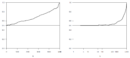
In Figure 2 we present a sample path of the estimator η^nsubscript^𝜂𝑛\widehat{\eta}_{n} in (2.4) as a function of k1,𝑘1k\geq 1, for a sample of size n=5000𝑛5000n=5000 in a linear scale and in a logarithmic scale.
Refer to caption
Figure 2: Sample path of the upcrossings index estimator as a function of k𝑘k for a sample of size n=5000𝑛5000n=5000 from the stationary ARMAX process in (6.1), in a linear scale (left) and in a logarithmic scale (right).

As we can see from Figure 2 the logarithmic scale enhances the performance of η^nsubscript^𝜂𝑛\widehat{\eta}_{n} for small values of k,𝑘k, giving better insight of its stability region around η=0.5𝜂0.5\eta=0.5.

For samples of size n=100,200,500,1000,2000,5000𝑛100200500100020005000n=100,200,500,1000,2000,5000 and 10000, from the ARMAX process in (6.1), we have performed a multi-sample Monte Carlo simulation with 5000 runs and 10 replicates. For details on multi-sample simulation see, for instance, Gomes and Oliveira [8]. We have simulated for the estimator η^n(k)subscript^𝜂𝑛𝑘\widehat{\eta}_{n}(k) in (2.4), the mean value (E𝐸E), the mean squared error (MSE𝑀𝑆𝐸MSE) and the optimal sample fraction k0subscript𝑘0k_{0} with k0:=argminkMSE[η^n(k)].assignsubscript𝑘0subscript𝑘𝑀𝑆𝐸delimited-[]subscript^𝜂𝑛𝑘k_{0}:=\arg\min_{k}MSE[\widehat{\eta}_{n}(k)].

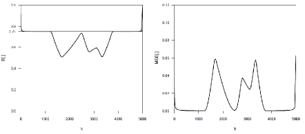
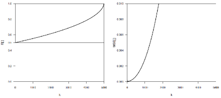
In Figure 3, we illustrate the values of the estimated mean values and MSE’s of η^n(k)subscript^𝜂𝑛𝑘\widehat{\eta}_{n}(k) in (2.4), for a sample of size n=5000𝑛5000n=5000 from the ARMAX process in (6.1), with upcrossings index η=0.5.𝜂0.5\eta=0.5. In Table 1 we present the main distributional properties of the estimator under study with the associated 95% confidence intervals (see Gomes and Oliveira [8] ).
Refer to caption
Figure 3: Estimated mean values (left) and mean squared errors (right), for samples of size n=5000𝑛5000n=5000 from the ARMAX process in (6.1) (η=0.5𝜂0.5\eta=0.5)
n𝑛n k0subscript𝑘0k_{0} k0/nsubscript𝑘0𝑛k_{0}/n E[]𝐸delimited-[]E[\bullet] MSE[]𝑀𝑆𝐸delimited-[]MSE[\bullet] SD[]𝑆𝐷delimited-[]SD[\bullet]
100100100 161616 0.1600.1600.160 0.52735±0.00042plus-or-minus0.527350.000420.52735\pm 0.00042 0.00497±0.000087plus-or-minus0.004970.0000870.00497\pm 0.000087 0.06495±0.00064plus-or-minus0.064950.000640.06495\pm 0.00064
200200200 191919 0.0950.0950.095 0.51754±0.00029plus-or-minus0.517540.000290.51754\pm 0.00029 0.00214±0.000029plus-or-minus0.002140.0000290.00214\pm 0.000029 0.04282±0.00037plus-or-minus0.042820.000370.04282\pm 0.00037
500500500 252525 0.0500.0500.050 0.50977±0.00021plus-or-minus0.509770.000210.50977\pm 0.00021 0.00072±0.000018plus-or-minus0.000720.0000180.00072\pm 0.000018 0.02493±0.00030plus-or-minus0.024930.000300.02493\pm 0.00030
100010001000 303030 0.0300.0300.030 0.50622±0.00014plus-or-minus0.506220.000140.50622\pm 0.00014 0.00033±0.000008plus-or-minus0.000330.0000080.00033\pm 0.000008 0.01699±0.00022plus-or-minus0.016990.000220.01699\pm 0.00022
200020002000 363636 0.0180.0180.018 0.50389±0.00007plus-or-minus0.503890.000070.50389\pm 0.00007 0.00015±0.000003plus-or-minus0.000150.0000030.00015\pm 0.000003 0.01162±0.00013plus-or-minus0.011620.000130.01162\pm 0.00013
500050005000 545454 0.0110.0110.011 0.50241±0.00006plus-or-minus0.502410.000060.50241\pm 0.00006 0.00005±0.000001plus-or-minus0.000050.0000010.00005\pm 0.000001 0.00694±0.00010plus-or-minus0.006940.000100.00694\pm 0.00010
100001000010000 676767 0.0070.0070.007 0.50152±0.00003plus-or-minus0.501520.000030.50152\pm 0.00003 0.00003±0.000001plus-or-minus0.000030.0000010.00003\pm 0.000001 0.00477±0.00006plus-or-minus0.004770.000060.00477\pm 0.00006
Table 1: Optimal sample fractions, mean values and mean squared errors of the estimator at its optimal levels, for the ARMAX process, with η=0.5.𝜂0.5\eta=0.5.

6.2 AR(1) process

Lets consider the negatively correlated uniform AR(1) process of Chernick et al. [2],

Xn=1rXn1+ϵn,n1,formulae-sequencesubscript𝑋𝑛1𝑟subscript𝑋𝑛1subscriptitalic-ϵ𝑛𝑛1X_{n}=-\frac{1}{r}X_{n-1}+\epsilon_{n},\quad n\geq 1, (6.2)

where {ϵn}n1subscriptsubscriptitalic-ϵ𝑛𝑛1\{\epsilon_{n}\}_{n\geq 1} is a sequence of independent and identically distributed random variables, such that, for a fixed integer r2,𝑟2r\geq 2, ϵnU{1r,,r1r,1}similar-tosubscriptitalic-ϵ𝑛𝑈1𝑟𝑟1𝑟1\epsilon_{n}\sim U\{\frac{1}{r},\ldots,\frac{r-1}{r},1\} and X0U(0,1)similar-tosubscript𝑋0𝑈01X_{0}\sim U(0,1) independent of ϵn.subscriptitalic-ϵ𝑛\epsilon_{n}.

Condition D~(3)(𝐮)superscript~𝐷3𝐮\widetilde{D}^{(3)}({\bf{u}}) also holds for this stationary sequence, with 𝐮=𝐮(ν)={un=1τ/n}n1,𝐮superscript𝐮𝜈subscriptsubscript𝑢𝑛1𝜏𝑛𝑛1{\bf{u}}={\bf{u}}^{(\nu)}=\{u_{n}=1-\tau/n\}_{n\geq 1}, τ>0,𝜏0\tau>0, moreover limn+nP(X1>un)=τsubscript𝑛𝑛𝑃subscript𝑋1subscript𝑢𝑛𝜏\lim_{n\to+\infty}nP(X_{1}>u_{n})=\tau and η=θ=11/r2𝜂𝜃11superscript𝑟2\eta=\theta=1-1/r^{2} (see Sebastião et al. [18]). Condition D′′(𝐮)superscript𝐷′′𝐮D^{\prime\prime}({\bf{u}}) typically doesn’t hold for these sequences since they tend to oscillate rapidly near extremes. To illustrate this characteristic we present in Figure 4 sample paths of the negatively correlated uniform AR(1) processes for r=2,𝑟2r=2, r=3𝑟3r=3 and r=5𝑟5r=5 (η=θ=0.75,𝜂𝜃0.75\eta=\theta=0.75, η=θ=0.89𝜂𝜃0.89\eta=\theta=0.89 and η=θ=0.96,𝜂𝜃0.96\eta=\theta=0.96, respectively).

Refer to caption
Figure 4: Sample paths of the stationary AR(1) process in (6.2), with r=2𝑟2r=2 (left), r=3𝑟3r=3 (center) and r=5𝑟5r=5 (right)

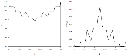
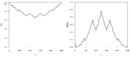
We present, in Figures 5-7, the estimated mean values and MSE’s of η^n(k)subscript^𝜂𝑛𝑘\widehat{\eta}_{n}(k) in (2.4), for a sample of size n=5000𝑛5000n=5000 from the AR(1) process in (6.2), with upcrossings index η=0.75, 0.89𝜂0.750.89\eta=0.75,\ 0.89 and 0.96, respectively.

r=2𝑟2r=2
Refer to caption
r=3𝑟3r=3
Refer to caption
r=5𝑟5r=5
Refer to caption
Figure 5: Estimated mean values (left) and mean squared errors (right), for samples of size n=5000𝑛5000n=5000 from the AR(1) process in (6.2) with, respectively, r=2𝑟2r=2 (η=0.75𝜂0.75\eta=0.75), r=3𝑟3r=3 (η=0.89𝜂0.89\eta=0.89) and r=5𝑟5r=5 (η=0.96𝜂0.96\eta=0.96)

In Table 2 we present the main distributional properties of the estimator under study with the associated 95% confidence intervals.

n𝑛n k0subscript𝑘0k_{0} k0/nsubscript𝑘0𝑛k_{0}/n E[]𝐸delimited-[]E[\bullet] MSE[]𝑀𝑆𝐸delimited-[]MSE[\bullet]
𝜼=0.75𝜼0.75{\boldsymbol{\eta}}{\bf{=0.75}}
100100100 242424 0.2400.2400.240 0.72839±0.00081plus-or-minus0.728390.000810.72839\pm 0.00081 0.00769±0.000075plus-or-minus0.007690.0000750.00769\pm 0.000075
200200200 494949 0.2450.2450.245 0.73228±0.00043plus-or-minus0.732280.000430.73228\pm 0.00043 0.00364±0.000055plus-or-minus0.003640.0000550.00364\pm 0.000055
500500500 123123123 0.2460.2460.246 0.73942±0.00026plus-or-minus0.739420.000260.73942\pm 0.00026 0.00140±0.000016plus-or-minus0.001400.0000160.00140\pm 0.000016
100010001000 246246246 0.2460.2460.246 0.74375±0.00009plus-or-minus0.743750.000090.74375\pm 0.00009 0.00068±0.000009plus-or-minus0.000680.0000090.00068\pm 0.000009
200020002000 494494494 0.2470.2470.247 0.74576±0.00017plus-or-minus0.745760.000170.74576\pm 0.00017 0.00034±0.000005plus-or-minus0.000340.0000050.00034\pm 0.000005
500050005000 124012401240 0.2480.2480.248 0.74745±0.00010plus-or-minus0.747450.000100.74745\pm 0.00010 0.00013±0.000002plus-or-minus0.000130.0000020.00013\pm 0.000002
𝜼=0.89𝜼0.89{\boldsymbol{\eta}}{\bf{=0.89}}
100100100 101010 0.1000.1000.100 0.86547±0.00112plus-or-minus0.865470.001120.86547\pm 0.00112 0.01254±0.000240plus-or-minus0.012540.0002400.01254\pm 0.000240
200200200 191919 0.0950.0950.095 0.87623±0.00077plus-or-minus0.876230.000770.87623\pm 0.00077 0.00598±0.000096plus-or-minus0.005980.0000960.00598\pm 0.000096
500500500 484848 0.0960.0960.096 0.88347±0.00029plus-or-minus0.883470.000290.88347\pm 0.00029 0.00221±0.000025plus-or-minus0.002210.0000250.00221\pm 0.000025
100010001000 989898 0.0980.0980.098 0.88642±0.00017plus-or-minus0.886420.000170.88642\pm 0.00017 0.00105±0.000009plus-or-minus0.001050.0000090.00105\pm 0.000009
200020002000 201201201 0.1010.1010.101 0.88768±0.00020plus-or-minus0.887680.000200.88768\pm 0.00020 0.00050±0.000007plus-or-minus0.000500.0000070.00050\pm 0.000007
500050005000 519519519 0.1040.1040.104 0.88842±0.00007plus-or-minus0.888420.000070.88842\pm 0.00007 0.00019±0.000003plus-or-minus0.000190.0000030.00019\pm 0.000003
𝜼=0.96𝜼0.96{\boldsymbol{\eta}}{\bf{=0.96}}
100 7 0.070 0.91442±0.00123plus-or-minus0.914420.001230.91442\pm 0.00123 0.01431±0.000366plus-or-minus0.014310.0003660.01431\pm 0.000366
200 9 0.045 0.93962±0.00081plus-or-minus0.939620.000810.93962\pm 0.00081 0.00728±0.000126plus-or-minus0.007280.0001260.00728\pm 0.000126
500 17 0.034 0.95373±0.00072plus-or-minus0.953730.000720.95373\pm 0.00072 0.00274±0.000077plus-or-minus0.002740.0000770.00274\pm 0.000077
1000 33 0.033 0.95687±0.00054plus-or-minus0.956870.000540.95687\pm 0.00054 0.00130±0.000038plus-or-minus0.001300.0000380.00130\pm 0.000038
2000 67 0.034 0.95842±0.00026plus-or-minus0.958420.000260.95842\pm 0.00026 0.00061±0.000011plus-or-minus0.000610.0000110.00061\pm 0.000011
5000 173 0.035 0.95949±0.00017plus-or-minus0.959490.000170.95949\pm 0.00017 0.00023±0.000004plus-or-minus0.000230.0000040.00023\pm 0.000004
Table 2: Optimal sample fractions, mean values and mean squared errors of the estimator at its optimal levels, for the AR(1) process, with η=0.75,𝜂0.75\eta=0.75, η=0.89𝜂0.89\eta=0.89 and η=0.96𝜂0.96\eta=0.96.

6.3 Some overall conclusions

  • The sample paths of the runs estimator of the upcrossings index have very different patterns for the ARMAX and the AR(1) process. Whilst for the ARMAX process the estimates increase with the value of k,𝑘k, for the AR(1) process the estimates, as function of k,𝑘k, have almost a symmetric distribution, decreasing with smaller values of k.𝑘k.

  • For the ARMAX process, smaller values of η𝜂\eta tend to be associated with a wider “bathtub” pattern of the mean squared error as a function of k.𝑘k.

  • The runs estimator of the upcrossings index has some mean value stability around the target η𝜂\eta for small values of k,𝑘k, exhibiting, for such values, the mean squared error a “bathtub” pattern, although not very wide.

  • For small values of k,𝑘k, or equivalently high levels, we obtain good estimates for η.𝜂\eta. We remark that the choice of the number of top order statistics is a complex problem in extreme value applications.

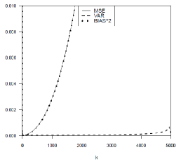
  • The sensitivity of the mean value to the changes in k𝑘k seem to clarify the need of studying the bias properties of this estimator. This is clear form Figure 6 where we can see that for the ARMAX process the behaviour of the mean squared error is almost determined by the bias (overlap of both curves), since the variance is always very small. The same behaviour holds for the AR(1) process.
    Refer to caption
    Figure 6: Estimated mean squared error (solid line), estimated variance (dashed line) and estimated bias (dotted line), for samples of size n=5000𝑛5000n=5000 from the ARMAX process in (6.1).

7 Case-studies

7.1 Ozone pollution

We now consider the performance of the above mentioned estimator in the analysis of n=120𝑛120n=120 weekly maxima of hourly averages of ozone concentrations measured in parts per million, in the San Francisco bay area, San José. These data are available in the package Xtremes (Reiss and Thomas [16]) and have already been studied, for instance, in Gomes et al. [7] when estimating the extremal index. In Figure 7 we picture the data over the above mentioned period.

Refer to caption
Figure 7: Weekly maxima of hourly averages of ozone concentrations measured in parts per million, in the San Francisco bay area, San José

Since in practice condition D~(3)superscript~𝐷3\widetilde{D}^{(3)} is not yet possible to verify we assumed that it holds since as stated Gomes et al. [7], most of the parametric models that adequately fit this type of meteorological data satisfy condition D′′superscript𝐷′′D^{\prime\prime} and therefore also satisfy condition D~(3).superscript~𝐷3\widetilde{D}^{(3)}.

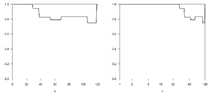
In Figure 8 we picture the sample paths of η^n(k)subscript^𝜂𝑛𝑘\widehat{\eta}_{n}(k) as functions of k𝑘k in a linear scale (left) and logarithmic (right) scale.
Refer to caption
Figure 8: Estimates of the upcrossings index as a function of k𝑘k for the weekly maxima of hourly averages of ozone concentrations measured in parts per million, in the San Francisco bay area, San José, in a linear scale (left) and in a logarithmic scale (right).

The stability around one for small values of k𝑘k agrees with the fact that η=1𝜂1\eta=1 since from [7] condition D′′superscript𝐷′′D^{\prime\prime} holds. Nevertheless, the small number of observations makes it difficult to rely on such a point estimate since the number of upcrossings and consequently the number of non-upcrossings followed by an upcrossing, of a hight level, will always be very small.

7.2 Financial log-returns

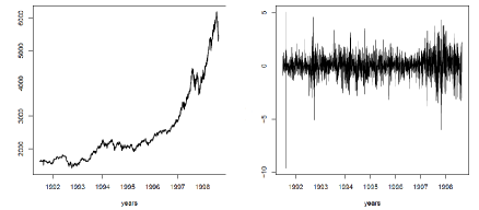
Financial time series are very unlikely to satisfy condition D′′superscript𝐷′′D^{\prime\prime} because of their varying volatility. Therefore, we shall consider now the time series of log returns of the German stock market index DAX, consisting of the 30 major German companies trading on the Frankfurt Stock Exchange. The daily closing prices of the DAX index for the period from 1991 to 1998 that we work with is available as dataset EuStockMarkets in the statistics software R, which we also used for all computations. This data set of 1786 observations has been considered in Klar at al. [10] where we can find a full statistical description. In Figure 9 we picture DAX daily closing prices over the mentioned period, xt,subscript𝑥𝑡x_{t}, and the log-returns, 100×(lnxtlnxt1),100subscript𝑥𝑡subscript𝑥𝑡1100\times(\ln x_{t}-\ln x_{t-1}), the data to be analyzed.

Refer to caption
Figure 9: DAX daily closing prices (left) and daily log-returns (right)

This time series of log returns is well modeled by a GARCH(1,1), covariance stationary, process ([10]). Using a goodness-of-fit test Klar at al. [10], at a 5% level, do not reject the hypothesis that the innovations of the process follow a t-distribution with seven degrees of freedom.
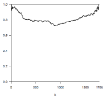
Refer to caption
Figure 10: Estimates of the upcrossings index as a function of k𝑘k for the DAX log-returns

The graph in Figure 10 allows us to conclude that η𝜂\eta is not equal to one, which agrees with the fact that these processes are very unlikely to verify condition D′′.superscript𝐷′′D^{\prime\prime}. The sample path exhibits a stability region around a value close to η=0.8.𝜂0.8\eta=0.8.

Mikosch and Stărică [14] derive the extremal index for the squared GARCH(1,1) processes, whereas Laurini and Tawn [11] propose an algorithm for the evaluation of the extremal index of GARCH(1,1) processes with tlimit-from𝑡t-distributed innovations. It would be interesting, in future work, to obtain similar results for the upcrossings index of a GARCH(1,1) process.

8 Conclusions

The upcrossings index, as a measure of the clustering of upcrossings of high levels, is an important parameter when studying extreme events. For sequences satisfying condition D~(3),superscript~𝐷3\widetilde{D}^{(3)}, that locally restricts the dependence of the sequence but still allows clustering of upcrossings, we have proposed a simple estimator for this parameter. The study of the properties of the proposed estimator, namely its consistency and asymptotic normality, has been carried out in Sections 3 and 4. With simulations of well known autoregressive processes that verify condition D~(3)superscript~𝐷3\widetilde{D}^{(3)} we were able to illustrate the performance of the estimator. Case studies in the fields of environment and finance were also exploited.

Relation (1.5) allows one also to estimate η𝜂\eta through the extremal index θ𝜃\theta modified by consistent estimators of exceedances, τ𝜏\tau, and the mean number of upcrossings, ν,𝜈\nu, of high levels. Several estimators for the extremal index can be found in the literature (see Ancona-Navarrete and Tawn [1] for a survey). Other estimators arise from Proposition 1.1 and from the relation with μ1,subscript𝜇1\mu_{1}, the upcrossings-tail dependence coefficient. In future work we intend to propose new estimators for the upcrossings index and compare the several estimating methods.

References

  • [1] Ancona-Navarrete, M. A. and Tawn, J. A. (2000). A comparison of methods for estimating the extremal index. Extremes, 3(1), 5-38.
  • [2] Chernick, M., Hsing, T. and McCormick, W. (1991). Calculating the extremal index for a class of stationary sequences. Adv. Appl. Prob., 23, 835-850.
  • [3] Feller, W. (1971). An Introduction to Probability Theory and Its Applications. New York: Wiley.
  • [4] Ferreira. H. (2006). The upcrossing index and the extremal index. J. Appl. Prob., 43, 927-937.
  • [5] Ferreira, H. (2007). Runs of high values and the upcrossings index for a stationary sequence. Em Proceedings of the 56th Session of the ISI.
  • [6] Ferreira, M. and Ferreira, H. (2011). On extremal dependece: some contributions. Test. DOI: 10.1007/s11749-011-0261-3.
  • [7] Gomes, M.I., Hall, A. and Miranda, C. (2008). Subsampling techniques and the Jacknife methodology in the estimation of the extremal index. J. Statist. Comput. Simulation, 52, 2022-2041.
  • [8] Gomes, M.I. and Oliveira, O. (2001). The boostrap methodology in Statistics of extremes - choice of the optimal sample fraction. Extremes, 4(4), 331-358.
  • [9] Hsing, T., Hüsler, J. and Leadbetter, M.R. (1988). On the exceedance point process for a stationary sequence. Prob. Th. Rel. Fields, 78, 97-112.
  • [10] Klar, B., Lindner, F. and Meintanis, S.G. (2011). Specification tests for the error distribution in Garch models. Computational Statistics and Data Analysis. DOI:10.1016/j.csda.2010.05.029
  • [11] Laurini, F. and Tawn, J. (2006). The extremal index for GARCH(1,1) processes with t-distributed innovationas. http://www.scientificcommons.org/17368349
  • [12] Leadbetter, M.R. (1974). On extreme values in stationary sequences. Z. Wahrsch. Verw. Gebiete, 28, 289-303.
  • [13] Leadbetter, M. R. and Nandagopalan, S. (1988). On exceedance point process for stationary sequences under mild oscillation restrictions. In J. Hüsler and D. Reiss (eds.). Extreme Value Theory: Proceedings, Oberwolfach 198719871987, Springer, New York, 69-80.
  • [14] Mikosch, T. and Stărică, C. (2000). Limit theory for the sample autocorrelations and extremes of a GARCH(1,1) process. Ann. Statist., 28, 1427-1451.
  • [15] Nandagopalan, S. (1990). Multivariate Extremes and Estimation of the Extremal Index. Ph.D. Thesis, University of North Carolina. Chapel Hill.
  • [16] Reiss, R.-D. and Thomas, M. (2007). Statistical Analysis of Extreme Values with Apllications to Insurance, Finance, Hydology and Other Fields. Birkhäuser Verlag, Basel, Switzerland.
  • [17] Ross, S. (1983). Stochactic Processes. New York: Wiley.
  • [18] Sebastião, J., Martins, A.P., Pereira, L. and Ferreira. H., (2010). Clustering of upcrossings of high values. J. Statist. Plann. Inf., 140, 1003–1012