Agglomerative Percolation on Bipartite Networks: A Novel Type of Spontaneous Symmetry Breaking

Abstract

Ordinary bond percolation (OP) can be viewed as a process where clusters grow by joining them pairwise, by adding links chosen randomly one by one from a set of predefined ‘virtual’ links. In contrast, in agglomerative percolation (AP) clusters grow by choosing randomly a ‘target cluster’ and joining it with all its neighbors, as defined by the same set of virtual links. Previous studies showed that AP is in different universality classes from OP for several types of (virtual) networks (linear chains, trees, Erdös-Rényi networks), but most surprising were the results for 2-d lattices: While AP on the triangular lattice was found to be in the OP universality class, it behaved completely differently on the square lattice. In the present paper we explain this striking violation of universality by invoking bipartivity. While the square lattice is a bipartite graph, the triangular lattice is not. In conformity with this we show that AP on the honeycomb and simple cubic (3-d) lattices – both of which are bipartite – are also not in the OP universality classes. More precisely, we claim that this violation of universality is basically due to a $Z_{2}$ symmetry that is spontaneously broken at the percolation threshold. We also discuss AP on bipartite random networks and suitable generalizations of AP on $k-$partite graphs.

I Introduction

Percolation was until recently considered a mature subject that held few surprises, but this has changed dramatically during the last few years. Recent discoveries that widened enormously the scope of different behaviors at the percolation threshold include infinite order transitions in growing networks callaway , supposedly first order transitions in Achlioptas processes Achli-2009 (that are actually continuous Costa-2010 ; Riordan but show very unusual finite size behavior Grassberger ), and real first order transitions in interdependent networks Buldy-2010 ; Parshani-2010 ; Son-2011 ; Son-PRL-2011 . Another class of “non-classical” percolation models, inspired by attempts to formulate a renormalization group for networks Song-2005 ; Radic-2009 , was introduced in Bizh-2010 ; Christen-2010 ; Son-2010 ; Son-EPL-2011 ; Bizhani-PRE-2011 and is called ‘agglomerative percolation’ (AP).

The prototype model in the ordinary percolation (OP) universality class is bond percolation Stau-1994 . There one starts with a set of $N$ nodes and a set of ‘virtual’ links between them, i.e. links that can be placed but that are not yet put down. One then performs a process where one repeatedly picks at random one of the virtual bonds and realizes it, i.e. actually links the two nodes. A giant cluster appears with probability one in the limit $N\to\infty$, when the density $p=M/N$ of links ($M$ is here the number of realized links) exceeds a threshold $p_{c}$ whose value depends on the topology of the network. The behavior at $p\approx p_{c}$ is governed by ‘universal’ scaling laws, i.e. by scaling laws with exponents that depend only on few gross properties of the network. A typical example is that the universality class of OP on regular $d-$dimensional lattices depends on $d$ but not on the lattice type. For example, OP on triangular and square lattices (both have $d=2$) are in the same universality class.

AP differs from OP in that clusters do not grow by establishing links one by one. Rather, one picks a ‘target’ cluster at random (irrespective of its mass; we are dealing here with model (a) in the classification of Christen-2010 ) and joins it with all its neighbors, where neighborhoods are defined by the virtual links. The new combined cluster is then linked to all neighbors of its constituents. AP can be solved rigorously on 1-d linear chains Son-2010 ; Son-EPL-2011 , where it is found to be in a different universality class from OP. Although a similarly complete mathematical analysis is not possible on random graphs, both numerics and non-rigorous analytical arguments show that the same is true for ‘critical’ trees Bizh-2010 and Erdös-Rényi graphs Bizhani-PRE-2011 .

In contrast to these cases that establish AP as a novel phenomenon but do not present big surprises, the behavior on 2-d regular lattices Christen-2010 is extremely surprising: While AP on the triangular lattice is clearly in the OP universality class (with only some minor caveats), it behaves completely different on the square lattice. There the average cluster size at criticality diverges as the system size $L$ increases (it stays finite for all realizations of OP on any regular lattice), the fractal dimension of the incipient giant cluster is $D_{f}=2$ ($D_{f}=91/48\approx 1.90$ for OP), and the cluster mass distribution obeys a power law with power $\tau=2$ ($\tau=187/91\approx 2.055$ for OP). This blatant violation of universality – one of the most cherished results of renormalization group theory – is, as far as we know, unprecedented.

As we said above, gross topological features of the network (such as dimensionality in case of regular lattices, the correlations between links induced by growing networks callaway , and finite ramification in hierarchical graphs Boettcher-2011 ) are one set of properties that determine universality classes. The other features that determine universality classes in general are symmetries of the order parameter: The Ising and Heisenberg models are in different universality classes, e.g., because the order parameter is a scalar in the first and a 3-d vector in the second. Could it be that the non-universality of AP results from a similar symmetry? At first sight this seems unlikely, because the order parameter (the density of the giant cluster) is a scalar in any percolation model. Moreover, in order for a symmetry to affect the universality class it has to be broken spontaneously at the phase transition.

In the following we show that it is indeed the latter scenario that leads to the non-universality of AP on square and triangular lattices, and the symmetry that is spontaneously broken at the AP threshold on the square lattice is a $Z_{2}$ symmetry resulting from bipartivity. A graph is bipartite, if the set ${\cal N}$ of nodes can be split into two disjoint subsets, ${\cal N}={\cal N}_{1}\sqcup{\cal N}_{2}$, such that all links are connecting a node in ${\cal N}_{1}$ with a node in ${\cal N}_{2}$, and there are no links within ${\cal N}_{1}$ or within ${\cal N}_{2}$. A square lattice is bipartite (as illustrated by the black/white colors of a checkerboard), but a triangular lattice is not. Following this example, we will in the following speak of the different colors of the sets ${\cal N}_{1}$ and ${\cal N}_{2}$. The initial state of the AP process on a square lattice (where each site is a cluster) is color symmetric. If the AP cluster joining process is such that we can attribute a definite color to any cluster (even when it is not a single site), then the state remains color symmetric until we reach a state with a giant cluster. In this state the color symmetry is obviously broken.

In Sec. 2 we shortly review the evidence for non-universality given in Christen-2010 , In Sec. 3 we present new results which show that AP on square lattices behaves even more strange than found before. There we also present numerical results for the honeycomb and simple cubic lattices, both of which are bipartite and show similar anomalies as the square lattice. The detailed explanation why bipartivity leads to these results is given in Sec. 4. Random bipartite networks are shortly treated in Sec. 5. Possible generalizations to $k$-partite graphs with $k>2$ are discussed in Sec. 6, while we finish with our conclusions in Sec. 7.

II Agglomerative Percolation: Definition, implementation, and review of previous results

We start with a graph with $N$ nodes and $M$ links. Clusters are defined trivially in this initial state, i.e. each node is its own cluster. AP is then defined by repeating the following step until one single cluster is left:

1) Pick randomly one of the clusters with uniform probability;
2) Join this ‘target cluster’ with all its neighboring clusters, where two clusters $C_{1}$ and $C_{2}$ are ‘neighbors’, if there exist a pair of nodes $i\in C_{1}$ and $j\in C_{2}$ that are joined by a link;

As described in Christen-2010 , this is implemented most efficiently with the Newman-Ziff algorithm Newman-2001 that uses pointers to point to the “roots” of clusters, augmented by a breadth-first search to find all neighbors of the target.

In ordinary bond percolation one usually takes as control parameter $p$ the number of established (i.e. non-virtual) links, divided by the number of all possible links (including virtual ones). This is not practical for AP. Rather, we use as in Ziff-2009 ; Christen-2010 the number $n$ of clusters per node. It was checked carefully in these papers that using $n$ instead of $p$ as a control parameter in ordinary bond percolation is perfectly legitimate, since one is a smooth monotonic (decreasing) function of the other.

In Christen-2010 , AP was studied on two different 2-d lattices. Helical boundary conditions were used for both, i.e. sites are labeled by a single index $i$ with $i\equiv(i\;\;{\rm mod}\;\;L^{2}$, where $L$ is the lattice size). For the square lattice the four neighbors of site $i$ are $i\pm 1$ and $i\pm L$, while there are two additional neighbors $i\pm(L+1)$ for the triangular lattice. This seemingly minor difference has dramatic consequences. While AP on the triangular lattice is (within statistical errors, and with one minor caveat that was easily understood) in the universality class of OP, this is obviously not the case for the square lattice. Among other results, the following results were found:

Figure 1: (Color online) Effective critical cluster densities for AP on finite 2-d lattices versus $L^{-3/4}$, where $L$ is the lattice size. For ordinary percolation, where $n_{c}(L)-n_{c}\sim L^{-1/\nu}$ with $\nu=4/3$, this should give straight lines. For each lattice type (triangular: upper pair of curves; square: lower pair of curves) we show results obtained with two different operational definitions for the critical point: (i) Maximal range of the power law $P_{n}(m)\sim m^{-\tau}$, and (ii) the probability to have a cluster that wraps around a lattice with helical boundary conditions is equal to 1/2. The corresponding values of $n_{c}(L)$ are called $n_{c,\tau}(L)$ and $n_{c,{\rm wrap}}(L)$ (from Ref. Christen-2010 ).

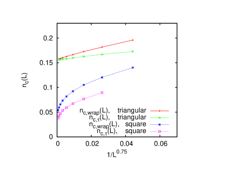
• The effective percolation threshold – measured either by the probability that a cluster wraps around the lattice, or via the best scaling law

  $$P(m)\sim m^{-\tau}$$ (1)

  for the probability distribution of cluster masses $m$ – depends strongly on $L$. For OP this dependence is governed by the correlation length exponent $\nu$ via

  $$p_{c}-p_{c}(L)\propto n_{c}(L)-n_{c}\propto L^{-1/\nu}$$ (2)

  with $\nu=4/3$ and $n_{c}>0$. The latter means, in particular, that the average cluster size is finite at criticality. For AP on the square lattice a parameterization like this would give $\nu=0$. More precisely, $n_{c}(L)$ seems to decrease logarithmically to a value $n_{c}=0$, i.e. the average cluster at criticality (and in the limit $L\to\infty$) is zero. This is summarized in Fig. 1.

• The exponent $\tau$ in Eq. (1), which is $187/91=2.0549\ldots$ for OP, seems to be $<2$ at first sight. But it slowly increases with $L$, and it was argued that the exact value is $\tau=2$.

• Similarly, the fractal dimension of the largest cluster was measured as $\approx 1.95$, while it is $D_{f}=91/48=1.9858\ldots$ for OP. It also increases slowly with $L$, and it was conjectured that also $D_{f}=2$.

• Let $p_{\rm wrap}(n,L)$ be the probability that there exists a cluster that wraps along the vertical direction on a lattice of size $L$, when there are $nL^{2}$ clusters. The distribution $dp_{\rm wrap}(n)/dn$ is universal for OP. For AP on triangular lattices it develops a weak tail for small $n$ (this is the easily explained caveat mentioned above), but for AP on the square lattice it has a very fat tail for small $n$. Thus there is a high probability that even at very late stages in the agglomeration process, when only few clusters remain, none of them has yet wrapped.

III Additional numerical results

III.1 Square lattice

III.1.1 Periodic boundary conditions

Helical b.c. were used in Christen-2010 simply for convenience (they are more easy to code than periodic ones), and it was assumed that the small difference with strictly periodic b.c. should be without any consequences. This is not true. Not only is there a large difference between helical and strictly periodic b.c.’s (even for the largest values of $L$ that we could check), but for the latter there is an even stronger difference between even and odd $L$.

Figure 2: (Color online) Wrapping probability density $dp_{\mathrm{wrap}}/dn$ for 2D square lattices with different boundary condition, and with sizes differing by just one unit, compared to similar results for triangular lattices. All curves for square lattices have peaks at smaller values than for triangular lattices and have more heavy left hand tails, but this is most pronounced for strictly periodic b.c. with even $L$.

Figure 3: (Color online) Black triangles: Cluster densities $n$ at which $p_{\rm wrap}(n)=1/2$, plotted against $L$, for square lattices with periodic b.c. The upper curve is for odd sizes, and the lower curve is for even sizes. Red dots: Analogous results for a slightly modified model, where each neighboring cluster agglomerates with the target cluster only with probability $q<1$. In the present case $q=0.999$.

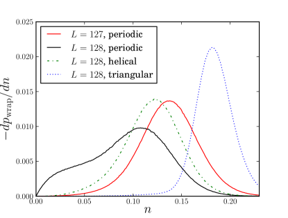
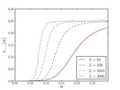
In Fig. 2 we show $dp_{\rm wrap}(n)/dn$ for four different cases:
(i) Triangular lattices. The shape of this curve is practically indistinguishable from ordinary percolation, and serves as a reference for the latter.
(ii) Square lattices of size $128\times 128$ with helical b.c. Compared to the triangular lattice, there is a much fatter left hand tail of the distribution, i.e. there are many more realizations where no cluster has yet wrapped, although the number of clusters is very small.
(iii) Square lattices of the same size, but with periodic b.c. Now the left hand tail is even more fat. Indeed, for this lattice size one finds realizations with $\leq 10$ clusters, none of which has yet wrapped.
(iv) Square lattices of sizes $127\times 127$ with periodic b.c. We see a huge difference, in spite of the small change in $L$, making the results similar to those for helical b.c. Obviously, this indicates a distinction between even and odd $L$.

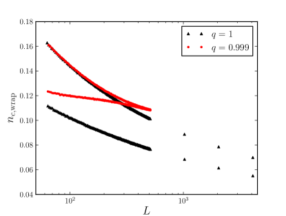
The last conclusion is confirmed by Fig. 3. There we show the values of $n$ where half of the configurations have wrapping clusters, $p_{\rm wrap}(n)=1/2$ (black triangles; the red dots will be discussed in subsection III.1.2). These data confirm that the difference between even and odd $L$ persists even to our largest systems, where the difference in $L$ between the two is less than 0.025 per cent.

III.1.2 Finite agglomeration probability

In AP, all neighbors of a chosen target are included in each agglomeration step. In contrast, bond percolation can be viewed as the limit $q\to 0$ of a model where each neighbor is included with probability $q$. One might then wonder where the cross-over from OP to AP happens. Is it for $q\to 0$ (meaning that the model is in the AP universality class for any $q>0$), for $q\to 1$ (in which case we have OP for any $q<1$), or for some $0<q<1$?

The numerical answer is clear and surprising in its radicalness: For any $q<1$ we find OP, if we go to large enough $L$, even if $q=0.999$ (see Fig. 3). More precisely, we see that the difference between even and odd $L$ disappears rapidly when $L$ increases, and both curves seem to converge to a finite $n_{c,\rm wrap}$ for $L\to\infty$. It seems that even the slightest mistake in the agglomeration process completely destroys the phenomenon and places the model in the OP universality class.

This is confirmed by looking at the order parameter

$$S=\langle m_{\rm max}\rangle/N$$ (3)

where $m_{\rm max}$ is the size of the largest cluster. For infinite systems, $S=0$ for $n>n_{c}$ and $S>0$ for $n<n_{c}$. For OP, one has $S\sim(n_{c}-n)^{\beta}$ for $n$ slightly below $n_{c}$, and the usual finite size scaling (FSS) behavior

$$S\sim L^{\beta/\nu}f[(n_{c}-n)L^{1/\nu}]$$ (4)

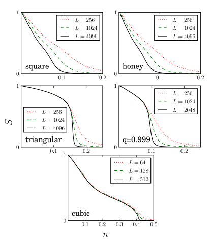
for finite systems. In Fig. 4 we show $s$ versus $n$ for various cases, all with periodic b.c. In addition to two panels for other lattices discussed in later subsections (“honey”, “cubic”) we show results for the triangular lattice and for square lattices with $q=1$ (“square”) and with $q=0.999$. We see that the results for $q<1$ are very similar to those for the triangular lattice, while they are completely different from those for $q=1$. A data collapse for verifying the FSS ansatz would of course not be perfect, but it seems that the model with $q<1$ is in the OP universality class, for any $q<1$.

Figure 4: (Color online) The five panels of this figure correspond to (i) square lattices with $q=1$, (ii) honeycomb lattices, (iii) triangular lattices, (iv) square lattices with $q=0.999$, and (v) cubic lattices. In all cases, periodic b.c. were used. In all cases except case (iv), $q=1$.

III.2 Other regular lattices

In addition to the square and triangular lattices we now study also the honeycomb lattice as a third lattice with $d=2$, and the simple cubic lattice as an example of a 3-d lattice.

III.2.1 Honeycomb lattice

Although we measured also other observables (such as the wrapping probabilities), we show here only the behavior of the order parameter $S$. As seen in Fig. 4, the behavior here is very similar to that for the square lattice. In particular, we see no indication for the FSS ansatz with finite (non-zero) $n$.

III.2.2 3-d simple cubic lattice

The behavior on the simple cubic lattice is more subtle. On the one hand, we clearly see in Fig. 4 an indication for a non-zero value of $n_{c}$, with $n_{c}\approx 0.41$. On the other hand, as for the square and honeycomb lattices we see that the slope $dS/dn$ is not monotonic. In all three cases the growth of the largest cluster slows down when $S\approx 1/4$, and accelerates again when $S>1/2$. Alternatively, it seems as if two behaviors are superimposed: For large $n$ and $S<1/3$ it seems as if the curves would extrapolate to $S=1/2$ for $n\to 0$, but then (as $n$ decreases further) $S$ rises again sharply, to reach $S=1$. Although this scenario is too simplistic, we will see in the next section that it catches some of the relevant physics.

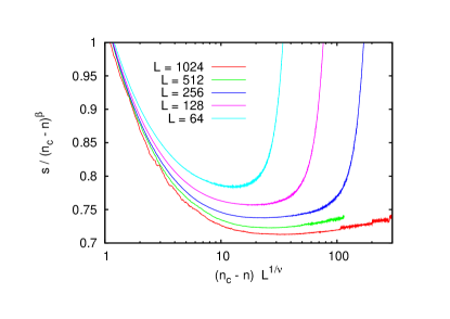
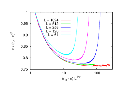
Using the critical exponents for 3-dimensional OP, $\beta=0.4170(3),D_{f}=2.5226(1),$ and $\nu=0.8734(5)$ Deng-2005 , one obtains an acceptable data collapse when plotting $m_{\rm max}/L^{D_{f}}$ against $(n-n_{c})L^{1/\nu}$, with $n_{c}=0.411$. But the behavior for large $L$ is not given by $S\sim(n-n_{c})^{\beta}$ with the value of $\beta$ given above, see Fig. 5. The latter plot is much improved, if we use instead

$$\beta=0.435,\;\;D_{f}=2.522,\;\;\nu=0.91,$$ (5)

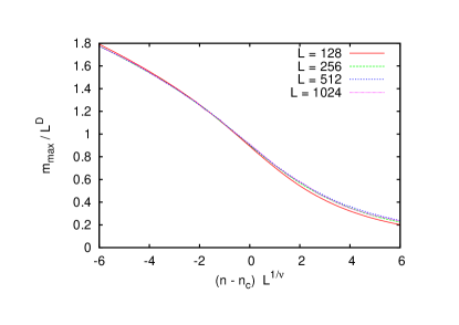
together with $n_{c}=0.4110$ (see Fig. 6). With these exponents we also obtain a good collapse of $m_{\rm max}/L^{D_{f}}$ against $(n-n_{c})L^{1/\nu}$, see Fig. 7. The main deviation from a perfect collapse in this plot is due to the smallest lattice, and is obviously a finite-size correction to the FSS ansatz. We do not quote error bars for the values in Eq.(5), as they are not yet our final estimates.

Figure 5: (Color online) Plot of $S/(n_{c}-n)^{\beta}$ against $(n_{c}-n)L^{1/\nu}$, using the exponents of ordinary 3-d percolation. According to the FSS ansatz, these curves should collapse and should be horizontal in the limit where we first take $L\to\infty$ and then $n\to n_{c}$. This seems not to be the case.

Figure 6: (Color online) Analogous to the previous plot, but using $\beta=0.435,D_{f}=2.5220$, and $\nu=0.91$.

Figure 7: (Color online) Plot of $SL^{\beta/\nu}=m_{\rm max}/L^{D_{f}}$ versus $(n-n_{c})L^{1/\nu}$ for AP on the simple cubic lattice, using $n_{c}=0.411$ and the exponents given in Eq. (5).

IV Bipartivity and Spontaneous symmetry breaking

IV.1 Uniqueness of cluster colors

Our first observation is that infinite square, honeycomb and cubic lattices are bipartite, while the triangular lattice is not. The next observation is that finite square lattices of size $L\times L$ are still bipartite, if $L$ is even and periodic boundary conditions are used, but global bipartivity is lost when either $L$ is odd or helical b.c. are used. These observations strongly suggest that it is indeed bipartivity that is responsible for peculiarities of AP on these lattices.

Figure 8: (Color online) Part of a square lattice with cluster boundaries indicated by black lines. Plaquettes correspond to nodes of the graph. Nine clusters are labeled with letters $A-I$. Six of them ($A,B,D-F$) are single nodes, one ($C$) has five nodes, and two ($H,I$) are very large. Three of them ($D,H,I$) are blue, the other six are white. If cluster $D$ is chosen as target, it merges with $C,E,F$, and $G$ and the new cluster is white. If, however, $F$ is chosen as target, the new blue cluster would consist of $D,H$, and $I$.

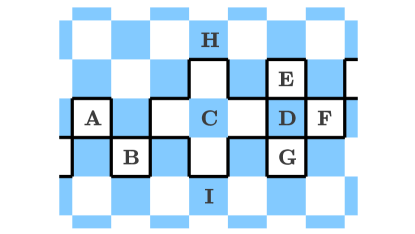
In a bipartite graph, to each node can be assigned one of two colors. We now show that this is extended from single nodes to arbitrarily large clusters, if the rules of AP are strictly followed. Before we do this, we need two definitions:

Definition: The surface of a cluster $C$ is the set of all nodes in $C$ that have at least one link to a node not contained in $C$.

Definition: If all surface nodes in $C$ have the same color, then we say that $C$ also has this color. Otherwise, the color of $C$ is not defined.

We can now prove the following Theorem:
(i) If clusters are grown according to the AP rules on a bipartite network, they always have a well defined color.
(ii) All neighbors of a given cluster have the opposite color.
(iii) If a target of color $c$ is chosen for agglomerating all its neighbors, the new cluster has the opposite color ${\bar{c}}$.

For an illustration see Fig. 8.

Proof: The proof follows by induction. First, the theorem is obviously true for the starting configuration, where all clusters are single nodes. Then, let us assume it is true for all agglomeration steps up to (and including) step $t$. Let us call $c$ the color of the target cluster at step $t+1$, and ${\bar{c}}$ the opposite color. Then all neighbors of the target have color ${\bar{c}}$, so that after joining them the new cluster also has color ${\bar{c}}$, proving thereby (i) and (ii). On the other hand, all neighbors of the neighbors had color $c$, and these form the neighbors of the new cluster, which proves (iii). $\blacksquare$

Notice that it was crucial for the proof that all neighbors of the target were joined, so that none of the neighbors of the target is a neighbor of the new cluster. This shows why imperfect agglomeration as considered in Sec. III.1.2 leads to situations where the theorem does not hold.

IV.2 Coexistence of large clusters

A typical configuration on a $128\times 128$ lattice with three large clusters, none of which has yet wrapped vertically, is shown in Fig. 9. Such a configuration would have an astronomically small probability in OP, since in OP the chance is very small to have more than one large cluster. If there were two large clusters at any time, they would immediately merge with very high probability. Obviously, in AP there exists a mechanism that prevents clusters of opposite color to merge fast, leading to the coexistence of large clusters of opposite colors.

Figure 9: (Color online) A configuration with three large clusters at $n\approx 0.03$ and $L=128$. For clusters of mass $>1$ the two colors are red and blue, with the larger clusters more bright and the smaller ones more dark. “Blue” singletons are colored white for better visibility and in order to distinguish them from “red” singletons which actually are indicated by black squares. Notice that no two clusters of the same color ever touch in this figure. Wherever they seem to touch, there is indeed a small cluster of the opposite color intervening. In spite of the size of the largest clusters, none of them has yet wrapped in the vertical direction.

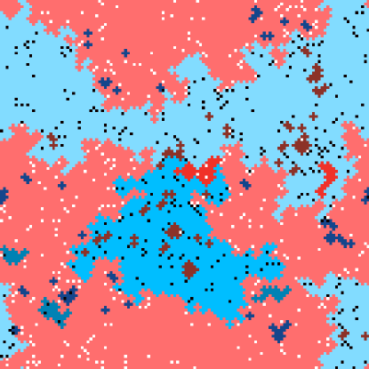
This looks at first paradoxical. Take the two largest clusters in Fig. 9. If either of them were chosen as target, they would merge immediately. Why should this not happen? The crucial point is that each cluster is chosen as target with the same probability, and there are many more small clusters than large ones. The chances are thus overwhelming that neither of the large clusters is chosen as target, but a small cluster is picked instead. But in that case the two largest clusters cannot merge, because they have opposite color and all neighbors to be merged must have the same color. Thus its is most likely that a random agglomeration step merges one small cluster of color $c$ with several (small and large) clusters of color $\bar{c}$.

Figure 10: (Color online) Cluster mass distributions for simple cubic lattices with $L=32$. The curve for $n=0.4323$ is subcritical, while the other curves are supercritical. In contrast to the case of OP, where the mass distribution develops a single peak in the supercritical phase, now (i.e. for AP) we see two peaks. They correspond to clusters of opposite colors.

Figure 11: Average size of the second largest cluster on simple cubic lattices with even size. In contrast to OP, where $m_{\rm max,2}$ peaks near the percolation transition and decreases fast when one goes into the supercritical phase, here the second largest cluster continues to grow far beyond the percolation transition $n_{c}\approx 0.411$.

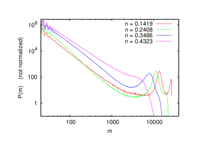
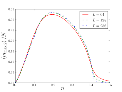
In two dimensions this means also that the two large clusters of opposite color prevent each other from wrapping. In three dimensions this is not the case. Thus AP is in three dimensions more similar to OP, although it still should show several large clusters in the critical and supercritical regimes. To test this prediction we show two figures. Fig. 10 shows that mass distributions in the supercritical phase have two peaks (in contrast to OP), corresponding to the fact that AP on bipartite graphs has two giant clusters of opposite colors. The same conclusion is drawn from Fig. 11, where we show the average normalized size $m_{\rm max,2}$ of the second largest cluster as a function of $n$. We see that $m_{\rm max,2}$ starts to increase at $n_{c}$ and continues to grow as one goes deeper into the supercritical phase, while it would peak at $n_{c}$ in OP.

IV.3 Surface color statistics

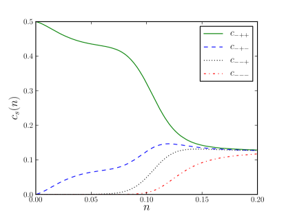
While these two figures show that there is indeed more than one giant cluster in AP on bipartite lattices, they do not yet prove that these clusters have opposite colors. To verify also this prediction we denote the two colors as ‘+’ and ‘$-$’, and define $c_{ijk\ldots}$ ($i,j,k\ldots\in\{+,-\}$) as the probabilities that the largest cluster has color $i$, the second largest $j$, etc. These probabilities are normalized such that $\sum_{ijk\ldots}c_{ijk\ldots}=1$. Due to the symmetry under exchange of colors, $c_{ijk\ldots}=c_{{\bar{i}}{\bar{j}}{\bar{k}}\ldots}$. In Fig. 12 we plot the four probabilities $c_{-jk}$ for square lattices with $L=512$ against $n$. While they are all equal to $\approx 1/8$ for large $n$, this degeneracy is lifted as the agglomeration process proceeds. The most likely color pattern is $(-++)$, followed by $(-+-)$. Both have opposite colors for the two largest clusters. The least likely pattern has all colors the same.

Figure 12: (Color online) Probabilities $c_{s}(n)$ of color patterns $s=(-++),\;(-+-),\;(--+),$ and $(---)$ for the largest three clusters, plotted against $n$. The first index (here always ‘-’) gives the color of the largest cluster, while the other two are for the second and third largest. The data are for square lattices of size $L=512$.

In Fig. 13 we show how the $n$-dependence of the probability $c_{--}$ that the two largest clusters have the same color changes with system size $L$, both for 2 and 3 dimensions. There is a dramatic difference: While the data support our conclusion that there is no transition at any finite $n$ in case of the square lattice (the effective transition point moves to zero as $L$ increases), there is a clear indication for $n_{c}=0.411$ in case of the cubic lattice.

Figure 13: (Color online) Probabilities that the two largest clusters have the same color. According to our theory, these probabilities should vanish in the supercritical phase, if $L\to\infty$. Panel (a) is for the square lattice, panel (b) for the cubic. The upper inset in panel (b) shows the region close to the critical point. The lower inset shows a data collapse plot, $c_{--}(n)$ against $(n-n_{c})L^{1/\nu}$ with $n_{c}=0.4109$ and $\nu=1.01$.

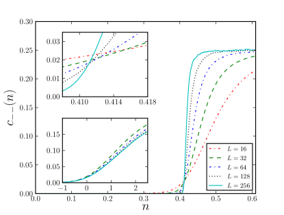
More precisely, the lower inset in Fig. 13 shows a nearly perfect data collapse when plotting $c_{--}(n)$ against $(n-n_{c})L^{1/\nu}$, with $n_{c}=0.4109$ and $\nu=1.01$. The latter values are very close to the values obtained in Sec. III.2.2 from the data collapse for the ordinary order parameter, but sufficiently far from them to call for further, so far unnoticed, corrections to scaling. Combining both sets of parameters, accounting for such corrections by increasing the error estimates, and noticing that the system sizes in Fig. 13 are much smaller than those in Figs. 5 to 7, we get our final result

$$\beta=0.437(6),\;\;D_{f}=2.523(3),\;\;\nu=0.918(13),$$ (6)

and $n_{c}=0.4110(1)$.

Since the differences between these exponents and those of OP are about three to four error bars, we conjecture that the two models are not in the same universality class. But more studies are needed to settle this question beyond reasonable doubts. In any case, Fig. 13 should leave no doubt that $1/4-c_{--}(n)$ is as good an order parameter for the symmetry breaking aspects of the transition, as $S$ is for the percolation aspects.

IV.4 Lattices with local bipartite structure

Let us finally discuss the case where we have locally a bipartite lattice, but where global bipartivity is broken by the boundary conditions. In that case the boundary conditions are irrelevant as long as the cluster does not wrap around the lattice. In particular, we expect that such a system is not in the OP universality class, if the globally bipartite system is not either. More precisely, we expect that clusters of size $<L$ are unaffected by the boundary conditions. Whether critical exponents like the order parameter exponent $\beta$ are affected, which are defined through the behavior of the supercritical phase, is an open question.

V Random bipartite graphs

One minor problem in simulations of random bipartite networks is that we want connected graphs, but the most straightforward way of generating it leads to graphs that are not connected. We thus start with $N^{*}$ nodes, divide them into two equally large groups, and add $zN^{*}/2$ edges which have the two ends in different groups. Here $z$ is the average degree of the entire graph, which is chosen as $z=2$ in the following.

Figure 14: Fraction of nodes in the largest cluster $\left\langle m_{\mathrm{max}}\right\rangle/N$ for random bipartite networks.

Figure 15: Scaling collapse for $\left\langle m_{\mathrm{max}}\right\rangle$ in the critical region for random bipartite networks.

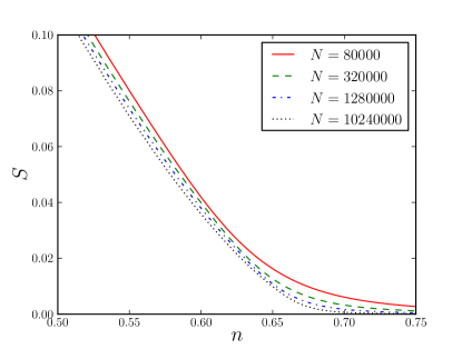
For this value of $z$, the largest connected component of the network constructed this way has $\approx 0.7968N^{*}$ nodes. If we want to have a connected graph with $N$ nodes, we take $N^{*}=N/0.7968$ and discard all those graphs for which the size of the largest connected component is outside the range $N\pm 0.01\%$, and for which any of the two components has size outside the range $N/2\pm 0.01\%$.

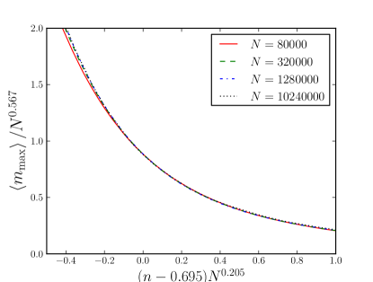
The $n-$dependence of the size of the largest cluster is shown in Fig. 14. We assume again a FSS ansatz analogous to Eq. (4), with $L$ replaced by $N$ (now $D$ can of course not be interpreted as dimension, and $\nu$ no longer is a correlation length exponent). The critical point and the critical exponents are found as (see Fig. 15): $n_{c}=0.695,\;\;\nu=4.88,\;\;D=0.567$.

Figure 16: Probabilities $c_{--}(n)$ for the largest two clusters in a random bipartite network to have the same color, for different system sizes. As also seen from the inset, these curves cross near the estimated critical point $n_{c}\approx 0.696$.

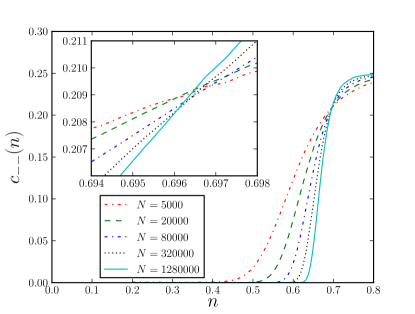
The probabilities $c_{--}(n)$ for both largest cluster to have the same color are shown in Fig. 16. As in the 3-d case (Fig. 13b) we see that the curves for different system sizes cross exactly at the critical point, suggesting again that $c_{--}(n)=0$ in the supercritical phase in the large system limit . We also obtain a perfect data collapse if we plot $c_{--}(n)$ against $(n-n_{c})N^{1/\nu}$, with slightly different parameters $n_{c}=0.696,\;\nu=4.60$ (data not shown). Our best estimates for the critical parameters are the compromise

$$n_{c}=0.695(2),\;\;\nu=4.7(2),\;\;D=0.567(6)\;.$$ (7)

The values for $\nu$ and $D$ are very close to those for Erdös-Renyi networks ($\nu=4.44,\;D=0.60$), although they differ by more than one standard deviation. As in the 3-d case, more work would be needed to determine whether these differences are significant.

VI Generalizations to $k-$partite graphs

A graph is $k-$partite for any $k\geq 2$, if the set of nodes can be divided into $k$ non-empty disjoint subsets ${\cal N}_{m},\;m=1\ldots k$ such that there are no links within any of the ${\cal N}_{m}$. As we saw in Sec. IV, the appearance of novel structures in AP on bipartite graphs depended on the fact that AP does not “mix” colors: After each agglomeration step, one can still associate a unique color to the new cluster. This is no longer true on $k-$partite graphs with $k>2$. Assume a node $i$ has neighbors with two different colors, $c_{1}$ and $c_{2}$ say. Then, if $i$ is chosen as a target, the new cluster will display both colors on its surface.

Figure 17: (Color online) Part of a a triangular lattice where sites (hexagons) are colored red, green and blue. The colors are arranged such that no two sites with the same color are adjacent, i.e. if neighbors are connected by bonds the lattice is tripartite. A modified AP process is defined such that a target with color R can join only with neighbors of color G, G can join only with B, and B can join only with R. This is indicated by the arrows and is denoted by $R\to G\to B\to R$. When node $A$ is chosen as target, it agglomerates with all G neighbors and becomes itself G, so that the new cluster is all G on its surface.

Figure 18: (Color online) Each circle represents a color, i.e. an element of a partition of a $k-$partite network. An arrow from partition $A$ to partition $B$ means that a target with color $A$ joins with all nodes of color $B$. Solid arrows indicate cycles that are followed at each agglomeration step, while dotted arrows indicate random AP rules where different colors are chosen at different time steps.

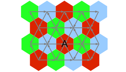
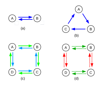
In order to arrive at non-trivial structures we have to generalize the AP rule. Assume we have a $k-$partite graph with colors $c_{1},\ldots c_{k}$. In Fig. 17 we show the triangular lattice as an example of a tripartite graph with colors red (R), green (G) and blue (B). We define then a cycle $\cal C$ in the set of colors as a closed non-intersecting directed path $c_{i_{1}}\to c_{i_{2}}\to\ldots c_{i_{k}}\to c_{i_{1}}$. For tripartite graphs as in Fig. 17 there are two possible cycles, $R\to G\to B\to R$ and $R\to B\to G\to R$ (up to circular shifts). For each cycle $\cal C$ we define a modified AP rule AP_C such that a target with color $c$ joins with all neighbors having the color that follows $c$ in $\cal C$, and only those. After that, the target is recolored to $c$, so that the new cluster has a unique color.

Alternatively, we can define a randomized rule AP_random such that each target node $i$ chooses at random a color $c$ (different from its own) and joins with all neighbors of color $c$. Obviously even more possibilities exist when $k>3$. For instance we can choose the joined neighbors by following some subset of cycles. Different possibilities are illustrated in Fig. 18.

We have not made any simulations, but we expect a rich variety of different behaviors resulting from different rules. It is not clear that in each case AP differs from OP in critical behavior. It is also not clear what happens, if one of the partitions of the network is finite. Naively one should expect that such finite components should not have any influence on critical behavior (which deals only with infinite clusters). But the example of finite $q$ in subsection III.1.2 might suggest otherwise: It could be that even a small number of nodes that do not follow the coloring and AP rules of the majority perturb the evolution sufficiently to change the universality class.

VII Discussion

The main purpose of this paper was to explain in detail the reasons for the dramatic breakdown of universality in agglomerative percolation on 2-d lattices. In finding this reason – and demonstrating numerous other unexpected features of AP in these cases – we indeed uncovered a new class of models with non-trivial symmetries. In the present paper only the simplest of these, having a $Z_{2}$ symmetry due to bipartivity, is treated in detail, while more complex situations leading to higher symmetries are only sketched.

Agglomerative percolation is a very natural extension of the standard percolation model, and we expect a number of applications (some of which were already mentioned in Christen-2010 ). The main effect of bipartivity in AP is that the merging of large clusters is delayed, as compared to OP. It shares this feature with explosive percolation Achli-2009 , but in contrast to the latter this delay is not imposed artificially, but is a natural consequence of the structure of the model. Also, the merging of large clusters is not delayed in all circumstances, but only subject to the symmetry structure imposed by bipartivity. The latter implies that clusters can have “colors” (with $k$ colors in case of a $k-$partite network), and only the merging of clusters with different colors is delayed.

The effect of bipartivity is dramatic in case of 2-d lattices – shifting, in particular, the percolation threshold on infinite systems to the limit where the average cluster size diverges and the number of clusters per site is zero. It is much less dramatic for 3-d lattices (where we studied only the simple cubic lattice) and for random networks. In these cases we see a clear effect, and the simulations indicate that universality with OP is broken, but the percolation threshold is at finite values and the critical exponents are close to those of OP.

Future work is needed to settle these questions of universality. In particular, it would be of interest to study high-dimensional ($3<d\leq 6$) simple hypercubic lattices, in order to see how the lattice models cross over to the random graph model. Another interesting subject for future work is a modified AP model (discussed briefly in Sec. VI) on the triangular lattice, where the relevant group is $Z_{3}$ instead of $Z_{2}$. Finally, there should exist a rich mathematical structure for modified AP models on $k-$partite networks with $k>3$, all of which is not yet understood.

References

- (1) D. S. Callaway, M. E. J. Newman, S. H. Strogatz, and D. J. Watts, Phys. Rev. Lett. 85, 5468 (2000)
- (2) D. Achlioptas, R. M. D’Souza, and J. Spencer, Science 323, 1453 (2009)
- (3) R. A. da Costa, S. N. Dogorovtsev, A. V. Goltsev, and J. F. F. Mendes, Phys. Rev. Lett. 105, 255701 (2010)
- (4) O. Riordan and L. Warnke, Science 333, 322 (2011)
- (5) P. Grassberger, C. Christensen, G. Bizhani, S.-W. Son, and M. Paczuski, Phys. Rev. Lett. 106, 225701 (2011)
- (6) S. V. Buldyrev, R. Parshani, G. Paul, H. E. Stanley, and S. Havlin, Nature 464, 1025 (2010)
- (7) R. Parshani, S. V. Buldyrev, and S. Havlin, Phys. Rev. Lett. 105, 048701 (2010)
- (8) S.-W. Son, G. Bizhani, C. Christensen, P. Grassberger, and M. Paczuski, Europhys. Lett. 97, 16006 (2012)
- (9) S.-W. Son, P. Grassberger, and M. Paczuski, Phys. Rev. Lett. 107, 195702 (2011)
- (10) C. Song, S. Havlin, and H. A. Makse, Nature 433, 392 (2004)
- (11) F. Radicchi, A. Barrat, S. Fortunato, and J. Ramasco, Phys. Rev. E 79, 026104 (2009)
- (12) G. Bizhani, V. Sood, M. Paczuski, and P. Grassberger, Phys. Rev. E 83, 036110 (2011)
- (13) C. Christensen, G. Bizhani, S.-W. Son, M. Paczuski, and P. Grassberger, Europhys. Lett. 97, 16004 (2012)
- (14) S.-W. Son, C. Christensen, G. Bizhani, P. Grassberger, and M. Paczuski, Phys. Rev. E 84, 040102(R) (2011)
- (15) S.-W. Son, G. Bizhani, C. Christensen, P. Grassberger, and M. Paczuski, Europhys. Lett. 95, 58007 (2011)
- (16) G. Bizhani, P. Grassberger, and M. Paczuski, Phys. Rev. E 84, 066111 (2011)
- (17) D. Stauffer and A. Aharony, Introduction to Percolation Theory (Taylor & Francis, London, 1994)
- (18) S. Boettcher, V. Singh, and R. M. Ziff, arXiv:1110.4288(2011)
- (19) M. E. J. Newman and R. M. Ziff, Phys. Rev. E 64, 016706 (2001)
- (20) R. M. Ziff, Phys. Rev. Lett. 103, 045701 (2009)
- (21) Y. Deng and H. W. J. Blöte, Phys. Rev. E 72, 016126 (2005)
- (22) For very small and very large , is ill defined, because in these limits there can be more than one largest (or second largest) cluster, but this affects only regions infinitesimally close to and in the limit .