A strategy towards the extraction of the Sivers function with TMD evolution

M. Anselmino Dipartimento di Fisica Teorica, Università di Torino, Via P. Giuria 1, I-10125 Torino, Italy INFN, Sezione di Torino, Via P. Giuria 1, I-10125 Torino, Italy    M. Boglione Dipartimento di Fisica Teorica, Università di Torino, Via P. Giuria 1, I-10125 Torino, Italy INFN, Sezione di Torino, Via P. Giuria 1, I-10125 Torino, Italy    S. Melis European Centre for Theoretical Studies in Nuclear Physics and Related Areas (ECT*),
Villa Tambosi, Strada delle Tabarelle 286, I-38123 Villazzano, Trento, Italy
Abstract

The QCD evolution of the unpolarized Transverse Momentum Dependent (TMD) distribution functions and of the Sivers functions have been discussed in recent papers. Following such results we reconsider previous extractions of the Sivers functions from semi-inclusive deep inelastic scattering data and propose a simple strategy which allows to take into account the Q2superscript𝑄2Q^{2} dependence of the TMDs in comparison with experimental findings. A clear evidence of the phenomenological success of the TMD evolution equations is given, mostly, by the newest COMPASS data off a transversely polarized proton target.

pacs:
13.88.+e, 13.60.-r, 13.85.Ni

I Introduction and formalism

The exploration of the 3-dimensional structure of the nucleons, both in momentum and configuration space, is one of the major issues in hadron high energy physics, with dedicated experimental and theoretical efforts. In particular, several Semi-Inclusive Deep Inelastic Scattering (SIDIS) experiments are either running or being planned. From the measurements of azimuthal asymmetries, both with unpolarized and polarized nucleons, one obtains information on the Transverse Momentum Dependent Parton Distribution Functions (TMD PDFs) and on the Transverse Momentum Dependent Fragmentation Functions (TMD FFs). The TMD PDFs and the TMD FFs are often globally referred to simply as TMDs. The TMD PDFs convey information on the momentum distributions of partons inside protons and neutrons.

The analysis of the experimental data is based on the so-called TMD factorization, which links measurable cross sections and spin asymmetries to a convolution of TMDs. In particular, the Sivers function, which describes the number density of unpolarized quarks inside a transversely polarized proton, has received much attention and has been extracted from SIDIS data by several groups, with consistent results Anselmino:2005ea ; Collins:2005ie ; Vogelsang:2005cs ; Anselmino:2005an ; Anselmino:2008sga ; Bacchetta:2011gx . However, all these phenomenological fits of the Sivers function (and other TMDs) have been performed so far using a simplified version of the TMD factorization scheme, in which the QCD scale dependence of the TMDs – which was unknown – is either neglected or limited to the collinear part of the unpolarized PDFs. While this might not be a serious numerical problem when considering only experimental data which cover limited ranges of low Q2superscript𝑄2Q^{2} values, it is not correct in principle, and taking into account the appropriate Q2superscript𝑄2Q^{2} evolution might be numerically relevant for predictions at higher Q2superscript𝑄2Q^{2} values, like future electron-ion or electron-nucleon colliders (EIC/ENC) and Drell-Yan experiments.

Recently, the issue of the QCD evolution of unpolarized TMDs and of the Sivers function has been studied in a series of papers Collins:2011book ; Aybat:2011zv ; Aybat:2011ge and a complete TMD factorization framework is now available for a consistent treatment of SIDIS data and the extraction of TMDs. A first application of the new TMD evolution equations to some limited samples of the HERMES and COMPASS data Aybat:2011ta has indeed shown clear signs of the Q2superscript𝑄2Q^{2} TMD evolution.

We follow here Refs. Aybat:2011zv and Aybat:2011ge adopting their formalism, which includes the explicit Q2superscript𝑄2Q^{2} dependence of the TMDs, and apply it to the extraction of the Sivers function from SIDIS data, exploiting the latest HERMES :2009ti and COMPASS Bradamante:2011xu results. In the sequel of this Section we present the explicit formalism: in Subsection I.1 we describe the setup and structure of the TMD evolution equations, in Subsection I.2 we discuss the parameterizations used for the unknown input functions, while in Subsection I.3 we present analytical solutions of the TMD evolutions equations obtained under a specific approximation.

In Section II we perform a best fit of the SIDIS Sivers asymmetries taking into account the different Q2superscript𝑄2Q^{2} values of each data point and the Q2superscript𝑄2Q^{2} dependence of the TMDs; we compare our results with a similar analysis performed without the TMD evolution. Differences between Sivers functions extracted from data with and without the TMD evolution are shown and commented. In all this we differ from Ref. Aybat:2011ta , which explicitly shows the evolution of an existing fit of the Sivers SIDIS asymmetry Anselmino:2011gs from the average value Q2=2.4delimited-⟨⟩superscript𝑄22.4\langle Q^{2}\rangle=2.4 GeV2 for HERMES data :2009ti to the average value of Q2=3.8delimited-⟨⟩superscript𝑄23.8\langle Q^{2}\rangle=3.8 GeV2 for the most recent COMPASS data Bradamante:2011xu . Further comments and conclusions are given in Section III.

I.1 Formalism for TMD Q2superscript𝑄2Q^{2} dependence

In Refs. Collins:2011book and Aybat:2011zv , Collins, Aybat and Rogers have proposed a scheme to describe the Q2superscript𝑄2Q^{2} evolution of the TMD unpolarized distribution and fragmentation functions: within the framework of the Collins-Soper-Sterman (CSS) factorization formalism Collins:1981va ; Collins:1984kg , they can describe the non-perturbative, low transverse momentum region and, at the same time, consistently include the perturbative corrections affecting the region of larger energies and momentum transfers. However, this formalism cannot be directly applied to spin dependent distribution functions, like the Sivers function Sivers:1989cc , for which the collinear limit does not exist.

More recently, an extension of the unpolarized TMD-evolution formalism was presented in Ref. Aybat:2011ge to provide a framework in which also spin-correlated PDFs can be accounted for. For our purposes, we will use Eq. (44) of Ref. Aybat:2011ge which, compared to the unpolarized TMD evolution scheme, Eq. (26) of Ref. Aybat:2011zv , requires the extra aid of a phenomenological input function embedding the missing information on the evolved function, that, in the case of the Sivers function, is both of perturbative and non-pertubative nature. Although the unpolarized PDF and FF TMD evolution equations are in principle known Aybat:2011zv , in this paper we adopt the simplified functional form of the evolution equation, as proposed for the Sivers function in Ref. Aybat:2011ge , for all TMD functions, for consistency.

Thus, we strictly follow Ref. Aybat:2011ge and combine their Eqs. (44), (43) and (30), taking, as suggested Aybat:2011ge , the renormalization scale μ2superscript𝜇2\mu^{2} and the regulating parameters ζFsubscript𝜁𝐹\zeta_{F} and ζDsubscript𝜁𝐷\zeta_{D} all equal to Q2superscript𝑄2Q^{2}. Then, the QCD evolution of the TMDs in the coordinate space can be written as

F~(x,𝒃T;Q)=F~(x,𝒃T;Q0)exp{lnQQ0K~(bT;Q0)+Q0QdμμγF(μ,Q2μ2)},~𝐹𝑥subscript𝒃𝑇𝑄~𝐹𝑥subscript𝒃𝑇subscript𝑄0𝑄subscript𝑄0~𝐾subscript𝑏𝑇subscript𝑄0superscriptsubscriptsubscript𝑄0𝑄d𝜇𝜇subscript𝛾𝐹𝜇superscript𝑄2superscript𝜇2\widetilde{F}(x,\mbox{\boldmath$b$}_{T};Q)=\widetilde{F}(x,\mbox{\boldmath$b$}_{T};Q_{0})\exp\left\{\ln\frac{Q}{Q_{0}}\>\widetilde{K}(b_{T};Q_{0})+\int_{Q_{0}}^{Q}\frac{\rm d\mu}{\mu}\gamma_{F}\left(\mu,\frac{Q^{2}}{\mu^{2}}\right)\right\}\>, (1)

where F~~𝐹\widetilde{F} can be either the unpolarized parton distribution, F~(x,𝒃T;Q)=f~q/p(x,𝒃T;Q)~𝐹𝑥subscript𝒃𝑇𝑄subscript~𝑓𝑞𝑝𝑥subscript𝒃𝑇𝑄\widetilde{F}(x,\mbox{\boldmath$b$}_{T};Q)=\widetilde{f}_{q/p}(x,\mbox{\boldmath$b$}_{T};Q), the unpolarized fragmentation function F~(x,𝒃T;Q)=D~h/q(z,𝒃T;Q)~𝐹𝑥subscript𝒃𝑇𝑄subscript~𝐷𝑞𝑧subscript𝒃𝑇𝑄\widetilde{F}(x,\mbox{\boldmath$b$}_{T};Q)=\widetilde{D}_{h/q}(z,\mbox{\boldmath$b$}_{T};Q), or the first derivative, with respect to the parton impact parameter bTsubscript𝑏𝑇b_{T}, of the Sivers function, F~(x,𝒃T;Q)=f~1Tf(x,𝒃T;Q)~𝐹𝑥subscript𝒃𝑇𝑄superscriptsubscript~𝑓1𝑇perpendicular-toabsent𝑓𝑥subscript𝒃𝑇𝑄\widetilde{F}(x,\mbox{\boldmath$b$}_{T};Q)=\widetilde{f}_{1T}^{\prime\perp f}(x,\mbox{\boldmath$b$}_{T};Q). Notice that throughout the paper bTsubscript𝑏𝑇b_{T}-dependent distribution and fragmentation functions will be denoted with a similar-to\sim on top.

In the above equation the function K~~𝐾\widetilde{K} is given in general by Aybat:2011ge :

K~(bT,μ)=K~(b,μb)+[μμbdμμγK(μ)]gK(bT),~𝐾subscript𝑏𝑇𝜇~𝐾subscript𝑏subscript𝜇𝑏delimited-[]superscriptsubscript𝜇subscript𝜇𝑏dsuperscript𝜇superscript𝜇subscript𝛾𝐾superscript𝜇subscript𝑔𝐾subscript𝑏𝑇\widetilde{K}(b_{T},\mu)=\widetilde{K}(b_{*},\mu_{b})+\left[\int_{\mu}^{\mu_{b}}\frac{\rm d\mu^{\prime}}{\mu^{\prime}}\gamma_{K}(\mu^{\prime})\right]-g_{K}(b_{T})\>, (2)

with, at 𝒪(αs)𝒪subscript𝛼𝑠{\cal O}(\alpha_{s}) Collins:1981va ; Collins:1984kg ,

K~(b,μb)=αsCFπ[ln(b2μb2)ln4+2γE]~𝐾subscript𝑏subscript𝜇𝑏subscript𝛼𝑠subscript𝐶𝐹𝜋delimited-[]superscriptsubscript𝑏2superscriptsubscript𝜇𝑏242subscript𝛾𝐸\widetilde{K}(b_{*},\mu_{b})=-\frac{\alpha_{s}\,C_{F}}{\pi}\left[\ln(b_{*}^{2}\,\mu_{b}^{2})-\ln 4+2\gamma_{E}\right] (3)
b(bT)bT1+bT2/bmax2μb=C1b(bT)b_{*}(b_{T})\equiv\frac{b_{T}}{\sqrt{1+b_{T}^{2}/b_{\rm max}^{2}}}\quad\quad\quad\mu_{b}=\frac{C_{1}}{b_{*}(b_{T})}\>\cdot (4)

The first two terms in Eq. (2) are perturbative and depend on the scale μ𝜇\mu through the coupling αs(μ)subscript𝛼𝑠𝜇\alpha_{s}(\mu), while the last term is non-perturbative, but scale independent. C1subscript𝐶1C_{1} is a constant parameter which can be fixed to optimize the perturbative expansion, as explained in Ref. Collins:1984kg . Refs. Aybat:2011zv and Aybat:2011ge adopt the particular choice C1=2eγEsubscript𝐶12superscript𝑒subscript𝛾𝐸C_{1}=2e^{-\gamma_{E}} which automatically implies K~(b,μb)=0~𝐾subscript𝑏subscript𝜇𝑏0\widetilde{K}(b_{*},\mu_{b})=0, considerably simplifying the bTsubscript𝑏𝑇b_{T} dependence of the CSS kernel K~(bT,μ)~𝐾subscript𝑏𝑇𝜇\widetilde{K}(b_{T},\mu), Eq. (2).

The anomalous dimensions γFsubscript𝛾𝐹\gamma_{F} and γKsubscript𝛾𝐾\gamma_{K} appearing respectively in Eqs. (1) and (2), are given, again at order 𝒪(αs)𝒪subscript𝛼𝑠{\cal O}(\alpha_{s}), by Collins:1984kg ; Aybat:2011zv

γF(μ;Q2μ2)=αs(μ)CFπ(32lnQ2μ2)γK(μ)=αs(μ)2CFπ\gamma_{F}(\mu;\frac{Q^{2}}{\mu^{2}})=\alpha_{s}(\mu)\,\frac{C_{F}}{\pi}\left(\frac{3}{2}-\ln\frac{Q^{2}}{\mu^{2}}\right)\quad\quad\quad\quad\gamma_{K}(\mu)=\alpha_{s}(\mu)\,\frac{2\,C_{F}}{\pi}\>\cdot (5)

By making use of Eqs. (2)-(5), the evolution of F~(x,𝒃T;Q)~𝐹𝑥subscript𝒃𝑇𝑄\widetilde{F}(x,\mbox{\boldmath$b$}_{T};Q) in Eq. (1) can then be written as:

F~(x,𝒃T;Q)=F~(x,𝒃T;Q0)R~(Q,Q0,bT)exp{gK(bT)lnQQ0},~𝐹𝑥subscript𝒃𝑇𝑄~𝐹𝑥subscript𝒃𝑇subscript𝑄0~𝑅𝑄subscript𝑄0subscript𝑏𝑇subscript𝑔𝐾subscript𝑏𝑇𝑄subscript𝑄0\widetilde{F}(x,\mbox{\boldmath$b$}_{T};Q)=\widetilde{F}(x,\mbox{\boldmath$b$}_{T};Q_{0})\>\widetilde{R}(Q,Q_{0},b_{T})\>\exp\left\{-g_{K}(b_{T})\ln\frac{Q}{Q_{0}}\right\}\>, (6)

with

R~(Q,Q0,bT)exp{lnQQ0Q0μbdμμγK(μ)+Q0QdμμγF(μ,Q2μ2)}\widetilde{R}(Q,Q_{0},b_{T})\equiv\exp\left\{\ln\frac{Q}{Q_{0}}\int_{Q_{0}}^{\mu_{b}}\frac{\rm d\mu^{\prime}}{\mu^{\prime}}\gamma_{K}(\mu^{\prime})+\int_{Q_{0}}^{Q}\frac{\rm d\mu}{\mu}\gamma_{F}\left(\mu,\frac{Q^{2}}{\mu^{2}}\right)\right\}\>\cdot (7)

The Q2superscript𝑄2Q^{2} evolution is driven by the functions gK(bT)subscript𝑔𝐾subscript𝑏𝑇g_{K}(b_{T}) and R~(Q,Q0,bT)~𝑅𝑄subscript𝑄0subscript𝑏𝑇\widetilde{R}(Q,Q_{0},b_{T}). While the latter, Eq. (7), can be easily evaluated, numerically or even analytically, the former, is essentially unknown and will need to be taken from independent experimental inputs.

The explicit expression of the TMDs in the momentum space, with the QCD Q2superscript𝑄2Q^{2} dependence, can be obtained by Fourier-transforming Eq. (6), obtaining Aybat:2011ge :

f^q/p(x,k;Q)=12π0dbTbTJ0(kbT)f~q/p(x,bT;Q)subscript^𝑓𝑞𝑝𝑥subscript𝑘perpendicular-to𝑄12𝜋superscriptsubscript0differential-dsubscript𝑏𝑇subscript𝑏𝑇subscript𝐽0subscript𝑘perpendicular-tosubscript𝑏𝑇subscript~𝑓𝑞𝑝𝑥subscript𝑏𝑇𝑄\widehat{f}_{q/p}(x,k_{\perp};Q)=\frac{1}{2\pi}\int_{0}^{\infty}\!\!\!{\rm d}b_{T}\>b_{T}\>J_{0}(k_{\perp}b_{T})\>\widetilde{f}_{q/p}(x,b_{T};Q) (8)
D^h/q(z,p;Q)=12π0dbTbTJ0(kTbT)D~h/q(z,bT;Q)subscript^𝐷𝑞𝑧subscript𝑝perpendicular-to𝑄12𝜋superscriptsubscript0differential-dsubscript𝑏𝑇subscript𝑏𝑇subscript𝐽0subscriptk𝑇subscript𝑏𝑇subscript~𝐷𝑞𝑧subscript𝑏𝑇𝑄\widehat{D}_{h/q}(z,p_{\perp};Q)=\frac{1}{2\pi}\int_{0}^{\infty}\!\!\!{\rm d}b_{T}\>b_{T}\>J_{0}({\rm k}_{T}b_{T})\>\widetilde{D}_{h/q}(z,b_{T};Q) (9)
f^1Tf(x,k;Q)=12πk0dbTbTJ1(kbT)f~1Tq(x,bT;Q),superscriptsubscript^𝑓1𝑇perpendicular-toabsent𝑓𝑥subscript𝑘perpendicular-to𝑄12𝜋subscript𝑘perpendicular-tosuperscriptsubscript0differential-dsubscript𝑏𝑇subscript𝑏𝑇subscript𝐽1subscript𝑘perpendicular-tosubscript𝑏𝑇superscriptsubscript~𝑓1𝑇perpendicular-toabsent𝑞𝑥subscript𝑏𝑇𝑄\widehat{f}_{1T}^{\perp f}(x,k_{\perp};Q)=\frac{-1}{2\pi k_{\perp}}\int_{0}^{\infty}\!\!\!{\rm d}b_{T}\>b_{T}\>J_{1}(k_{\perp}b_{T})\>\widetilde{f}_{1T}^{\prime\,\perp q}(x,b_{T};Q)\>, (10)

where J0subscript𝐽0J_{0} and J1subscript𝐽1J_{1} are Bessel functions. In this paper we denote the distribution and fragmentation functions which depend on the transverse momenta (TMDs) with a “widehat” on top. f^q/psubscript^𝑓𝑞𝑝\widehat{f}_{q/p} is the unpolarized TMD distribution function for a parton of flavor q𝑞q inside a proton, and D^h/qsubscript^𝐷𝑞\widehat{D}_{h/q} is the unpolarized TMD fragmentation function for hadron hh inside a parton q𝑞q. f^1Tqsuperscriptsubscript^𝑓1𝑇perpendicular-toabsent𝑞\widehat{f}_{1T}^{\perp q} is the Sivers distribution defined, for unpolarized partons inside a transversely polarized proton, as:

f^q/p(x,𝒌,𝑺;Q)subscript^𝑓𝑞superscript𝑝𝑥subscript𝒌perpendicular-to𝑺𝑄\displaystyle\widehat{f}_{q/p^{\uparrow}}(x,\mbox{\boldmath$k$}_{\perp},\mbox{\boldmath$S$};Q) =\displaystyle= f^q/p(x,k;Q)f^1Tq(x,k;Q)ϵijkiSjMpsubscript^𝑓𝑞𝑝𝑥subscript𝑘perpendicular-to𝑄superscriptsubscript^𝑓1𝑇perpendicular-toabsent𝑞𝑥subscript𝑘perpendicular-to𝑄subscriptitalic-ϵ𝑖𝑗superscriptsubscript𝑘perpendicular-to𝑖superscript𝑆𝑗subscript𝑀𝑝\displaystyle\widehat{f}_{q/p}(x,k_{\perp};Q)-\widehat{f}_{1T}^{\perp q}(x,k_{\perp};Q)\frac{\epsilon_{ij}\,k_{\perp}^{i}\,S^{j}}{M_{p}} (11)
=\displaystyle= f^q/p(x,k;Q)+12ΔNf^q/p(x,k;Q)ϵijkiSjk\displaystyle\widehat{f}_{q/p}(x,k_{\perp};Q)+\frac{1}{2}\Delta^{N}\widehat{f}_{q/p^{\uparrow}}(x,k_{\perp};Q)\frac{\epsilon_{ij}\,k_{\perp}^{i}\,S^{j}}{k_{\perp}}\>\cdot (12)

In our notation 𝒌subscript𝒌perpendicular-to\mbox{\boldmath$k$}_{\perp} is the transverse momentum of the parton with respect to the parent nucleon direction and 𝒑subscript𝒑perpendicular-to\mbox{\boldmath$p$}_{\perp} is the transverse momentum of the final hadron with respect to the parent parton direction. Notice that in Refs. Aybat:2011zv and Aybat:2011ge all transverse momenta are defined in a unique frame, the so-called hadron frame, in which the measured hadrons have zero transverse momentum. In this frame, the initial and the final parton transverse momenta are denoted, respectively, by 𝐤1Tsubscript𝐤1𝑇{\bf k}_{1T} and 𝐤2Tsubscript𝐤2𝑇{\bf k}_{2T}. They are related to our notation by: 𝒌=𝐤1Tsubscript𝒌perpendicular-tosubscript𝐤1𝑇\mbox{\boldmath$k$}_{\perp}={\bf k}_{1T} and, at leading order in psubscript𝑝perpendicular-top_{\perp}, 𝒑=z𝐤2Tsubscript𝒑perpendicular-to𝑧subscript𝐤2𝑇\mbox{\boldmath$p$}_{\perp}=-z\,{\bf k}_{2T}. This requires some attention when dealing with the fragmentation functions. Usually, the TMD FFs are defined in terms of the hadronic psubscript𝑝perpendicular-top_{\perp}, i.e. the transverse momentum of the final hadron hh with respect to the direction of the fragmenting parton q𝑞q, while, following Refs. Aybat:2011zv and Aybat:2011ge , the Fourier transform (9) is performed from the impact parameter space of the fragmenting parton (bTsubscript𝑏𝑇b_{T}) into the corresponding partonic transverse momentum (k=Tp/z{}_{T}=p_{\perp}/z) in the hadron frame. This will generate some extra z2superscript𝑧2z^{2} factors, as explained in detail in Section I.2.

I.2 Parameterization of unknown functions

Eqs. (8)-(10) can be adopted as the appropriate functional forms, with the correct Q2superscript𝑄2Q^{2} dependence induced by Eqs. (6)-(7), to be used in the extraction of phenomenological information on the unpolarized and Sivers TMDs. In order to do so, one should start with a parameterization of the unknown functions inside Eq. (6): gK(bT)subscript𝑔𝐾subscript𝑏𝑇g_{K}(b_{T}) and F~(x,bT;Q0)~𝐹𝑥subscript𝑏𝑇subscript𝑄0\widetilde{F}(x,b_{T};Q_{0}). As already anticipated, gK(bT)subscript𝑔𝐾subscript𝑏𝑇g_{K}(b_{T}) is a non-perturbative, but universal function, which in the literature is usually parameterized in a quadratic form. As in Refs. Aybat:2011ge and Aybat:2011ta , we will adopt the results provided by a recent fit of Drell-Yan data Landry:2002ix , and assume

gK(bT)=12g2bT2withg2=0.68correspondingtobmax=0.5GeV1.formulae-sequencesubscript𝑔𝐾subscript𝑏𝑇12subscript𝑔2superscriptsubscript𝑏𝑇2withformulae-sequencesubscript𝑔20.68correspondingtosubscript𝑏max0.5superscriptGeV1g_{K}(b_{T})=\frac{1}{2}\,g_{2}\,b_{T}^{2}\quad\quad{\rm with}\quad\quad g_{2}=0.68\quad\quad{\rm corresponding~{}to}\quad\quad b_{\rm max}=0.5\>{\rm GeV}^{-1}\>. (13)

We should now parameterize the function F~(x,bT;Q0)~𝐹𝑥subscript𝑏𝑇subscript𝑄0\widetilde{F}(x,b_{T};Q_{0}) in configuration space. We wish to test the effect of the TMD evolution in the extraction of the Sivers functions from data; in particular we will compare the extraction based on TMD evolution with previous extractions which did not take such an evolution into account. Then, we parameterize the input function F~(x,bT;Q0)~𝐹𝑥subscript𝑏𝑇subscript𝑄0\widetilde{F}(x,b_{T};Q_{0}) by requiring that its Fourier-transform, which gives the corresponding TMD function in the transverse momentum space, coincides with the previously adopted ksubscript𝑘perpendicular-tok_{\perp}-Gaussian form, with the x𝑥x dependence factorized out. That was also done in Refs. Aybat:2011zv and Aybat:2011ge , assuming for the unpolarized TMD PDF

f~q/p(x,bT;Q0)=fq/p(x,Q0)exp{α2bT2},subscript~𝑓𝑞𝑝𝑥subscript𝑏𝑇subscript𝑄0subscript𝑓𝑞𝑝𝑥subscript𝑄0superscript𝛼2superscriptsubscript𝑏𝑇2\widetilde{f}_{q/p}(x,b_{T};Q_{0})=f_{q/p}(x,Q_{0})\exp\left\{-\alpha^{2}\,b_{T}^{2}\right\}\>, (14)

where fq/p(x,Q0)subscript𝑓𝑞𝑝𝑥subscript𝑄0f_{q/p}(x,Q_{0}) is the usual integrated PDF of parton q𝑞q inside proton p𝑝p, evaluated at Q0subscript𝑄0Q_{0}; the value of α2superscript𝛼2\alpha^{2} is fixed by requiring the desired behavior of the distribution function in the transverse momentum space at the initial scale Q0subscript𝑄0Q_{0}: taking α2=k2/4superscript𝛼2delimited-⟨⟩superscriptsubscript𝑘perpendicular-to24\alpha^{2}=\langle k_{\perp}^{2}\rangle/4 one recovers

f^q/p(x,k;Q0)=fq/p(x,Q0)1πk2ek2/k2,subscript^𝑓𝑞𝑝𝑥subscript𝑘perpendicular-tosubscript𝑄0subscript𝑓𝑞𝑝𝑥subscript𝑄01𝜋delimited-⟨⟩superscriptsubscript𝑘perpendicular-to2superscript𝑒superscriptsubscript𝑘perpendicular-to2delimited-⟨⟩superscriptsubscript𝑘perpendicular-to2\widehat{f}_{q/p}(x,k_{\perp};Q_{0})=f_{q/p}(x,Q_{0})\,\frac{1}{\pi\langle k_{\perp}^{2}\rangle}\,e^{-{k_{\perp}^{2}}/{\langle k_{\perp}^{2}\rangle}}\,, (15)

in agreement with Refs. Anselmino:2008sga ; Anselmino:2011gs ; Anselmino:2011ch .

Similar relations hold for the TMD FFs, with an additional z2superscript𝑧2z^{2} factor due to the fact that the Fourier-transform (9) leads from the impact parameter space of the fragmenting parton in the hadron frame to the corresponding partonic transverse momentum kT, while the TMD FFs are functions of the transverse momentum p=zkTsubscript𝑝perpendicular-to𝑧subscriptk𝑇p_{\perp}=z\,{\rm k}_{T} of the final hadron with respect to the fragmenting parton direction. This requires the initial parameterization

D~h/q(z,bT;Q0)=1z2Dh/q(z,Q0)exp{β2bT2},subscript~𝐷𝑞𝑧subscript𝑏𝑇subscript𝑄01superscript𝑧2subscript𝐷𝑞𝑧subscript𝑄0superscript𝛽2superscriptsubscript𝑏𝑇2\widetilde{D}_{h/q}(z,b_{T};Q_{0})=\frac{1}{z^{2}}\,D_{h/q}(z,Q_{0})\;\exp\left\{-\beta^{2}\,b_{T}^{2}\right\}\>, (16)

where Dh/q(z,Q0)subscript𝐷𝑞𝑧subscript𝑄0D_{h/q}(z,Q_{0}) is the usual integrated FF evaluated at the initial scale Q0subscript𝑄0Q_{0}, and β2=p2/4z2superscript𝛽2delimited-⟨⟩superscriptsubscript𝑝perpendicular-to24superscript𝑧2\beta^{2}=\langle p_{\perp}^{2}\rangle/4z^{2} in order to recover the previously adopted behavior Anselmino:2008sga ; Anselmino:2011gs ; Anselmino:2011ch of the fragmentation function in the psubscript𝑝perpendicular-top_{\perp} transverse momentum space at Q0subscript𝑄0Q_{0}:

D^h/q(z,p;Q0)=Dh/q(z,Q0)1πp2ep2/p2.subscript^𝐷𝑞𝑧subscript𝑝perpendicular-tosubscript𝑄0subscript𝐷𝑞𝑧subscript𝑄01𝜋delimited-⟨⟩superscriptsubscript𝑝perpendicular-to2superscript𝑒superscriptsubscript𝑝perpendicular-to2delimited-⟨⟩superscriptsubscript𝑝perpendicular-to2\widehat{D}_{h/q}(z,p_{\perp};Q_{0})=D_{h/q}(z,Q_{0})\,\frac{1}{\pi\langle p_{\perp}^{2}\rangle}\,e^{-p_{\perp}^{2}/\langle p_{\perp}^{2}\rangle}\>. (17)

Analogously, we parameterize the Sivers function at the initial scale Q0subscript𝑄0Q_{0} as

f~1T(x,bT;Q0)=2γ2f1T(x;Q0)bTeγ2bT2,superscriptsubscript~𝑓1𝑇perpendicular-to𝑥subscript𝑏𝑇subscript𝑄02superscript𝛾2superscriptsubscript𝑓1𝑇perpendicular-to𝑥subscript𝑄0subscript𝑏𝑇superscript𝑒superscript𝛾2superscriptsubscript𝑏𝑇2\widetilde{f}_{1T}^{\prime\perp}(x,b_{T};Q_{0})=-2\,\gamma^{2}\,f_{1T}^{\perp}(x;Q_{0})\,b_{T}\,e^{-\gamma^{2}\,b_{T}^{2}}\>, (18)

which, when Fourier-transformed according to Eq. (10), yields:

f^1T(x,k;Q0)=f1T(x;Q0)14πγ2ek2/4γ2.superscriptsubscript^𝑓1𝑇perpendicular-to𝑥subscript𝑘perpendicular-tosubscript𝑄0superscriptsubscript𝑓1𝑇perpendicular-to𝑥subscript𝑄014𝜋superscript𝛾2superscript𝑒superscriptsubscript𝑘perpendicular-to24superscript𝛾2\widehat{f}_{1T}^{\perp}(x,k_{\perp};Q_{0})=f_{1T}^{\perp}(x;Q_{0})\,\frac{1}{4\,\pi\,\gamma^{2}}\,e^{-k_{\perp}^{2}/4\gamma^{2}}\>. (19)

Eq. (19) agrees with our previous parameterization of the Sivers function, at the initial scale Q0subscript𝑄0Q_{0} Anselmino:2008sga ; Anselmino:2011gs ; Anselmino:2011ch , taking:

4γ2k2S=M12k2M12+k24superscript𝛾2subscriptdelimited-⟨⟩superscriptsubscript𝑘perpendicular-to2𝑆superscriptsubscript𝑀12delimited-⟨⟩superscriptsubscript𝑘perpendicular-to2superscriptsubscript𝑀12delimited-⟨⟩superscriptsubscript𝑘perpendicular-to24\,\gamma^{2}\equiv\langle k_{\perp}^{2}\rangle_{S}=\frac{M_{1}^{2}\,\langle k_{\perp}^{2}\rangle}{M_{1}^{2}+\langle k_{\perp}^{2}\rangle} (20)
f1T(x;Q0)=Mp2M12eΔNfq/p(x,Q0)k2Sk2f_{1T}^{\perp}(x;Q_{0})=-\frac{M_{p}}{2M_{1}}\sqrt{2e}\;\Delta^{N}\!f_{q/p^{\uparrow}}(x,Q_{0})\,\frac{\langle k_{\perp}^{2}\rangle_{S}}{\langle k_{\perp}^{2}\rangle}\>\cdot (21)

M1subscript𝑀1M_{1} is a mass parameter, Mpsubscript𝑀𝑝M_{p} the proton mass and ΔNfq/p(x,Q0)superscriptΔ𝑁subscript𝑓𝑞superscript𝑝𝑥subscript𝑄0\Delta^{N}\!f_{q/p^{\uparrow}}(x,Q_{0}) is the x𝑥x-dependent term of the Sivers function, evaluated at the initial scale Q0subscript𝑄0Q_{0} and written as Anselmino:2008sga ; Anselmino:2011gs ; Anselmino:2011ch :

ΔNfq/p(x,Q0)=2𝒩q(x)fq/p(x,Q0),superscriptΔ𝑁subscript𝑓𝑞superscript𝑝𝑥subscript𝑄02subscript𝒩𝑞𝑥subscript𝑓𝑞𝑝𝑥subscript𝑄0\Delta^{N}\!f_{q/p^{\uparrow}}(x,Q_{0})=2\,{\cal N}_{q}(x)\,f_{q/p}(x,Q_{0})\;, (22)

where 𝒩q(x)subscript𝒩𝑞𝑥{\cal N}_{q}(x) is a function of x𝑥x, properly parameterized (we will come back to details of the Sivers function parameterization in Section II).

The final evolution equations of the unpolarized TMD PDFs and TMD FFs, in the configuration space, are obtained inserting Eqs. (14) and (16) into Eq. (6):

f~q/p(x,bT;Q)=fq/p(x,Q0)R~(Q,Q0,bT)exp{bT2(α2+g22lnQQ0)}subscript~𝑓𝑞𝑝𝑥subscript𝑏𝑇𝑄subscript𝑓𝑞𝑝𝑥subscript𝑄0~𝑅𝑄subscript𝑄0subscript𝑏𝑇superscriptsubscript𝑏𝑇2superscript𝛼2subscript𝑔22𝑄subscript𝑄0\widetilde{f}_{q/p}(x,b_{T};Q)=f_{q/p}(x,Q_{0})\;\widetilde{R}(Q,Q_{0},b_{T})\;\exp\left\{-b_{T}^{2}\left(\alpha^{2}\,+\frac{g_{2}}{2}\ln\frac{Q}{Q_{0}}\right)\right\} (23)
D~h/q(z,bT;Q)=1z2Dh/q(z,Q0)R~(Q,Q0,bT)exp{bT2(β2+g22lnQQ0)},subscript~𝐷𝑞𝑧subscript𝑏𝑇𝑄1superscript𝑧2subscript𝐷𝑞𝑧subscript𝑄0~𝑅𝑄subscript𝑄0subscript𝑏𝑇superscriptsubscript𝑏𝑇2superscript𝛽2subscript𝑔22𝑄subscript𝑄0\widetilde{D}_{h/q}(z,b_{T};Q)=\frac{1}{z^{2}}D_{h/q}(z,Q_{0})\;\widetilde{R}(Q,Q_{0},b_{T})\;\exp\left\{-b_{T}^{2}\left(\beta^{2}\,+\frac{g_{2}}{2}\ln\frac{Q}{Q_{0}}\right)\right\}\>, (24)

with α2=k2/4superscript𝛼2delimited-⟨⟩superscriptsubscript𝑘perpendicular-to24\alpha^{2}=\langle k_{\perp}^{2}\rangle/4, β2=p2/(4z2)superscript𝛽2delimited-⟨⟩superscriptsubscript𝑝perpendicular-to24superscript𝑧2\beta^{2}=\langle p_{\perp}^{2}\rangle/(4z^{2}), g2subscript𝑔2g_{2} given in Eq. (13) and R~(Q,Q0,bT)~𝑅𝑄subscript𝑄0subscript𝑏𝑇\widetilde{R}(Q,Q_{0},b_{T}) in Eq. (7).

The evolution of the Sivers function is obtained through its first derivative, inserting Eq. (18) into Eq. (6):

f~1T(x,bT;Q)=2γ2f1T(x;Q0)R~(Q,Q0,bT)bTexp{bT2(γ2+g22lnQQ0)}superscriptsubscript~𝑓1𝑇perpendicular-to𝑥subscript𝑏𝑇𝑄2superscript𝛾2superscriptsubscript𝑓1𝑇perpendicular-to𝑥subscript𝑄0~𝑅𝑄subscript𝑄0subscript𝑏𝑇subscript𝑏𝑇superscriptsubscript𝑏𝑇2superscript𝛾2subscript𝑔22𝑄subscript𝑄0\widetilde{f}_{1T}^{\prime\perp}(x,b_{T};Q)=-2\,\gamma^{2}\,f_{1T}^{\perp}(x;Q_{0})\,\widetilde{R}(Q,Q_{0},b_{T})\,b_{T}\,\exp\left\{-b_{T}^{2}\left(\gamma^{2}\,+\frac{g_{2}}{2}\ln\frac{Q}{Q_{0}}\right)\right\}\, (25)

with γ2superscript𝛾2\gamma^{2} and f1T(x;Q0)superscriptsubscript𝑓1𝑇perpendicular-to𝑥subscript𝑄0f_{1T}^{\perp}(x;Q_{0}) given in Eqs. (20)-(22).

Eqs. (23)-(25) show that the Q2superscript𝑄2Q^{2} evolution is controlled by the logarithmic Q𝑄Q dependence of the bTsubscript𝑏𝑇b_{T} Gaussian width, together with the factor R~(Q,Q0,bT)~𝑅𝑄subscript𝑄0subscript𝑏𝑇\widetilde{R}(Q,Q_{0},b_{T}): for increasing values of Q2superscript𝑄2Q^{2}, they are responsible for the typical broadening effect already observed in Refs. Aybat:2011zv and Aybat:2011ge .

It is important to stress that although the structure of Eq. (1) is general and holds over the whole range of bTsubscript𝑏𝑇b_{T} values, the input function F~(x,𝒃T,Q0)~𝐹𝑥subscript𝒃𝑇subscript𝑄0\widetilde{F}(x,\mbox{\boldmath$b$}_{T},Q_{0}) is only designed to work in the large-bTsubscript𝑏𝑇b_{T} region, corresponding to low ksubscript𝑘perpendicular-tok_{\perp} values. Therefore, this formalism is perfectly suitable for phenomenological applications in the kinematical region we are interested in, but the parameterization of the input function should be revised in the case one wishes to apply it to a wider range of transverse momenta, like higher Q2superscript𝑄2Q^{2} processes where perturbative corrections become important.

I.3 Analytical solution of the TMD Evolution Equations

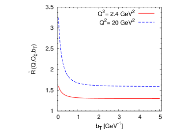
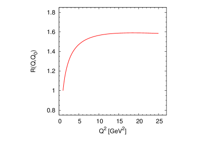
The TMD evolution in Eqs. (23)-(25) implies, apart from the explicit Gaussian dependence, a further non trivial dependence on the parton impact parameter bTsubscript𝑏𝑇b_{T} through the evolution kernel R~(Q,Q0,bT)~𝑅𝑄subscript𝑄0subscript𝑏𝑇\widetilde{R}(Q,Q_{0},b_{T}) and the upper integration limit μbsubscript𝜇𝑏\mu_{b}, Eq. (4), which appears in Eq. (7); consequently, it needs to be evaluated numerically. However, the evolution equations can be solved analytically by making a simple approximation on this bTsubscript𝑏𝑇b_{T} dependence. A close examination of Eq. (4) shows that μbsubscript𝜇𝑏\mu_{b} is a decreasing function of bTsubscript𝑏𝑇b_{T} that very rapidly freezes to the constant value C1/bmax=μb(bT)subscript𝐶1subscript𝑏maxsubscript𝜇𝑏subscript𝑏𝑇C_{1}/b_{\rm max}=\mu_{b}(b_{T}\to\infty): more precisely, the approximation μb=const.subscript𝜇𝑏𝑐𝑜𝑛𝑠𝑡\mu_{b}=const. holds for any bT >1 >subscript𝑏𝑇1b_{T}\mathrel{\hbox to0.0pt{\lower 4.0pt\hbox{\hskip 1.0pt$\sim$}\hss}\raise 1.0pt\hbox{$>$}}1 GeV-1. As very small values of bTsubscript𝑏𝑇b_{T} correspond to very large values of ksubscript𝑘perpendicular-tok_{\perp}, this approximation is safe in our framework, where the typical ksubscript𝑘perpendicular-tok_{\perp} are less than 111 GeV. Neglecting the bTsubscript𝑏𝑇b_{T}-dependence of μbsubscript𝜇𝑏\mu_{b}, the factor R~(Q,Q0,bT)~𝑅𝑄subscript𝑄0subscript𝑏𝑇\widetilde{R}(Q,Q_{0},b_{T}) does not depend on bTsubscript𝑏𝑇b_{T} anymore, see Eq. (7), and can even be integrated analytically by using an explicit representation of αs(Q)subscript𝛼𝑠𝑄\alpha_{s}(Q). In the sequel we will refer to it as R(Q,Q0)𝑅𝑄subscript𝑄0R(Q,Q_{0}), with R(Q,Q0)R~(Q,Q0,bT)𝑅𝑄subscript𝑄0~𝑅𝑄subscript𝑄0subscript𝑏𝑇R(Q,Q_{0})\equiv\widetilde{R}(Q,Q_{0},b_{T}\to\infty). Fig. 1 shows the evolution factor R~(Q,Q0,bT)~𝑅𝑄subscript𝑄0subscript𝑏𝑇\widetilde{R}(Q,Q_{0},b_{T}) plotted as a function of bTsubscript𝑏𝑇b_{T} at two fixed values of Q2superscript𝑄2Q^{2} (left panel), and R(Q,Q0)𝑅𝑄subscript𝑄0R(Q,Q_{0}) as a function of Q2superscript𝑄2Q^{2} (right panel). It is clear that R(Q,Q0)𝑅𝑄subscript𝑄0R(Q,Q_{0}) settles to a constant value for bT >1 >subscript𝑏𝑇1b_{T}\mathrel{\hbox to0.0pt{\lower 4.0pt\hbox{\hskip 1.0pt$\sim$}\hss}\raise 1.0pt\hbox{$>$}}1 GeV-1. In both cases, Q02=1superscriptsubscript𝑄021Q_{0}^{2}=1 GeV2.

Thus, in this approximation, the TMD evolution equation (6) only depends on bTsubscript𝑏𝑇b_{T} through the non-perturbative function gK(bT)subscript𝑔𝐾subscript𝑏𝑇g_{K}(b_{T}), which has been chosen to be a quadratic function of bTsubscript𝑏𝑇b_{T}, Eq. (13), and through the bTsubscript𝑏𝑇b_{T} dependence of the initial input function F~(x,𝒃T;Q0)~𝐹𝑥subscript𝒃𝑇subscript𝑄0\widetilde{F}(x,\mbox{\boldmath$b$}_{T};Q_{0}) which has been chosen to be Gaussian. It results in a bTsubscript𝑏𝑇b_{T}-Gaussian form, with a width which depends logarithmically on Q/Q0𝑄subscript𝑄0Q/Q_{0}, for the TMD evolution equation. For the unpolarized TMD PDFs one has

f~q/p(x,𝒃T;Q)=fq/p(x,Q0)R(Q,Q0)exp{bT24(k2+2g2lnQQ0)}.subscript~𝑓𝑞𝑝𝑥subscript𝒃𝑇𝑄subscript𝑓𝑞𝑝𝑥subscript𝑄0𝑅𝑄subscript𝑄0superscriptsubscript𝑏𝑇24delimited-⟨⟩superscriptsubscript𝑘perpendicular-to22subscript𝑔2𝑄subscript𝑄0\widetilde{f}_{q/p}(x,\mbox{\boldmath$b$}_{T};Q)=f_{q/p}(x,Q_{0})\;R(Q,Q_{0})\;\exp\left\{-\frac{b_{T}^{2}}{4}\left(\langle k_{\perp}^{2}\rangle+2\,g_{2}\ln\frac{Q}{Q_{0}}\right)\right\}\>. (26)
Refer to caption
Refer to caption
Figure 1: In the left panel, the evolution factor R(Q,Q0,bT)𝑅𝑄subscript𝑄0subscript𝑏𝑇R(Q,Q_{0},b_{T}) is plotted as a function of bTsubscript𝑏𝑇b_{T} at two fixed values of Q2superscript𝑄2Q^{2}. In the right panel we show R(Q,Q0)R(Q,Q0,bT)𝑅𝑄subscript𝑄0𝑅𝑄subscript𝑄0subscript𝑏𝑇R(Q,Q_{0})\equiv R(Q,Q_{0},b_{T}\to\infty) as a function of Q2superscript𝑄2Q^{2}. In both cases, Q02=1superscriptsubscript𝑄021Q_{0}^{2}=1 GeV2.

Its Fourier-transform, Eqs. (8), delivers a Gaussian distribution in the transverse momentum space as well:

f^q/p(x,k;Q)=fq/p(x,Q0)R(Q,Q0)ek2/w2πw2,subscript^𝑓𝑞𝑝𝑥subscript𝑘perpendicular-to𝑄subscript𝑓𝑞𝑝𝑥subscript𝑄0𝑅𝑄subscript𝑄0superscript𝑒superscriptsubscript𝑘perpendicular-to2superscript𝑤2𝜋superscript𝑤2\widehat{f}_{q/p}(x,k_{\perp};Q)=f_{q/p}(x,Q_{0})\;R(Q,Q_{0})\;\frac{e^{-k_{\perp}^{2}/w^{2}}}{\pi\,w^{2}}\>,\quad\quad (27)

where fq/p(x,Q0)subscript𝑓𝑞𝑝𝑥subscript𝑄0f_{q/p}(x,Q_{0}) is the usual integrated PDF evaluated at the initial scale Q0subscript𝑄0Q_{0} and, most importantly, w2w2(Q,Q0)superscript𝑤2superscript𝑤2𝑄subscript𝑄0w^{2}\equiv w^{2}(Q,Q_{0}) is the “evolving” Gaussian width, defined as:

w2(Q,Q0)=k2+2g2lnQQ0w^{2}(Q,Q_{0})=\langle k_{\perp}^{2}\rangle+2\,g_{2}\ln\frac{Q}{Q_{0}}\>\cdot (28)

It is worth noticing that the Q2superscript𝑄2Q^{2} evolution of the TMD PDFs is now determined by the overall factor R(Q,Q0)𝑅𝑄subscript𝑄0R(Q,Q_{0}) and, most crucially, by the Q2superscript𝑄2Q^{2} dependent Gaussian width w(Q,Q0)𝑤𝑄subscript𝑄0w(Q,Q_{0}).

The TMD FFs evolve in a similar way, Eq. (24),

D~h/q(z,bT;Q)=1z2Dh/q(z,Q0)R(Q,Q0)exp{bT24z2(p2+2z2g2lnQQ0)},subscript~𝐷𝑞𝑧subscript𝑏𝑇𝑄1superscript𝑧2subscript𝐷𝑞𝑧subscript𝑄0𝑅𝑄subscript𝑄0superscriptsubscript𝑏𝑇24superscript𝑧2delimited-⟨⟩superscriptsubscript𝑝perpendicular-to22superscript𝑧2subscript𝑔2𝑄subscript𝑄0\widetilde{D}_{h/q}(z,b_{T};Q)=\frac{1}{z^{2}}D_{h/q}(z,Q_{0})\;R(Q,Q_{0})\;\exp\left\{-\frac{b_{T}^{2}}{4\,z^{2}}\left(\langle p_{\perp}^{2}\rangle\,+2\,z^{2}\,g_{2}\ln\frac{Q}{Q_{0}}\right)\right\}\>, (29)

leading to the TMD FF in momentum space,

D^h/q(z,p;Q)=Dh/q(z,Q0)R(Q,Q0)ep2/wF2πwF2,subscript^𝐷𝑞𝑧subscript𝑝perpendicular-to𝑄subscript𝐷𝑞𝑧subscript𝑄0𝑅𝑄subscript𝑄0superscript𝑒superscriptsubscript𝑝perpendicular-to2subscriptsuperscript𝑤2𝐹𝜋subscriptsuperscript𝑤2𝐹\widehat{D}_{h/q}(z,p_{\perp};Q)=D_{h/q}(z,Q_{0})\;R(Q,Q_{0})\;\frac{e^{-p_{\perp}^{2}/w^{2}_{\!F}}}{\pi w^{2}_{\!F}}\>, (30)

with an evolving and z𝑧z-dependent Gaussian width wFwF(Q,Q0)subscript𝑤𝐹subscript𝑤𝐹𝑄subscript𝑄0w_{\!F}\equiv w_{\!F}(Q,Q_{0}) given by

wF2wF2(Q,Q0)=p2+2z2g2lnQQ0w_{\!F}^{2}\equiv w_{\!F}^{2}(Q,Q_{0})=\langle p_{\perp}^{2}\rangle+2z^{2}g_{2}\ln\frac{Q}{Q_{0}}\>\cdot (31)

For the Sivers distribution function, by Fourier-transforming Eq. (25) (with R~R~𝑅𝑅\widetilde{R}\to R) as prescribed by Eq. (10), we obtain [see also Eqs. (11), (12), (20) and (21)]:

ΔNf^q/p(x,k;Q)=kM12ek2S2k2ΔNfq/p(x,Q0)R(Q,Q0)ek2/wS2πwS4,superscriptΔ𝑁subscript^𝑓𝑞superscript𝑝𝑥subscript𝑘perpendicular-to𝑄subscript𝑘perpendicular-tosubscript𝑀12𝑒superscriptsubscriptdelimited-⟨⟩superscriptsubscript𝑘perpendicular-to2𝑆2delimited-⟨⟩superscriptsubscript𝑘perpendicular-to2superscriptΔ𝑁subscript𝑓𝑞superscript𝑝𝑥subscript𝑄0𝑅𝑄subscript𝑄0superscript𝑒superscriptsubscript𝑘perpendicular-to2superscriptsubscript𝑤𝑆2𝜋superscriptsubscript𝑤𝑆4\Delta^{N}\widehat{f}_{q/p^{\uparrow}}(x,k_{\perp};Q)=\frac{k_{\perp}}{M_{1}}\,\sqrt{2e}\,\frac{\langle k_{\perp}^{2}\rangle_{S}^{2}}{\langle k_{\perp}^{2}\rangle}\,\Delta^{N}f_{q/p^{\uparrow}}(x,Q_{0})\,R(Q,Q_{0})\,\frac{e^{-k_{\perp}^{2}/w_{S}^{2}}}{\pi w_{S}^{4}}\>, (32)

with

wS2(Q,Q0)=k2S+2g2lnQQ0w^{2}_{S}(Q,Q_{0})=\langle k_{\perp}^{2}\rangle_{S}+2g_{2}\ln\frac{Q}{Q_{0}}\>\cdot (33)

It is interesting to notice that the evolution factor R(Q,Q0)𝑅𝑄subscript𝑄0R(Q,Q_{0}), controlling the TMD evolution according to Eqs. (27), (30) and (32) is the same for all functions (TMD PDFs, TMD FFs and Sivers ) and is flavor independent: consequently it will appear, squared, in both numerator and denominator of the Sivers azimuthal asymmetry and, approximately, cancel out. Therefore, we can safely conclude that most of the TMD evolution of azimuthal asymmetries is controlled by the logarithmic Q𝑄Q dependence of the ksubscript𝑘perpendicular-tok_{\perp} Gaussian widths w2(Q,Q0)superscript𝑤2𝑄subscript𝑄0w^{2}(Q,Q_{0}), Eqs. (28), (31) and (33). We will come back to this in Section II.
Refer to caption
Refer to caption
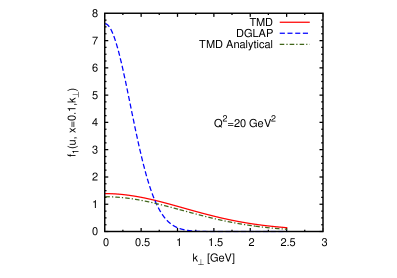
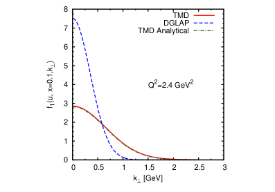
Figure 2: The left panel shows the unpolarized TMD PDF, f^u/psubscript^𝑓𝑢𝑝\widehat{f}_{u/p}, evolved from the initial scale, Q02=1superscriptsubscript𝑄021Q_{0}^{2}=1 GeV2, to Q2=2.4superscript𝑄22.4Q^{2}=2.4 GeV2, using TMD-evolution (red, solid line), DGLAP-evolution (blue, dashed line) and the analytical approximated TMD-evolution (green dot-dashed line). The right panel shows the same functions at the scale Q2=20superscript𝑄220Q^{2}=20 GeV2. Notice that, while there is hardly any difference between the DGLAP-evolved lines at Q2=2.4superscript𝑄22.4Q^{2}=2.4 and Q2=20superscript𝑄220Q^{2}=20 GeV2, the TMD evolution induces a fast decrease in size of the TMD PDF functions at large Q2superscript𝑄2Q^{2} and a simultaneous widening of its Gaussian width. Here the analytical approximated evolution gives results in good agreement with the exact calculation even at large Q2superscript𝑄2Q^{2}.
Refer to caption
Refer to caption
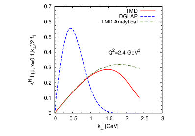
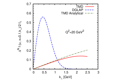
Figure 3: The left panel shows the ratio Sivers/PDF, ΔNf^u/p/2f^u/psuperscriptΔ𝑁subscript^𝑓𝑢superscript𝑝2subscript^𝑓𝑢𝑝\Delta^{N}\widehat{f}_{u/p^{\uparrow}}/2\widehat{f}_{u/p}, evolved from the initial scale, Q02=1superscriptsubscript𝑄021Q_{0}^{2}=1 GeV2, to Q2=2.4superscript𝑄22.4Q^{2}=2.4 GeV2, using TMD-evolution (red, solid line), DGLAP-evolution (blue, dashed line) and the analytical approximated TMD-evolution (green dot-dashed line). The right panel shows the same functions at the scale Q2=20superscript𝑄220Q^{2}=20 GeV2. Notice that, while there is almost no difference between the DGLAP-evolved lines at Q2=2.4superscript𝑄22.4Q^{2}=2.4 and Q2=20superscript𝑄220Q^{2}=20 GeV2, the TMD evolution induces a fast decrease in size of the ratio Sivers/PDF functions with growing Q2superscript𝑄2Q^{2} and a simultaneous widening of its Gaussian width. It is interesting to point out that the analytical approximation, for the Sivers function, visibly breaks down at large values of Q2superscript𝑄2Q^{2}.

To illustrate the features of this new TMD evolution, we compare it with the results obtained evolving only the collinear part, fq/p(x,Q)subscript𝑓𝑞𝑝𝑥𝑄f_{q/p}(x,Q), of the unpolarized TMD PDF according to the usual DGLAP equations and assuming the ksubscript𝑘perpendicular-tok_{\perp} dependent term of this function to be unaffected by evolution. In the left panel of Fig. 2 we show the ksubscript𝑘perpendicular-tok_{\perp} behavior of the unpolarized TMD PDF f^u/p(x,k,Q2)subscript^𝑓𝑢𝑝𝑥subscript𝑘perpendicular-tosuperscript𝑄2\widehat{f}_{u/p}(x,k_{\perp},Q^{2}), at the fixed value x=0.1𝑥0.1x=0.1, evaluated at the scale Q2=2.4superscript𝑄22.4Q^{2}=2.4 GeV2 (the average Q2superscript𝑄2Q^{2} value for the HERMES experiment). In the right panel we show the same function at a higher scale, Q2=20superscript𝑄220Q^{2}=20 GeV2 (which is the highest bin average Q2superscript𝑄2Q^{2} detected in the COMPASS experiment). In both cases the chosen initial scale is Q02=1superscriptsubscript𝑄021Q_{0}^{2}=1 GeV2. The red, solid line corresponds to the ksubscript𝑘perpendicular-tok_{\perp} distribution of the TMD PDF found by using the TMD-evolution of Eq. (23) while the blue, dashed line represents the result obtained by using DGLAP evolution equations. At the initial scale, Q02=1superscriptsubscript𝑄021Q_{0}^{2}=1 GeV2, solid and dashed curves coincide, by definition. However, while the DGLAP evolution is so slow that there is hardly any difference between the DGLAP-evolved lines at Q2=2.4superscript𝑄22.4Q^{2}=2.4 GeV2 and Q2=20superscript𝑄220Q^{2}=20 GeV2, the TMD evolution induces a fast decrease of the maximum values of the TMD PDF function with growing Q2superscript𝑄2Q^{2}, and a simultaneous broadening of its Gaussian width, as observed in Refs. Aybat:2011zv and Aybat:2011ge . It is interesting to notice that the approximated evolution of Eq. (27), corresponding to the green, dot-dashed line works really well, even for large Q2superscript𝑄2Q^{2} values.

A similar study is performed in Fig. 3 for the Sivers function. Here, by DGLAP evolution we mean that the Sivers function evolves like an unpolarized collinear PDF, only through the factor fq/p(x,Q)subscript𝑓𝑞𝑝𝑥𝑄f_{q/p}(x,Q) contained in its parameterization, Eq. (22). The parameters used for the plots are those given in Table 2, although any set of realistic parameters would lead to the same conclusions. The left panel shows the ratio between the Sivers function and the TMD PDF, ΔNf^u/p(x,k;Q)/(2f^u/p(x,k;Q))superscriptΔ𝑁subscript^𝑓𝑢superscript𝑝𝑥subscript𝑘perpendicular-to𝑄2subscript^𝑓𝑢𝑝𝑥subscript𝑘perpendicular-to𝑄\Delta^{N}\widehat{f}_{u/p^{\uparrow}}(x,k_{\perp};Q)/(2\widehat{f}_{u/p}(x,k_{\perp};Q)), evaluated at the scale Q2=2.4superscript𝑄22.4Q^{2}=2.4 GeV2. Again, the red, solid line is obtained using the TMD-evolution of Eqs. (23) and (25), while the blue, dashed line is given by the DGLAP-evolution. The green dot-dashed line represents the results obtained using the approximated analytical TMD-evolution of Eqs. (27) and (32). The right panel shows the same functions at the scale Q2=20superscript𝑄220Q^{2}=20 GeV2. Similarly to the case of TMD PDFs, while there is no difference between the DGLAP-evolved lines at Q2=2.4superscript𝑄22.4Q^{2}=2.4 and Q2=20superscript𝑄220Q^{2}=20 GeV2, the TMD evolution induces a fast decrease in the size of the TMD Sivers functions with growing Q2superscript𝑄2Q^{2} and a simultaneous widening of its Gaussian width. It is interesting to point out that the analytical TMD approximation, for the Sivers function visibly breaks down for large values of ksubscript𝑘perpendicular-tok_{\perp}.

II SIDIS data and TMD vs. non-TMD evolution

Having established the phenomenological formalism necessary to implement the TMD evolution, as given in Refs. Collins:2011book ; Aybat:2011zv ; Aybat:2011ge , we apply it to the Sivers function. This TMD distribution, ΔNf^q/p(x,k,Q)=(2k/Mp)f^1TsuperscriptΔ𝑁subscript^𝑓𝑞superscript𝑝𝑥subscript𝑘perpendicular-to𝑄2subscript𝑘perpendicular-tosubscript𝑀𝑝superscriptsubscript^𝑓1𝑇perpendicular-to\Delta^{N}\widehat{f}_{q/p^{\uparrow}}(x,k_{\perp},Q)=(-2k_{\perp}/M_{p})\widehat{f}_{1T}^{\perp}, can be extracted from HERMES and COMPASS phX𝑝𝑋\ell\,p\to h\,X SIDIS data on the azimuthal moment AUTsin(ϕhϕS)subscriptsuperscript𝐴subscriptitalic-ϕsubscriptitalic-ϕ𝑆𝑈𝑇A^{\sin(\phi_{h}-\phi_{S})}_{UT}, defined as

AUTsin(ϕhϕS)=2𝑑ϕS𝑑ϕh[dσdσ]sin(ϕhϕS)𝑑ϕS𝑑ϕh[dσ+dσ]A^{\sin(\phi_{h}-\phi_{S})}_{UT}=2\,\frac{\int d\phi_{S}\,d\phi_{h}\,[d\sigma^{\uparrow}-d\sigma^{\downarrow}]\,\sin(\phi_{h}-\phi_{S})}{\int d\phi_{S}\,d\phi_{h}\,[d\sigma^{\uparrow}+d\sigma^{\downarrow}]}\,\cdot (34)

This transverse single spin asymmetry (SSA) embeds the azimuthal modulation triggered by the correlation between the nucleon spin and the quark intrinsic transverse momentum. The “weighting” factor sin(ϕhϕS)subscriptitalic-ϕsubscriptitalic-ϕ𝑆\sin(\phi_{h}-\phi_{S}) in Eq. (34) is appropriately chosen to single out, among the various azimuthal dependent terms appearing in [dσdσ]delimited-[]𝑑superscript𝜎𝑑superscript𝜎[d\sigma^{\uparrow}-d\sigma^{\downarrow}], only the contribution of the Sivers mechanism Anselmino:2011ch ; Bacchetta:2006tn . By properly taking into account all intrinsic motions this transverse single spin asymmetry can be written as Anselmino:2005ea

AUTsin(ϕhϕS)=q𝑑ϕS𝑑ϕhd2𝒌ΔNf^q/p(x,k,Q)sin(φϕS)dσ^qqdQ2D^qh(z,p,Q)sin(ϕhϕS)q𝑑ϕS𝑑ϕhd2𝒌f^q/p(x,k,Q)dσ^qqdQ2D^qh(z,p,Q)A^{\sin(\phi_{h}-\phi_{S})}_{UT}=\frac{\displaystyle\sum_{q}\int{d\phi_{S}\,d\phi_{h}\,d^{2}\mbox{\boldmath$k$}_{\perp}}\;\Delta^{N}\widehat{f}_{q/p^{\uparrow}}(x,k_{\perp},Q)\;\sin(\varphi-\phi_{S})\;\frac{d\hat{\sigma}^{\ell q\to\ell q}}{dQ^{2}}\;\widehat{D}_{q}^{h}(z,p_{\perp},Q)\sin(\phi_{h}-\phi_{S})}{\displaystyle\sum_{q}\int{d\phi_{S}\,d\phi_{h}\,d^{2}\mbox{\boldmath$k$}_{\perp}}\;\widehat{f}_{q/p}(x,k_{\perp},Q)\;\frac{d\hat{\sigma}^{\ell q\to\ell q}}{dQ^{2}}\;\widehat{D}_{q}^{h}(z,p_{\perp},Q)}\>\cdot (35)

With respect to the leptonic plane, ϕSsubscriptitalic-ϕ𝑆\phi_{S} and ϕhsubscriptitalic-ϕ\phi_{h} are the azimuthal angles identifying the transverse directions of the proton spin 𝑺𝑺S and of the outgoing hadron hh respectively, while φ𝜑\varphi defines the direction of the incoming (and outgoing) quark transverse momentum, 𝒌subscript𝒌perpendicular-to\mbox{\boldmath$k$}_{\perp} = k(cosφ,sinφ,0)subscript𝑘perpendicular-to𝜑𝜑0k_{\perp}(\cos\varphi,\sin\varphi,0); dσ^qq/dQ2𝑑superscript^𝜎𝑞𝑞𝑑superscript𝑄2{d\hat{\sigma}^{\ell q\to\ell q}}/{dQ^{2}} is the unpolarized cross section for the elementary scattering qq𝑞𝑞\ell q\to\ell q.

The aim of our paper is to analyze the available polarized SIDIS data from the HERMES and COMPASS collaborations in order to understand whether or not they show signs of the TMD evolution proposed in Ref. Aybat:2011ge and described in Section I.1. Our general strategy is that of adopting the TMD evolution in the extraction of the Sivers functions, with the same parameterization and input functions as in Refs. Anselmino:2008sga ; Anselmino:2011gs , and see if that can improve the quality of the fits. In doing so we will make use of the HERMES re-analysis of SIDIS experimental data on Sivers asymmetries for pion and kaon production and the newest SIDIS COMPASS data off a proton target, which cover a wider range of Q2superscript𝑄2Q^{2} values, thus giving a better opportunity to check the TMD evolution.

In particular we perform three different data fits:

  • a fit (TMD-fit) in which we adopt the TMD evolution equation discussed in the Section I.1 and I.2, Eqs. (23)-(25) and (8)-(10);

  • a second fit (TMD-analytical-fit) in which we apply the same TMD evolution, but using the analytical approximation discussed in Section I.3, Eqs. (27), (30) and (32);

  • a fit (DGLAP-fit) in which we follow our previous work, as done so far in Ref. Anselmino:2008sga ; Anselmino:2011gs , using the DGLAP evolution equation only in the collinear part of the TMDs.

As a result of the fit we will have explicit expressions of all the Sivers functions and their parameters. However, the goal of the paper is not that of obtaining a new extraction of the Sivers distributions, although in the sequel we will show, for comment and illustration purposes, the Sivers functions for u𝑢u and d𝑑d valence quarks, with the relative parameters. The procedure followed here aims at testing the effect of the TMD evolution, as compared with the simple DGLAP evolution so far adopted, in fitting the TMD SIDIS data. If it turns out, as it will, that this improves the quality of the fit, then a new extraction of the Sivers distributions, entirely guided by the TMD evolution, will be necessary. That will require a different approach from the very beginning, with different input functions and parameterizations.

Here, we parameterize the Sivers function at the initial scale Q0=1subscript𝑄01Q_{0}=1 GeV, as in Ref. Anselmino:2008sga ; Anselmino:2011gs , in the following form:

ΔNf^q/p(x,k,Q0)=ΔNfq/p(x,Q0)h(k)=2𝒩q(x)h(k)f^q/p(x,k,Q0),superscriptΔ𝑁subscript^𝑓𝑞superscript𝑝𝑥subscript𝑘perpendicular-tosubscript𝑄0superscriptΔ𝑁subscript𝑓𝑞superscript𝑝𝑥subscript𝑄0subscript𝑘perpendicular-to2subscript𝒩𝑞𝑥subscript𝑘perpendicular-tosubscript^𝑓𝑞𝑝𝑥subscript𝑘perpendicular-tosubscript𝑄0\Delta^{N}\widehat{f}_{q/p^{\uparrow}}(x,k_{\perp},Q_{0})=\Delta^{N}\!f_{q/p^{\uparrow}}(x,Q_{0})\,h(k_{\perp})=2\,{\cal N}_{q}(x)\,h(k_{\perp})\,\widehat{f}_{q/p}(x,k_{\perp},Q_{0})\;, (36)

with

𝒩q(x)=Nqxαq(1x)βq(αq+βq)(αq+βq)αqαqβqβq,subscript𝒩𝑞𝑥subscript𝑁𝑞superscript𝑥subscript𝛼𝑞superscript1𝑥subscript𝛽𝑞superscriptsubscript𝛼𝑞subscript𝛽𝑞subscript𝛼𝑞subscript𝛽𝑞superscriptsubscript𝛼𝑞subscript𝛼𝑞superscriptsubscript𝛽𝑞subscript𝛽𝑞\displaystyle{\cal N}_{q}(x)=N_{q}\,x^{\alpha_{q}}(1-x)^{\beta_{q}}\,\frac{(\alpha_{q}+\beta_{q})^{(\alpha_{q}+\beta_{q})}}{\alpha_{q}^{\alpha_{q}}\beta_{q}^{\beta_{q}}}\;, (37)
h(k)=2ekM1ek2/M12,subscript𝑘perpendicular-to2𝑒subscript𝑘perpendicular-tosubscript𝑀1superscript𝑒superscriptsubscript𝑘perpendicular-to2superscriptsubscript𝑀12\displaystyle h(k_{\perp})=\sqrt{2e}\,\frac{k_{\perp}}{M_{1}}\,e^{-{k_{\perp}^{2}}/{M_{1}^{2}}}\;, (38)

where f^q/p(x,k,Q0)subscript^𝑓𝑞𝑝𝑥subscript𝑘perpendicular-tosubscript𝑄0\widehat{f}_{q/p}(x,k_{\perp},Q_{0}) is defined in Eq. 15 and Nqsubscript𝑁𝑞N_{q}, αqsubscript𝛼𝑞\alpha_{q}, βqsubscript𝛽𝑞\beta_{q} and M1subscript𝑀1M_{1} (GeV) are (scale independent) free parameters to be determined by fitting the experimental data. Since h(k)1subscript𝑘perpendicular-to1h(k_{\perp})\leq 1 for any ksubscript𝑘perpendicular-tok_{\perp} and |𝒩q(x)|1subscript𝒩𝑞𝑥1|{\cal N}_{q}(x)|\leq 1 for any x𝑥x (notice that we allow the constant parameter Nqsubscript𝑁𝑞N_{q} to vary only inside the range [1,1]11[-1,1]), the positivity bound for the Sivers function,

|ΔNf^q/p(x,k)|2f^q/p(x,k)1,superscriptΔ𝑁subscript^𝑓𝑞superscript𝑝𝑥subscript𝑘perpendicular-to2subscript^𝑓𝑞𝑝𝑥subscript𝑘perpendicular-to1\frac{|\Delta^{N}\widehat{f}_{q/p^{\uparrow}}(x,k_{\perp})|}{2\widehat{f}_{q/p}(x,k_{\perp})}\leq 1\>, (39)

is automatically fulfilled. Similarly to PDFs, the FFs at the initial scale are parameterized with a Gaussian shape, Eq. (17).

As in Refs. Anselmino:2005nn and Anselmino:2008sga , the average values of ksubscript𝑘perpendicular-tok_{\perp} and psubscript𝑝perpendicular-top_{\perp} are fixed as

k2=0.25GeV2p2=0.20GeV2.formulae-sequencedelimited-⟨⟩superscriptsubscript𝑘perpendicular-to20.25superscriptGeV2delimited-⟨⟩superscriptsubscript𝑝perpendicular-to20.20superscriptGeV2\langle k_{\perp}^{2}\rangle=0.25\;{\rm GeV}^{2}\quad\quad\quad\langle p_{\perp}^{2}\rangle=0.20\;{\rm GeV}^{2}\>. (40)

We take the unpolarized distributions fq/p(x,Q02)subscript𝑓𝑞𝑝𝑥subscriptsuperscript𝑄20f_{q/p}(x,Q^{2}_{0}) from Ref. Gluck:1998xa and the unpolarized fragmentation functions Dh/q(z,Q02)subscript𝐷𝑞𝑧subscriptsuperscript𝑄20D_{h/q}(z,Q^{2}_{0}) from Ref. deFlorian:2007aj , with Q02=1.0subscriptsuperscript𝑄201.0Q^{2}_{0}=1.0 GeV. As in Ref. Anselmino:2008sga , we adopt 11 free parameters:

NuvNdvNssubscript𝑁subscript𝑢𝑣subscript𝑁subscript𝑑𝑣subscript𝑁𝑠\displaystyle N_{u_{v}}\quad\quad\quad N_{d_{v}}\quad\quad\quad N_{s}
Nu¯Nd¯Ns¯subscript𝑁¯𝑢subscript𝑁¯𝑑subscript𝑁¯𝑠\displaystyle N_{\bar{u}}\quad\quad\quad\;\,N_{\bar{d}}\quad\quad\quad\;N_{\bar{s}}
αuvαdvαseasubscript𝛼subscript𝑢𝑣subscript𝛼subscript𝑑𝑣subscript𝛼𝑠𝑒𝑎\displaystyle\alpha_{u_{v}}\quad\quad\quad\,\alpha_{d_{v}}\quad\quad\quad\,\alpha_{sea} (41)
βM1(GeV),𝛽subscript𝑀1GeV\displaystyle\beta\quad\quad\quad\,\,\,\;\;M_{1}\;({\rm GeV})\>,

where the subscript v𝑣v denotes valence contributions. In this choice we differ from Ref. Anselmino:2008sga , where valence and sea contributions were not separated.

We perform best fits of 111111 experimental data sets: HERMES :2009ti data for SIDIS production of pions (π+superscript𝜋\pi^{+}, πsuperscript𝜋\pi^{-}, π0superscript𝜋0\pi^{0}) and kaons (K+superscript𝐾K^{+} and Ksuperscript𝐾K^{-}), COMPASS data for SIDIS pion (π+superscript𝜋\pi^{+}, πsuperscript𝜋\pi^{-}) and kaon (K+superscript𝐾K^{+} and Ksuperscript𝐾K^{-}) production from a LiD𝐿𝑖𝐷LiD (deuteron) target :2008dn , and the preliminary COMPASS data for charged hadron production from an NH3𝑁subscript𝐻3NH_{3} (proton) target Bradamante:2011xu . The results of these 3 fits are presented in Table 1 in terms of their χ2superscript𝜒2\chi^{2}s.

Table 1: χ2superscript𝜒2\chi^{2} contributions corresponding to the TMD-fit, the TMD-analytical-fit and the DGLAP-fit, for each experimental data set of HERMES and COMPASS experiments.
TMD Evolution (exact) TMD Evolution (analytical) DGLAP Evolution
χtot2=255.8subscriptsuperscript𝜒2𝑡𝑜𝑡255.8\chi^{2}_{tot}\;=255.8 χtot2=275.7subscriptsuperscript𝜒2𝑡𝑜𝑡275.7\chi^{2}_{tot}\;=275.7 χtot2=315.6subscriptsuperscript𝜒2𝑡𝑜𝑡315.6\chi^{2}_{tot}\;=315.6
χd.o.f2= 1.02subscriptsuperscript𝜒2formulae-sequence𝑑𝑜𝑓1.02\chi^{2}_{d.o.f}=\;1.02 χd.o.f2= 1.10subscriptsuperscript𝜒2formulae-sequence𝑑𝑜𝑓1.10\chi^{2}_{d.o.f}=\;1.10 χd.o.f2= 1.26subscriptsuperscript𝜒2formulae-sequence𝑑𝑜𝑓1.26\chi^{2}_{d.o.f}=\;1.26
Experiment Hadron N. points
7 χx2=10.7subscriptsuperscript𝜒2𝑥10.7\chi^{2}_{x}\;=10.7 χx2=12.9subscriptsuperscript𝜒2𝑥12.9\chi^{2}_{x}\;=12.9 χx2=27.5subscriptsuperscript𝜒2𝑥27.5\chi^{2}_{x}\;=27.5
π+superscript𝜋\pi^{+} 7 χz2= 4.3subscriptsuperscript𝜒2𝑧4.3\chi^{2}_{z}\;=\;4.3 χz2= 4.3subscriptsuperscript𝜒2𝑧4.3\chi^{2}_{z}\;=\;4.3 χz2=8.6subscriptsuperscript𝜒2𝑧8.6\chi^{2}_{z}\;=8.6
7 χPT2=9.1subscriptsuperscript𝜒2subscript𝑃𝑇9.1\chi^{2}_{P_{T}}\!=9.1 χPT2=10.5subscriptsuperscript𝜒2subscript𝑃𝑇10.5\chi^{2}_{P_{T}}\!=10.5 χPT2=22.5subscriptsuperscript𝜒2subscript𝑃𝑇22.5\chi^{2}_{P_{T}}\!=22.5
7 χx2=17.0subscriptsuperscript𝜒2𝑥17.0\chi^{2}_{x}=17.0 χx2=16.5subscriptsuperscript𝜒2𝑥16.5\chi^{2}_{x}=16.5 χx2=14.8subscriptsuperscript𝜒2𝑥14.8\chi^{2}_{x}=14.8
πsuperscript𝜋\pi^{-} 7 χz2= 2.4subscriptsuperscript𝜒2𝑧2.4\chi^{2}_{z}=\;2.4 χz2= 2.4subscriptsuperscript𝜒2𝑧2.4\chi^{2}_{z}=\;2.4 χz2= 3.3subscriptsuperscript𝜒2𝑧3.3\chi^{2}_{z}=\;3.3
7 χPT2=6.4subscriptsuperscript𝜒2subscript𝑃𝑇6.4\chi^{2}_{P_{T}}\!=6.4 χPT2=6.3subscriptsuperscript𝜒2subscript𝑃𝑇6.3\chi^{2}_{P_{T}}\!=6.3 χPT2=6.2subscriptsuperscript𝜒2subscript𝑃𝑇6.2\chi^{2}_{P_{T}}\!=6.2
7 χx2= 5.9subscriptsuperscript𝜒2𝑥5.9\chi^{2}_{x}=\;5.9 χx2= 5.8subscriptsuperscript𝜒2𝑥5.8\chi^{2}_{x}=\;5.8 χx2= 5.6subscriptsuperscript𝜒2𝑥5.6\chi^{2}_{x}=\;5.6
HERMES π0superscript𝜋0\pi^{0} 7 χz2= 8.0subscriptsuperscript𝜒2𝑧8.0\chi^{2}_{z}=\;8.0 χz2= 8.1subscriptsuperscript𝜒2𝑧8.1\chi^{2}_{z}=\;8.1 χz2= 6.9subscriptsuperscript𝜒2𝑧6.9\chi^{2}_{z}=\;6.9
7 χPT2=6.8subscriptsuperscript𝜒2subscript𝑃𝑇6.8\chi^{2}_{P_{T}}\!=6.8 χPT2=7.0subscriptsuperscript𝜒2subscript𝑃𝑇7.0\chi^{2}_{P_{T}}\!=7.0 χPT2=6.6subscriptsuperscript𝜒2subscript𝑃𝑇6.6\chi^{2}_{P_{T}}\!=6.6
7 χx2= 4.7subscriptsuperscript𝜒2𝑥4.7\chi^{2}_{x}=\;4.7 χx2= 4.8subscriptsuperscript𝜒2𝑥4.8\chi^{2}_{x}=\;4.8 χx2= 4.4subscriptsuperscript𝜒2𝑥4.4\chi^{2}_{x}=\;4.4
K+superscript𝐾K^{+} 7 χz2= 9.3subscriptsuperscript𝜒2𝑧9.3\chi^{2}_{z}=\;9.3 χz2= 9.8subscriptsuperscript𝜒2𝑧9.8\chi^{2}_{z}=\;9.8 χz2= 4.3subscriptsuperscript𝜒2𝑧4.3\chi^{2}_{z}=\;4.3
7 χPT2=4.6subscriptsuperscript𝜒2subscript𝑃𝑇4.6\chi^{2}_{P_{T}}\!=4.6 χPT2=5.3subscriptsuperscript𝜒2subscript𝑃𝑇5.3\chi^{2}_{P_{T}}\!=5.3 χPT2=2.8subscriptsuperscript𝜒2subscript𝑃𝑇2.8\chi^{2}_{P_{T}}\!=2.8
7 χx2= 2.4subscriptsuperscript𝜒2𝑥2.4\chi^{2}_{x}=\;2.4 χx2= 2.4subscriptsuperscript𝜒2𝑥2.4\chi^{2}_{x}=\;2.4 χx2= 2.9subscriptsuperscript𝜒2𝑥2.9\chi^{2}_{x}=\;2.9
Ksuperscript𝐾K^{-} 7 χz2= 7.2subscriptsuperscript𝜒2𝑧7.2\chi^{2}_{z}=\;7.2 χz2= 7.0subscriptsuperscript𝜒2𝑧7.0\chi^{2}_{z}=\;7.0 χz2= 5.5subscriptsuperscript𝜒2𝑧5.5\chi^{2}_{z}=\;5.5
7 χPT2=3.4subscriptsuperscript𝜒2subscript𝑃𝑇3.4\chi^{2}_{P_{T}}\!=3.4 χPT2=3.3subscriptsuperscript𝜒2subscript𝑃𝑇3.3\chi^{2}_{P_{T}}\!=3.3 χPT2=3.7subscriptsuperscript𝜒2subscript𝑃𝑇3.7\chi^{2}_{P_{T}}\!=3.7
9 χx2= 6.7subscriptsuperscript𝜒2𝑥6.7\chi^{2}_{x}=\;6.7 χx2=11.2subscriptsuperscript𝜒2𝑥11.2\chi^{2}_{x}=11.2 χx2=29.2subscriptsuperscript𝜒2𝑥29.2\chi^{2}_{x}=29.2
h+superscripth^{+} 8 χz2=17.8subscriptsuperscript𝜒2𝑧17.8\chi^{2}_{z}=17.8 χz2=18.5subscriptsuperscript𝜒2𝑧18.5\chi^{2}_{z}=18.5 χz2=16.6subscriptsuperscript𝜒2𝑧16.6\chi^{2}_{z}=16.6
COMPASS-p 9 χPT2=12.4subscriptsuperscript𝜒2subscript𝑃𝑇12.4\chi^{2}_{P_{T}}\!=12.4 χPT2=24.2subscriptsuperscript𝜒2subscript𝑃𝑇24.2\chi^{2}_{P_{T}}\!=24.2 χPT2=11.8subscriptsuperscript𝜒2subscript𝑃𝑇11.8\chi^{2}_{P_{T}}\!=11.8
9 χx2= 7.6subscriptsuperscript𝜒2𝑥7.6\chi^{2}_{x}=\;7.6 χx2= 7.7subscriptsuperscript𝜒2𝑥7.7\chi^{2}_{x}=\;7.7 χx2=11.9subscriptsuperscript𝜒2𝑥11.9\chi^{2}_{x}=11.9
hsuperscripth^{-} 8 χz2= 9.7subscriptsuperscript𝜒2𝑧9.7\chi^{2}_{z}=\;9.7 χz2= 9.6subscriptsuperscript𝜒2𝑧9.6\chi^{2}_{z}=\;9.6 χz2=14.1subscriptsuperscript𝜒2𝑧14.1\chi^{2}_{z}=14.1
9 χPT2=8.1subscriptsuperscript𝜒2subscript𝑃𝑇8.1\chi^{2}_{P_{T}}\!=8.1 χPT2=8.1subscriptsuperscript𝜒2subscript𝑃𝑇8.1\chi^{2}_{P_{T}}\!=8.1 χPT2=9.9subscriptsuperscript𝜒2subscript𝑃𝑇9.9\chi^{2}_{P_{T}}\!=9.9
9 χx2= 7.3subscriptsuperscript𝜒2𝑥7.3\chi^{2}_{x}=\;7.3 χx2= 7.1subscriptsuperscript𝜒2𝑥7.1\chi^{2}_{x}=\;7.1 χx2= 5.3subscriptsuperscript𝜒2𝑥5.3\chi^{2}_{x}=\;5.3
π+superscript𝜋\pi^{+} 8 χz2= 5.4subscriptsuperscript𝜒2𝑧5.4\chi^{2}_{z}=\;5.4 χz2= 5.3subscriptsuperscript𝜒2𝑧5.3\chi^{2}_{z}=\;5.3 χz2= 7.9subscriptsuperscript𝜒2𝑧7.9\chi^{2}_{z}=\;7.9
9 χPT2=5.4subscriptsuperscript𝜒2subscript𝑃𝑇5.4\chi^{2}_{P_{T}}\!=5.4 χPT2=5.2subscriptsuperscript𝜒2subscript𝑃𝑇5.2\chi^{2}_{P_{T}}\!=5.2 χPT2=5.5subscriptsuperscript𝜒2subscript𝑃𝑇5.5\chi^{2}_{P_{T}}\!=5.5
9 χx2= 4.4subscriptsuperscript𝜒2𝑥4.4\chi^{2}_{x}=\;4.4 χx2= 4.4subscriptsuperscript𝜒2𝑥4.4\chi^{2}_{x}=\;4.4 χx2= 5.0subscriptsuperscript𝜒2𝑥5.0\chi^{2}_{x}=\;5.0
πsuperscript𝜋\pi^{-} 8 χz2=10.9subscriptsuperscript𝜒2𝑧10.9\chi^{2}_{z}=10.9 χz2=10.7subscriptsuperscript𝜒2𝑧10.7\chi^{2}_{z}=10.7 χz2=13.9subscriptsuperscript𝜒2𝑧13.9\chi^{2}_{z}=13.9
COMPASS-d 9 χPT2=4.5subscriptsuperscript𝜒2subscript𝑃𝑇4.5\chi^{2}_{P_{T}}\!=4.5 χPT2=4.8subscriptsuperscript𝜒2subscript𝑃𝑇4.8\chi^{2}_{P_{T}}\!=4.8 χPT2=4.4subscriptsuperscript𝜒2subscript𝑃𝑇4.4\chi^{2}_{P_{T}}\!=4.4
9 χx2= 6.5subscriptsuperscript𝜒2𝑥6.5\chi^{2}_{x}=\;6.5 χx2= 6.5subscriptsuperscript𝜒2𝑥6.5\chi^{2}_{x}=\;6.5 χx2= 5.8subscriptsuperscript𝜒2𝑥5.8\chi^{2}_{x}=\;5.8
K+superscript𝐾K^{+} 8 χz2= 7.7subscriptsuperscript𝜒2𝑧7.7\chi^{2}_{z}=\;7.7 χz2= 7.7subscriptsuperscript𝜒2𝑧7.7\chi^{2}_{z}=\;7.7 χz2= 7.2subscriptsuperscript𝜒2𝑧7.2\chi^{2}_{z}=\;7.2
9 χPT2=4.8subscriptsuperscript𝜒2subscript𝑃𝑇4.8\chi^{2}_{P_{T}}\!=4.8 χPT2=4.9subscriptsuperscript𝜒2subscript𝑃𝑇4.9\chi^{2}_{P_{T}}\!=4.9 χPT2=4.7subscriptsuperscript𝜒2subscript𝑃𝑇4.7\chi^{2}_{P_{T}}\!=4.7
9 χx2=12.1subscriptsuperscript𝜒2𝑥12.1\chi^{2}_{x}=12.1 χx2=12.4subscriptsuperscript𝜒2𝑥12.4\chi^{2}_{x}=12.4 χx2=13.1subscriptsuperscript𝜒2𝑥13.1\chi^{2}_{x}=13.1
Ksuperscript𝐾K^{-} 8 χz2= 8.9subscriptsuperscript𝜒2𝑧8.9\chi^{2}_{z}=\;8.9 χz2= 9.0subscriptsuperscript𝜒2𝑧9.0\chi^{2}_{z}=\;9.0 χz2=9.4subscriptsuperscript𝜒2𝑧9.4\chi^{2}_{z}=9.4
9 χPT2=13.5subscriptsuperscript𝜒2subscript𝑃𝑇13.5\chi^{2}_{P_{T}}\!=13.5 χPT2=12.0subscriptsuperscript𝜒2subscript𝑃𝑇12.0\chi^{2}_{P_{T}}\!=12.0 χPT2=14.4subscriptsuperscript𝜒2subscript𝑃𝑇14.4\chi^{2}_{P_{T}}\!=14.4

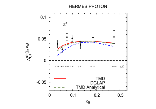
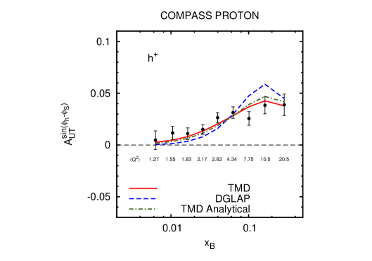
As it is clear from the first line of Table I, the best total χtot2subscriptsuperscript𝜒2𝑡𝑜𝑡\chi^{2}_{tot}, which amounts to 256256256, is obtained by using the TMD evolution, followed by a slightly higher χtot2subscriptsuperscript𝜒2𝑡𝑜𝑡\chi^{2}_{tot} of the analytical approximation, and a definitely larger χtot2316similar-to-or-equalssubscriptsuperscript𝜒2𝑡𝑜𝑡316\chi^{2}_{tot}\simeq 316 corresponding to the DGLAP fit. To examine the origin of this difference between TMD and DGLAP evolution, we show the individual contributions to χtot2subscriptsuperscript𝜒2𝑡𝑜𝑡\chi^{2}_{tot} of each experiment (HERMES, COMPASS on NH3𝑁subscript𝐻3NH_{3} and on LiD𝐿𝑖𝐷LiD targets), for all types of detected hadrons and for all variables observed (x𝑥x, z𝑧z and PTsubscript𝑃𝑇P_{T}). A global look at the numbers reported in Table I shows that the difference of about 60 χ2superscript𝜒2\chi^{2}-points between the TMD and the DGLAP fits is not equally distributed among all χ2superscript𝜒2\chi^{2}s per data point; rather, it is heavily concentrated in three particular cases, namely in the asymmetry for π+superscript𝜋\pi^{+} production at HERMES and for h+superscripth^{+} and hsuperscripth^{-} production at COMPASS off a proton target, especially when this asymmetry is observed as a function of the x𝑥x-variable.

It is important to stress that, as x𝑥x is directly proportional to Q2superscript𝑄2Q^{2} through the kinematical relation Q2=xyssuperscript𝑄2𝑥𝑦𝑠Q^{2}=x\,y\,s, the x𝑥x behavior of the asymmetries is intimately connected to their Q2superscript𝑄2Q^{2} evolution. While the HERMES experimental bins cover a very modest range of Q2superscript𝑄2Q^{2} values, from 1.31.31.3 GeV2 to 6.26.26.2 GeV2, COMPASS data raise to a maximum Q2superscript𝑄2Q^{2} of 20.520.520.5 GeV2, enabling to test more severely the TMD Q2superscript𝑄2Q^{2} evolution in SIDIS.

These aspects are illustrated in Fig. 4, where the SIDIS Sivers asymmetries AUTsin(ϕhϕS)subscriptsuperscript𝐴subscriptitalic-ϕsubscriptitalic-ϕ𝑆𝑈𝑇A^{\sin(\phi_{h}-\phi_{S})}_{UT} obtained in the three fits are shown in the same plot. It is evident that the DGLAP evolution seems to be unable to describe the correct x𝑥x trend, i.e. the right Q2superscript𝑄2Q^{2} behavior, while the TMD evolution (red solid line) follows much better the large Q2superscript𝑄2Q^{2} data points, corresponding to the last x𝑥x-bins measured by COMPASS. The approximate analytical TMD evolution (green dash-dotted line) works very well for low to moderate values of Q2superscript𝑄2Q^{2} while it starts to deviate from the exact behavior at large Q2superscript𝑄2Q^{2} values.

Refer to caption
Refer to caption
Figure 4: The results obtained from our fit of the SIDIS AUTsin(ϕhϕS)superscriptsubscript𝐴𝑈𝑇subscriptitalic-ϕsubscriptitalic-ϕ𝑆A_{UT}^{\sin{(\phi_{h}-\phi_{S})}} Sivers asymmetries applying TMD evolution (red, solid lines) are compared with the analogous results found by using DGLAP evolution equations (blue, dashed lines). The green, dash-dotted lines correspond to the results obtained by using the approximated analytical TMD evolution (see text for further details). The experimental data are from HERMES :2009ti (left panel) and COMPASS Bradamante:2011xu (right panel) Collaborations.
Refer to caption
Refer to caption
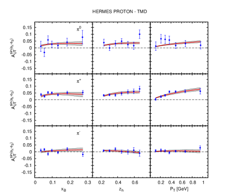
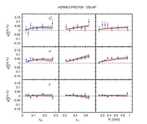
Figure 5: The results obtained from the TMD-evolution fit (left panel) and from the DGLAP-evolution fit (right panel) of the SIDIS AUTsin(ϕhϕS)superscriptsubscript𝐴𝑈𝑇subscriptitalic-ϕsubscriptitalic-ϕ𝑆A_{UT}^{\sin{(\phi_{h}-\phi_{S})}} Sivers asymmetries (red, solid lines) are compared with the HERMES experimental data :2009ti for charged and neutral pion production. The shaded area corresponds to the statistical uncertainty of the parameters, see Appendix A of Ref. Anselmino:2008sga for further details.
Refer to caption
Refer to caption
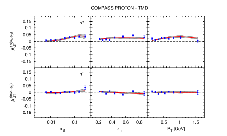
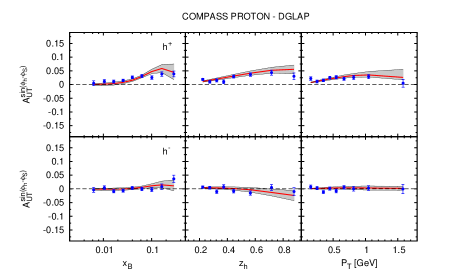
Figure 6: The results obtained from the TMD-evolution fit (left panel) and from the DGLAP-evolution fit (right panel) of the SIDIS AUTsin(ϕhϕS)superscriptsubscript𝐴𝑈𝑇subscriptitalic-ϕsubscriptitalic-ϕ𝑆A_{UT}^{\sin{(\phi_{h}-\phi_{S})}} Sivers asymmetries (red, solid lines) are compared with the COMPASS-p experimental data Bradamante:2011xu for charged hadron production. The shaded area corresponds to the statistical uncertainty of the parameters, see Appendix A of Ref. Anselmino:2008sga for further details.

In Figs. 5 we show, as an illustration of their qualities, our best fits (solid red lines) of the HERMES experimental data :2009ti on the Sivers asymmetries for pion production. Those on the left panels are obtained adopting the new TMD evolution, while those on the right use the simplified DGLAP evolution. Similar results are shown, for the recent COMPASS data off a proton target Bradamante:2011xu for charged hadron production, in Fig. 6.

The shaded area represents the statistical uncertainty of the fit parameters corresponding to a Δχ2=20Δsuperscript𝜒220\Delta\chi^{2}=20 (i.e. to 95.45%percent95.4595.45\% confidence level for 11 degrees of freedom, see Appendix A of Ref. Anselmino:2008sga for further details). Notice that, in general, the error bands corresponding to the TMD-evolution fit are thinner than those corresponding to the DGLAP fit: this is caused by the fact that the TMD evolution implies a ratio Sivers/PDF which becomes smaller with growing Q2superscript𝑄2Q^{2}, as shown in Fig. 3, constraining the free parameters much more tightly than in the DGLAP-evolution fit, where the Sivers/PDF ratio remains roughly constant as Q2superscript𝑄2Q^{2} raises from low to large values.

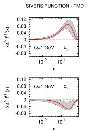
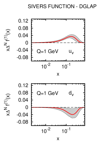
In Fig. 7 we compare, for illustration purposes, the Sivers function – actually, its first moment, defined in Ref. Anselmino:2008sga – at the initial scale Q0subscript𝑄0Q_{0} for u𝑢u and d𝑑d valence quarks, as obtained in our best fits with the TMD (left panel) and the DGLAP (right panel) evolution, Table 2. Notice that for this analysis we have chosen to separate valence from sea quark contributions, while in Ref. Anselmino:2008sga the u𝑢u and d𝑑d flavors included all contributions.

Refer to caption
Refer to caption
Figure 7: The first moment of the valence u𝑢u and d𝑑d Sivers functions, evaluated at Q=Q0𝑄subscript𝑄0Q=Q_{0}, obtained from our best fits of the AUTsin(ϕhϕS)superscriptsubscript𝐴𝑈𝑇subscriptitalic-ϕsubscriptitalic-ϕ𝑆A_{UT}^{\sin{(\phi_{h}-\phi_{S})}} azimuthal moments as measured by HERMES :2009ti and COMPASS Bradamante:2011xu ; :2008dn Collaborations. The extraction of the Sivers functions on the left side takes into account the TMD-evolution (left column of Table 2), while for those on the right side it does not (right column of Table 2). The shaded area corresponds to the statistical uncertainty of the parameters, see Appendix A of Ref. Anselmino:2008sga for further details.
Table 2: Best values of the free parameters, Eq. (41), for the Sivers functions of u𝑢u and d𝑑d valence quarks, as obtained from our TMD-fit, TMD-analytical-fit and DGLAP-fit, at Q0=1subscript𝑄01Q_{0}=1 GeV. The errors reported in this table correspond to the maximum and minimum values of each parameter in a restricted parameter space constrained by the condition Δχ2=20Δsuperscript𝜒220\Delta\chi^{2}=20, corresponding to 95.45%percent95.4595.45\% confidence level. They correspond to the shaded area in Fig. 7.
TMD Evolution (exact) TMD Evolution (analytical) DGLAP Evolution
Nuv=0.770.19+0.23subscript𝑁subscript𝑢𝑣subscriptsuperscript0.770.230.19N_{u_{v}}=0.77^{+0.23}_{-0.19} Nuv=0.750.21+0.25subscript𝑁subscript𝑢𝑣subscriptsuperscript0.750.250.21N_{u_{v}}=0.75^{+0.25}_{-0.21} Nuv=0.450.17+0.25subscript𝑁subscript𝑢𝑣subscriptsuperscript0.450.250.17N_{u_{v}}=0.45^{+0.25}_{-0.17}
Ndv=1.000.00+0.75subscript𝑁subscript𝑑𝑣subscriptsuperscript1.000.750.00N_{d_{v}}=-1.00^{+0.75}_{-0.00} Ndv=1.000.00+0.82subscript𝑁subscript𝑑𝑣subscriptsuperscript1.000.820.00N_{d_{v}}=-1.00^{+0.82}_{-0.00} Ndv=1.000.00+0.85subscript𝑁subscript𝑑𝑣subscriptsuperscript1.000.850.00N_{d_{v}}=-1.00^{+0.85}_{-0.00}
αuv=0.680.40+0.57subscript𝛼subscript𝑢𝑣subscriptsuperscript0.680.570.40\alpha_{u_{v}}=0.68^{+0.57}_{-0.40} αuv=0.820.48+0.51subscript𝛼subscript𝑢𝑣subscriptsuperscript0.820.510.48\alpha_{u_{v}}=0.82^{+0.51}_{-0.48} αuv=1.080.62+0.68subscript𝛼subscript𝑢𝑣subscriptsuperscript1.080.680.62\alpha_{u_{v}}=1.08^{+0.68}_{-0.62}
αdv=1.110.91+1.39subscript𝛼subscript𝑑𝑣subscriptsuperscript1.111.390.91\alpha_{d_{v}}=1.11^{+1.39}_{-0.91} αdv=1.361.00+1.24subscript𝛼subscript𝑑𝑣subscriptsuperscript1.361.241.00\alpha_{d_{v}}=1.36^{+1.24}_{-1.00} αdv=1.70.91+1.15subscript𝛼subscript𝑑𝑣subscriptsuperscript1.71.150.91\alpha_{d_{v}}=1.7^{+1.15}_{-0.91}
β=3.12.6+4.7𝛽subscriptsuperscript3.14.72.6\beta\;\;=3.1^{+4.7}_{-2.6} β=4.02.8+4.5𝛽subscriptsuperscript4.04.52.8\beta\;\;=4.0^{+4.5}_{-2.8} β=6.94.1+6.4𝛽subscriptsuperscript6.96.44.1\beta\;\;=6.9^{+6.4}_{-4.1}
M12=0.400.23+1.5superscriptsubscript𝑀12subscriptsuperscript0.401.50.23M_{1}^{2}=0.40^{+1.5}_{-0.23} GeV2 M12=0.340.19+1.36superscriptsubscript𝑀12subscriptsuperscript0.341.360.19M_{1}^{2}=0.34^{+1.36}_{-0.19} GeV2 M12=0.190.10+0.77superscriptsubscript𝑀12subscriptsuperscript0.190.770.10M_{1}^{2}=0.19^{+0.77}_{-0.10} GeV2

This result deserves some comments. The comparison shows that the extracted u𝑢u and d𝑑d valence contributions, at the initial scale Q0=1subscript𝑄01Q_{0}=1 GeV, are definitely larger for the TMD evolution fit. This reflects the TMD evolution property, according to which the Sivers functions are strongly suppressed with increasing Q2superscript𝑄2Q^{2}, which is not the case for the almost static collinear DGLAP evolution. Thus, in order to fit the same data at Q2superscript𝑄2Q^{2} bins ranging from 1.3 to 20.5 GeV2, the TMD evolving Sivers functions must start from higher values at Q0=1subscript𝑄01Q_{0}=1 GeV. The Sivers distributions previously extracted, with the DGLAP evolution, in Refs. Anselmino:2008sga ; Anselmino:2011gs were given at Q2=2.4superscript𝑄22.4Q^{2}=2.4 GeV2; one should notice that if we TMD evolve the Sivers distributions on the left side of Fig. 7 up to Q2=2.4superscript𝑄22.4Q^{2}=2.4 GeV2 we would obtain a result very close to that of Refs. Anselmino:2008sga ; Anselmino:2011gs (and to that of the right side of Fig. 7).

III Conclusions and further remarks

We have addressed the issue of testing whether or not the recently proposed Q2superscript𝑄2Q^{2} evolution of the TMDs (TMD-evolution) can already be observed in the available SIDIS data on the Sivers asymmetry. It is a first crucial step towards the implementation, based on the TMD-evolution equations of Refs. Collins:2011book ; Aybat:2011zv ; Aybat:2011ge , of a consistent QCD framework in which to study the TMDs and their full Q2superscript𝑄2Q^{2} dependence. That would put the study of TMDs – and the related reconstruction of the 3-dimensional parton momentum structure of the nucleons – on a firm basis, comparable to that used for the integrated PDFs.

Previous extractions of the Sivers functions from SIDIS data included some simplified treatment of the Q2superscript𝑄2Q^{2} evolution, which essentially amounted to consider the evolution of the collinear and factorized part of the distribution and fragmentation functions (DGLAP-evolution). It induced modest effects, because of the slow Q2superscript𝑄2Q^{2} evolution and of the limited Q2superscript𝑄2Q^{2} range spanned by the available data. The situation has recently much progressed, for two reasons: the new TMD-evolution Aybat:2011zv ; Aybat:2011ge shows a strong variation with Q2superscript𝑄2Q^{2} of the functional form of the unpolarized and Sivers TMDs, as functions of the intrinsic momentum ksubscript𝑘perpendicular-tok_{\perp}; in addition, some new COMPASS results give access to Sivers asymmetries at larger Q2superscript𝑄2Q^{2} values.

It appears then possible to test the new TMD-evolution. In order to do so one has to implement the full machinery of the TMD-evolution equations in a viable phenomenological scheme. We have done so following Ref. Aybat:2011ge and the simplified version of the TMD-evolution given in Eqs. (6)-(7). We have used them in our previous procedure adopted for the extraction of the Sivers functions Anselmino:2008sga ; Anselmino:2011gs ; Anselmino:2011ch , with the same input parameters; moreover, we have considered also the updated HERMES :2009ti and the new COMPASS Bradamante:2011xu data.

A definite statement resulting from our analysis is that the best fit of all SIDIS data on the Sivers asymmetry using TMD-evolution, when compared with the same analysis performed with the simplified DGLAP-evolution, exhibits a smaller value of the total χ2superscript𝜒2\chi^{2}, as shown in Table 1. Not only, but when analyzing the partial contributions to the total χ2superscript𝜒2\chi^{2} value of the single subsets of data, one realizes that such a smaller value mostly originates from the large Q2superscript𝑄2Q^{2} COMPASS data, which are greatly affected by the TMD evolution. We consider this as an indication in favor of the TMD evolution.

A more comprehensive study of the TMD evolution and its phenomenological implications is now necessary. Both the general scheme and its application to physical processes need improvements. The recovery of the usual collinear DGLAP evolution equations, after integration of the TMD evolution results over the intrinsic momenta, has to be understood. Consider, as an example, the simple expression of the evolution of the unpolarized TMD PDF, as given in Eq. (27). Such an evolution describes how the TMD dependence on ksubscript𝑘perpendicular-tok_{\perp} changes with Q2superscript𝑄2Q^{2}, but does not induce any change in the x𝑥x dependence, which, at this order, remains fixed and factorized. The question whether or not one can recover the usual DGLAP evolution, which changes the x𝑥x dependence, for the integrated PDFs arises naturally at this point. A naive integration of Eq. (27) on 𝒌subscript𝒌perpendicular-to\mbox{\boldmath$k$}_{\perp}, over the full integration range, would give fq/p(x,Q)=fq/p(x,Q0)R(Q,Q0)subscript𝑓𝑞𝑝𝑥𝑄subscript𝑓𝑞𝑝𝑥subscript𝑄0𝑅𝑄subscript𝑄0f_{q/p}(x,Q)=f_{q/p}(x,Q_{0})\,R(Q,Q_{0}) which is not the correct PDF evolution. However, the 𝒌subscript𝒌perpendicular-to\mbox{\boldmath$k$}_{\perp} integration should have upper limits which depend on x𝑥x and Q2superscript𝑄2Q^{2}, and the full TMD evolution is more complicated than the simplified version used here, as explained at the beginning of Section I.1.

We have made a safe phenomenological use of the TMD evolution equations; it is true that they induce a strong change in the ksubscript𝑘perpendicular-tok_{\perp} dependence of the unpolarized and Sivers TMDs, leaving unchanged the x𝑥x dependent shape, thus neglecting the collinear DGLAP evolution, but this should not be a problem. Infact, as we have shown explicitly in Fig. 2 (dashed curve), the collinear DGLAP evolution is negligible in the Q2superscript𝑄2Q^{2} region considered; Fig. 2 is drawn for x=0.1𝑥0.1x=0.1, but a similar conclusion holds for all x𝑥x values involved in the SIDIS data used in the paper. Moreover, the extra factors R(Q,Q0)𝑅𝑄subscript𝑄0R(Q,Q_{0}) arising in the TMD evolution, cancel out, as already explained, in the expression of the Sivers asymmetries.

A fresh analysis of TMD dependent data, both in polarized and unpolarized, SIDIS and Drell-Yan processes, has to be carefully performed including TMD evolution from the beginning in an unbiased way. Most importantly so, should predictions for future high energy experiments, like the planned EIC/ENC colliders, be considered or re-considered.

IV Acknowledgements

We thank Umberto D’Alesio, Francesco Murgia and Alexei Prokudin for interesting and fruitful discussions. We acknowledge support of the European Community under the FP7 “Capacities - Research Infrastructures” program (HadronPhysics3, Grant Agreement 283286). We acknowledge partial support by MIUR under Cofinanziamento PRIN 2008.

References

  • (1) M. Anselmino, M. Boglione, U. D’Alesio, A. Kotzinian, F. Murgia and A. Prokudin, Phys. Rev. D 72, 094007 (2005) [Erratum-ibid. D 72, 099903 (2005)] [hep-ph/0507181].
  • (2) J. C. Collins, A. V. Efremov, K. Goeke, S. Menzel, A. Metz and P. Schweitzer, Phys. Rev. D 73, 014021 (2006) [hep-ph/0509076].
  • (3) W. Vogelsang and F. Yuan, Phys. Rev. D 72, 054028 (2005) [hep-ph/0507266].
  • (4) M. Anselmino et al., hep-ph/0511017.
  • (5) M. Anselmino, M. Boglione, U. D’Alesio, A. Kotzinian, S. Melis, F. Murgia, A. Prokudin and C. Türk, Eur. Phys. J. A 39, 89 (2009) [arXiv:0805.2677 [hep-ph]].
  • (6) A. Bacchetta and M. Radici, Phys. Rev. Lett.  107, 212001 (2011) [arXiv:1107.5755 [hep-ph]].
  • (7) J. C. Collins, Foundations of Perturbative QCD, Cambridge Monographs on Particle Physics, Nuclear Physics and Cosmology, No. 32, Cambridge University Press, Cambridge, 2011.
  • (8) S. M. Aybat and T. C. Rogers, Phys. Rev. D 83, 114042 (2011) [arXiv:1101.5057 [hep-ph]].
  • (9) S. M. Aybat, J. C. Collins, J. -W. Qiu and T. C. Rogers, arXiv:1110.6428 [hep-ph].
  • (10) S. M. Aybat, A. Prokudin and T. C. Rogers, arXiv:1112.4423 [hep-ph].
  • (11) A. Airapetian et al. [HERMES Collaboration], Phys. Rev. Lett.  103, 152002 (2009) [arXiv:0906.3918 [hep-ex]].
  • (12) F. Bradamante [COMPASS Collaboration], arXiv:1111.0869 [hep-ex].
  • (13) M. Anselmino, M. Boglione, U. D’Alesio, S. Melis, F. Murgia and A. Prokudin, arXiv:1107.4446 [hep-ph].
  • (14) J. C. Collins and D. E. Soper, Nucl. Phys. B 197, 446 (1982).
  • (15) J. C. Collins, D. E. Soper and G. F. Sterman, Nucl. Phys. B 250, 199 (1985).
  • (16) D. W. Sivers, Phys. Rev. D 41, 83 (1990); Phys. Rev. D 43, 261 (1991).
  • (17) F. Landry, R. Brock, P. M. Nadolsky and C. P. Yuan, Phys. Rev. D 67, 073016 (2003) [hep-ph/0212159].
  • (18) M. Anselmino, M. Boglione, U. D’Alesio, S. Melis, F. Murgia, A. Prokudin, E.R. Nocera, Phys. Rev. D 83, 114019 (2011) [arXiv:1101.1011 [hep-ph]].
  • (19) A. Bacchetta, M. Diehl, K. Goeke, A. Metz, P. J. Mulders and M. Schlegel, JHEP 0702, 093 (2007) [hep-ph/0611265].
  • (20) M. Anselmino, M. Boglione, U. D’Alesio, A. Kotzinian, S. Melis, F. Murgia, A. Prokudin, Phys. Rev. D 71, 074006 (2005) [hep-ph/0501196].
  • (21) M. Gluck, E. Reya and A. Vogt, Eur. Phys. J. C 5, 461 (1998) [hep-ph/9806404].
  • (22) D. de Florian, R. Sassot and M. Stratmann, Phys. Rev. D 75, 114010 (2007) [hep-ph/0703242].
  • (23) M. Alekseev et al. [COMPASS Collaboration], Phys. Lett.  B 673, 127 (2009) [arXiv:0802.2160 [hep-ex]].