Certified Rational Parametric Approximation of Real Algebraic Space Curves with Local Generic Position Method

Jin-San Cheng, Kai Jin and Xiao-Shan Gao KLMM, Institute of Systems Science, AMSS, CAS, Beijing 100190, China Daniel Lazard Universite Pierre et Marie Curie, INRIA Paris-Rocquencourt Research Center jcheng@amss.ac.cn,xgao@mmrc.iss.ac.cn,jinkaijl@163.com,daniel.lazard@lip6.fr
Abstract

In this paper, an algorithm to compute a certified G1superscript๐บ1G^{1} rational parametric approximation for algebraic space curves is given by extending the local generic position method for solving zero dimensional polynomial equation systems to the case of dimension one. By certified, we mean the approximation curve and the original curve have the same topology and their Hausdauff distance is smaller than a given precision. Thus, the method also gives a new algorithm to compute the topology for space algebraic curves. The main advantage of the algorithm, inhering from the local generic method, is that topology computation and approximation for a space curve is directly reduced to the same tasks for two plane curves. In particular, the error bound of the approximation space curve is obtained from the error bounds of the approximation plane curves explicitly. Nontrivial examples are used to show the effectivity of the method.

keywords:
Real algebraic space curve, topology preserving , rational approximation parametrization , local generic position

1 Introduction

Algebraic space curves have many applications in computer aided geometric design, computer aided design, and geometric modeling. For example, the algebraic space curves defined by two quadrics are widely used in geometric modeling. One can have an exact parametrization for these algebraic space curves. However, exact parametrization representation for general algebraic space curves do not exist. And usually, we are interested in a rational parametric representation. So the use of approximate techniques is unavoidable for parametrization of algebraic space curves. Some approximate techniques are able to reproduce exact rational parameterizations, if those are available. Otherwise, one usually approximates an algebraic space curves with piecewise rational curves under a given precision. Moreover, sometimes, one requires that the approximation curves preserve the topology of the original algebraic space curve. We call the approximation certified (at precision ฯตitalic-ฯต\epsilon) if it has the same topology as the original one and the Hausdorff distance between the curve and its approximation is upper-bounded (by ฯตitalic-ฯต\epsilon) simultaneously.

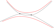
There are several difficulties for approximate parametrization of algebraic space curves. The first one is to preserve the topology of the algebraic space curve. In fact, there already exist some related work of computing the topology of algebraic space curves, reduced or non-reduced, for example [3, 16, 30, 24, 33]. Most of them require the curve to be in a generic position. For the space curves which are not in a generic position, one need to take a coordinate transformation such that the new space curve is in a generic position. Thus some geometric information of the original space curve is lost. Some non-singular critical points of the new space curve may not correspond to the non-singular critical points of the original space curve. One needs additional computation to get these points in the original coordinate system. Subdivision method can preserve the topology of the curve in a theoretical sense. But it is rather difficult to reach the required bound in practice currently [11, 32]. Even if one gets the topology of the given curve, the approximation curve may have different topology as the original curve when two or more curve segments are very close( see Figure 2). The second difficulty is the error control of the approximation curve. Some error functions is reliable but it is not easy to compute in practice, for example [15]. We need to find a reliable and efficient method to control the error during the approximation. The third one is the continuity of the approximation curve. We usually require the approximation to be C1superscript๐ถ1C^{1}(or G1superscript๐บ1G^{1})-continuous or higher in practice. Doing so, we need compute the tangent directions of algebraic space curve at some points. It is not a trivial task especially when the component considered is non-reduced. Its tangent direction can not be decided by the normal directions (โˆ‚fโˆ‚x,โˆ‚fโˆ‚y,โˆ‚fโˆ‚z)๐‘“๐‘ฅ๐‘“๐‘ฆ๐‘“๐‘ง(\frac{\partial f}{\partial x},\frac{\partial f}{\partial y},\frac{\partial f}{\partial z}), (โˆ‚gโˆ‚x,โˆ‚gโˆ‚y,โˆ‚gโˆ‚z)๐‘”๐‘ฅ๐‘”๐‘ฆ๐‘”๐‘ง(\frac{\partial g}{\partial x},\frac{\partial g}{\partial y},\frac{\partial g}{\partial z}) of the two surfaces f=0๐‘“0f=0 and g=0๐‘”0g=0 at the given point. In the non-reduced case, two normal directions are parallel or at least one of them does not exist at the point.

There exist nice work about approximating of algebraic space curves. Exact parametrization of the intersection of algebraic surfaces is obtained in [1, 10, 17, 18, 19, 22, 27, 39, 41, 43, 45]. Of course, it is topology preserving. The approximation of the intersection of generic algebraic surfaces with numeric method is also considered [5, 6, 31, 34, 36]. Usually, numeric method cannot guarantee the topology of the original algebraic space curve.

In [7], the authors considered approximating of the regular algebraic space curves with circular arcs by numeric method combining with the subdivision method. It works well for low degree algebraic space curves. In [23], the authors present an algorithm to approximate an irreducible space curves under a given precision. It based on the fact that there exists a birational map between the projection curve ๐’ž๐’ž{\mathcal{C}} for some direction and the irreducible algebraic space curve S๐‘†S. But an irreducible decomposition of a given two polynomials system is not an easy task. And we need to consider the intersection of two or more irreducible space curves after we decompose a reducible space curve. Other type of intersection problem of surfaces can be found in [34, 36] and related references.

In [10], the authors present an algorithm to approximate an algebraic space curve, defined by f=g=0๐‘“๐‘”0f=g=0, in the generic position with Fergusonโ€™s cubic ๐ฉโ€‹(t)=(xโ€‹(t),yโ€‹(t),zโ€‹(t)),tโˆˆ[0,1]formulae-sequence๐ฉ๐‘ก๐‘ฅ๐‘ก๐‘ฆ๐‘ก๐‘ง๐‘ก๐‘ก01\mathbf{p}(t)=(x(t),y(t),z(t)),t\in[0,1] and by minimizing an integral to control the error. They compute the topology of the space curve at first, so it is topology preserving. But they do not check whether the approximation curve exactly preserves the topology of the original space curve. And it works well for regular space curve. From the formula above, we can find that if some segments of the algebraic space curve is not regular, the method may fail.

In [37], the authors consider the irreducible algebraic space curve in generic position such that its projection is birational. They use a genus 0 plane algebraic curve to approximate the projection plane curve under a given precision if it exists. Thus they have a rational approximation space curve for the original space curve. The method is not topology preserving.

In this paper, we present a new algorithm to compute a certified G1superscript๐บ1G^{1} rational parametric approximation for algebraic space curves, which solves the three difficulties mentioned above nicely. The algorithm is certified in the sense that the approximation curve and the original curve have the same topology and their Hausdauff distance is smaller than a given precision. The algorithm works for algebraic space curves which need not to be regular or in generic positions. The key idea is to extend the local generic position method [13, 12] for zero-dimensional polynomial systems to one-dimensional algebraic space curves. The algorithm consists of four major steps.

Firstly, the space curve ๐’ฎ๐’ฎ{\mathcal{S}}, which is the intersection of fโ€‹(x,y,z)=0๐‘“๐‘ฅ๐‘ฆ๐‘ง0f(x,y,z)=0 and gโ€‹(x,y,z)=0๐‘”๐‘ฅ๐‘ฆ๐‘ง0g(x,y,z)=0, is projected to the xโ€‹y๐‘ฅ๐‘ฆxy-plane as a plane curve ๐’ž1subscript๐’ž1{\mathcal{C}}_{1} and ๐’ž1subscript๐’ž1{\mathcal{C}}_{1} is approximated piecewisely with functions of the form h1โ€‹(x),xโˆˆ[a,b]subscriptโ„Ž1๐‘ฅ๐‘ฅ๐‘Ž๐‘h_{1}(x),x\in[a,b].

Secondly, we find a number s>0๐‘ 0s>0 such that under the shear transformation ฯ†:(x,y,z)โ†’(x,y+sโ€‹z,z):๐œ‘โ†’๐‘ฅ๐‘ฆ๐‘ง๐‘ฅ๐‘ฆ๐‘ ๐‘ง๐‘ง\varphi:(x,y,z)\rightarrow(x,y+s\,z,z), ฯ†โ€‹(f)๐œ‘๐‘“\varphi(f) and ฯ†โ€‹(g)๐œ‘๐‘”\varphi(g) are in a generic position in the sense that there is a one to one correspondence between the curve segments of ๐’ฎ๐’ฎ{\mathcal{S}} and that of their projection curve ๐’ž2subscript๐’ž2{\mathcal{C}}_{2} to the xโ€‹y๐‘ฅ๐‘ฆxy-plane. The plane curve ๐’ž2subscript๐’ž2{\mathcal{C}}_{2} is also approximated piecewisely with functions of the form h2โ€‹(x),xโˆˆ[a,b]subscriptโ„Ž2๐‘ฅ๐‘ฅ๐‘Ž๐‘h_{2}(x),x\in[a,b].

Thirdly, we choose s๐‘ s such that ๐’ž2subscript๐’ž2{\mathcal{C}}_{2} is in a local generic position to ๐’ž1subscript๐’ž1{\mathcal{C}}_{1} in the following sense.

  • โ€ข

    The plane curves ๐’ž1subscript๐’ž1{\mathcal{C}}_{1} and ๐’ž2subscript๐’ž2{\mathcal{C}}_{2} can be divided into segments such that each segment of ๐’ž2subscript๐’ž2{\mathcal{C}}_{2} corresponds to a segment of ๐’ž1subscript๐’ž1{\mathcal{C}}_{1}.

  • โ€ข

    Let h1โ€‹(x),h2โ€‹(x),xโˆˆ[a,b]subscriptโ„Ž1๐‘ฅsubscriptโ„Ž2๐‘ฅ๐‘ฅ๐‘Ž๐‘h_{1}(x),h_{2}(x),x\in[a,b] be the approximations for a segment C1subscript๐ถ1C_{1} of ๐’ž1subscript๐’ž1{\mathcal{C}}_{1} and the corresponding curve segment C2subscript๐ถ2C_{2} of ๐’ž2subscript๐’ž2{\mathcal{C}}_{2} with precisions ฯต1subscriptitalic-ฯต1\epsilon_{1} and ฯต2subscriptitalic-ฯต2\epsilon_{2} respectively. Then the space curve segment S๐‘†S corresponding to C2subscript๐ถ2C_{2} can be approximated by (x,h1โ€‹(x),h2โ€‹(x)โˆ’h1โ€‹(x)s)๐‘ฅsubscriptโ„Ž1๐‘ฅsubscriptโ„Ž2๐‘ฅsubscriptโ„Ž1๐‘ฅ๐‘ (x,h_{1}(x),\frac{h_{2}(x)-h_{1}(x)}{s}) with precision s2โ€‹ฯต12+(ฯต1+ฯต2)2/ssuperscript๐‘ 2superscriptsubscriptitalic-ฯต12superscriptsubscriptitalic-ฯต1subscriptitalic-ฯต22๐‘ \sqrt{s^{2}\epsilon_{1}^{2}+(\epsilon_{1}+\epsilon_{2})^{2}}/s.

In other words, if ๐’ž2subscript๐’ž2{\mathcal{C}}_{2} is in a local generic position to ๐’ž1subscript๐’ž1{\mathcal{C}}_{1}, then each segment of the space curve can be represented as a linear combination of corresponding segments of ๐’ž1subscript๐’ž1{\mathcal{C}}_{1} and ๐’ž2subscript๐’ž2{\mathcal{C}}_{2}. As a consequence, a certified parametrization for the space curve can be computed from that of ๐’ž1subscript๐’ž1{\mathcal{C}}_{1} and ๐’ž2subscript๐’ž2{\mathcal{C}}_{2} directly. This step is the main contribution of the paper.

Finally, we show that a plane curve can be approximated such that the piecewise approximation curve for the space curve has G1superscript๐บ1G^{1} continuity and usually has the following forms: (x,aโ€‹x+b+cdโ€‹x+1,a1โ€‹x+b1+c1d1โ€‹x+1+c2d2โ€‹x+1)๐‘ฅ๐‘Ž๐‘ฅ๐‘๐‘๐‘‘๐‘ฅ1subscript๐‘Ž1๐‘ฅsubscript๐‘1subscript๐‘1subscript๐‘‘1๐‘ฅ1subscript๐‘2subscript๐‘‘2๐‘ฅ1(x,a\,x+b+\frac{c}{d\,x+1},a_{1}\,x+b_{1}+\frac{c_{1}}{d_{1}\,x+1}+\frac{c_{2}}{d_{2}\,x+1}), (aโ€‹y+b+cdโ€‹y+1,y,a1โ€‹y+b1+c1d1โ€‹y+1+c2d2โ€‹y+1)๐‘Ž๐‘ฆ๐‘๐‘๐‘‘๐‘ฆ1๐‘ฆsubscript๐‘Ž1๐‘ฆsubscript๐‘1subscript๐‘1subscript๐‘‘1๐‘ฆ1subscript๐‘2subscript๐‘‘2๐‘ฆ1(a\,y+b+\frac{c}{d\,y+1},y,a_{1}\,y+b_{1}+\frac{c_{1}}{d_{1}\,y+1}+\frac{c_{2}}{d_{2}\,y+1}).

The topology of the space curve is obtained directly from the two projection steps. Thus this new method can not only compute the topology of the space curve but approximate the algebraic space curve under any given precision.

The paper is organized as below. In the next section, we will consider the certified approximation of plane algebraic curve under a given precision. In Section 3, we will show the theory and algorithm for certified approximation of algebraic space curves. In Section 4, we will show some examples to illustrate the effectivity of our method. We draw a conclusion in the last section.

2 Approximate parametrization of plane algebraic curves

Given a plane algebraic curve defined by a square free polynomial fโˆˆโ„šโ€‹[x,y]๐‘“โ„š๐‘ฅ๐‘ฆf\in{\mathbb{Q}}[x,y], our aim is to give a piecewise C1superscript๐ถ1C^{1}-continuous approximation of ๐’ž={(x,y)โˆˆโ„2|fโ€‹(x,y)=0}๐’žconditional-set๐‘ฅ๐‘ฆsuperscriptโ„2๐‘“๐‘ฅ๐‘ฆ0{\mathcal{C}}=\{(x,y)\in{\mathbb{R}}^{2}|f(x,y)=0\} in a given box B={(x,y)โˆˆโ„2|aโ‰คxโ‰คb,cโ‰คyโ‰คd}๐ตconditional-set๐‘ฅ๐‘ฆsuperscriptโ„2formulae-sequence๐‘Ž๐‘ฅ๐‘๐‘๐‘ฆ๐‘‘B=\{(x,y)\in{\mathbb{R}}^{2}|a\leq x\leq b,c\leq y\leq d\} such that each piece of the approximation curve has the form (x,hโ€‹(x))๐‘ฅโ„Ž๐‘ฅ(x,h(x)) and the approximation error is bounded by a given precision ฯต>0italic-ฯต0\epsilon>0, where โ„š,โ„โ„šโ„{\mathbb{Q}},{\mathbb{R}} are the fields of rational numbers and real numbers, respectively. And the whole approximation curve has the same topology as ๐’ž๐’ž{\mathcal{C}}.

2.1 Notations

In this subsection, we will introduce some notations.

A point P=(x0,y0)๐‘ƒsubscript๐‘ฅ0subscript๐‘ฆ0P=(x_{0},y_{0}) is said to be a singular point on ๐’ž:fโ€‹(x,y)=0:๐’ž๐‘“๐‘ฅ๐‘ฆ0{\mathcal{C}}:f(x,y)=0 if fโ€‹(x0,y0)=fxโ€‹(x0,y0)=fyโ€‹(x0,y0)=0๐‘“subscript๐‘ฅ0subscript๐‘ฆ0subscript๐‘“๐‘ฅsubscript๐‘ฅ0subscript๐‘ฆ0subscript๐‘“๐‘ฆsubscript๐‘ฅ0subscript๐‘ฆ00f(x_{0},y_{0})=f_{x}(x_{0},y_{0})=f_{y}(x_{0},y_{0})=0, where fx=โˆ‚fโˆ‚x,fy=โˆ‚fโˆ‚yformulae-sequencesubscript๐‘“๐‘ฅ๐‘“๐‘ฅsubscript๐‘“๐‘ฆ๐‘“๐‘ฆf_{x}=\frac{\partial f}{\partial x},f_{y}=\frac{\partial f}{\partial y}. A non-singular point is called a regular point. An x๐‘ฅx-critical (A y๐‘ฆy-critical) point P=(x0,y0)๐‘ƒsubscript๐‘ฅ0subscript๐‘ฆ0P=(x_{0},y_{0}) is a point satisfying fโ€‹(x0,y0)=fyโ€‹(x0,y0)=0๐‘“subscript๐‘ฅ0subscript๐‘ฆ0subscript๐‘“๐‘ฆsubscript๐‘ฅ0subscript๐‘ฆ00f(x_{0},y_{0})=f_{y}(x_{0},y_{0})=0 (fโ€‹(x0,y0)=fxโ€‹(x0,y0)=0๐‘“subscript๐‘ฅ0subscript๐‘ฆ0subscript๐‘“๐‘ฅsubscript๐‘ฅ0subscript๐‘ฆ00f(x_{0},y_{0})=f_{x}(x_{0},y_{0})=0). So a singular point is both x๐‘ฅx-critical and y๐‘ฆy-critical points. The inflexion points or flexes of ๐’ž๐’ž{\mathcal{C}} are its non-singular points satisfying its Hession equation Hโ€‹(f)=0๐ป๐‘“0H(f)=0 (see [44]).

A regular curve segment C๐ถC of ๐’ž๐’ž{\mathcal{C}} is a connected part of ๐’ž๐’ž{\mathcal{C}} with two endpoints P0โ€‹(x0,y0)subscript๐‘ƒ0subscript๐‘ฅ0subscript๐‘ฆ0P_{0}(x_{0},y_{0}) and P1โ€‹(x1,y1)subscript๐‘ƒ1subscript๐‘ฅ1subscript๐‘ฆ1P_{1}(x_{1},y_{1}) (x0โ‰ x1subscript๐‘ฅ0subscript๐‘ฅ1x_{0}\neq x_{1}, both P0,P1subscript๐‘ƒ0subscript๐‘ƒ1P_{0},P_{1} are bounded) and there are no x๐‘ฅx-critical points, y๐‘ฆy-critical points, flex on C๐ถC except for P0,P1subscript๐‘ƒ0subscript๐‘ƒ1P_{0},P_{1}. So a regular curve segment is convex, monotonous w.r.t. x๐‘ฅx or y๐‘ฆy, and inside a triangle defined by its endpoints and their tangent directions. Let ฮ”ฮ”\Delta be the triangle defined by P0,P1subscript๐‘ƒ0subscript๐‘ƒ1P_{0},P_{1} and their tangent lines. An endpoint of a regular curve segment is called a vertical tangent point, VT point for short, if the regular curve segment has a vertical tangent line at this endpoint.

A parametric curve is said to be C1superscript๐ถ1C^{1}-continuous (G1superscript๐บ1G^{1}-continuous) if the curves are joined and the first derivatives are continuous (the curves also share a common tangent direction at the join point).

2.2 Curve segmentation of a real plane algebraic curve

In this subsection, we will show how to divide a plane curve inside a box B๐ตB, denoted as ๐’žBsubscript๐’ž๐ต{\mathcal{C}}_{B}, into regular curve segments with the form [P0โ€‹(x0,y0),P1โ€‹(x1,y1),T0โ€‹(1,k0),T1โ€‹(1,kโ€‹1)]subscript๐‘ƒ0subscript๐‘ฅ0subscript๐‘ฆ0subscript๐‘ƒ1subscript๐‘ฅ1subscript๐‘ฆ1subscript๐‘‡01subscript๐‘˜0subscript๐‘‡11๐‘˜1[P_{0}(x_{0},y_{0}),P_{1}(x_{1},y_{1}),T_{0}(1,k_{0}),T_{1}(1,k1)], where P0,P1subscript๐‘ƒ0subscript๐‘ƒ1P_{0},P_{1} are endpoints and T0,T1subscript๐‘‡0subscript๐‘‡1T_{0},T_{1} are tangent directions at the endpoints.

We will follow the steps below.

At first, Compute the topology of ๐’žBsubscript๐’ž๐ต{\mathcal{C}}_{B}. There are many related work to solve this problem, such as [2, 4, 8, 14, 20, 28, 38, 40]. Some methods work well, but they need a coordinate system transformation. We prefer the methods which do not take a coordinate system transformation.

Second, Compute all the flexes, x๐‘ฅx-critical and y๐‘ฆy-critical points of ๐’žBsubscript๐’ž๐ต{\mathcal{C}}_{B}. y๐‘ฆy-critical points are computed before. x๐‘ฅx-critical points and flexes can be obtained by solving the corresponding equations.

Third, we split the plane curve into regular curve segments at x๐‘ฅx(y๐‘ฆy)-critical points or flexes of ๐’žBsubscript๐’ž๐ต{\mathcal{C}}_{B}. An easy way to solve the problem is as follows. For all the x๐‘ฅx-coordinates of x๐‘ฅx-critical points and flexes, lifting them to split ๐’žBsubscript๐’ž๐ต{\mathcal{C}}_{B} at these intersection points. We can find all these endpoints.

Finally, we represent the tangent direction of any non-VT point as (1,k),kโˆˆโ„โˆ–{+โˆž,โˆ’โˆž}1๐‘˜๐‘˜โ„(1,k),k\in{\mathbb{R}}\setminus\{+\infty,-\infty\}. It is convenient for our approximation. The tangent direction of a VT point is defined to be (1,โˆž)1(1,\infty).
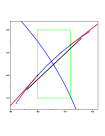
Tangent direction computation of singularities. We compute the tangent direction of a point close to a singularity on the regular curve segment to replace the tangent direction of the singularity. It is easy to compute. Let Pโ€‹(ฮฑ,ฮฒ)๐‘ƒ๐›ผ๐›ฝP(\alpha,\beta) be a singularity of a planar algebraic curve hโ€‹(x,y)=0โ„Ž๐‘ฅ๐‘ฆ0h(x,y)=0 and C:(x,y~โ€‹(x)),xโˆˆ[ฮฑ,ฮณ]:๐ถ๐‘ฅ~๐‘ฆ๐‘ฅ๐‘ฅ๐›ผ๐›พC:(x,\tilde{y}(x)),x\in[\alpha,\gamma] a regular curve segment originating from right side (left side is similar) of P๐‘ƒP. Then the tangent direction of C๐ถC at P๐‘ƒP is (1,t)=(1,limxโ†’ฮฑ+y~โ€‹(x)).1๐‘ก1subscriptโ†’๐‘ฅsuperscript๐›ผ~๐‘ฆ๐‘ฅ(1,t)=(1,\lim_{x\rightarrow\alpha^{+}}\tilde{y}(x)). In practice, we can take some point very close to P๐‘ƒP on C๐ถC, which is a regular point. Let [a,b]๐‘Ž๐‘[a,b] be the isolating interval of ฮฑ(โ‰ a,โ‰ b)\alpha(\neq a,\neq b). We can use the tangent direction of some regular point to replace the tangent direction of C๐ถC at P๐‘ƒP. For instance, (1,โˆ‚y~โ€‹(b)โˆ‚x)=(1,fxfy)1~๐‘ฆ๐‘๐‘ฅ1subscript๐‘“๐‘ฅsubscript๐‘“๐‘ฆ(1,\frac{\partial\tilde{y}(b)}{\partial x})=(1,\frac{f_{x}}{f_{y}}) can be regarded as the tangent direction of C๐ถC at P๐‘ƒP. For the regular curve segments shall the same tangent direction, we can take the average value of them as their tangent directions, and the center of the isolating box of P๐‘ƒP as the singularity, as shown in Figure 1. When C๐ถC has a vertical tangent direction, t=โˆž๐‘กt=\infty. If |โˆ‚y~โ€‹(b)โˆ‚x|>N~๐‘ฆ๐‘๐‘ฅ๐‘|\frac{\partial\tilde{y}(b)}{\partial x}|>N, for example, N=100๐‘100N=100, we can regard the regular curve segment have a vertical tangent direction.

If we cannot distinguish the tangent directions of two groups of regular curve segments, we can refine [a,b]๐‘Ž๐‘[a,b] to a narrower one and recompute the tangent directions again until we can distinguish them or they are less than some given bounded value ฯ„๐œ\tau such that |kโˆ’kโ€ฒ|<ฯ„๐‘˜superscript๐‘˜โ€ฒ๐œ|k-k^{\prime}|<\tau, where k,kโ€ฒ๐‘˜superscript๐‘˜โ€ฒk,k^{\prime} are tangent directions.

Refer to caption
Figure 1: Approximate the tangent direction of regular curve segments at a singularity
Refer to caption
Figure 2: The approximation curves change the topology of original ones

2.3 Approximation of a regular curve segment

We will give an approximate parametrization of real plane algebraic curves. Though Gao and Li [23] have obtained a rational quadratic approximation of real plane algebraic curves with B-splines, we need to derive a piecewise approximation curve as (x,hโ€‹(x))๐‘ฅโ„Ž๐‘ฅ(x,h(x)) of real plane algebraic curves in order to approximately parameterize real space algebraic curves in a different way. Let C๐ถC be the regular curve segment defined by two points P0โ€‹(x0,y0),P1โ€‹(x1,y1)subscript๐‘ƒ0subscript๐‘ฅ0subscript๐‘ฆ0subscript๐‘ƒ1subscript๐‘ฅ1subscript๐‘ฆ1P_{0}(x_{0},y_{0}),P_{1}(x_{1},y_{1}). We divide the approximation problem into two cases.

C๐ถC not containing a VT point. Given a regular curve segment C๐ถC, its two endpoints P0โ€‹(x0,y0),P1โ€‹(x1,y1)subscript๐‘ƒ0subscript๐‘ฅ0subscript๐‘ฆ0subscript๐‘ƒ1subscript๐‘ฅ1subscript๐‘ฆ1P_{0}(x_{0},y_{0}),P_{1}(x_{1},y_{1}) does not contain a VT point. And the tangent directions of the regular curve segment at P0,P1subscript๐‘ƒ0subscript๐‘ƒ1P_{0},P_{1} are (1,k0),(1,k1)1subscript๐‘˜01subscript๐‘˜1(1,k_{0}),(1,k_{1}), respectively. We will construct an explicit rational quadratic function Y1โ€‹(x)subscript๐‘Œ1๐‘ฅY_{1}(x) to approximate C๐ถC such that Y1โ€‹(xi)=yi,Y1โ€ฒโ€‹(xi)=ki,i=0,1formulae-sequencesubscript๐‘Œ1subscript๐‘ฅ๐‘–subscript๐‘ฆ๐‘–formulae-sequencesuperscriptsubscript๐‘Œ1โ€ฒsubscript๐‘ฅ๐‘–subscript๐‘˜๐‘–๐‘–01Y_{1}(x_{i})=y_{i},Y_{1}^{\prime}(x_{i})=k_{i},i=0,1, where Y1โ€ฒโ€‹(x)=โˆ‚Y1โˆ‚xโ€‹(x)superscriptsubscript๐‘Œ1โ€ฒ๐‘ฅsubscript๐‘Œ1๐‘ฅ๐‘ฅY_{1}^{\prime}(x)=\frac{\partial Y_{1}}{\partial x}(x).

Assuming that

Y1โ€‹(x)=aโ€‹x2+bโ€‹x+cdโ€‹x+1subscript๐‘Œ1๐‘ฅ๐‘Žsuperscript๐‘ฅ2๐‘๐‘ฅ๐‘๐‘‘๐‘ฅ1Y_{1}(x)=\frac{a\,x^{2}+b\,x+c}{d\,x+1} (1)

and x0=0,x1=1formulae-sequencesubscript๐‘ฅ00subscript๐‘ฅ11x_{0}=0,x_{1}=1, we have

Y1โ€‹(0)=y0,Y1โ€‹(1)=y1,Y1โ€ฒโ€‹(0)=k0,Y1โ€ฒโ€‹(1)=k1.formulae-sequencesubscript๐‘Œ10subscript๐‘ฆ0formulae-sequencesubscript๐‘Œ11subscript๐‘ฆ1formulae-sequencesuperscriptsubscript๐‘Œ1โ€ฒ0subscript๐‘˜0superscriptsubscript๐‘Œ1โ€ฒ1subscript๐‘˜1\displaystyle Y_{1}(0)=y_{0},Y_{1}(1)=y_{1},Y_{1}^{\prime}(0)=k_{0},Y_{1}^{\prime}(1)=k_{1}.

Solving a,b,c,d๐‘Ž๐‘๐‘๐‘‘a,b,c,d from the equations above, we have

a๐‘Ž\displaystyle a =\displaystyle= โˆ’2โ€‹y0โ€‹y1+y02โˆ’k0โ€‹k1+y12โˆ’y1+k1+y0,2subscript๐‘ฆ0subscript๐‘ฆ1superscriptsubscript๐‘ฆ02subscript๐‘˜0subscript๐‘˜1superscriptsubscript๐‘ฆ12subscript๐‘ฆ1subscript๐‘˜1subscript๐‘ฆ0\displaystyle{\frac{-2\,{\it y_{0}}\,{\it y_{1}}+{{\it y_{0}}}^{2}-{\it k_{0}}\,{\it k_{1}}+{{\it y_{1}}}^{2}}{-{\it y_{1}}+{\it k_{1}}+{\it y_{0}}}},
b๐‘\displaystyle b =\displaystyle= โˆ’โˆ’2โ€‹y0โ€‹y1+y0โ€‹k1+2โ€‹y02+k0โ€‹y1โˆ’k0โ€‹k1โˆ’y1+k1+y0,2subscript๐‘ฆ0subscript๐‘ฆ1subscript๐‘ฆ0subscript๐‘˜12superscriptsubscript๐‘ฆ02subscript๐‘˜0subscript๐‘ฆ1subscript๐‘˜0subscript๐‘˜1subscript๐‘ฆ1subscript๐‘˜1subscript๐‘ฆ0\displaystyle-{\frac{-2\,{\it y_{0}}\,{\it y_{1}}+{\it y_{0}}\,{\it k_{1}}+2\,{{\it y_{0}}}^{2}+{\it k_{0}}\,{\it y_{1}}-{\it k_{0}}\,{\it k_{1}}}{-{\it y_{1}}+{\it k_{1}}+{\it y_{0}}}},
c๐‘\displaystyle c =\displaystyle= y0,subscript๐‘ฆ0\displaystyle{\it y_{0}},
d๐‘‘\displaystyle d =\displaystyle= โˆ’โˆ’2โ€‹y1+k0+k1+2โ€‹y0โˆ’y1+k1+y0.2subscript๐‘ฆ1subscript๐‘˜0subscript๐‘˜12subscript๐‘ฆ0subscript๐‘ฆ1subscript๐‘˜1subscript๐‘ฆ0\displaystyle-{\frac{-2\,{\it y_{1}}+{\it k_{0}}+{\it k_{1}}+2\,{\it y_{0}}}{-{\it y_{1}}+{\it k_{1}}+{\it y_{0}}}}.

From the representation, we need to require

โˆ’y1+k1+y0โ‰ 0,subscript๐‘ฆ1subscript๐‘˜1subscript๐‘ฆ00-{\it y_{1}}+{\it k_{1}}+{\it y_{0}}\neq 0, (2)

and dโ€‹x+1๐‘‘๐‘ฅ1d\,x+1 has no roots in [0,1]01[0,1], that is, d>โˆ’1๐‘‘1d>-1, from which we can derive that

(โˆ’y1+k0+y0)โ€‹(โˆ’y1+k1+y0)<0.subscript๐‘ฆ1subscript๐‘˜0subscript๐‘ฆ0subscript๐‘ฆ1subscript๐‘˜1subscript๐‘ฆ00\left(-{\it y_{1}}+{\it k_{0}}+{\it y_{0}}\right)\left(-{\it y_{1}}+{\it k_{1}}+{\it y_{0}}\right)<0. (3)

From the mean value theorem, we know that y1โˆ’y0=kxsubscript๐‘ฆ1subscript๐‘ฆ0subscript๐‘˜๐‘ฅy_{1}-y_{0}=k_{x}, where kxsubscript๐‘˜๐‘ฅk_{x} is the tangent direction of some xโˆˆ(0,1)๐‘ฅ01x\in(0,1). Since C๐ถC is monotonous, so kxsubscript๐‘˜๐‘ฅk_{x} is some value between k0subscript๐‘˜0k_{0} and k1subscript๐‘˜1k_{1}. Thus conditions (2) and (3) are satisfied directly. We can easily transform the interval [0,1]01[0,1] to [x0,x1]subscript๐‘ฅ0subscript๐‘ฅ1[x_{0},x_{1}] by setting x=Xโˆ’x0x1โˆ’x0๐‘ฅ๐‘‹subscript๐‘ฅ0subscript๐‘ฅ1subscript๐‘ฅ0x=\frac{X-x_{0}}{x_{1}-x_{0}}, where xโˆˆ[0,1]๐‘ฅ01x\in[0,1] when Xโˆˆ[x0,x1]๐‘‹subscript๐‘ฅ0subscript๐‘ฅ1X\in[x_{0},x_{1}].

Furthermore, when dโ‰ 0๐‘‘0d\neq 0, that is to say โˆ’2โ€‹y1+k0+k1+2โ€‹y0โ‰ 02subscript๐‘ฆ1subscript๐‘˜0subscript๐‘˜12subscript๐‘ฆ00-2\,{\it y_{1}}+{\it k_{0}}+{\it k_{1}}+2\,{\it y_{0}}\neq 0. Then expression (1) can be transformed into

Y1โ€‹(x)=a~โ€‹x+b~+c~d~โ€‹x+1.subscript๐‘Œ1๐‘ฅ~๐‘Ž๐‘ฅ~๐‘~๐‘~๐‘‘๐‘ฅ1Y_{1}(x)=\tilde{a}\,x+\tilde{b}+\frac{\tilde{c}}{\tilde{d}\,x+1}. (4)

Though equation (4) is equivalent to equation (1) when dโ‰ 0๐‘‘0d\neq 0 essentially, it has a simpler form and can reduce computation when evaluation. When d=0๐‘‘0d=0, equation (1) is a polynomial of degree two. And we have simple expressions for parameters a,b,c๐‘Ž๐‘๐‘{\it a,b,c}, that is a=k1โˆ’k02๐‘Žsubscript๐‘˜1subscript๐‘˜02{\it a}=\frac{{\it k_{1}}-{\it k_{0}}}{2}, b=k0๐‘subscript๐‘˜0{\it b}=k_{0}, c=y0๐‘subscript๐‘ฆ0{\it c}=y_{0}.

C๐ถC containing a VT point. When a given regular curve segment contains a VT point, it means the tangent line at P0subscript๐‘ƒ0P_{0} or P1subscript๐‘ƒ1P_{1} is a vertical line xโˆ’x0=0๐‘ฅsubscript๐‘ฅ00x-x_{0}=0 or xโˆ’x1=0๐‘ฅsubscript๐‘ฅ10x-x_{1}=0. In this case, the method above does not work. But we can use part of an ellipse or a hyperbola (xโˆ’xo)2a2ยฑ(yโˆ’yo)2b2โˆ’1=0โ€‹(a>0,b>0)plus-or-minussuperscript๐‘ฅsubscript๐‘ฅ๐‘œ2superscript๐‘Ž2superscript๐‘ฆsubscript๐‘ฆ๐‘œ2superscript๐‘210formulae-sequence๐‘Ž0๐‘0\frac{(x-x_{o})^{2}}{a^{2}}\pm\frac{(y-y_{o})^{2}}{b^{2}}-1=0(a>0,b>0) to derive an approximate parametrization of a real plane algebraic curve. Note that a regular curve segment containing a VT point has four cases which exactly correspond to the four parts of an ellipse or a hyperbola: the vertical line is xโˆ’x0=0๐‘ฅsubscript๐‘ฅ00x-x_{0}=0 or xโˆ’x1=0๐‘ฅsubscript๐‘ฅ10x-x_{1}=0 and yโ‰ฅyo๐‘ฆsubscript๐‘ฆ๐‘œy\geq y_{o} or yโ‰คyo๐‘ฆsubscript๐‘ฆ๐‘œy\leq y_{o}. We consider the case that C๐ถC has a vertical tangent line at P0โ€‹(x0,y0)subscript๐‘ƒ0subscript๐‘ฅ0subscript๐‘ฆ0P_{0}(x_{0},y_{0}) and C๐ถC monotonously increases from P0subscript๐‘ƒ0P_{0} to P1subscript๐‘ƒ1P_{1}. And we assume that the tangent line at P1subscript๐‘ƒ1P_{1} is k1โ€‹(xโˆ’x1)โˆ’(yโˆ’y1)=0โ€‹(k1โ‰ฅ0)subscript๐‘˜1๐‘ฅsubscript๐‘ฅ1๐‘ฆsubscript๐‘ฆ10subscript๐‘˜10k_{1}(x-x_{1})-(y-y_{1})=0(k_{1}\geq 0). The approximate curve is Y2โ€‹(x)=yo+b|a2โˆ’(xโˆ’xo)2|aY_{2}(x)=y_{o}+\frac{b\sqrt{|a^{2}-(x-x_{o})^{2}}|}{a}. Note that we have xo=x0ยฑa,yo=y0formulae-sequencesubscript๐‘ฅ๐‘œplus-or-minussubscript๐‘ฅ0๐‘Žsubscript๐‘ฆ๐‘œsubscript๐‘ฆ0x_{o}=x_{0}\pm a,y_{o}=y_{0} from the property of the ellipse or the hyperbola. So we have

Y2โ€‹(x)=y0+b|a2โˆ’(xโˆ’x0โˆ’a)2|a.\displaystyle Y_{2}(x)=y_{0}+\frac{b\sqrt{|a^{2}-(x-x_{0}-a)^{2}}|}{a}. (5)

And Y2โ€‹(x1)=y1,Y2โ€ฒโ€‹(x1)=k1.formulae-sequencesubscript๐‘Œ2subscript๐‘ฅ1subscript๐‘ฆ1superscriptsubscript๐‘Œ2โ€ฒsubscript๐‘ฅ1subscript๐‘˜1Y_{2}(x_{1})=y_{1},Y_{2}^{\prime}(x_{1})=k_{1}. Solving it, we have

a๐‘Ž\displaystyle a =\displaystyle= (x1โˆ’x0)โ€‹(x0โ€‹k1+y1โˆ’y0โˆ’x1โ€‹k1)y1โˆ’y0โˆ’2โ€‹x1โ€‹k1+2โ€‹x0โ€‹k1,subscript๐‘ฅ1subscript๐‘ฅ0subscript๐‘ฅ0subscript๐‘˜1subscript๐‘ฆ1subscript๐‘ฆ0subscript๐‘ฅ1subscript๐‘˜1subscript๐‘ฆ1subscript๐‘ฆ02subscript๐‘ฅ1subscript๐‘˜12subscript๐‘ฅ0subscript๐‘˜1\displaystyle{\frac{\left({\it x_{1}}-{\it x_{0}}\right)\left({\it x_{0}}\,{\it k_{1}}+{\it y_{1}}-{\it y_{0}}-{\it x_{1}}\,{\it k_{1}}\right)}{{\it y_{1}}-{\it y_{0}}-2\,{\it x_{1}}\,{\it k_{1}}+2\,{\it x_{0}}\,{\it k_{1}}}},\,\,\,
b๐‘\displaystyle b =\displaystyle= (x0โ€‹k1+y1โˆ’y0โˆ’x1โ€‹k1)โ€‹y1โˆ’y0y1โˆ’y0โˆ’2โ€‹x1โ€‹k1+2โ€‹x0โ€‹k1.subscript๐‘ฅ0subscript๐‘˜1subscript๐‘ฆ1subscript๐‘ฆ0subscript๐‘ฅ1subscript๐‘˜1subscript๐‘ฆ1subscript๐‘ฆ0subscript๐‘ฆ1subscript๐‘ฆ02subscript๐‘ฅ1subscript๐‘˜12subscript๐‘ฅ0subscript๐‘˜1\displaystyle\left({\it x_{0}}\,{\it k_{1}}+{\it y_{1}}-{\it y_{0}}-{\it x_{1}}\,{\it k_{1}}\right)\sqrt{{\frac{{\it y_{1}}-{\it y_{0}}}{{\it y_{1}}-{\it y_{0}}-2\,{\it x_{1}}\,{\it k_{1}}+2\,{\it x_{0}}\,{\it k_{1}}}}}.

From the representation, we can find that a,b๐‘Ž๐‘a,b are well defined if k1<y1โˆ’y02โ€‹(x1โˆ’x0)subscript๐‘˜1subscript๐‘ฆ1subscript๐‘ฆ02subscript๐‘ฅ1subscript๐‘ฅ0k_{1}<\frac{y_{1}-y_{0}}{2\,(x_{1}-x_{0})} for an ellipse or k1>y1โˆ’y02โ€‹(x1โˆ’x0)subscript๐‘˜1subscript๐‘ฆ1subscript๐‘ฆ02subscript๐‘ฅ1subscript๐‘ฅ0k_{1}>\frac{y_{1}-y_{0}}{2\,(x_{1}-x_{0})} for a hyperbola. So we can choose (x1,y1)subscript๐‘ฅ1subscript๐‘ฆ1(x_{1},y_{1}) on the regular curve segment such that k1โ‰ y1โˆ’y02โ€‹(x1โˆ’x0)subscript๐‘˜1subscript๐‘ฆ1subscript๐‘ฆ02subscript๐‘ฅ1subscript๐‘ฅ0k_{1}\neq\frac{y_{1}-y_{0}}{2\,(x_{1}-x_{0})}. Then we can use part of an ellipse or a hyperbola to approximate the regular curve segments with VT points. The other three cases can be solved in a similar way.

Lemma 1

The two kinds of approximation curves above, say C~:(x,hโ€‹(x)),xโˆˆ[x0,x1]:~๐ถ๐‘ฅโ„Ž๐‘ฅ๐‘ฅsubscript๐‘ฅ0subscript๐‘ฅ1\tilde{C}:(x,h(x)),x\in[x_{0},x_{1}] for C๐ถC are inside the triangle formed by the endpoints and the tangent directions at the endpoints of C๐ถC, denoted as ฮ”ฮ”\Delta.

Proof. For both cases, C~~๐ถ\tilde{C} is part of a quadric curve. And the curve intersects all three edges of ฮ”ฮ”\Delta at least twice (including the multiplicities). If C~~๐ถ\tilde{C} goes out of ฮ”ฮ”\Delta, it will intersect the edge(s) at least three times (including multiplicities). But it is not possible since C~~๐ถ\tilde{C} is part of a quadric curve. So the lemma is true. โ–กโ–ก\Box

Topology preserving approximation. After we get the approximation regular curve segments, we need to check whether the approximation curve change the topology of the original curve. Even if we get the correct topology of the given algebraic planar curve, the approximation curve may have a different topology as the original curve, especially when two regular curve segments are very close, for example, see Figure 2. So we need to ensure that our numeric approximation curve has the same topology as the original one. We need only ensure that any two approximation curves, say C1,C2:(x,pโ€‹(x)),(x,qโ€‹(x)),xโˆˆ[a,b]:subscript๐ถ1subscript๐ถ2๐‘ฅ๐‘๐‘ฅ๐‘ฅ๐‘ž๐‘ฅ๐‘ฅ๐‘Ž๐‘C_{1},C_{2}:(x,p(x)),(x,q(x)),x\in[a,b], are disjoint. If pโ€‹(x)โˆ’qโ€‹(x)=0๐‘๐‘ฅ๐‘ž๐‘ฅ0p(x)-q(x)=0 has no real roots in (a,b)๐‘Ž๐‘(a,b), then the two approximation regular curve segments are disjoint. There are two kinds of approximation curves, say Y1โ€‹(x),Y2โ€‹(x)subscript๐‘Œ1๐‘ฅsubscript๐‘Œ2๐‘ฅY_{1}(x),Y_{2}(x). So we need to consider:
Case one: two approximation curves are both rational ones as Y1โ€‹(x)subscript๐‘Œ1๐‘ฅY_{1}(x). Then Tโ€‹(x)=pโ€‹(x)โˆ’qโ€‹(x)๐‘‡๐‘ฅ๐‘๐‘ฅ๐‘ž๐‘ฅT(x)=p(x)-q(x) can be simplified into a cubic univariate polynomial. It is easy to check whether it contains a real roots in (a,b)๐‘Ž๐‘(a,b) by its coefficients.
Case two: one is as Y1โ€‹(x)subscript๐‘Œ1๐‘ฅY_{1}(x) and the other is as Y2โ€‹(x)subscript๐‘Œ2๐‘ฅY_{2}(x). Then Tโ€‹(x)=pโ€‹(x)โˆ’qโ€‹(x)๐‘‡๐‘ฅ๐‘๐‘ฅ๐‘ž๐‘ฅT(x)=p(x)-q(x) can be simplified into a quartic univariate polynomial. It is also easy to check whether it contains a real roots in (a,b)๐‘Ž๐‘(a,b) by its coefficients.
Case three: both approximation curves are as Y2โ€‹(x)subscript๐‘Œ2๐‘ฅY_{2}(x). They both are parts of quadric algebraic curves. Considering the intersection of two quadric algebraic curves, we can judge whether C1,C2subscript๐ถ1subscript๐ถ2C_{1},C_{2} are disjoint or not.

Doing so as above, our approximation is exactly topology preserving.

2.4 Error control of the approximation

We will show the error control of the plane approximation curve in this subsection. In geometry, the approximation error should be defined as the following Hausdorff distance between the segment S๐‘†S and its approximation Sasubscript๐‘†๐‘ŽS_{a},

eโ€‹(S,Sa)=dโ€‹iโ€‹sโ€‹(S,Sa)=maxPโˆˆSโกminPโ€ฒโˆˆSaโกdโ€‹(P,Pโ€ฒ).๐‘’๐‘†subscript๐‘†๐‘Ž๐‘‘๐‘–๐‘ ๐‘†subscript๐‘†๐‘Žsubscript๐‘ƒ๐‘†subscriptsuperscript๐‘ƒโ€ฒsubscript๐‘†๐‘Ž๐‘‘๐‘ƒsuperscript๐‘ƒโ€ฒe(S,S_{a})=dis(S,S_{a})=\max_{P\in S}\min_{P^{\prime}\in S_{a}}d(P,P^{\prime}). (6)

However such a distance is difficult to compute. As an implement, the distance from an approximation parametric curve Pโ€‹(t)=(xโ€‹(t),yโ€‹(t)),0โ‰คtโ‰ค1formulae-sequence๐‘ƒ๐‘ก๐‘ฅ๐‘ก๐‘ฆ๐‘ก0๐‘ก1P(t)=(x(t),y(t)),0\leq t\leq 1 to the implicit defined curve ๐’ž:fโ€‹(x,y)=0:๐’ž๐‘“๐‘ฅ๐‘ฆ0{\mathcal{C}}:f(x,y)=0 is taken in the following form, which is called the error function [15],

eโ€‹(t)=fโ€‹(xโ€‹(t),yโ€‹(t))(fx(x(t),y(t))2+fy(x(t),y(t))2.e(t)=\frac{f(x(t),y(t))}{\sqrt{(f_{x}(x(t),y(t))^{2}+f_{y}(x(t),y(t))^{2}}}. (7)

The approximation error between Pโ€‹(t)๐‘ƒ๐‘กP(t) and ๐’ž๐’ž{\mathcal{C}} is set as an optimization problem

eโ€‹(Pโ€‹(t),๐’ž)=max0โ‰คtโ‰ค1โก(eโ€‹(t)).๐‘’๐‘ƒ๐‘ก๐’žsubscript0๐‘ก1๐‘’๐‘กe(P(t),{\mathcal{C}})=\max_{0\leq t\leq 1}(e(t)).

Let C:(x,y~โ€‹(x)),xโˆˆ[x0,x1]:๐ถ๐‘ฅ~๐‘ฆ๐‘ฅ๐‘ฅsubscript๐‘ฅ0subscript๐‘ฅ1C:(x,\tilde{y}(x)),x\in[x_{0},x_{1}] be the regular curve segment and Cยฏ:=(x,Yโ€‹(x)),xโˆˆ[x0,x1]formulae-sequenceassignยฏ๐ถ๐‘ฅ๐‘Œ๐‘ฅ๐‘ฅsubscript๐‘ฅ0subscript๐‘ฅ1\overline{C}:=(x,Y(x)),x\in[x_{0},x_{1}] its approximation curve. It is not difficult to find that the following bound is an upper bound of the Hausdorff distance between the segment C๐ถC and its approximation curve Cยฏยฏ๐ถ\overline{C} from (6):

maxxโˆˆ[x0,x1]โก|Yโ€‹(x)โˆ’y~โ€‹(x)|.subscript๐‘ฅsubscript๐‘ฅ0subscript๐‘ฅ1๐‘Œ๐‘ฅ~๐‘ฆ๐‘ฅ\max_{x\in[x_{0},x_{1}]}|Y(x)-\tilde{y}(x)|. (8)

We use Newton-Ralphson method to obtain y~โ€‹(xi0)~๐‘ฆsuperscriptsubscript๐‘ฅ๐‘–0\tilde{y}(x_{i}^{0}) at some point xi0โˆˆ[x0,x1]superscriptsubscript๐‘ฅ๐‘–0subscript๐‘ฅ0subscript๐‘ฅ1x_{i}^{0}\in[x_{0},x_{1}] in practice and Yโ€‹(xi0)๐‘Œsuperscriptsubscript๐‘ฅ๐‘–0Y(x_{i}^{0}) is the start point. If we fail to get a point with Newton-Ralphson method or the point satisfying |Yโ€‹(xi0)โˆ’y~โ€‹(xi0)|โ‰ฅฮด๐‘Œsuperscriptsubscript๐‘ฅ๐‘–0~๐‘ฆsuperscriptsubscript๐‘ฅ๐‘–0๐›ฟ|Y(x_{i}^{0})-\tilde{y}(x_{i}^{0})|\geq\delta, we can divide the regular curve segment into two ones. The approximation error is bounded by maxiโก{|Yโ€‹(xi0)โˆ’y~โ€‹(xi0)|}subscript๐‘–๐‘Œsuperscriptsubscript๐‘ฅ๐‘–0~๐‘ฆsuperscriptsubscript๐‘ฅ๐‘–0\max_{i}\{|Y(x_{i}^{0})-\tilde{y}(x_{i}^{0})|\}. In practice, we sample xi0superscriptsubscript๐‘ฅ๐‘–0x_{i}^{0} as xi0=x0+i/nโ€‹(x1โˆ’x0),0โ‰คiโ‰คnformulae-sequencesuperscriptsubscript๐‘ฅ๐‘–0subscript๐‘ฅ0๐‘–๐‘›subscript๐‘ฅ1subscript๐‘ฅ00๐‘–๐‘›x_{i}^{0}=x_{0}+i/n\,(x_{1}-x_{0}),0\leq i\leq n, for a proper value of n๐‘›n.

In order to control the error under a given precision, we need to divide the regular curve segment into two or more regular curve segments recursively until the error requirement satisfied. We subdivide the regular curve segments into two or more regular curve segments uniformly in the x๐‘ฅx coordinate. For any regular curve segment C:(x,y~โ€‹(x)),xโˆˆ[a,b]:๐ถ๐‘ฅ~๐‘ฆ๐‘ฅ๐‘ฅ๐‘Ž๐‘C:(x,\tilde{y}(x)),x\in[a,b], we denote the endpoints as P0โ€‹(x0,y0),P1โ€‹(x1,y1)subscript๐‘ƒ0subscript๐‘ฅ0subscript๐‘ฆ0subscript๐‘ƒ1subscript๐‘ฅ1subscript๐‘ฆ1P_{0}(x_{0},y_{0}),P_{1}(x_{1},y_{1}) and the tangent directions as (1,ki),i=0,1formulae-sequence1subscript๐‘˜๐‘–๐‘–01(1,k_{i}),i=0,1. We can find that P0,P1subscript๐‘ƒ0subscript๐‘ƒ1P_{0},P_{1} and two tangent directions form a triangle. One can subdivide the regular curve segment into two (or more) ones, for example, C1:xโˆˆ[x0,(x0+x1)/2],C2:xโˆˆ[(x0+x1)/2,x1]:subscript๐ถ1๐‘ฅsubscript๐‘ฅ0subscript๐‘ฅ0subscript๐‘ฅ12subscript๐ถ2:๐‘ฅsubscript๐‘ฅ0subscript๐‘ฅ12subscript๐‘ฅ1C_{1}:x\in[x_{0},(x_{0}+x_{1})/2],C_{2}:x\in[(x_{0}+x_{1})/2,x_{1}], if the precision is not satisfied. For the approximation curve of our method, we will prove that it can achieve any given precision.

Theorem 2

Let P0,P1subscript๐‘ƒ0subscript๐‘ƒ1P_{0},P_{1} be the endpoints of a regular curve segment C๐ถC and ฮ”ฮ”\Delta the triangle related to the regular curve segment as defined before. The Hausdorff distance between C๐ถC and its approximation curve(s) tends to zero if we subdivide C๐ถC into two or more regular curve segments recursively.

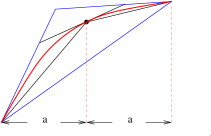
Proof. We will consider divide C๐ถC into two regular curve segments for the proof since dividing them into more regular curve segments are similar. Let Pโ€‹((x0+x1)/2,yยฏ)๐‘ƒsubscript๐‘ฅ0subscript๐‘ฅ12ยฏ๐‘ฆP((x_{0}+x_{1})/2,\bar{y}) be a point on C๐ถC. Denote the triangles formed by P1,Pโ€‹(P,P2)subscript๐‘ƒ1๐‘ƒ๐‘ƒsubscript๐‘ƒ2P_{1},P(P,P_{2}) and the tangent directions of C๐ถC at these points as ฮ”1โ€‹(ฮ”2)subscriptฮ”1subscriptฮ”2\Delta_{1}(\Delta_{2}). Let the lengths of the line segments P1โ€‹Pยฏ,Pโ€‹P2ยฏยฏsubscript๐‘ƒ1๐‘ƒยฏ๐‘ƒsubscript๐‘ƒ2\overline{P_{1}P},\overline{PP_{2}} be L11,L21superscriptsubscript๐ฟ11superscriptsubscript๐ฟ21L_{1}^{1},L_{2}^{1} and the heights of the triangles ฮ”1,ฮ”2subscriptฮ”1subscriptฮ”2\Delta_{1},\Delta_{2} corresponding to the edges P1โ€‹Pยฏ,Pโ€‹P2ยฏยฏsubscript๐‘ƒ1๐‘ƒยฏ๐‘ƒsubscript๐‘ƒ2\overline{P_{1}P},\overline{PP_{2}} are H11,H21superscriptsubscript๐ป11superscriptsubscript๐ป21H_{1}^{1},H_{2}^{1}, as shown in Figure 3. Subdividing the regular curve segments recursively in a similar way, denoting the length of the edges and heights as Lji,Hjisuperscriptsubscript๐ฟ๐‘—๐‘–superscriptsubscript๐ป๐‘—๐‘–L_{j}^{i},H_{j}^{i} of the triangles, we have the sum of the areas of these triangles are

A=โˆ‘j(Ljiโ€‹Hji/2)<12โ€‹โˆ‘jLjiโ€‹maxjโกHji.๐ดsubscript๐‘—superscriptsubscript๐ฟ๐‘—๐‘–superscriptsubscript๐ป๐‘—๐‘–212subscript๐‘—superscriptsubscript๐ฟ๐‘—๐‘–subscript๐‘—superscriptsubscript๐ป๐‘—๐‘–A=\sum_{j}(L_{j}^{i}\,H_{j}^{i}/2)<\frac{1}{2}\sum_{j}L_{j}^{i}\max_{j}H_{j}^{i}.

Assume that one edge Lji=P1โ€ฒโ€‹P2โ€ฒยฏ,P1โ€ฒโ€‹(x1โ€ฒ,y1โ€ฒ),P2โ€ฒโ€‹(x2โ€ฒ,y2โ€ฒ)superscriptsubscript๐ฟ๐‘—๐‘–ยฏsuperscriptsubscript๐‘ƒ1โ€ฒsuperscriptsubscript๐‘ƒ2โ€ฒsuperscriptsubscript๐‘ƒ1โ€ฒsuperscriptsubscript๐‘ฅ1โ€ฒsuperscriptsubscript๐‘ฆ1โ€ฒsuperscriptsubscript๐‘ƒ2โ€ฒsuperscriptsubscript๐‘ฅ2โ€ฒsuperscriptsubscript๐‘ฆ2โ€ฒL_{j}^{i}=\overline{P_{1}^{\prime}P_{2}^{\prime}},P_{1}^{\prime}(x_{1}^{\prime},y_{1}^{\prime}),P_{2}^{\prime}(x_{2}^{\prime},y_{2}^{\prime}). Since the given regular curve segment is bounded, |y2โ€ฒโˆ’y1โ€ฒ|superscriptsubscript๐‘ฆ2โ€ฒsuperscriptsubscript๐‘ฆ1โ€ฒ|y_{2}^{\prime}-y_{1}^{\prime}| tends to zero when |x2โ€ฒโˆ’x1โ€ฒ|superscriptsubscript๐‘ฅ2โ€ฒsuperscriptsubscript๐‘ฅ1โ€ฒ|x_{2}^{\prime}-x_{1}^{\prime}| tends to zero. And โˆ‘jLjisubscript๐‘—superscriptsubscript๐ฟ๐‘—๐‘–\sum_{j}L_{j}^{i} tends to the length of arc, say โ„’โ„’\mathcal{L}, of the given regular curve segment and Hjisuperscriptsubscript๐ป๐‘—๐‘–H_{j}^{i} tends to zero when all corresponding |x2โ€ฒโˆ’x1โ€ฒ|superscriptsubscript๐‘ฅ2โ€ฒsuperscriptsubscript๐‘ฅ1โ€ฒ|x_{2}^{\prime}-x_{1}^{\prime}| of Ljisuperscriptsubscript๐ฟ๐‘—๐‘–L_{j}^{i} tends to zero. Thus A๐ดA tends to zero. From the result of Lemma 1, we can have the opinion that we have a proof of the theorem. โ–กโ–ก\Box

There are two ways to find the subdivision points on a given regular curve segment C:(x,y~โ€‹(x)),xโˆˆ[a,b]:๐ถ๐‘ฅ~๐‘ฆ๐‘ฅ๐‘ฅ๐‘Ž๐‘C:(x,\tilde{y}(x)),x\in[a,b]. Since we get the topology of the plane projection curve, we know the order of the given regular curve segment among all the regular curve segments of the projection curve hโ€‹(x,y)=0โ„Ž๐‘ฅ๐‘ฆ0h(x,y)=0 when x๐‘ฅx changes from a๐‘Ža to b๐‘b. That is, we can find the point on C๐ถC for a fixed x๐‘ฅx coordinate, say x0โˆˆ(a,b)subscript๐‘ฅ0๐‘Ž๐‘x_{0}\in(a,b). It is the real root with the same order of hโ€‹(x0,y)=0โ„Žsubscript๐‘ฅ0๐‘ฆ0h(x_{0},y)=0 in a fixed interval (or (โˆ’โˆž,+โˆž)(-\infty,+\infty)).

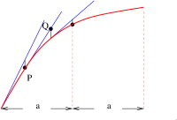
Another way is a local method. We can trace the regular curve segment to find the point on C๐ถC with given x๐‘ฅx coordinate since the regular curve segments are monotonous and convex. From the endpoint of the regular curve segment, compute the tangent line of the regular curve segment at some point P๐‘ƒP, find a point Q๐‘„Q on the tangent line by increasing the x๐‘ฅx coordinate such that the line segment Pโ€‹Qยฏยฏ๐‘ƒ๐‘„\overline{PQ} has no intersection with the projection curve. Then fix the x๐‘ฅx coordinate of Q๐‘„Q, to find a point on the regular curve segment. Note that we know the direction to find the point from the positiveness or negativeness of the tangent direction. Doing so recursively, we can find the point that we want, as shown in Figure 4.
Refer to caption
Figure 3: Splitting a regular curve segment
Refer to caption
Figure 4: Finding subdivision point by tracing

With the preparation above, we have the following algorithm to approximate a plane algebraic curve.

Algorithm 3

The inputs are ๐’ž:fโ€‹(x,y)=0:๐’ž๐‘“๐‘ฅ๐‘ฆ0{\mathcal{C}}:f(x,y)=0, a bounding box B๐ตB and an error bound ฮด>0๐›ฟ0\delta>0. The outputs are parametric curves ๐’ž1:={Bi(x)=(x,yi(x)),aiโ‰คxโ‰คbi,(i=1,โ€ฆ,N)}{\mathcal{C}}_{1}:=\{B_{i}(x)=(x,y_{i}(x)),a_{i}\leq x\leq b_{i},(i=1,...,N)\}, such that they give a C1superscript๐ถ1C^{1}-continuous and topology preserving approximation to ๐’žBsubscript๐’ž๐ต{\mathcal{C}}_{B} with eโ€‹(๐’ž1,๐’ž)<ฮด๐‘’subscript๐’ž1๐’ž๐›ฟe({\mathcal{C}}_{1},{\mathcal{C}})<\delta.

  1. 1.

    Regular curve segmentation of ๐’žBsubscript๐’ž๐ต{\mathcal{C}}_{B} as in Section 2.2.

  2. 2.

    Regular curve segment approximation as in Section 2.3 with error control of the approximation as in Section 2.4.

The correctness of the algorithm is clear from the analysis above. The termination of the algorithm is guaranteed by Lemma 1 and Theorem 2.

3 Certified approximate parametrization of algebraic space curves

In this section, we will consider approximate parametrization of algebraic space curves defined by f,gโˆˆโ„šโ€‹[x,y,z]๐‘“๐‘”โ„š๐‘ฅ๐‘ฆ๐‘งf,g\in{\mathbb{Q}}[x,y,z] such that two assumptions hold:

  • โ€ข

    For any x0โˆˆโ„subscript๐‘ฅ0โ„x_{0}\in{\mathbb{R}}, fโ€‹(x0,y,z)=gโ€‹(x0,y,z)=0๐‘“subscript๐‘ฅ0๐‘ฆ๐‘ง๐‘”subscript๐‘ฅ0๐‘ฆ๐‘ง0f(x_{0},y,z)=g(x_{0},y,z)=0 has a finite number of solutions; and

  • โ€ข

    the leading coefficients of f,g๐‘“๐‘”f,g w.r.t. z๐‘งz have no common factors only in x๐‘ฅx.

The assumptions are to ensure that we can use local generic position method to recover the points on the space curve from the points on two plane projection curves. The first assumption ensures that the algebraic space curve defined by f=g=0๐‘“๐‘”0f=g=0 does not have a plane curve on the plane x=x0๐‘ฅsubscript๐‘ฅ0x=x_{0}. The second assumption ensures that we can find a generic position only by taking a shear map (x,y,z)โ†’(x,y+sโ€‹z,z)โ†’๐‘ฅ๐‘ฆ๐‘ง๐‘ฅ๐‘ฆ๐‘ ๐‘ง๐‘ง(x,y,z)\rightarrow(x,y+s\,z,z). If the two projection curves have no factors only involving x๐‘ฅx, the two assumptions hold.

In fact, most of the problems we considered satisfy the condition. Note that we can exchange x,y,z๐‘ฅ๐‘ฆ๐‘งx,y,z freely. And another coordinate system transformation (x,y,z)โ†’(x+sโ€‹z,y,z)โ†’๐‘ฅ๐‘ฆ๐‘ง๐‘ฅ๐‘ ๐‘ง๐‘ฆ๐‘ง(x,y,z)\rightarrow(x+s\,z,y,z) can help us to find out the missing regular curve segments in the first transformation, even when the algebraic space curve containing vertical lines. Thus we can remove the assumptions with the method mentioned here. But we still assume the two assumptions holds in this section.

3.1 Definition of local generic position

In order to reduce the 3D approximation of space curves into 2D approximation of plane curves, we need the concept of local generic position. We recall the related definitions for zero-dimensional bivariate polynomial system [12]. Let โ„‚โ„‚{\mathbb{C}} be the field of complex numbers. Let f,gโˆˆโ„šโ€‹[x,y]๐‘“๐‘”โ„š๐‘ฅ๐‘ฆf,g\in{\mathbb{Q}}[x,y].

Refer to caption
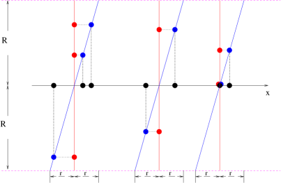
Figure 5: LGP method

We say two plane curves defined by two polynomials f,g๐‘“๐‘”f,g such that gcdโก(f,g)=1๐‘“๐‘”1\gcd(f,g)=1 are in a generic position w.r.t. y๐‘ฆy if
1) The leading coefficients of f๐‘“f and g๐‘”g w.r.t. y๐‘ฆy have no common factors.
2) Let hโ„Žh be the resultant of f๐‘“f and g๐‘”g w.r.t. y๐‘ฆy. For any ฮฑโˆˆโ„‚๐›ผโ„‚\alpha\in{\mathbb{C}} such that hโ€‹(ฮฑ)=0โ„Ž๐›ผ0h(\alpha)=0, fโ€‹(ฮฑ,y),gโ€‹(ฮฑ,y)๐‘“๐›ผ๐‘ฆ๐‘”๐›ผ๐‘ฆf(\alpha,y),g(\alpha,y) have only one common zero in โ„‚โ„‚{\mathbb{C}}.

Then we will introduce the technique of local generic position (LGP for short) method.

Given f,gโˆˆโ„šโ€‹[x,y]๐‘“๐‘”โ„š๐‘ฅ๐‘ฆf,g\in{\mathbb{Q}}[x,y], not necessarily to be in generic position, we can take a coordinate system transformation ฯ•:(x,y)โ†’(x+sโ€‹y,y),sโˆˆโ„š:italic-ฯ•formulae-sequenceโ†’๐‘ฅ๐‘ฆ๐‘ฅ๐‘ ๐‘ฆ๐‘ฆ๐‘ โ„š\phi:(x,y)\rightarrow(x+s\,y,y),s\in{\mathbb{Q}} such that

  • โ€ข

    ฯ•โ€‹(f),ฯ•โ€‹(g)italic-ฯ•๐‘“italic-ฯ•๐‘”\phi(f),\phi(g) are in a generic position w.r.t. x๐‘ฅx.

  • โ€ข

    Let hยฏยฏโ„Ž\bar{h}, hโ„Žh be the resultants of ฯ•โ€‹(f),ฯ•โ€‹(g)italic-ฯ•๐‘“italic-ฯ•๐‘”\phi(f),\phi(g) and f,g๐‘“๐‘”f,g w.r.t. y๐‘ฆy, respectively. Each root ฮฑ๐›ผ\alpha of hโ€‹(x)=0โ„Ž๐‘ฅ0h(x)=0 has a neighbor interval Hฮฑsubscript๐ป๐›ผH_{\alpha} such that HฮฑโˆฉHฮฒ=โˆ…subscript๐ป๐›ผsubscript๐ป๐›ฝH_{\alpha}\cap H_{\beta}=\emptyset for roots ฮฒโ‰ ฮฑ๐›ฝ๐›ผ\beta\neq\alpha of h=0โ„Ž0h=0. And any root (ฮณ,ฮท)๐›พ๐œ‚(\gamma,\eta) of f=g=0๐‘“๐‘”0f=g=0 which has a same x๐‘ฅx-coordinate ฮณ๐›พ\gamma, is mapped to ฮณโ€ฒ=ฮณ+sโ€‹ฮทโˆˆHฮณsuperscript๐›พโ€ฒ๐›พ๐‘ ๐œ‚subscript๐ป๐›พ\gamma^{\prime}=\gamma+s\,\eta\in H_{\gamma}, where hโ€‹(ฮณ)=0,hยฏโ€‹(ฮณโ€ฒ)=0formulae-sequenceโ„Ž๐›พ0ยฏโ„Žsuperscript๐›พโ€ฒ0h(\gamma)=0,\bar{h}(\gamma^{\prime})=0, as shown in Figure 5. Thus we can recover ฮท=ฮณโ€ฒโˆ’ฮณs๐œ‚superscript๐›พโ€ฒ๐›พ๐‘ \eta=\frac{\gamma^{\prime}-\gamma}{s}.

We can find the method has two nice properties: 1) The 2D solving problem is transformed into a 1D solving problem. 2) The error control of the solutions is easier.

3.2 Basic idea

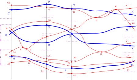
Now we want to extend this technique to 3-D case. Let fโˆงg๐‘“๐‘”f\wedge g denote the algebraic space curve defined by f=g=0๐‘“๐‘”0f=g=0. Denote ฯ€z:(x,y,z)โ†’(x,y):subscript๐œ‹๐‘งโ†’๐‘ฅ๐‘ฆ๐‘ง๐‘ฅ๐‘ฆ\pi_{z}:(x,y,z)\rightarrow(x,y) and h=ฯ€zโ€‹(fโˆงg)โ„Žsubscript๐œ‹๐‘ง๐‘“๐‘”h=\pi_{z}(f\wedge g). Let ฯ†:(x,y,z)โ†’(x,y+sโ€‹z,z):๐œ‘โ†’๐‘ฅ๐‘ฆ๐‘ง๐‘ฅ๐‘ฆ๐‘ ๐‘ง๐‘ง\varphi:(x,y,z)\rightarrow(x,y+s\,z,z), hยฏ=ฯ€zโ€‹(ฯ†โ€‹(f)โˆงฯ†โ€‹(g))ยฏโ„Žsubscript๐œ‹๐‘ง๐œ‘๐‘“๐œ‘๐‘”\bar{h}=\pi_{z}(\varphi(f)\wedge\varphi(g)). For a proper regular curve segment C:(x,pโ€‹(x)),xโˆˆ[x0,x1]:๐ถ๐‘ฅ๐‘๐‘ฅ๐‘ฅsubscript๐‘ฅ0subscript๐‘ฅ1C:(x,p(x)),x\in[x_{0},x_{1}] of the plane curve defined by h=0โ„Ž0h=0, it corresponds to one (the corresponding space regular curve segment may be at infinity) or more space regular curve segment(s), denoted as S1,โ€ฆ,Stsubscript๐‘†1โ€ฆsubscript๐‘†๐‘กS_{1},\ldots,S_{t}. If we can choose a proper s๐‘ s such that ฯ†โ€‹(f),ฯ†โ€‹(g)๐œ‘๐‘“๐œ‘๐‘”\varphi(f),\varphi(g) is in โ€œa goodโ€ position, and it has some local property, that is, the corresponding projection regular curve segments of S1,โ€ฆ,Stsubscript๐‘†1โ€ฆsubscript๐‘†๐‘กS_{1},\ldots,S_{t}, say Ci:(x,qiโ€‹(x)),xโˆˆ[x0,x1]โ€‹(i=1,โ€ฆ,t):subscript๐ถ๐‘–๐‘ฅsubscript๐‘ž๐‘–๐‘ฅ๐‘ฅsubscript๐‘ฅ0subscript๐‘ฅ1๐‘–1โ€ฆ๐‘กC_{i}:(x,q_{i}(x)),x\in[x_{0},x_{1}](i=1,\ldots,t), are in a fixed neighborhood of C๐ถC, then we can recover the z๐‘งz-coordinate of Si:z=qiโ€‹(x)โˆ’pโ€‹(x)sโ€‹(i=1,โ€ฆ,t):subscript๐‘†๐‘–๐‘งsubscript๐‘ž๐‘–๐‘ฅ๐‘๐‘ฅ๐‘ ๐‘–1โ€ฆ๐‘กS_{i}:z=\frac{q_{i}(x)-p(x)}{s}(i=1,\ldots,t). But to make Cisubscript๐ถ๐‘–C_{i} in a fixed neighborhood of C๐ถC is an unreachable task sometimes. Fortunately, what we need is to find out the correspondence between the regular curve segments of the plane curves defined by h=0โ„Ž0h=0 and hยฏ=0ยฏโ„Ž0\bar{h}=0. We can choose some sample points on x๐‘ฅx-axis, say xi(0),i=1,โ€ฆ,nformulae-sequencesuperscriptsubscript๐‘ฅ๐‘–0๐‘–1โ€ฆ๐‘›x_{i}^{(0)},i=1,\ldots,n, a proper s๐‘ s such that ฯ†โ€‹(fโ€‹(xi(0),y,z)),ฯ†โ€‹(gโ€‹(xi(0),y,z))๐œ‘๐‘“superscriptsubscript๐‘ฅ๐‘–0๐‘ฆ๐‘ง๐œ‘๐‘”superscriptsubscript๐‘ฅ๐‘–0๐‘ฆ๐‘ง\varphi(f(x_{i}^{(0)},y,z)),\varphi(g(x_{i}^{(0)},y,z)) are in a generic position. Then we can figure out the correspondence between the regular curve segments of h=0โ„Ž0h=0 and hยฏ=0ยฏโ„Ž0\bar{h}=0, as shown in Figure 6.

To realize the aim above, there are two key steps. One is how to find an approximation s๐‘ s, the other is how to find the correspondence between the regular curve segments of h=0โ„Ž0h=0 and hยฏ=0ยฏโ„Ž0\bar{h}=0. We need some preparations at first.

We say that two algebraic surfaces defined by f,gโˆˆโ„šโ€‹[x,y,z]๐‘“๐‘”โ„š๐‘ฅ๐‘ฆ๐‘งf,g\in{\mathbb{Q}}[x,y,z] such that gcdโก(f,g)=1๐‘“๐‘”1\gcd(f,g)=1 are in a z๐‘งz-generic position if
1) The leading coefficients of f๐‘“f and g๐‘”g w.r.t. z๐‘งz have no common factors.
2) Let hโ„Žh be the resultant of f๐‘“f and g๐‘”g w.r.t. z๐‘งz. There are only a finite number of zeros (ฮฑ,ฮฒ)โˆˆโ„‚2๐›ผ๐›ฝsuperscriptโ„‚2(\alpha,\beta)\in{\mathbb{C}}^{2} such that (ฮฑ,ฮฒ)๐›ผ๐›ฝ(\alpha,\beta) is not a y๐‘ฆy-critical point, hโ€‹(ฮฑ,ฮฒ)=0โ„Ž๐›ผ๐›ฝ0h(\alpha,\beta)=0 and fโ€‹(ฮฑ,ฮฒ,z),gโ€‹(ฮฑ,ฮฒ,z)๐‘“๐›ผ๐›ฝ๐‘ง๐‘”๐›ผ๐›ฝ๐‘งf(\alpha,\beta,z),g(\alpha,\beta,z) have more than one distinct common zeros in โ„‚โ„‚{\mathbb{C}}.

The definition is similar to the definition of pseudo-generic position in [16]. In Theorem 4 of [16], the authors also provide a method to check whether two given surfaces are in a pseudo-generic position or not.

Computing s๐‘ s. We will show how to find an s๐‘ s mentioned before. Let ฯ€y:(x,y)โ†’(x):subscript๐œ‹๐‘ฆโ†’๐‘ฅ๐‘ฆ๐‘ฅ\pi_{y}:(x,y)\rightarrow(x). Denote the real roots of ฯ€yโ€‹(h)=0subscript๐œ‹๐‘ฆโ„Ž0\pi_{y}(h)=0 and the x๐‘ฅx-coordinates of the flexes and x๐‘ฅx-critical points of h=0โ„Ž0h=0 as ฮฑ1,ฮฑ3,โ€ฆ,ฮฑ2โ€‹tโˆ’1subscript๐›ผ1subscript๐›ผ3โ€ฆsubscript๐›ผ2๐‘ก1\alpha_{1},\alpha_{3},\ldots,\alpha_{2\,t-1}. Find two rational numbers less than ฮฑ1subscript๐›ผ1\alpha_{1} and larger than ฮฑ2โ€‹tโˆ’1subscript๐›ผ2๐‘ก1\alpha_{2\,t-1}, denoted as ฮฑ0,ฮฑ2โ€‹tsubscript๐›ผ0subscript๐›ผ2๐‘ก\alpha_{0},\alpha_{2\,t} respectively. For any two adjacent real roots ฮฑ2โ€‹iโˆ’1,ฮฑ2โ€‹i+1subscript๐›ผ2๐‘–1subscript๐›ผ2๐‘–1\alpha_{2\,i-1},\alpha_{2\,i+1} of ฯ€yโ€‹(h)=0subscript๐œ‹๐‘ฆโ„Ž0\pi_{y}(h)=0, we can find a rational number, say ฮฑ2โ€‹isubscript๐›ผ2๐‘–\alpha_{2\,i}. Then we obtain a sequence ฮฑiโ€‹(i=0,โ€ฆ,2โ€‹t)subscript๐›ผ๐‘–๐‘–0โ€ฆ2๐‘ก\alpha_{i}(i=0,\ldots,2\,t). Assume the real roots of hโ€‹(ฮฑi,y)=0โ„Žsubscript๐›ผ๐‘–๐‘ฆ0h(\alpha_{i},y)=0 are ฮฒi,jโ€‹(j=0,โ€ฆ,ti)subscript๐›ฝ๐‘–๐‘—๐‘—0โ€ฆsubscript๐‘ก๐‘–\beta_{i,j}(j=0,\ldots,t_{i}) which are listed in increasing order. We can find out that (ฮฑi,ฮฒi,j)subscript๐›ผ๐‘–subscript๐›ฝ๐‘–๐‘—(\alpha_{i},\beta_{i,j}) divide the plane curve h=0โ„Ž0h=0 in the region [ฮฑ0,ฮฑ2โ€‹t]ร—โ„subscript๐›ผ0subscript๐›ผ2๐‘กโ„[\alpha_{0},\alpha_{2t}]\times{\mathbb{R}} into regular curve segments. Let

R๐‘…\displaystyle R =\displaystyle= max0โ‰คiโ‰ค2โ€‹t,0โ‰คjโ‰คtiโกRBzโ€‹(fโ€‹(ฮฑi,ฮฒi,j,z)),subscriptformulae-sequence0๐‘–2๐‘ก0๐‘—subscript๐‘ก๐‘–subscriptRBz๐‘“subscript๐›ผ๐‘–subscript๐›ฝ๐‘–๐‘—๐‘ง\displaystyle\max_{0\leq i\leq 2\,t,0\leq j\leq t_{i}}{\rm RB_{z}}(f(\alpha_{i},\beta_{i,j},z)),
r๐‘Ÿ\displaystyle r =\displaystyle= min0โ‰คiโ‰ค2โ€‹tโก{R,min0โ‰คjโ‰คtiโˆ’1โก(ฮฒi,j+1โˆ’ฮฒi,j)},subscript0๐‘–2๐‘ก๐‘…subscript0๐‘—subscript๐‘ก๐‘–1subscript๐›ฝ๐‘–๐‘—1subscript๐›ฝ๐‘–๐‘—\displaystyle\min_{0\leq i\leq 2\,t}\{R,\min_{0\leq j\leq t_{i}-1}(\beta_{i,j+1}-\beta_{i,j})\},
00\displaystyle 0 <\displaystyle< s<r2โ€‹R,sโˆˆโ„š,formulae-sequence๐‘ ๐‘Ÿ2๐‘…๐‘ โ„š\displaystyle s<\frac{r}{2\,R},s\in{\mathbb{Q}}, (9)

where ฮฒi,โˆ’1=โˆ’โˆžsubscript๐›ฝ๐‘–1\beta_{i,-1}=-\infty, RBzโ€‹(fโ€‹(ฮฑi,ฮฒi,j,z))subscriptRBz๐‘“subscript๐›ผ๐‘–subscript๐›ฝ๐‘–๐‘—๐‘ง{\rm RB_{z}}(f(\alpha_{i},\beta_{i,j},z)) is the root bound of fโ€‹(ฮฑi,ฮฒi,j,z)๐‘“subscript๐›ผ๐‘–subscript๐›ฝ๐‘–๐‘—๐‘งf(\alpha_{i},\beta_{i,j},z) in z๐‘งz, f๐‘“f can be replaced by g๐‘”g. Since it is probability 1 under condition (9) to obtain such an s๐‘ s that ฯ†โ€‹(fโ€‹(ฮฑi,y,z)),ฯ†โ€‹(gโ€‹(ฮฑi,y,z))๐œ‘๐‘“subscript๐›ผ๐‘–๐‘ฆ๐‘ง๐œ‘๐‘”subscript๐›ผ๐‘–๐‘ฆ๐‘ง\varphi(f(\alpha_{i},y,z)),\varphi(g(\alpha_{i},y,z)) are in a generic position with the assumptions, it is probability 1 that ฯ†โ€‹(fโ€‹(ฮฑi,y,z)),ฯ†โ€‹(gโ€‹(ฮฑi,y,z))๐œ‘๐‘“subscript๐›ผ๐‘–๐‘ฆ๐‘ง๐œ‘๐‘”subscript๐›ผ๐‘–๐‘ฆ๐‘ง\varphi(f(\alpha_{i},y,z)),\varphi(g(\alpha_{i},y,z)) are in a local generic position for all ฮฑiโ€‹(i=0,โ€ฆ,2โ€‹t)subscript๐›ผ๐‘–๐‘–0โ€ฆ2๐‘ก\alpha_{i}(i=0,\ldots,2\,t). And we can ensure this by checking whether ฯ†โ€‹(f)โˆงฯ†โ€‹(g)๐œ‘๐‘“๐œ‘๐‘”\varphi(f)\wedge\varphi(g) is in a z๐‘งz-generic position.

Finding the correspondence. With local generic position method and the assumptions, we can recover the points of fโˆงg๐‘“๐‘”f\wedge g corresponding to (ฮฑi,ฮฒi,j)subscript๐›ผ๐‘–subscript๐›ฝ๐‘–๐‘—(\alpha_{i},\beta_{i,j}), say (ฮฑi,ฮฒi,j,ฮณi,j,k)โ€‹(1โ‰คkโ‰คti,j)subscript๐›ผ๐‘–subscript๐›ฝ๐‘–๐‘—subscript๐›พ๐‘–๐‘—๐‘˜1๐‘˜subscript๐‘ก๐‘–๐‘—(\alpha_{i},\beta_{i,j},\gamma_{i,j,k})(1\leq k\leq t_{i,j}). As shown in Figure 6, from Bโ€‹(ฮฑ,ฮฒ),B1โ€‹(ฮฑ,ฮฒ1)๐ต๐›ผ๐›ฝsubscript๐ต1๐›ผsubscript๐›ฝ1B(\alpha,\beta),B_{1}(\alpha,\beta_{1}), we can find out the point corresponding to B,B1๐ตsubscript๐ต1B,B_{1} in 3D space: (ฮฑ,ฮฒ,ฮฒ1โˆ’ฮฒs)๐›ผ๐›ฝsubscript๐›ฝ1๐›ฝ๐‘ (\alpha,\beta,\frac{\beta_{1}-\beta}{s}). Note that B1subscript๐ต1B_{1} is in a neighborhood ฮฑร—(ฮฒโˆ’r/2,ฮฒโˆ’r/2)๐›ผ๐›ฝ๐‘Ÿ2๐›ฝ๐‘Ÿ2\alpha\times(\beta-r/2,\beta-r/2) of B๐ตB.

Let ฮฑ,ฮฑโ€ฒ๐›ผsuperscript๐›ผโ€ฒ\alpha,\alpha^{\prime} be any ฮฑi,ฮฑi+1subscript๐›ผ๐‘–subscript๐›ผ๐‘–1\alpha_{i},\alpha_{i+1}. We will classify the piece of curves inside (ฮฑ,ฮฑโ€ฒ)ร—โ„๐›ผsuperscript๐›ผโ€ฒโ„(\alpha,\alpha^{\prime})\times{\mathbb{R}} into two cases by considering whether they contain singularities.

If the two endpoints of a regular curve segment C๐ถC of hยฏ=0ยฏโ„Ž0\bar{h}=0 are in the fixed neighborhood of the endpoints of a regular curve segment Cยฏยฏ๐ถ\bar{C} of h=0โ„Ž0h=0 respectively, we know that Cยฏยฏ๐ถ\bar{C} corresponds to C๐ถC, see Riโ€‹Ui~โ€‹(i=1,2)~subscript๐‘…๐‘–subscript๐‘ˆ๐‘–๐‘–12\widetilde{R_{i}U_{i}}(i=1,2) and Rโ€‹U~~๐‘…๐‘ˆ\widetilde{RU} in Figure 6 for example.

There are two cases for the singular points of hยฏ=ฯ€zโ€‹(ฯ†โ€‹(f)โˆงฯ†โ€‹(g))=0ยฏโ„Žsubscript๐œ‹๐‘ง๐œ‘๐‘“๐œ‘๐‘”0\bar{h}=\pi_{z}(\varphi(f)\wedge\varphi(g))=0 in (ฮฑ,ฮฑโ€ฒ)ร—โ„๐›ผsuperscript๐›ผโ€ฒโ„(\alpha,\alpha^{\prime})\times{\mathbb{R}}: One case is that some correspond to singularities of fโˆงg๐‘“๐‘”f\wedge g. Two or more space regular curve segments of fโˆงg๐‘“๐‘”f\wedge g intersect on a cylinder surface defined by some factor(s) of h=0โ„Ž0h=0. So this kind of singularities of fโˆงg๐‘“๐‘”f\wedge g may not correspond to singularities of h=0โ„Ž0h=0. If two or more left (right) branches of a singularity of hยฏ=0ยฏโ„Ž0\bar{h}=0 correspond to a same regular curve segment of h=0โ„Ž0h=0, we can judge that it is a true singularity of fโˆงg๐‘“๐‘”f\wedge g, see the point D๐ทD in Figure 6 for example. The regular curve segments A1โ€‹Dโ€‹L2~,A2โ€‹Dโ€‹L1~,A3โ€‹Eโ€‹Fโ€‹L3~~subscript๐ด1๐ทsubscript๐ฟ2~subscript๐ด2๐ทsubscript๐ฟ1~subscript๐ด3๐ธ๐นsubscript๐ฟ3\widetilde{A_{1}DL_{2}},\widetilde{A_{2}DL_{1}},\widetilde{A_{3}EFL_{3}} belonging to hยฏ=0ยฏโ„Ž0\bar{h}=0 all correspond to Aโ€‹R~~๐ด๐‘…\widetilde{AR} since A1,A2,A3โ€‹(R1,R2,R3)subscript๐ด1subscript๐ด2subscript๐ด3subscript๐‘…1subscript๐‘…2subscript๐‘…3A_{1},A_{2},A_{3}(R_{1},R_{2},R_{3}) are in a neighborhood of Aโ€‹(R)๐ด๐‘…A(R).

The other case is that they are not true singularities of fโˆงg๐‘“๐‘”f\wedge g. Thus the curve branches of hยฏ=0ยฏโ„Ž0\bar{h}=0 which pass through these singular points of hยฏ=0ยฏโ„Ž0\bar{h}=0 with different tangent lines correspond to disjoint space curves of ฯ†โ€‹(f)โˆงฯ†โ€‹(g)๐œ‘๐‘“๐œ‘๐‘”\varphi(f)\wedge\varphi(g), then we can find out the correspondence of C๐ถC and Cisubscript๐ถ๐‘–C_{i}, see points E,F๐ธ๐นE,F in Figure 6 for example. Note that the continuous space curve maps to a continuous plane curve by ฯ€zsubscript๐œ‹๐‘ง\pi_{z}. If there exist two or more curve branches having same tangent lines at a singular point of hยฏ=0ยฏโ„Ž0\bar{h}=0 in (ฮฑ,ฮฑโ€ฒ)ร—โ„๐›ผsuperscript๐›ผโ€ฒโ„(\alpha,\alpha^{\prime})\times{\mathbb{R}}, see point G๐บG in Figure 6 for example, we call it tangent false singularity. If Cisubscript๐ถ๐‘–C_{i} contains only one tangent false singularity in (ฮฑ,ฮฑโ€ฒ)๐›ผsuperscript๐›ผโ€ฒ(\alpha,\alpha^{\prime}), we can still find out the correspondence of Cisubscript๐ถ๐‘–C_{i} and its corresponding regular curve segment C๐ถC following the correspondence of the endpoints of C๐ถC and Cisubscript๐ถ๐‘–C_{i}. Note that if the endpoints of two regular curve segments of fโˆงg๐‘“๐‘”f\wedge g have same x,y๐‘ฅ๐‘ฆx,y coordinates, their corresponding projection curves overlap in h=0โ„Ž0h=0, and the projection curve of their corresponding regular curve segment in ฯ†โ€‹(f)โˆงฯ†โ€‹(g)๐œ‘๐‘“๐œ‘๐‘”\varphi(f)\wedge\varphi(g) are disjoint in hยฏ=0ยฏโ„Ž0\bar{h}=0 (except the endpoints). For G๐บG in Figure 6, we know the endpoints of R3โ€‹Gโ€‹U3~~subscript๐‘…3๐บsubscript๐‘ˆ3\widetilde{R_{3}GU_{3}} are in the fixed neighborhood of R๐‘…R and U๐‘ˆU, so R3โ€‹G~,Gโ€‹U3~~subscript๐‘…3๐บ~๐บsubscript๐‘ˆ3\widetilde{R_{3}G},\widetilde{GU_{3}} correspond to Rโ€‹U~~๐‘…๐‘ˆ\widetilde{RU}. But if Cisubscript๐ถ๐‘–C_{i} contains two or more tangent false singularities in (ฮฑ,ฮฑโ€ฒ)๐›ผsuperscript๐›ผโ€ฒ(\alpha,\alpha^{\prime}), we can not determine the correspondence of the part(s) of Cisubscript๐ถ๐‘–C_{i} between these tangent false singularities and C๐ถC (or other regular curve segment of h=0โ„Ž0h=0). As shown in Figure 6, H,K๐ป๐พH,K are two tangent false singularities and we do not know the correspondence of the two regular curve segments between them. We can find back the correspondence in the following way. Let (p0,p1)subscript๐‘0subscript๐‘1(p_{0},p_{1}) and (q0,q1)subscript๐‘ž0subscript๐‘ž1(q_{0},q_{1}) be two adjacent tangent false singularities on Cisubscript๐ถ๐‘–C_{i} in (ฮฑ,ฮฑโ€ฒ)๐›ผsuperscript๐›ผโ€ฒ(\alpha,\alpha^{\prime}). Choose a rational number ฮณ๐›พ\gamma such that p0<ฮณ<q0subscript๐‘0๐›พsubscript๐‘ž0p_{0}<\gamma<q_{0}. Solving fโ€‹(ฮณ,y,z)=gโ€‹(ฮณ,y,z)=0๐‘“๐›พ๐‘ฆ๐‘ง๐‘”๐›พ๐‘ฆ๐‘ง0f(\gamma,y,z)=g(\gamma,y,z)=0, we can get some real points on fโˆงg๐‘“๐‘”f\wedge g. Solving hยฏโ€‹(ฮณ,y)=0ยฏโ„Ž๐›พ๐‘ฆ0\bar{h}(\gamma,y)=0, we can get some real points on hยฏ=0ยฏโ„Ž0\bar{h}=0. Since ฯ†โ€‹(f)โˆงฯ†โ€‹(g)๐œ‘๐‘“๐œ‘๐‘”\varphi(f)\wedge\varphi(g) is in a z๐‘งz-generic position, ฯ†โ€‹(fโ€‹(ฮณ,y,z))โˆงฯ†โ€‹(gโ€‹(ฮณ,y,z))๐œ‘๐‘“๐›พ๐‘ฆ๐‘ง๐œ‘๐‘”๐›พ๐‘ฆ๐‘ง\varphi(f(\gamma,y,z))\wedge\varphi(g(\gamma,y,z)) is in a generic position. So two group of points have a one-to-one map. Thus we can find out the correspondence between them. So we can decide the correspondence between C๐ถC and (parts of) Cisubscript๐ถ๐‘–C_{i}.

Refer to caption
Figure 6: Two projection curves and their correspondences

Based on the analysis above, we can write a theorem below which tell us an algorithm to obtain the correspondence between the two projection curves h=0โ„Ž0h=0 and hยฏ=0ยฏโ„Ž0\bar{h}=0.

Theorem 4

Use the same notations as above. There exists an algorithm to find a proper s๐‘ s to obtain hยฏ=0ยฏโ„Ž0\bar{h}=0, and to find out the correspondence between the regular curve segments of h=0โ„Ž0h=0 and hยฏ=0ยฏโ„Ž0\bar{h}=0.

Some remarks for the theorem:

  1. 1.

    If we consider the algebraic space curve inside a box B=[a1,b1]ร—[a2,b2]ร—[a3,b3]๐ตsubscript๐‘Ž1subscript๐‘1subscript๐‘Ž2subscript๐‘2subscript๐‘Ž3subscript๐‘3B=[a_{1},b_{1}]\times[a_{2},b_{2}]\times[a_{3},b_{3}], we can consider only the points, including the x๐‘ฅx(y๐‘ฆy)-critical points and flexes inside B๐ตB. We also need to decide the intersection between the space curve and the boundaries of the box. We can use two planes zโˆ’a3=0,zโˆ’b3=0formulae-sequence๐‘งsubscript๐‘Ž30๐‘งsubscript๐‘30z-a_{3}=0,z-b_{3}=0 to intersect f,g๐‘“๐‘”f,g and project the intersection into xโ€‹y๐‘ฅ๐‘ฆxy-plane, respectively. Replace hโ„Žh by the product of these projections and hโ„Žh. Use two lines yโˆ’a2=0,yโˆ’b2=0formulae-sequence๐‘ฆsubscript๐‘Ž20๐‘ฆsubscript๐‘20y-a_{2}=0,y-b_{2}=0 to intersect h=0โ„Ž0h=0, we get some of the projections of the boundaries of the algebraic space curve inside B๐ตB.

  2. 2.

    In fact, this theorem gives an algorithm to compute the topology of an algebraic space curve.

  3. 3.

    In the computation in practice, (ฮฑi,ฮฒi,j)subscript๐›ผ๐‘–subscript๐›ฝ๐‘–๐‘—(\alpha_{i},\beta_{i,j}) are represented by isolating intervals. The corresponding method to get r,R๐‘Ÿ๐‘…r,R can be found in [12].

If we approximate the two plane projection curves with the forms (1), (5), we can get the piecewise approximation parametric space curves of fโˆงg๐‘“๐‘”f\wedge g from the correspondence of the regular curve segments in the two plane curves in Theorem 4. They have the form:

(x,y1โ€‹(x),y2โ€‹(x)โˆ’y1โ€‹(x)s),xโˆˆ[a,b]๐‘ฅsubscript๐‘ฆ1๐‘ฅsubscript๐‘ฆ2๐‘ฅsubscript๐‘ฆ1๐‘ฅ๐‘ ๐‘ฅ๐‘Ž๐‘(x,y_{1}(x),\frac{y_{2}(x)-y_{1}(x)}{s}),x\in[a,b] (10)

where y1โ€‹(x),y2โ€‹(x)subscript๐‘ฆ1๐‘ฅsubscript๐‘ฆ2๐‘ฅy_{1}(x),y_{2}(x) are as Forms (1), (5).

We need also check whether our approximation space curve changes the topology of original space curve or not. Since the plane approximation curve does not change the topology of the plane projection curve, we need only to check whether two approximation space regular curve segments having the same y๐‘ฆy coordinate are disjoint or not. We assume that the two approximation space regular curve segments are

C1:(x,yโ€‹(x),y2โ€‹(x)โˆ’yโ€‹(x)s),C2:(x,yโ€‹(x),y1โ€‹(x)โˆ’yโ€‹(x)s),xโˆˆ[a,b].:subscript๐ถ1๐‘ฅ๐‘ฆ๐‘ฅsubscript๐‘ฆ2๐‘ฅ๐‘ฆ๐‘ฅ๐‘ subscript๐ถ2:๐‘ฅ๐‘ฆ๐‘ฅsubscript๐‘ฆ1๐‘ฅ๐‘ฆ๐‘ฅ๐‘ ๐‘ฅ๐‘Ž๐‘C_{1}:(x,y(x),\frac{y_{2}(x)-y(x)}{s}),C_{2}:(x,y(x),\frac{y_{1}(x)-y(x)}{s}),x\in[a,b].

They are disjoint if y2โ€‹(x)โˆ’yโ€‹(x)sโˆ’y1โ€‹(x)โˆ’yโ€‹(x)s=0subscript๐‘ฆ2๐‘ฅ๐‘ฆ๐‘ฅ๐‘ subscript๐‘ฆ1๐‘ฅ๐‘ฆ๐‘ฅ๐‘ 0\frac{y_{2}(x)-y(x)}{s}-\frac{y_{1}(x)-y(x)}{s}=0 has no real roots in (a,b)๐‘Ž๐‘(a,b). We use the similar method as we check two plane approximation regular curve segments in Section 2.3.

3.3 Error control of the approximation space curves

In this subsection, we will consider how to control the error of the approximation space curve.

Theorem 5

Use the notations as before. If we approximate the plane curves h=0โ„Ž0h=0 and hยฏ=0ยฏโ„Ž0\bar{h}=0 with errors ฯต1,ฯต2subscriptitalic-ฯต1subscriptitalic-ฯต2\epsilon_{1},\epsilon_{2}, respectively, the error of each coordinate of the approximating curve of the algebraic space curve fโˆงg๐‘“๐‘”f\wedge g is bounded by maxโก(ฯต1,ฯต1+ฯต2s)subscriptitalic-ฯต1subscriptitalic-ฯต1subscriptitalic-ฯต2๐‘ \max(\epsilon_{1},\frac{\epsilon_{1}+\epsilon_{2}}{s}), and the Housdorff distance error of the approximating curve is bounded by s2โ€‹ฯต12+(ฯต1+ฯต2)2ssuperscript๐‘ 2superscriptsubscriptitalic-ฯต12superscriptsubscriptitalic-ฯต1subscriptitalic-ฯต22๐‘ \frac{\sqrt{s^{2}\epsilon_{1}^{2}+(\epsilon_{1}+\epsilon_{2})^{2}}}{s}.

Proof. Let C:(x,y~โ€‹(x)):๐ถ๐‘ฅ~๐‘ฆ๐‘ฅC:(x,\tilde{y}(x)) (Ci:(x,yi~โ€‹(x)):subscript๐ถ๐‘–๐‘ฅ~subscript๐‘ฆ๐‘–๐‘ฅC_{i}:(x,\tilde{y_{i}}(x))) be the regular curve segment of h=0โ„Ž0h=0 (hยฏ=0ยฏโ„Ž0\bar{h}=0) and Cยฏ:(x,pโ€‹(x)):ยฏ๐ถ๐‘ฅ๐‘๐‘ฅ\bar{C}:(x,p(x)) (Ciยฏ:(x,qโ€‹(x)):ยฏsubscript๐ถ๐‘–๐‘ฅ๐‘ž๐‘ฅ\bar{C_{i}}:(x,q(x))) its approximation curve, xโˆˆ[x0,x1]๐‘ฅsubscript๐‘ฅ0subscript๐‘ฅ1x\in[x_{0},x_{1}]. Cisubscript๐ถ๐‘–C_{i} corresponds to C๐ถC. Let Si:(x,y~โ€‹(x),z~โ€‹(x)):subscript๐‘†๐‘–๐‘ฅ~๐‘ฆ๐‘ฅ~๐‘ง๐‘ฅS_{i}:(x,\tilde{y}(x),\tilde{z}(x)) (exact representation) and Siยฏ:(x,pโ€‹(x),qโ€‹(x)โˆ’pโ€‹(x)s),xโˆˆ[x0,x1]:ยฏsubscript๐‘†๐‘–๐‘ฅ๐‘๐‘ฅ๐‘ž๐‘ฅ๐‘๐‘ฅ๐‘ ๐‘ฅsubscript๐‘ฅ0subscript๐‘ฅ1\bar{S_{i}}:(x,p(x),\frac{q(x)-p(x)}{s}),x\in[x_{0},x_{1}] be a space regular curve segment and its approximation. From the condition, we have eโ€‹(C,Cยฏ)<ฯต1,eโ€‹(Ci,Ciยฏ)<ฯต2.formulae-sequence๐‘’๐ถยฏ๐ถsubscriptitalic-ฯต1๐‘’subscript๐ถ๐‘–ยฏsubscript๐ถ๐‘–subscriptitalic-ฯต2e(C,\bar{C})<\epsilon_{1},e(C_{i},\bar{C_{i}})<\epsilon_{2}. The error here is defined by (8). Let us consider the three coordinates of one part of the approximation curve S:(x,pโ€‹(x),qโ€‹(x)โˆ’pโ€‹(x)s),xโˆˆ[x0,x1]:๐‘†๐‘ฅ๐‘๐‘ฅ๐‘ž๐‘ฅ๐‘๐‘ฅ๐‘ ๐‘ฅsubscript๐‘ฅ0subscript๐‘ฅ1S:(x,p(x),\frac{q(x)-p(x)}{s}),x\in[x_{0},x_{1}].

The errors of the first and second coordinates are 00 and ฯต1subscriptitalic-ฯต1\epsilon_{1}, respectively. For the third coordinate, we have z~โ€‹(x)=yi~โ€‹(x)โˆ’y~โ€‹(x)s~๐‘ง๐‘ฅ~subscript๐‘ฆ๐‘–๐‘ฅ~๐‘ฆ๐‘ฅ๐‘ \tilde{z}(x)=\frac{\tilde{y_{i}}(x)-\tilde{y}(x)}{s}. Thus

|z~โ€‹(x)โˆ’qโ€‹(x)โˆ’pโ€‹(x)s|=|yi~โ€‹(x)โˆ’y~โ€‹(x)sโˆ’qโ€‹(x)โˆ’pโ€‹(x)s|~๐‘ง๐‘ฅ๐‘ž๐‘ฅ๐‘๐‘ฅ๐‘ ~subscript๐‘ฆ๐‘–๐‘ฅ~๐‘ฆ๐‘ฅ๐‘ ๐‘ž๐‘ฅ๐‘๐‘ฅ๐‘ \displaystyle|\tilde{z}(x)-\frac{q(x)-p(x)}{s}|=|\frac{\tilde{y_{i}}(x)-\tilde{y}(x)}{s}-\frac{q(x)-p(x)}{s}|
โ‰ค\displaystyle\leq |yi~โ€‹(x)โˆ’qโ€‹(x)|+|y~โ€‹(x)โˆ’pโ€‹(x)|sโ‰คฯต1+ฯต2s.~subscript๐‘ฆ๐‘–๐‘ฅ๐‘ž๐‘ฅ~๐‘ฆ๐‘ฅ๐‘๐‘ฅ๐‘ subscriptitalic-ฯต1subscriptitalic-ฯต2๐‘ \displaystyle\frac{|\tilde{y_{i}}(x)-q(x)|+|\tilde{y}(x)-p(x)|}{s}\leq\frac{\epsilon_{1}+\epsilon_{2}}{s}.

So the third coordinate is bounded by ฯต1+ฯต2ssubscriptitalic-ฯต1subscriptitalic-ฯต2๐‘ \frac{\epsilon_{1}+\epsilon_{2}}{s} from (8). From the definition of Hausdorff distance (6), we have the Hausdorff distance of Sisubscript๐‘†๐‘–S_{i} and Si~~subscript๐‘†๐‘–\tilde{S_{i}}:

eโ€‹(Si,Si~)=maxPโˆˆSiโกminPโ€ฒโˆˆSi~โกdโ€‹(P,Pโ€ฒ)โ‰คmaxPโˆˆSi,Pโ€ฒโˆˆSi~,Pxโ€ฒ=Pxโกdโ€‹(P,Pโ€ฒ)๐‘’subscript๐‘†๐‘–~subscript๐‘†๐‘–subscript๐‘ƒsubscript๐‘†๐‘–subscriptsuperscript๐‘ƒโ€ฒ~subscript๐‘†๐‘–๐‘‘๐‘ƒsuperscript๐‘ƒโ€ฒsubscriptformulae-sequence๐‘ƒsubscript๐‘†๐‘–formulae-sequencesuperscript๐‘ƒโ€ฒ~subscript๐‘†๐‘–subscriptsuperscript๐‘ƒโ€ฒ๐‘ฅsubscript๐‘ƒ๐‘ฅ๐‘‘๐‘ƒsuperscript๐‘ƒโ€ฒ\displaystyle e(S_{i},\tilde{S_{i}})=\max_{P\in S_{i}}\min_{P^{\prime}\in\tilde{S_{i}}}d(P,P^{\prime})\leq\max_{P\in S_{i},P^{\prime}\in\tilde{S_{i}},P^{\prime}_{x}=P_{x}}d(P,P^{\prime})
<\displaystyle< ฯต12+((ฯต1+ฯต2)/s)2=s2โ€‹ฯต12+(ฯต1+ฯต2)2s.superscriptsubscriptitalic-ฯต12superscriptsubscriptitalic-ฯต1subscriptitalic-ฯต2๐‘ 2superscript๐‘ 2superscriptsubscriptitalic-ฯต12superscriptsubscriptitalic-ฯต1subscriptitalic-ฯต22๐‘ \displaystyle\sqrt{\epsilon_{1}^{2}+((\epsilon_{1}+\epsilon_{2})/s)^{2}}=\frac{\sqrt{s^{2}\epsilon_{1}^{2}+(\epsilon_{1}+\epsilon_{2})^{2}}}{s}.

This ends the proof. โ–กโ–ก\Box

If the required precision for the approximation curve is ฯตitalic-ฯต\epsilon, we can approximate the plane algebraic curves h=0โ„Ž0h=0 and hยฏ=0ยฏโ„Ž0\bar{h}=0 with precision ss2+4โ€‹ฯต๐‘ superscript๐‘ 24italic-ฯต\frac{s}{\sqrt{s^{2}+4}}\epsilon from the theorem.

3.4 G1superscript๐บ1G^{1}-continuous rational approximation space curve

We will derive approximation space curve from plane approximation curve. And we will re-parameterize the non-rational parametric curve into rational ones. Thus the obtained approximation space parametric curves are G1superscript๐บ1G^{1}-continuous and rational.

Lemma 6

Use the notations as before. If we approximate the plane curves h=0โ„Ž0h=0 and hยฏ=0ยฏโ„Ž0\bar{h}=0 with C1superscript๐ถ1C^{1}-continuous parametric curve, the approximation curve of the algebraic space curve fโˆงg๐‘“๐‘”f\wedge g is C1superscript๐ถ1C^{1}-continuous.

Proof. Let (x,pโ€‹(x)),(x,qโ€‹(x)),xโˆˆ[x0,x1]๐‘ฅ๐‘๐‘ฅ๐‘ฅ๐‘ž๐‘ฅ๐‘ฅsubscript๐‘ฅ0subscript๐‘ฅ1(x,p(x)),(x,q(x)),x\in[x_{0},x_{1}] be two corresponding approximation curves of the regular curve segments of h=0โ„Ž0h=0 and hยฏ=0ยฏโ„Ž0\bar{h}=0 and pโ€‹(x),qโ€‹(x)๐‘๐‘ฅ๐‘ž๐‘ฅp(x),q(x) are C1superscript๐ถ1C^{1}-continuous in [x0,x1]subscript๐‘ฅ0subscript๐‘ฅ1[x_{0},x_{1}]. We can obtain the approximating curve of the space regular curve segment: S:(x,pโ€‹(x),qโ€‹(x)โˆ’pโ€‹(x)s),xโˆˆ[x0,x1]:๐‘†๐‘ฅ๐‘๐‘ฅ๐‘ž๐‘ฅ๐‘๐‘ฅ๐‘ ๐‘ฅsubscript๐‘ฅ0subscript๐‘ฅ1S:(x,p(x),\frac{q(x)-p(x)}{s}),x\in[x_{0},x_{1}]. The tangent direction of S๐‘†S at any x๐‘ฅx is (1,โˆ‚pโˆ‚x,(โˆ‚qโˆ‚xโˆ’โˆ‚pโˆ‚x)/s)1๐‘๐‘ฅ๐‘ž๐‘ฅ๐‘๐‘ฅ๐‘ (1,\frac{\partial p}{\partial x},(\frac{\partial q}{\partial x}-\frac{\partial p}{\partial x})/s). From the definition of C1superscript๐ถ1C^{1}-continuous, we can find that S๐‘†S is C1superscript๐ถ1C^{1}-continuous since (x,pโ€‹(x)),(x,qโ€‹(x)),xโˆˆ[x0,x1]๐‘ฅ๐‘๐‘ฅ๐‘ฅ๐‘ž๐‘ฅ๐‘ฅsubscript๐‘ฅ0subscript๐‘ฅ1(x,p(x)),(x,q(x)),x\in[x_{0},x_{1}] is C1superscript๐ถ1C^{1}-continuous. For the 3D point P๐‘ƒP of fโˆงg๐‘“๐‘”f\wedge g corresponding to a VT point, if we require the approximating space curve is C1superscript๐ถ1C^{1}-continuous at P๐‘ƒP, then the whole approximating space curve is also C1superscript๐ถ1C^{1}-continuous. โ–กโ–ก\Box

When re-parameterizing the approximation space regular curve segments into rational ones, we need to know the tangent directions of the endpoints of space regular curve segments. For the endpoints corresponding to non-VT points, we can directly get it from the tangent directions of the plane curves. For the endpoints corresponding to VT points, we can get the tangent directions as follows. At first, we assume that (x,pโ€‹(x)),(x,qโ€‹(x)),xโˆˆ[x0,x1]๐‘ฅ๐‘๐‘ฅ๐‘ฅ๐‘ž๐‘ฅ๐‘ฅsubscript๐‘ฅ0subscript๐‘ฅ1(x,p(x)),(x,q(x)),x\in[x_{0},x_{1}] are parametric plane regular curve segments of exact algebraic regular curve segments (x,y~1โ€‹(x)),(x,y~2โ€‹(x)),xโˆˆ[x0,x1]๐‘ฅsubscript~๐‘ฆ1๐‘ฅ๐‘ฅsubscript~๐‘ฆ2๐‘ฅ๐‘ฅsubscript๐‘ฅ0subscript๐‘ฅ1(x,\tilde{y}_{1}(x)),(x,\tilde{y}_{2}(x)),x\in[x_{0},x_{1}] and x0subscript๐‘ฅ0x_{0} corresponds to a VT point. The exact tangent direction of the algebraic space regular curve segment at x0subscript๐‘ฅ0x_{0} is (1,y~1โ€ฒ(x0),y~2โ€ฒโ€‹(x0)โˆ’y~1โ€ฒโ€‹(x0)s(1,\tilde{y}_{1}^{\prime}(x_{0}),\frac{\tilde{y}_{2}^{\prime}(x_{0})-\tilde{y}_{1}^{\prime}(x_{0})}{s} from the parametric representation. Note that (1,โˆž)1(1,\infty) corresponds to (0,1)01(0,1) for plane regular curve segments. So for the approximation tangent direction at x0subscript๐‘ฅ0x_{0}: (1,โˆ‚pโ€‹(x0)โˆ‚x,(โˆ‚qโ€‹(x0)โˆ‚xโˆ’โˆ‚pโ€‹(x0)โˆ‚x)/s)1๐‘subscript๐‘ฅ0๐‘ฅ๐‘žsubscript๐‘ฅ0๐‘ฅ๐‘subscript๐‘ฅ0๐‘ฅ๐‘ (1,\frac{\partial p(x_{0})}{\partial x},(\frac{\partial q(x_{0})}{\partial x}-\frac{\partial p(x_{0})}{\partial x})/s), if โˆ‚pโ€‹(x0)โˆ‚x๐‘subscript๐‘ฅ0๐‘ฅ\frac{\partial p(x_{0})}{\partial x} is larger than (or less than) some given value, for example, 100 (or -100), we can reset the tangent direction as (0,1,(โˆ‚qโ€‹(x0)โˆ‚xโˆ’โˆ‚pโ€‹(x0)โˆ‚x)/(sโ€‹โˆ‚pโ€‹(x0)โˆ‚x))01๐‘žsubscript๐‘ฅ0๐‘ฅ๐‘subscript๐‘ฅ0๐‘ฅ๐‘ ๐‘subscript๐‘ฅ0๐‘ฅ(0,1,(\frac{\partial q(x_{0})}{\partial x}-\frac{\partial p(x_{0})}{\partial x})/(s\,\frac{\partial p(x_{0})}{\partial x})). Moreover, if (โˆ‚qโ€‹(x0)โˆ‚xโˆ’โˆ‚pโ€‹(x0)โˆ‚x)/(sโ€‹โˆ‚pโ€‹(x0)โˆ‚x)๐‘žsubscript๐‘ฅ0๐‘ฅ๐‘subscript๐‘ฅ0๐‘ฅ๐‘ ๐‘subscript๐‘ฅ0๐‘ฅ(\frac{\partial q(x_{0})}{\partial x}-\frac{\partial p(x_{0})}{\partial x})/(s\,\frac{\partial p(x_{0})}{\partial x}) is larger than (or less than) some given value, we can set the tangent direction as (0,0,ยฑ1)00plus-or-minus1(0,0,\pm 1). So the tangent directions at x0subscript๐‘ฅ0x_{0} is as (0,1,p),pโ‰ 001๐‘๐‘0(0,1,p),p\neq 0 or (0,0,ยฑ1)00plus-or-minus1(0,0,\pm 1).

Reparametrization of space curve. If the tangent direction at x0subscript๐‘ฅ0x_{0} is (0,1,p)01๐‘(0,1,p), we can re-parameterize the space curve segment with the form

๐โ€‹(t)=(a1โ€‹t2+b1โ€‹t+c1d1โ€‹t+1,t,a2โ€‹t2+b2โ€‹t+c2d2โ€‹t+1+c3d3โ€‹t+1),tโˆˆ[0,1],formulae-sequence๐๐‘กsubscript๐‘Ž1superscript๐‘ก2subscript๐‘1๐‘กsubscript๐‘1subscript๐‘‘1๐‘ก1๐‘กsubscript๐‘Ž2superscript๐‘ก2subscript๐‘2๐‘กsubscript๐‘2subscript๐‘‘2๐‘ก1subscript๐‘3subscript๐‘‘3๐‘ก1๐‘ก01\mathbf{P}(t)=(\frac{a_{1}\,t^{2}+b_{1}\,t+c_{1}}{d_{1}\,t+1},t,\frac{a_{2}\,t^{2}+b_{2}\,t+c_{2}}{d_{2}\,t+1}+\frac{c_{3}}{d_{3}\,t+1}),\,t\in[0,1], (11)

such that it is G1superscript๐บ1G^{1}-continuous with other regular curve segments at the endpoints. Assume that the two endpoints are (xi,yi,zi),i=0,1formulae-sequencesubscript๐‘ฅ๐‘–subscript๐‘ฆ๐‘–subscript๐‘ง๐‘–๐‘–01(x_{i},y_{i},z_{i}),i=0,1 and the given tangent directions at two endpoints are (xiโ€ฒ,yiโ€ฒ,ziโ€ฒ),i=0,1formulae-sequencesuperscriptsubscript๐‘ฅ๐‘–โ€ฒsuperscriptsubscript๐‘ฆ๐‘–โ€ฒsuperscriptsubscript๐‘ง๐‘–โ€ฒ๐‘–01(x_{i}^{\prime},y_{i}^{\prime},z_{i}^{\prime}),i=0,1. Thus x0โ€ฒ=0superscriptsubscript๐‘ฅ0โ€ฒ0x_{0}^{\prime}=0. Here for simplicity, we assume that y0=0,y1=1formulae-sequencesubscript๐‘ฆ00subscript๐‘ฆ11y_{0}=0,y_{1}=1 since we can set t=yโˆ’y0y1โˆ’y0๐‘ก๐‘ฆsubscript๐‘ฆ0subscript๐‘ฆ1subscript๐‘ฆ0t=\frac{y-y_{0}}{y_{1}-y_{0}}. Bisecting the regular curve segment ensures that y1โ€ฒโ‰ 0superscriptsubscript๐‘ฆ1โ€ฒ0y_{1}^{\prime}\neq 0 since the regular curve segment is monotonous.

We require that the parametric space curve satisfying G0superscript๐บ0G^{0} and G1superscript๐บ1G^{1} conditions at the two endpoints. So we have eight valid equations from the following equations.

๐โ€‹(t)|t=0=(x0,y0,z0),๐โ€‹(t)|t=1=(x1,y1,z1),formulae-sequenceevaluated-at๐๐‘ก๐‘ก0subscript๐‘ฅ0subscript๐‘ฆ0subscript๐‘ง0evaluated-at๐๐‘ก๐‘ก1subscript๐‘ฅ1subscript๐‘ฆ1subscript๐‘ง1\displaystyle\mathbf{P}(t)|_{t=0}=(x_{0},y_{0},z_{0}),\mathbf{P}(t)|_{t=1}=(x_{1},y_{1},z_{1}),
โˆ‚๐โ€‹(t)โˆ‚t|t=0=(0,1,p),โˆ‚๐โ€‹(t)โˆ‚t|t=1=1yiโ€ฒโ€‹(x1โ€ฒ,y1โ€ฒ,z1โ€ฒ).formulae-sequenceevaluated-at๐๐‘ก๐‘ก๐‘ก001๐‘evaluated-at๐๐‘ก๐‘ก๐‘ก11superscriptsubscript๐‘ฆ๐‘–โ€ฒsuperscriptsubscript๐‘ฅ1โ€ฒsuperscriptsubscript๐‘ฆ1โ€ฒsuperscriptsubscript๐‘ง1โ€ฒ\displaystyle\frac{\partial\mathbf{P}(t)}{\partial t}|_{t=0}=(0,1,p),\frac{\partial\mathbf{P}(t)}{\partial t}|_{t=1}=\frac{1}{y_{i}^{\prime}}(x_{1}^{\prime},y_{1}^{\prime},z_{1}^{\prime}).

Solving them, we have one solution as below.

a1subscript๐‘Ž1\displaystyle a_{{1}} =\displaystyle= x02โˆ’2โ€‹x0โ€‹x1+x12โˆ’x1+x1โ€ฒ+x0,superscriptsubscript๐‘ฅ022subscript๐‘ฅ0subscript๐‘ฅ1superscriptsubscript๐‘ฅ12subscript๐‘ฅ1superscriptsubscript๐‘ฅ1โ€ฒsubscript๐‘ฅ0\displaystyle{\frac{{x_{{0}}}^{2}-2\,x_{{0}}x_{{1}}+{x_{{1}}}^{2}}{-x_{{1}}+x_{1}^{\prime}+x_{{0}}}},
a2subscript๐‘Ž2\displaystyle a_{{2}} =\displaystyle= 1d3(z1โ€ฒd3+z1โ€ฒd2d3โˆ’z1d3+d3z0+z0โ€ฒ+z1โ€ฒd2โˆ’z1d2+d2z0+z1โ€ฒ\displaystyle\frac{1}{d_{3}}(z_{1}^{\prime}d_{{3}}+z_{1}^{\prime}d_{{2}}d_{{3}}-z_{{1}}d_{{3}}+d_{{3}}z_{{0}}+z_{0}^{\prime}+z_{1}^{\prime}d_{{2}}-z_{{1}}d_{{2}}+d_{{2}}z_{{0}}+z_{1}^{\prime}
โˆ’2z1+2z0),\displaystyle-2\,z_{{1}}+2\,z_{{0}}),
b1subscript๐‘1\displaystyle b_{{1}} =\displaystyle= โˆ’x0โ€‹(2โ€‹x0โˆ’2โ€‹x1+x1โ€ฒ)โˆ’x1+x1โ€ฒ+x0,subscript๐‘ฅ02subscript๐‘ฅ02subscript๐‘ฅ1superscriptsubscript๐‘ฅ1โ€ฒsubscript๐‘ฅ1superscriptsubscript๐‘ฅ1โ€ฒsubscript๐‘ฅ0\displaystyle-{\frac{x_{{0}}\left(2\,x_{{0}}-2\,x_{{1}}+x_{1}^{\prime}\right)}{-x_{{1}}+x_{1}^{\prime}+x_{{0}}}},
b2subscript๐‘2\displaystyle b_{{2}} =\displaystyle= โˆ’1d32(โˆ’z1d2+d2z0+z1โ€ฒd2โˆ’2z1d2d3+2d2z0d3+z1โ€ฒd2d32\displaystyle-\frac{1}{d_{3}^{2}}(-z_{{1}}d_{{2}}+d_{{2}}z_{{0}}+z_{1}^{\prime}d_{{2}}-2\,z_{{1}}d_{{2}}d_{{3}}+2\,d_{{2}}z_{{0}}d_{{3}}+z_{1}^{\prime}d_{{2}}{d_{{3}}}^{2}
+2โ€‹z1โ€ฒโ€‹d2โ€‹d3โˆ’z1โ€‹d2โ€‹d32+4โ€‹d3โ€‹z0+2โ€‹z0โˆ’2โ€‹z1+z0โ€ฒ+z1โ€ฒโ€‹d32+2โ€‹z1โ€ฒโ€‹d32superscriptsubscript๐‘ง1โ€ฒsubscript๐‘‘2subscript๐‘‘3subscript๐‘ง1subscript๐‘‘2superscriptsubscript๐‘‘324subscript๐‘‘3subscript๐‘ง02subscript๐‘ง02subscript๐‘ง1superscriptsubscript๐‘ง0โ€ฒsuperscriptsubscript๐‘ง1โ€ฒsuperscriptsubscript๐‘‘322superscriptsubscript๐‘ง1โ€ฒsubscript๐‘‘3\displaystyle+2\,z_{1}^{\prime}d_{{2}}d_{{3}}-z_{{1}}d_{{2}}{d_{{3}}}^{2}+4\,d_{{3}}z_{{0}}+2\,z_{{0}}-2\,z_{{1}}+z_{0}^{\prime}+z_{1}^{\prime}{d_{{3}}}^{2}+2\,z_{1}^{\prime}d_{{3}}
โˆ’4z1d3+2d3z0โ€ฒ+z1โ€ฒโˆ’2z1d32+2d32z0),\displaystyle-4\,z_{{1}}d_{{3}}+2\,d_{{3}}z_{0}^{\prime}+z_{1}^{\prime}-2\,z_{{1}}{d_{{3}}}^{2}+2\,{d_{{3}}}^{2}z_{{0}}),
c1subscript๐‘1\displaystyle c_{{1}} =\displaystyle= x0,subscript๐‘ฅ0\displaystyle x_{{0}},
c2subscript๐‘2\displaystyle c_{{2}} =\displaystyle= โˆ’1d32โ€‹(โˆ’d3+d2)(โˆ’2z1d2d3+z1โ€ฒd2d32+2z1โ€ฒd2d3+z1โ€ฒ+z0โ€ฒโˆ’2z1\displaystyle-\frac{1}{{d_{3}}^{2}(-d_{{3}}+d_{{2}})}(-2\,z_{{1}}d_{{2}}d_{{3}}+z_{1}^{\prime}d_{{2}}{d_{{3}}}^{2}+2\,z_{1}^{\prime}d_{{2}}d_{{3}}+z_{1}^{\prime}+z_{0}^{\prime}-2\,z_{{1}}
+2โ€‹z0โˆ’z1โ€‹d2โˆ’4โ€‹z1โ€‹d3+z1โ€ฒโ€‹d2+z1โ€ฒโ€‹d32+2โ€‹z1โ€ฒโ€‹d3โˆ’z1โ€‹d2โ€‹d32+2โ€‹d2โ€‹z0โ€‹d32subscript๐‘ง0subscript๐‘ง1subscript๐‘‘24subscript๐‘ง1subscript๐‘‘3superscriptsubscript๐‘ง1โ€ฒsubscript๐‘‘2superscriptsubscript๐‘ง1โ€ฒsuperscriptsubscript๐‘‘322superscriptsubscript๐‘ง1โ€ฒsubscript๐‘‘3subscript๐‘ง1subscript๐‘‘2superscriptsubscript๐‘‘322subscript๐‘‘2subscript๐‘ง0subscript๐‘‘3\displaystyle+2\,z_{{0}}-z_{{1}}d_{{2}}-4\,z_{{1}}d_{{3}}+z_{1}^{\prime}d_{{2}}+z_{1}^{\prime}{d_{{3}}}^{2}+2\,z_{1}^{\prime}d_{{3}}-z_{{1}}d_{{2}}{d_{{3}}}^{2}+2\,d_{{2}}z_{{0}}d_{{3}}
+d2z0+4d3z0+2d32z0+2d3z0โ€ฒ+d32z0โ€ฒโˆ’2z1d32+d33z0),\displaystyle+d_{{2}}z_{{0}}+4\,d_{{3}}z_{{0}}+2\,{d_{{3}}}^{2}z_{{0}}+2\,d_{{3}}z_{0}^{\prime}+{d_{3}}^{2}z_{0}^{\prime}-2\,z_{{1}}{d_{{3}}}^{2}+{d_{{3}}}^{3}z_{{0}}),
c3subscript๐‘3\displaystyle c_{3} =\displaystyle= 1d32โ€‹(โˆ’d3+d2)(โˆ’2z1d2d3+z1โ€ฒd2d32+2z1โ€ฒd2d3+z1โ€ฒ+z0โ€ฒโˆ’2z1\displaystyle\frac{1}{{d_{3}}^{2}(-d_{3}+d_{2})}(-2\,z_{{1}}d_{{2}}d_{{3}}+z_{1}^{\prime}d_{{2}}{d_{{3}}}^{2}+2\,z_{1}^{\prime}d_{{2}}d_{{3}}+z_{1}^{\prime}+z_{0}^{\prime}-2\,z_{{1}}
+2โ€‹z0โˆ’z1โ€‹d2โˆ’4โ€‹z1โ€‹d3+z1โ€ฒโ€‹d2+z1โ€ฒโ€‹d32+2โ€‹z1โ€ฒโ€‹d3โˆ’z1โ€‹d2โ€‹d32+d2โ€‹d32โ€‹z02subscript๐‘ง0subscript๐‘ง1subscript๐‘‘24subscript๐‘ง1subscript๐‘‘3superscriptsubscript๐‘ง1โ€ฒsubscript๐‘‘2superscriptsubscript๐‘ง1โ€ฒsuperscriptsubscript๐‘‘322superscriptsubscript๐‘ง1โ€ฒsubscript๐‘‘3subscript๐‘ง1subscript๐‘‘2superscriptsubscript๐‘‘32subscript๐‘‘2superscriptsubscript๐‘‘32subscript๐‘ง0\displaystyle+2\,z_{{0}}-z_{{1}}d_{{2}}-4\,z_{{1}}d_{{3}}+z_{1}^{\prime}d_{{2}}+z_{1}^{\prime}{d_{{3}}}^{2}+2\,z_{1}^{\prime}d_{{3}}-z_{{1}}d_{{2}}{d_{{3}}}^{2}+d_{{2}}{d_{{3}}}^{2}z_{{0}}
+2d2z0d3+d2z0+4d3z0+2d32z0+2d3z0โ€ฒ+d32z0โ€ฒโˆ’2z1d32),\displaystyle+2\,d_{{2}}z_{{0}}d_{{3}}+d_{{2}}z_{{0}}+4\,d_{{3}}z_{{0}}+2\,{d_{{3}}}^{2}z_{{0}}+2\,d_{{3}}z_{0}^{\prime}+{d_{{3}}}^{2}z_{0}^{\prime}-2\,z_{{1}}{d_{3}}^{2}),
d1subscript๐‘‘1\displaystyle d_{{1}} =\displaystyle= โˆ’2โ€‹x0โˆ’2โ€‹x1+x1โ€ฒโˆ’x1+x1โ€ฒ+x0,2subscript๐‘ฅ02subscript๐‘ฅ1superscriptsubscript๐‘ฅ1โ€ฒsubscript๐‘ฅ1superscriptsubscript๐‘ฅ1โ€ฒsubscript๐‘ฅ0\displaystyle-{\frac{2\,x_{{0}}-2\,x_{{1}}+x_{1}^{\prime}}{-x_{{1}}+x_{1}^{\prime}+x_{{0}}}},

where d2,d3subscript๐‘‘2subscript๐‘‘3d_{2},d_{3} are free variables. At first, we require that x1โ€ฒโˆ’x1+x0โ‰ 0superscriptsubscript๐‘ฅ1โ€ฒsubscript๐‘ฅ1subscript๐‘ฅ00{\it x_{1}^{\prime}}-{\it x_{1}}+{\it x_{0}}\neq 0, d3โ€‹(d2โˆ’d3)โ‰ 0subscript๐‘‘3subscript๐‘‘2subscript๐‘‘30d_{3}(d_{2}-d_{3})\neq 0 since they are denominators. Second, we require that diโ€‹t+1=0โ€‹(i=1,2,3)subscript๐‘‘๐‘–๐‘ก10๐‘–123d_{i}\,t+1=0(i=1,2,3) in t๐‘กt has no root in [0,1]01[0,1], that is, di>โˆ’1subscript๐‘‘๐‘–1d_{i}>-1. For i=1๐‘–1i=1, we have equal conditions:

(x0โˆ’x1)โ€‹(x0โˆ’x1+x1โ€ฒ)<0.subscript๐‘ฅ0subscript๐‘ฅ1subscript๐‘ฅ0subscript๐‘ฅ1superscriptsubscript๐‘ฅ1โ€ฒ0(x_{0}-x_{1})(x_{0}-x_{1}+x_{1}^{\prime})<0. (12)

Since the given planar regular curve segment is monotonous (w.r.t. both x๐‘ฅx and y๐‘ฆy), the first condition and (12) hold directly. We can choose proper d2,d3subscript๐‘‘2subscript๐‘‘3d_{2},d_{3} such that conditions hold.

For the case of tangent direction is (0,0,1)001(0,0,1), we can set the parametric regular curve segment as

๐โ€‹(t)=(a1โ€‹t2+b1โ€‹t+c1d1โ€‹t+1,a2โ€‹t2+b2โ€‹t+c2d2โ€‹t+1+c3d3โ€‹t+1,t),tโˆˆ[0,1],formulae-sequence๐๐‘กsubscript๐‘Ž1superscript๐‘ก2subscript๐‘1๐‘กsubscript๐‘1subscript๐‘‘1๐‘ก1subscript๐‘Ž2superscript๐‘ก2subscript๐‘2๐‘กsubscript๐‘2subscript๐‘‘2๐‘ก1subscript๐‘3subscript๐‘‘3๐‘ก1๐‘ก๐‘ก01\displaystyle\mathbf{P}(t)=(\frac{a_{1}\,t^{2}+b_{1}\,t+c_{1}}{d_{1}\,t+1},\frac{a_{2}\,t^{2}+b_{2}\,t+c_{2}}{d_{2}\,t+1}+\frac{c_{3}}{d_{3}\,t+1},t),\,t\in[0,1],

and solve a similar equation system to get the parametric regular curve segments.

The left problem is to control the precision. Let ฯตitalic-ฯต\epsilon be the required precision for the whole approximation parametric curve. If the non-rational parametric curve ๐’ฎ1:(x,pโ€‹(x),qโ€‹(x)),xโˆˆ[x0,x1]:subscript๐’ฎ1๐‘ฅ๐‘๐‘ฅ๐‘ž๐‘ฅ๐‘ฅsubscript๐‘ฅ0subscript๐‘ฅ1\mathcal{S}_{1}:(x,p(x),q(x)),x\in[x_{0},x_{1}] approximates the regular curve segment of algebraic space curve S๐‘†S with precision ฯต/2italic-ฯต2\epsilon/2, and the new rational parametric curve ๐’ฎ2:(xโ€‹(t),yโ€‹(t),zโ€‹(t)):subscript๐’ฎ2๐‘ฅ๐‘ก๐‘ฆ๐‘ก๐‘ง๐‘ก\mathcal{S}_{2}:(x(t),y(t),z(t)) approximate ๐’ฎ1:(x,pโ€‹(x),qโ€‹(x)):subscript๐’ฎ1๐‘ฅ๐‘๐‘ฅ๐‘ž๐‘ฅ\mathcal{S}_{1}:(x,p(x),q(x)) with precision ฯต/2italic-ฯต2\epsilon/2, then ๐’ฎ2subscript๐’ฎ2\mathcal{S}_{2} approximate S๐‘†S with precision ฯตitalic-ฯต\epsilon.

We need to control the approximation precision of ๐’ฎ2subscript๐’ฎ2\mathcal{S}_{2} to ๐’ฎ1subscript๐’ฎ1\mathcal{S}_{1}. In [42], the authors consider the approximation of 3-D parametric curve with rational Beยดยด๐‘’\acute{e}zier curves. For our problem, we need rational curve. For any fixed x0โˆˆ[x0,x1]superscript๐‘ฅ0subscript๐‘ฅ0subscript๐‘ฅ1x^{0}\in[x_{0},x_{1}], we can derive a univariate polynomial equation in t๐‘กt of degree 2 by pโ€‹(x0)=yโ€‹(t)๐‘superscript๐‘ฅ0๐‘ฆ๐‘กp(x^{0})=y(t). Solving it, we have two real solutions (the solutions do exist). Choose the one such that xโ€‹(t)๐‘ฅ๐‘กx(t) close to x0superscript๐‘ฅ0x^{0}, say t0superscript๐‘ก0t^{0}. Denote the distance between (x0,pโ€‹(x0),qโ€‹(x0))superscript๐‘ฅ0๐‘superscript๐‘ฅ0๐‘žsuperscript๐‘ฅ0(x^{0},p(x^{0}),q(x^{0})) and (xโ€‹(t0),yโ€‹(t0),zโ€‹(t0))๐‘ฅsuperscript๐‘ก0๐‘ฆsuperscript๐‘ก0๐‘งsuperscript๐‘ก0(x(t^{0}),y(t^{0}),z(t^{0})) as Dโ€‹(x0)๐ทsubscript๐‘ฅ0D(x_{0}). From the definition (6), we can find that maxx0โˆˆ[x0,x1]โกDโ€‹(x0)โ‰ฅeโ€‹(๐’ฎ1,๐’ฎ2)subscriptsuperscript๐‘ฅ0subscript๐‘ฅ0subscript๐‘ฅ1๐ทsuperscript๐‘ฅ0๐‘’subscript๐’ฎ1subscript๐’ฎ2\max_{x^{0}\in[x_{0},x_{1}]}D(x^{0})\geq e(\mathcal{S}_{1},\mathcal{S}_{2}) is an upper bound of the Hausdorff distance of ๐’ฎ1subscript๐’ฎ1\mathcal{S}_{1} and ๐’ฎ2subscript๐’ฎ2\mathcal{S}_{2}. We can choose some sample points to estimate the error between ๐’ฎ1subscript๐’ฎ1\mathcal{S}_{1} and ๐’ฎ2subscript๐’ฎ2\mathcal{S}_{2}.

Thus, in the end, we get a G1superscript๐บ1G^{1}-continuous piecewise rational approximation space curve under a given precision.

When we approximate a regular curve segment containing a VT point in practice, we usually select a short distance for it since the error control is much easier.

4 Algorithm and examples

In this section, we will give the main algorithm to approximate algebraic space curves and use some non-trivial examples to illustrate the effectivity of our algorithm.

Algorithm 7

The inputs are f,gโˆˆโ„šโ€‹[x,y,z]๐‘“๐‘”โ„š๐‘ฅ๐‘ฆ๐‘งf,g\in{\mathbb{Q}}[x,y,z] such that gcdโก(f,g)=1๐‘“๐‘”1\gcd(f,g)=1 and satisfying the two assumptions, a bounding box ๐=[X1,X2]ร—[Y1,Y2]ร—[Z1,Z2]๐subscript๐‘‹1subscript๐‘‹2subscript๐‘Œ1subscript๐‘Œ2subscript๐‘1subscript๐‘2{\bf B}=[X_{1},X_{2}]\times[Y_{1},Y_{2}]\times[Z_{1},Z_{2}] and an error bound ฯต>0italic-ฯต0\epsilon>0. The outputs are piecewise rational parametric regular curve segments โ„‚i:={(x,yi(x),zi(x))(ย orย (xi(y),y,zi(y)),aiโ‰คx(ย orย y)โ‰คbi,(i=1,โ€ฆ,N)}{\mathbb{C}}_{i}:=\{(x,y_{i}(x),z_{i}(x))(\hbox{ or }(x_{i}(y),y,z_{i}(y)),a_{i}\leq x(\hbox{ or }y)\leq b_{i},(i=1,...,N)\}, which give a G1superscript๐บ1G^{1}-continuous approximation to fโˆงg๐‘“๐‘”f\wedge g in ๐๐{\bf B} with precision ฯตitalic-ฯต\epsilon.

  1. 1.

    Topology determination and regular curve segmentation of the plane curve defined by ๐’ž1:ฯ€zโ€‹(fโˆงg):subscript๐’ž1subscript๐œ‹๐‘ง๐‘“๐‘”\mathcal{C}_{1}:\pi_{z}(f\wedge g).

  2. 2.

    Compute a rational number s๐‘ s as mentioned in Theorem 4.

  3. 3.

    Let ฯ†s:(x,y,z)โ†’(x,y+sโ€‹z,z):subscript๐œ‘๐‘ โ†’๐‘ฅ๐‘ฆ๐‘ง๐‘ฅ๐‘ฆ๐‘ ๐‘ง๐‘ง\varphi_{s}:(x,y,z)\rightarrow(x,y+s\,z,z). Topology determination and regular curve segmentation of the plane curve defined by ๐’ž2:ฯ€zโ€‹(ฯ†sโ€‹(f)โˆงฯ†sโ€‹(g)):subscript๐’ž2subscript๐œ‹๐‘งsubscript๐œ‘๐‘ ๐‘“subscript๐œ‘๐‘ ๐‘”\mathcal{C}_{2}:\pi_{z}(\varphi_{s}(f)\wedge\varphi_{s}(g)).

  4. 4.

    Find out the correspondence between the regular curve segments of ๐’ž1subscript๐’ž1\mathcal{C}_{1} and ๐’ž2subscript๐’ž2\mathcal{C}_{2}.

  5. 5.

    Approximate the regular curve segments without VT point of ๐’ž1subscript๐’ž1\mathcal{C}_{1} and ๐’ž2subscript๐’ž2\mathcal{C}_{2} with ฯต0<ss2+4โ€‹ฯตsubscriptitalic-ฯต0๐‘ superscript๐‘ 24italic-ฯต\epsilon_{0}<\frac{s}{\sqrt{s^{2}+4}}\epsilon and the ones with VT point with precision ฯต0<s2โ€‹s2+4โ€‹ฯตsubscriptitalic-ฯต0๐‘ 2superscript๐‘ 24italic-ฯต\epsilon_{0}<\frac{s}{2\sqrt{s^{2}+4}}\epsilon.

  6. 6.

    Recover the space approximation regular curve segments of fโˆงg๐‘“๐‘”f\wedge g with formula (10).

  7. 7.

    Re-parameterize the non-rational approximation curves to rational approximation curves under the error control if there exist.

  8. 8.

    Output the piecewise approximation regular curve segments.
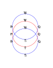
Refer to caption
Refer to caption
Figure 7: Projection curves and approximation curve in Example 1.

We will show several examples to illustrate our algorithm.

Example 1

Consider the algebraic space curve defined by the system {f,g}={x2+y2+z2โˆ’4,(zโˆ’1)โ€‹(x2+y2โˆ’3โ€‹z2)}๐‘“๐‘”superscript๐‘ฅ2superscript๐‘ฆ2superscript๐‘ง24๐‘ง1superscript๐‘ฅ2superscript๐‘ฆ23superscript๐‘ง2\{f,g\}=\{x^{2}+y^{2}+z^{2}-4,(z-1)\,(x^{2}+y^{2}-3\,z^{2})\}. In fact, they are two plane circles with z=ยฑ1๐‘งplus-or-minus1z=\pm 1 as shown in Figure 7 (green ones). The space curve is not irreducible, not regular, and not in a generic position. We will approximate it with rational curves under precision 10โˆ’2superscript10210^{-2}. Following Algorithm 7, we have

  1. 1.

    Compute the resultant of f,g๐‘“๐‘”f,g w.r.t. z๐‘งz, we have ๐’ž1:h=x2+y2โˆ’3=0:subscript๐’ž1โ„Žsuperscript๐‘ฅ2superscript๐‘ฆ230{\mathcal{C}}_{1}:h=x^{2}+y^{2}-3=0, as the red circle in Figure 7. We split ๐’ž1subscript๐’ž1{\mathcal{C}}_{1} into eight regular curve segments with x๐‘ฅx-coordinates [โˆ’1.732050808,โˆ’1.0,0,1.0,1.732050808]1.7320508081.001.01.732050808[-1.732050808,-1.0,0,1.0,1.732050808]: And the tangent directions of the points all are (1,โˆ’โˆ‚hโˆ‚x/โˆ‚hโˆ‚y)1โ„Ž๐‘ฅโ„Ž๐‘ฆ(1,-\frac{\partial h}{\partial x}/\frac{\partial h}{\partial y}) evaluated at these points. Note that x=0๐‘ฅ0x=0 corresponds x๐‘ฅx-critical points of ๐’ž1subscript๐’ž1{\mathcal{C}}_{1} and (ยฑ1.732050808,0)plus-or-minus1.7320508080(\pm 1.732050808,0) correspond to VT points.

  2. 2.

    Since ฯ€yโ€‹(h)=x2โˆ’3subscript๐œ‹๐‘ฆโ„Žsuperscript๐‘ฅ23\pi_{y}(h)=x^{2}-3, we can obtain
    ฮฑ0=โˆ’2,ฮฑ1=โˆ’1.732050808,ฮฑ2=0,ฮฑ3=1.732050808formulae-sequencesubscript๐›ผ02formulae-sequencesubscript๐›ผ11.732050808formulae-sequencesubscript๐›ผ20subscript๐›ผ31.732050808\alpha_{0}=-2,\alpha_{1}=-1.732050808,\alpha_{2}=0,\alpha_{3}=1.732050808, ฮฑ4=2subscript๐›ผ42\alpha_{4}=2. And we can get r=3.464101616๐‘Ÿ3.464101616r=3.464101616. Following Theorem 4, we have R=1.0๐‘…1.0R=1.0 when we choose g๐‘”g to compute R๐‘…R. We can select s=1<r2โ€‹R=1.732050808๐‘ 1๐‘Ÿ2๐‘…1.732050808s=1<\frac{r}{2R}=1.732050808.

  3. 3.

    Compute the resultant of ฯ†โ€‹(f)=fโ€‹(x,y+z,z),ฯ†โ€‹(g)=gโ€‹(x,y+z,z)formulae-sequence๐œ‘๐‘“๐‘“๐‘ฅ๐‘ฆ๐‘ง๐‘ง๐œ‘๐‘”๐‘”๐‘ฅ๐‘ฆ๐‘ง๐‘ง\varphi(f)=f(x,y+z,z),\varphi(g)=g(x,y+z,z) w.r.t. z๐‘งz, we have ๐’ž2:hยฏ=(x2+y2โˆ’2+2โ€‹y)โ€‹(โˆ’2+x2โˆ’2โ€‹y+y2)=0:subscript๐’ž2ยฏโ„Žsuperscript๐‘ฅ2superscript๐‘ฆ222๐‘ฆ2superscript๐‘ฅ22๐‘ฆsuperscript๐‘ฆ20{\mathcal{C}}_{2}:\bar{h}=(x^{2}+y^{2}-2+2\,y)\,(-2+x^{2}-2\,y+y^{2})=0, as two blue circles in Figure 7. Since ฯ€yโ€‹(hยฏ)=(x2โˆ’3)โ€‹(x2โˆ’2)=0subscript๐œ‹๐‘ฆยฏโ„Žsuperscript๐‘ฅ23superscript๐‘ฅ220\pi_{y}(\bar{h})=(x^{2}-3)\,(x^{2}-2)=0, we split ๐’ž2subscript๐’ž2{\mathcal{C}}_{2} into 16 regular curve segments at
    x={โˆ’1.732050808,โˆ’1.414213562,0x=\{-1.732050808,-1.414213562,0, 1.414213562,1.732050808}1.414213562,1.732050808\}. And the tangent directions at the endpoints of these regular curve segments are (1,โˆ‚hยฏโˆ‚x/โˆ‚hยฏโˆ‚y)1ยฏโ„Ž๐‘ฅยฏโ„Ž๐‘ฆ(1,\frac{\partial\bar{h}}{\partial x}/\frac{\partial\bar{h}}{\partial y}) evaluated at the points close to these points. We can get the approximating tangent directions. And we can find that (ยฑ1.732050808,ยฑ1)plus-or-minus1.732050808plus-or-minus1(\pm 1.732050808,\pm 1) are VT points since the absolute values of โˆ‚hยฏโˆ‚x/โˆ‚hยฏโˆ‚yยฏโ„Ž๐‘ฅยฏโ„Ž๐‘ฆ\frac{\partial\bar{h}}{\partial x}/\frac{\partial\bar{h}}{\partial y} evaluated at (ยฑ1.73204,ยฑ1.006118660),(ยฑ1.73204,ยฑ.9938813400)plus-or-minus1.73204plus-or-minus1.006118660plus-or-minus1.73204plus-or-minus.9938813400(\pm 1.73204,\pm 1.006118660),(\pm 1.73204,\pm.9938813400) are larger than 200.

  4. 4.

    As shown in Figure 7, the critical points of ๐’ž1subscript๐’ž1{\mathcal{C}}_{1} are P,Q๐‘ƒ๐‘„P,Q. Choose a vertical line which intersect ๐’ž1subscript๐’ž1{\mathcal{C}}_{1} at W,T๐‘Š๐‘‡W,T. Kโ€‹(K=P,Q,W,T)๐พ๐พ๐‘ƒ๐‘„๐‘Š๐‘‡K(K=P,Q,W,T) are points on ๐’ž1subscript๐’ž1{\mathcal{C}}_{1} and K1,K2subscript๐พ1subscript๐พ2K_{1},K_{2} are corresponding points of K๐พK on ๐’ž2subscript๐’ž2{\mathcal{C}}_{2}. Consider Wโ€‹(0,1.732050808),W1โ€‹(0,2.732050808),W2โ€‹(0,0.732050808)๐‘Š01.732050808subscript๐‘Š102.732050808subscript๐‘Š200.732050808W(0,1.732050808),W_{1}(0,2.732050808),W_{2}(0,0.732050808) for example. We can find that W1,W2subscript๐‘Š1subscript๐‘Š2W_{1},W_{2} are on the line x=0๐‘ฅ0x=0 in a neighborhood with radius 1.7320508081.7320508081.732050808 centered at W๐‘ŠW. So we can conclude that W1,W2subscript๐‘Š1subscript๐‘Š2W_{1},W_{2} correspond to W๐‘ŠW with local generic position method. The correspondence of other points are similar.

  5. 5.

    Approximate ๐’ž1,๐’ž2subscript๐’ž1subscript๐’ž2{\mathcal{C}}_{1},{\mathcal{C}}_{2} respectively. In order to derive the required precision 10โˆ’2superscript10210^{-2}, we we use precision ฯต1=0.0044<112+4โ€‹10โˆ’2subscriptitalic-ฯต10.00441superscript124superscript102\epsilon_{1}=0.0044<\frac{1}{\sqrt{1^{2}+4}}10^{-2} for the regular curve segments of ๐’ž1,๐’ž2subscript๐’ž1subscript๐’ž2{\mathcal{C}}_{1},{\mathcal{C}}_{2} without VT point(s), and we use precision ฯต2=0.0022<12โ€‹12+4โ€‹10โˆ’2subscriptitalic-ฯต20.002212superscript124superscript102\epsilon_{2}=0.0022<\frac{1}{2\sqrt{1^{2}+4}}10^{-2} for the regular curve segments with VT point. Consider a regular curve segments on ๐’ž1subscript๐’ž1{\mathcal{C}}_{1}, (โˆ’1.732050808,0),(โˆ’1.60,0.6633249580)1.73205080801.600.6633249580(-1.732050808,0),(-1.60,0.6633249580) are the endpoints for the one, denoted as C1subscript๐ถ1C_{1}. And it has a VT point. (โˆ’1.60,0.6633249580),(โˆ’1.40,1.019803903)1.600.66332495801.401.019803903(-1.60,0.6633249580),(-1.40,1.019803903) are endpoints for the other, denoted as C2subscript๐ถ2C_{2}. And it has no VT point. The approximation of C1subscript๐ถ1C_{1} is (x,0.9999999059โ€‹โˆ’x2+0.000000464โ€‹x+3.000000806),xโˆˆ[โˆ’1.732050808,โˆ’1.60]๐‘ฅ0.9999999059superscript๐‘ฅ20.000000464๐‘ฅ3.000000806๐‘ฅ1.7320508081.60(x,0.9999999059\,\sqrt{-x^{2}+0.000000464\,x+3.000000806}),x\in[-1.732050808,-1.60] and the error is very small. The approximation for C2subscript๐ถ2C_{2} is (x,0.6106757885x+2.310809554โˆ’0.1270414345/(0.5070598449x+1.0),xโˆˆ[โˆ’1.60,โˆ’1.40](x,0.6106757885\,x+2.310809554-0.1270414345/(0.5070598449\,x+1.0),x\in[-1.60,-1.40] and the error is 0.0004<ฯต10.0004subscriptitalic-ฯต10.0004<\epsilon_{1}. For the regular curve segments on ๐’ž2subscript๐’ž2{\mathcal{C}}_{2} with endpoints: [(โˆ’1.732050808,1.0)[(-1.732050808,1.0), (โˆ’1.60,1.663324958)](-1.60,1.663324958)], denoted as C3subscript๐ถ3C_{3} and it has a VT point. (โˆ’1.60(-1.60, 1.663324958)1.663324958), (โˆ’1.414213562,2.0)1.4142135622.0(-1.414213562,2.0) are endpoints for the other, denoted as C4subscript๐ถ4C_{4}, without VT point. Similarly as C1subscript๐ถ1C_{1}, the approximation for C3subscript๐ถ3C_{3} is (x,1.0+0.9999999054โˆ’x2+0.000000466โ€‹x+3.000000809,xโˆˆ[โˆ’1.732050808,โˆ’1.60].(x,1.0+0.9999999054\,\sqrt{-x^{2}+0.000000466\,x+3.000000809},x\in[-1.732050808,-1.60]. The approximation for C4subscript๐ถ4C_{4} is (x,0.6301674345โ€‹x+3.324059999โˆ’0.1265242054/(0.5086364591โ€‹x+1.0)),xโˆˆ[โˆ’1.60,โˆ’1.414213562]๐‘ฅ0.6301674345๐‘ฅ3.3240599990.12652420540.5086364591๐‘ฅ1.0๐‘ฅ1.601.414213562(x,0.6301674345\,x+3.324059999-0.1265242054/(0.5086364591\,x+1.0)),x\in[-1.60,-1.414213562] and the error is 0.0002<ฯต10.0002subscriptitalic-ฯต10.0002<\epsilon_{1}. We can find that parts of C1,C2subscript๐ถ1subscript๐ถ2C_{1},C_{2} and C3,C4subscript๐ถ3subscript๐ถ4C_{3},C_{4} are correspondent.

  6. 6.

    Recover the approximation space curves of fโˆงg๐‘“๐‘”f\wedge g by the formula z=y2โ€‹(x)โˆ’y1โ€‹(x)s๐‘งsubscript๐‘ฆ2๐‘ฅsubscript๐‘ฆ1๐‘ฅ๐‘ z=\frac{y_{2}(x)-y_{1}(x)}{s}. The space regular curve segment corresponding to C1subscript๐ถ1C_{1} and C3subscript๐ถ3C_{3}, we have its approximation parametric space regular curve segment for xโˆˆ[โˆ’1.732050808,โˆ’1.60]๐‘ฅ1.7320508081.60x\in[-1.732050808,-1.60]:

    (x,0.9999999059โˆ’x2+0.000000464โ€‹x+3.000000806,\displaystyle(x,0.9999999059\,\sqrt{-x^{2}+0.000000464\,x+3.000000806},
    1.0+0.9999999054โ€‹โˆ’x2+0.000000466โ€‹x+3.0000008091.00.9999999054superscript๐‘ฅ20.000000466๐‘ฅ3.000000809\displaystyle 1.0+0.9999999054\,\sqrt{-x^{2}+0.000000466\,x+3.000000809}
    โˆ’0.9999999059โˆ’x2+0.000000464โ€‹x+3.000000806).\displaystyle-0.9999999059\,\sqrt{-x^{2}+0.000000464\,x+3.000000806}).

    The approximation space curve is not rational, denoted as S1subscript๐‘†1S_{1}. The approximation corresponding to C2,C4subscript๐ถ2subscript๐ถ4C_{2},C_{4} for xโˆˆ[โˆ’1.60,โˆ’1.414213562]๐‘ฅ1.601.414213562x\in[-1.60,-1.414213562], denoted as S2subscript๐‘†2S_{2}, is
    (x,0.6106757885x+2.310809554โˆ’0.12704143450.5070598449โ€‹x+1.0,(x,0.6106757885\,x+2.310809554-\frac{0.1270414345}{0.5070598449\,x+1.0},
    0.0194916460x+1.013250445โˆ’0.12652420540.5086364591โ€‹x+1.0+0.12704143450.5070598449โ€‹x+1.0).0.0194916460\,x+1.013250445-\frac{0.1265242054}{0.5086364591\,x+1.0}+\frac{0.1270414345}{0.5070598449\,x+1.0}).

  7. 7.

    We will re-parameterize S1subscript๐‘†1S_{1} into rational one. At first, we can find that the y๐‘ฆy coordinate of S1subscript๐‘†1S_{1} changes from 00 to 0.66332495800.66332495800.6633249580. Its two endpoints are P0โ€‹(โˆ’1.732050808,0,1.0),P1โ€‹(โˆ’1.60,0.6633249580,1.0)subscript๐‘ƒ01.73205080801.0subscript๐‘ƒ11.600.66332495801.0P_{0}(-1.732050808,0,1.0),P_{1}(-1.60,0.6633249580,1.0). The tangent direction of S2subscript๐‘†2S_{2} at P2subscript๐‘ƒ2P_{2} is (1,2.412090757,0.0)12.4120907570.0(1,2.412090757,0.0). By approximating the tangent direction of S1subscript๐‘†1S_{1} at P1subscript๐‘ƒ1P_{1}, we have (1,283.0783218,0.0)1283.07832180.0(1,283.0783218,0.0). And there is another regular curve segment which shares a same tangent direction with S1subscript๐‘†1S_{1} at P1subscript๐‘ƒ1P_{1}. Taking their average value, we can set the tangent direction of S1subscript๐‘†1S_{1} at P1subscript๐‘ƒ1P_{1} as (0,1,0)010(0,1,0). Using Formula (11), we can easily obtain the rational approximation regular curve segment for S1subscript๐‘†1S_{1} is
    (โˆ’2.412090984โ€‹yโˆ’22.71853197+20.98648116โˆ’0.1149354656โ€‹y+1,y,1.0).2.412090984๐‘ฆ22.7185319720.986481160.1149354656๐‘ฆ1๐‘ฆ1.0(-2.412090984\,y-22.71853197+\frac{20.98648116}{-0.1149354656\,y+1},y,1.0).
    The error in x๐‘ฅx-direction is 0.0020563160<ฯต20.0020563160subscriptitalic-ฯต20.0020563160<\epsilon_{2}, (We take 19 sample points besides endpoints to compute the error.). So the approximation rational curve satisfies the error requirement.

  8. 8.

    Output the piecewise approximation curve.

Example 2

Approximate the algebraic space curve defined by f=g=0๐‘“๐‘”0f=g=0, where f=x2+y2+z2โˆ’4,g=(x2+y2+2โ€‹yโˆ’z2)โ€‹(zโˆ’xโˆ’4โ€‹y)formulae-sequence๐‘“superscript๐‘ฅ2superscript๐‘ฆ2superscript๐‘ง24๐‘”superscript๐‘ฅ2superscript๐‘ฆ22๐‘ฆsuperscript๐‘ง2๐‘ง๐‘ฅ4๐‘ฆf={x}^{2}+{y}^{2}+{z}^{2}-4,g=\left({x}^{2}+{y}^{2}+2\,y-{z}^{2}\right)\left(z-x-4\,y\right). It is a space curve with singular point. The approximation space curve is as the left part of Figure 8 and the error is 0.013. The color differs the different approximating space regular curve segments.
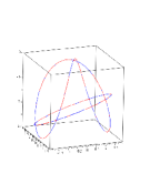
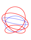
Refer to caption
Refer to caption
Figure 8: Appriximation curve and projection curves in Example 2.
Example 3

In this example, we will approximate the algebraic space curve defined by f=g=0๐‘“๐‘”0f=g=0 inside [โˆ’2,2]ร—[โˆ’2,2]ร—[โˆ’2,2]222222[-2,2]\times[-2,2]\times[-2,2] with error ฯต=0.014italic-ฯต0.014\epsilon=0.014, where f=95โˆ’94โ€‹x3+64โ€‹x2โ€‹y+28โ€‹x2โ€‹zโˆ’61โ€‹x2+69โ€‹xโ€‹y2โˆ’53โ€‹xโ€‹yโ€‹zโˆ’59โ€‹xโ€‹y+28โ€‹xโ€‹z2โˆ’15โ€‹xโ€‹zโˆ’83โ€‹xโˆ’3โ€‹y3+59โ€‹y2โ€‹z+49โ€‹y2+4โ€‹yโ€‹z2+11โ€‹yโ€‹z+5โ€‹yโˆ’81โ€‹z3โˆ’8โ€‹z2โˆ’9โ€‹z,g=49+7โ€‹x3โˆ’46โ€‹x2โ€‹y+87โ€‹x2โ€‹z+94โ€‹x2+73โ€‹xโ€‹y2+93โ€‹xโ€‹yโ€‹zโˆ’3โ€‹xโ€‹yโˆ’27โ€‹xโ€‹z2+56โ€‹xโ€‹z+70โ€‹x+72โ€‹y3โˆ’37โ€‹y2โ€‹zโˆ’20โ€‹y2+79โ€‹yโ€‹z2โˆ’78โ€‹yโ€‹zโˆ’3โ€‹y+94โ€‹z3+30โ€‹z2+47โ€‹zformulae-sequence๐‘“9594superscript๐‘ฅ364superscript๐‘ฅ2๐‘ฆ28superscript๐‘ฅ2๐‘ง61superscript๐‘ฅ269๐‘ฅsuperscript๐‘ฆ253๐‘ฅ๐‘ฆ๐‘ง59๐‘ฅ๐‘ฆ28๐‘ฅsuperscript๐‘ง215๐‘ฅ๐‘ง83๐‘ฅ3superscript๐‘ฆ359superscript๐‘ฆ2๐‘ง49superscript๐‘ฆ24๐‘ฆsuperscript๐‘ง211๐‘ฆ๐‘ง5๐‘ฆ81superscript๐‘ง38superscript๐‘ง29๐‘ง๐‘”497superscript๐‘ฅ346superscript๐‘ฅ2๐‘ฆ87superscript๐‘ฅ2๐‘ง94superscript๐‘ฅ273๐‘ฅsuperscript๐‘ฆ293๐‘ฅ๐‘ฆ๐‘ง3๐‘ฅ๐‘ฆ27๐‘ฅsuperscript๐‘ง256๐‘ฅ๐‘ง70๐‘ฅ72superscript๐‘ฆ337superscript๐‘ฆ2๐‘ง20superscript๐‘ฆ279๐‘ฆsuperscript๐‘ง278๐‘ฆ๐‘ง3๐‘ฆ94superscript๐‘ง330superscript๐‘ง247๐‘งf=95-94\,{x}^{3}+64\,{x}^{2}y+28\,{x}^{2}z-61\,{x}^{2}+69\,x{y}^{2}-53\,xyz-59\,xy+28\,x{z}^{2}-15\,xz-83\,x-3\,{y}^{3}+59\,{y}^{2}z+49\,{y}^{2}+4\,y{z}^{2}+11\,yz+5\,y-81\,{z}^{3}-8\,{z}^{2}-9\,z,g=49+7\,{x}^{3}-46\,{x}^{2}y+87\,{x}^{2}z+94\,{x}^{2}+73\,x{y}^{2}+93\,xyz-3\,xy-27\,x{z}^{2}+56\,xz+70\,x+72\,{y}^{3}-37\,{y}^{2}z-20\,{y}^{2}+79\,y{z}^{2}-78\,yz-3\,y+94\,{z}^{3}+30\,{z}^{2}+47\,z. The approximation space curve is as Figure 9.
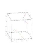
Refer to caption
Refer to caption
Figure 9: Appriximation curve and projection curves in Example 3.

5 Conclusion

We introduce a local generic position method to compute the topology as well as the piecewise approximation curves of algebraic space curves. Especially, we present an algorithm to approximate algebraic space curve by piecewise rational curves with correct topology and under any given precision. The method is effective.

Acknowledgement

The work is partially supported by NKBRPC (2011CB302400), NSFC Grants (60821002, 11001258, 91118001), and China-France cooperation project EXACTA (60911130369).

References and Notes

  • [1] S.S. Abhyankar and C. Bajaj. Automatic parameterization of rational curves and surfaces IV: algebraic space curves. ACM Trans. Graph., 8:325โ€“334, October 1989.
  • [2] L. Alberti, B. Mourrain, J. Wintz. Topology and arrangement computation of semi-algebraic planar curves. Computer Aided Geometric Design, 25(8): 631โ€“651, 2008.
  • [3] J.G. Alcazยดยด๐‘ง\acute{z}ar, and J.R Sendra. Computation of the topology of algebraic space curves. Journal of Symbolic Computation, Vol. 39, No. 6, 719โ€“744, 2005.
  • [4] D. Arnon, S. McCallum. A polynomial time algorithm for the topological type of a real algebraic curve. Journal of Symbolic Computation 5: 213โ€“236, 1988.
  • [5] C. L. Bajaj, C. Hoffmann, J. Hopcroft, R. Lynch. Tracing surface intersections. Computer Aided Geometric Design 5(4): 285โ€“307, 1988.
  • [6] C. L. Bajaj and G. Xu, NURBS approximation of surface/surface intersection curves, Advances in Computational Mathematics, Volume 2, Number 1, 1โ€“21, 1994.
  • [7] S. Beยดยด๐‘’\acute{e}la B. Juยจยจ๐‘ข\ddot{u}ttler, Approximating Algebraic Space Curves by Circular Arcs, DK-Report No. 2010.12. A C4040 LINZ, 2010.
  • [8] E. Berberich, P. Emeliyanenko, A. Kobel and M. Sagraloff. Exact Symbolic-Numeric Computation of Planar Algebraic Curves, online, 2012.
  • [9] T.G. Berry, Parameterization of algebraic space curves, Journal of Pure and Applied Algebra Volumes 117โ€“118, May 1997, Pages 81โ€“95.
  • [10] M. Bizzarri and M. Laยดยด๐‘Ž\acute{a}viห‡ห‡๐‘–\check{i}cka. Algorithm for parameterization of rational curves revisited. Journal for Geometry and Graphics, 15(1):1โ€“18, 2011.
  • [11] M. Burr, S. W. Choi, B. Galehouse, C.-K. Yap, Complete subdivision algorithms, II: isotopic meshing of singular algebraic curves. ISSAC 2008: 87โ€“94.
  • [12] J. S. Cheng, X. S. Gao, J. Li. Root isolation for bivariate polynomial systems with local generic position method. ISSAC 2009: 103โ€“110, 2009.
  • [13] J. S. Cheng, X. S. Gao, L. Guo. Root Isolation of Zero-dimensional Polynomial Systems with Linear Univariate Representation. Accepted by J. Symb. Comp. also in CoRR abs/1102.4681: (2011).
  • [14] J. S. Cheng, S. Lazard, L. Pen~~๐‘›\tilde{n}aranda, M. Pouget, F. Rouillier and E. Tsigaridas, On the topology of real algebraic plane curves, Mathematics in Computer Science, Volume 4, Number 1, 113-137, 2010.
  • [15] J. Chuang, C. Hoffmann. On local implicit approximation and its application. ACM Trans. Graph. 8 (4), 298โ€“324, 1989.
  • [16] D. N. Daouda, B. Mourrain, O. Ruatta. On the computation of the topology of a non-reduced implicit space curve. ISSAC 2008, 47โ€“54, 2008.
  • [17] L. Dupont, D. Lazard, S. Lazard, S. Petitjean. Near-Optimal Parameterization of the Intersection of Quadrics: I. The Generic Algorithm. Journal of Symbolic Computation, 43 (3): 168โ€“191, 2008.
  • [18] L. Dupont, D. Lazard, S. Lazard, S. Petitjean. Near-Optimal Parameterization of the Intersection of Quadrics: II. A Classification of Pencils. Journal of Symbolic Computation, 43 (3): 192โ€“215, 2008.
  • [19] L. Dupont, D. Lazard, S. Lazard, S. Petitjean. Near-Optimal Parameterization of the Intersection of Quadrics: III. Parameterizing Singular Intersections. Journal of Symbolic Computation, 43 (3): 216โ€“232, 2008.
  • [20] A. Eigenwilling, M. Kerber. Exact and efficient 2d-arrangements of arbitrary algebraic curves. In: Proc. 19th Annual ACM-SIAM Symposium on Discrete Algorithms (SODA08), San Francisco, USA, January 2008, pp. 122โ€“131. ACM-SIAM, ACM/SIAM, 2008.
  • [21] J. Gahleitner, B. Juยจยจ๐‘ข\ddot{u}ttler, J. Schicho. Approximate Parameterization of Planar Cubic curve segments. Proc. Fifth International Conference on Curves and Surfaces. Saint-Malo 2002. pp. 1โ€“13, Nashboro Press, Nashville, TN.
  • [22] X.-S. Gao, S.C. Chou. On the parameterization of algebraic curves. Applicable Algebra in Elementary Communication and Computing 3: 27โ€“38, 1992.
  • [23] X.-S. Gao, M. Li. Rational quadratic approximation to real algebraic curves, Computer Aided Geometric Design 21: 805โ€“828, 2004.
  • [24] G. Gatellier, A. Labrouzy, B. Mourrain, and J.P. T ecourt. Computing the topology of three-dimensional algebraic curves. Computational methods for algebraic spline surfaces, 27โ€“43, Springer, Berlin, 2005.
  • [25] L. Gonzalez-Vega, I. Necula. Efficient topology determination of implicitly defined algebraic plane curves. Computer Aided Geometry Design, vol. 19, no. 9, 719โ€“743, 2002.
  • [26] E. Hartmann, (2000). Numerical Parameterization of Curves and Surfaces. Computer Aided Geometry Design, Vol. 17. pp. 251-266.
  • [27] M. van Hoeij. Rational parametrizations of algebraic curves using a canonical divisor. Journal of Symbolic Computation, 23:209โ€“227, 1997.
  • [28] H. Hong. An efficient method for analyzing the topology of plane real algebraic curves. Math. and Comp. Sim. 42 (1996) 541โ€“582.
  • [29] B. Juยจยจ๐‘ข\ddot{u}ttler and P. Chalmovianskyยดยด๐‘ฆ\acute{y}. A predictor-corrector-type technique for the approximate parameterization of intersection curves. Applicable Algebra in Engineering, Communication and Computing, 18: 151โ€“168, January 2007.
  • [30] M. El Kahoui. Topology of real algebraic space curves. Journal of Symbolic Computation. Volume 43 Issue 4, April, 2008.
  • [31] S. Krishnan, D.Manocha. An efficient surface intersection algorithm based on lower-dimensional formulation. ACM Trans. Graph. 16(1): 74โ€“106, 1997.
  • [32] C. Liang, B. Mourrain, J.-P. Pavone. Subdivision Methods for the Topology of 2d and 3d Implicit Curves, In piene, R., Juยจยจ๐‘ข\ddot{u}ttler, B. eds.: Geometric Modeling and Algebraic Geometry. Springer, 199โ€“214, 2008.
  • [33] J.C. Owen, A.P. Rockwood. Intersection of general implicit surfaces. In Geometric modeling, SIAM, 335โ€“345, 1987.
  • [34] N.M. Patrikalakis. Surface-to-Surface Intersections. IEEE Comput. Graph. Appl. 13(1): 89โ€“95, 1993.
  • [35] S. Peยดยด๐‘’\acute{e}rez-Diยดยด๐‘–\acute{i}az, S.L. Rueda, J. Sendra, J.R. Sendra. Approximate Parametrization of Plane Algebraic Curves by Linear Systems of Curves. Computer Aided Geometric Design, vol 27, 212โ€“231, 2010.
  • [36] M.J. Pratt, A.D. Geisow. Surface/surface intersection problem. In Gregory, J., ed.: The Mathematics of Surfaces II. Claredon Press, Oxford, 117โ€“142, 1986.
  • [37] S. L. Rueda, J. Sendra, J. R. Sendra. Approximate parametrization of space algebraic curves. online 2012.
  • [38] T. Sakkalis. The topological configuration of a real algebraic curve. Bull. Aust. Math. Soc. 43: 37โ€“50, 1991.
  • [39] J. Schicho. On the choice of pencils in the parametrization of curves. Journal of Symbolic Computation, 14:557โ€“576, December 1992.
  • [40] R. Seidel, N. Wolpert. On the exact computation of the topology of real algebraic curves. In: Proc 21st ACM Symposium on Computational Geometry, pp. 107โ€“115, 2005.
  • [41] J. R. Sendra, F. Winkler. Symbolic parametrization of curves. Journal of Symbolic Computation, 12(6):607โ€“631, 1991.
  • [42] L.Y. Shen, C.M. Yuan, X.S. Gao. Certified Approximation of Parametric Space Curves with Cubic B-spline Curves. Preprint 2011.
  • [43] C.H. Tu, W. Wang, B. Mourrain, J.Y. Wang. Using signature sequences to classify intersection curves of two quadrics. Computer Aided Geometric Design, 26: 317โ€“335, 2009.
  • [44] R. Walker. Algebraic Curves. Springer-Verlag, New York, 1978.
  • [45] W. Wang, R. Goldman, C.H. Tu. Enhancing Levinโ€™s method for computing quadric surface intersections. Computer Aided Geometric Design, 20: 401โ€“ 422, 2003.