A discrete estimation of the uncertainty of the background redshift and its effects on cosmological parameters

Abstract

We develop a discrete model to account for the effects of inhomogeneities on the redshift of photons. Using this model we compute the probability distribution of the observed redshift respect to the background value, obtaining that its dispersion around the central value is proportional the square root of the comoving distance. This implies that data analysis should include a contribution to the total error budget which depends on the distance of the source. Assuming large scale inhomogeneities with a power spectrum given by primordial curvature perturbations the effect is expected to be small at low red-shift, and to become important only at very high redshift. We then consider what are the general implications for the estimation of background cosmological parameters, giving some example for the case of quantities related to the luminosity distance such as the Hubble parameter and the cosmological constant.

The model correctly reproduces the expected stochastic properties of the propagation of photons in inhomogeneous media and due to its computational simplicity it could be particularly suitable for the numerical estimation of the effects of inhomogeneities on cosmological observables using Montecarlo methods.

I Introduction

Cosmology has some distinctive features respect to other branches of physics: we can observe the Universe only from one point, and we are unable to probe directly the geometry of space-time on large scales. We can only detect particles or radiation which have reached us, and extract from these observations information about the space-time between us and the sources. Most of cosmological scale distances can in fact only be deduced from redshift measurements, assuming an underlying space-time metric. The Hubble law for example is based on the assumption of large scale isotropy and homogeneity of the metric describing the Universe. We know nevertheless that the Universe had inhomogeneities since very early times, as predicted by inflation, which are supposed to be the seeds for the later process of structure formation due to gravity. There has been an long debate us ; buchert ; nambu ; wald ; tomita on whether these perturbations of the homogeneous space-time metric could explain cosmological observations, in particular if they could induce effects equivalent to a cosmological constant or dark energy. In this paper we consider what are the statistical effects of these inhomogeneities on the determination of background cosmological parameters, focusing on their complementary role rather than looking at them as alternatives dark energy for example. It was shown in fact that even in presence of dark energy inhomogeneities could play an important role in affecting the determination of the background cosmological parameters Romano:2015iwa ; Romano:2011mx ; Romano:2014iea ; EneaRomano:2011aa

The paper is organized as follows. We fist develop a discrete model of the inhomogeneities through which photons propagate from the source to the observer. We then use this model to estimate the effects of inhomogeneities on the determination of cosmological parameters and obtain the distribution probability function (PDF) for the redshift correction, showing that its dispersion around the central value is proportional to the square root of the comoving distance. We then study the general implications on the estimation of background cosmological observables considering in particular the case of quantities related to the luminosity distance such as the Hubble parameter and the cosmological constant.

II Effects of inhomogeneities on the luminosity distance

Let’s consider a Friedman universe with scalar perturbations. In longitudinal gauge the metric can be written as

$$ds^{2}=-(1+2\Psi)d\eta^{2}+(1-2\Psi)\delta_{ij}dx^{i}dx^{j}~{}.$$ (1)

where we have assumed assumed for simplicity the background to be flat and the perturbations to be of perfect fluid type. Lets us suppose Sasaki ; Dyer ; Bonvin:2005ps a photon is emitted from a source located at a comoving coordinate $r_{S}$ and time $t_{S}$ with a wave length $\lambda_{S}$, and is reaching an observer at the center $r_{O}=0$, with a wavelength $\lambda_{O}$ . Its total redshift can be expressed as the sum of two components . One is due to the homogeneous background expansion, $z_{H}$, and another due to the perturbations of the gravitation potential, $z_{I}$ :

$$\frac{\lambda_{O}}{\lambda_{S}} = 1+z=1+z_{H}+z_{I}+z_{OS}=\frac{a(t_{O})}{a(t_{S})}(1+\left[\psi+{\mathbf{v}}\cdot{\mathbf{n}}\right]^{O}_{S}-2\int_{\lambda_{S}}^{\lambda_{O}}d\lambda\dot{\psi}~{})~{},$$ (2)

$$z_{H} = \frac{a(t_{O})}{a(t_{S})}-1~{},$$ (3)

$$z_{I} = (1+z_{H})(-2\int_{\lambda_{S}}^{\lambda_{O}}d\lambda\dot{\psi}~{})~{},$$ (4)

$$z_{OS} = (1+z_{H})(\left[\psi+{\mathbf{v}}\cdot{\mathbf{n}}\right]^{O}_{S}~{})~{}$$ (5)

where we are denoting with a dot the derivative respect to conformal time $\eta$.

III Discrete approach

In the following we will focus on the contribution $z_{I}$ coming from the integral, since we are interested in the cumulative effects of the structure between the source and observer. The other term $z_{OS}$ associated to the difference of the peculiar velocity and gravitational potential between the source and the observer is also important, but accurate observations of the source and information about our local Universe allow to determine it directly, making it a not major source of uncertainty on the observed redshift, with most of the uncertainty coming from the propagation of the errors of observationally estimated $\psi$ and $v$ of the source and the observer. See for example Riess:2016jrr and references therein for an example of how density maps can be used to reconstruct the peculiar velocity and gravitational potential fields of the source using cosmological perturbation theory. For a non linear treatment see Vallejo:2017rga .

On the contrary the term $z_{I}$ associated to the integral is not under direct observational control because for a given source we do not exactly know what is the structure between it and the observer, and the effects on the photons propagating through it are expected to increase with the distance.

We can approximate $z_{I}$ discretely with

$$z_{I} = (1+z_{H})(-2\int_{\lambda_{S}}^{\lambda_{O}}d\lambda\dot{\psi}~{})\approx-2(1+z_{H})\Delta r\sum_{i=1}^{N}\dot{\psi}~{},$$ (6)

where in the last approximate equality we have chosen the comoving coordinate as the affine parameter along the null geodesic, we have divided the interval $(r_{S},0)$ into N subintervals of equal comoving length $\Delta r$ and approximated the integral with a sum.

Figure 1: The probability distribution for $P(z_{I}/\Delta z_{min})$ is plotted for different values of N. The thick line is for $N=30$, the dash-dotted line is for $N=20$, and the dashed line is for $N=10$. The difference between the different distributions is due to the fact that as N increases $\Delta r$ decreases, lowering $\Delta z_{min}$. As it can be seen the dispersion increases with N.

The time evolution of the Fourier transform of the gravitational potential is given by:

$$\dot{\psi_{k}} = \psi_{P}(k)T(k)\frac{d}{d\eta}\bigg{(}\frac{D(\eta)}{a(\eta)}\bigg{)}~{},$$ (7)

where $D(\eta)$ is the growth factor, $T(k)$ is the transfer function, and $\psi_{P}(k)$ is the primordial perturbation. For a matter dominated universe the time derivative of the gravitational potential is zero, while for a Universe with cosmological constant there can be a significant contribution, which in the case of the cosmic microwave background radiation for example leads to the so called integrated ISW effect.

We can approximate the Gaussian distribution with a uniform discrete distribution for a variable $X$ with three possible values

$$\{x_{1},x_{2},x_{3}\}=\{\sigma_{\psi},0,-\sigma_{\psi}\}.$$ (8)

After substituting we get

$$z_{I} = -2(1+z_{H})\Delta r\sum_{i=1}^{N}\alpha_{i}\psi_{i}~{},$$ (9)

where $\alpha_{i}$ is the value in the $i-th$ sub-interval of $\frac{d}{d\eta}\bigg{(}\frac{D(\eta)}{a(\eta)}\bigg{)}$ and $\psi_{i}$ is the value of the discrete random variable $X$ in the $i-th$ sub-interval determined by the time independent part of the $\psi(k,\eta)$, i.e. by $\psi_{P}(k)T(k)$. For large scales $T(k)$ is approximately 1, so $\psi_{i}$ is of the order of the primordial spectrum $\psi_{P}(k)$.

Figure 2: Two configurations of the discrete variable $\psi_{i}$ are shown as a function of the comoving distance. They both correspond to $\{n_{+}=3,n_{-}=1,S=2\}$ and consequently produce the same redshift correction $z_{I}$ as shown in eq.(37). This kind of degeneracy increases with the number of sub-intervals $N$ and implies a larger dispersion around the central value as shown in fig.(48).

IV trinomial discrete approximation of a Gaussian process

Assuming the primordial gravitational potential to be a treee dimesional Gaussian field, as predicted by many inflationary models and supported by cosmic microwave observations, also the gravitational potential along the propagation path will be a one-dimensional Gaussian field, as shown in section VI. We can then approximate it as a sequence of discrete random variables $\psi_{i}$, which can have three possible values: zero and plus or minus the standard deviation of the Gaussian field $\sigma_{\psi}$, with appropriate probabilities. The scaling limit of the sum of these variables is a trinomial discrete approximation of the Brownian motion, as implied by the Donsker’s theorem, also know as functional central limit theorem. In principle also a binomial approximation would suffice to get the right scaling limit as long as the variance and the mean are the same, but the advantage of the trinomial is that it can accommodate time varying variance. This is indeed modeling well the effect we are interesting in, since $\frac{d}{d\eta}\left(\frac{D}{a}\right)$ effectively changes the value of the standard deviation at different points along the path.

We have proposed a discrete model for the propagation of photons in an inhomogeneous medium. The large N limit of this discrete model has to coincide with its continuos equivalent. We are modelling the potential along the photon path as a Gaussian process which can be approximated as a sequence of independent identically distributed random variables. This discrete model is valid for processes with constant power spectrum, i.e. white noise, and since the primordial curvature perturbations are approximately scale invariant, it should indeed be a good approximation.

The effect we are interested is the integral of this Gaussian process, which is known to be a Browninan motion, and in fact our results will confirm this. A Gaussian process with constant spectrum $\sigma^{2}$ can be approximated as a sequence of random Gaussian variables with variance $\sigma^{2}/\Delta r$ sigmawhite , where the interval over which the process is sampled discretely has been divided in $N=r/\Delta r$ sub-intervals. Under this discretization scheme in fact the integral of the Gaussian process is

$$I = \int^{r}_{0}X(r)dr\approx\sum^{N}_{i=1}\Delta rX_{i}$$ (10)

and since the variance of the a linear combination of a set of Gaussian variables $X_{i}$

$$Z=\sum^{N}_{i=1}c_{i}X_{i}$$ (11)

has variance

$$\sigma_{Z}^{2}=\sum^{N}_{i=1}c_{i}^{2}\sigma_{X_{i}}^{2}$$ (12)

from $\sigma_{X_{i}}^{2}=\sigma^{2}/\Delta r$ we get

$$\sigma^{2}_{I}=N\Delta r^{2}\frac{\sigma^{2}}{\Delta r}=N\Delta r\sigma^{2}=r\sigma^{2}$$ (13)

As expected in a Browonian motion, which is the integral of a Gaussian process of the type we considered, the variance is linear in the time variable, which in this case is the conformal time, or equivalently since we are assuming a flat background, the comoving distance.

V Mean and variance of the variable s

Putting all together we can model the integrand $Y_{i}=\alpha_{i}\psi_{i}$ in each interval with a uniformly distributed discrete random variable which can take three values

$$\{Y_{i,1},Y_{i,2},Y_{i,3}\}=\{\frac{\sigma\alpha_{i}}{\sqrt{\Delta r}},0,-\frac{\sigma\alpha_{i}}{\sqrt{\Delta r}}\}$$ (14)

where we are using the notation $Y_{i,j}$ for the j-th value of the i-th variable and we are denoting $\sigma_{\psi}$ with $\sigma$. We can define the single variable MGF for $Y_{i}$ as

$$M_{\tilde{Y_{i}}}(t) = E[e^{tY_{i}}]=\sum p_{j}e^{tY_{i,j}}=\frac{1}{3}\left[1+\exp{\left(\frac{\sigma\alpha_{i}t}{\sqrt{\Delta r}}\right)}+\exp{\left(\frac{-\sigma\alpha_{i}t}{\sqrt{\Delta r}}\right)}\right]\,.$$ (15)

from which we can get the mean and variance

$$\mu_{Y_{i}} = E[Y_{i}]=M_{Y_{i}}^{\prime}(0)=0\,,$$ (16)

$$\sigma^{2}_{Y_{i}} = Var[Y_{i}]=E[Y_{i}^{2}]-E[Y_{i}]^{2}=M_{Y_{i}}^{\prime\prime}(0)=\frac{2}{3}\frac{\sigma^{2}\alpha_{i}^{2}}{\Delta r}\,.$$ (17)

From eq.(9) we can see that the effect we are interested in is proportional to the variable $S$ defined as

$$S = \sum^{N}_{i}\Delta rY_{i}\,$$ (18)

$$z_{I} = -2(1+z_{H})\Delta r\sum_{i=1}^{N}Y_{i}=-2(1+z_{H})\,S~{},$$ (19)

Assuming $Y_{i}$ are mutually independent, i.e. as mentioned previously, modeling the Gaussian process with an approximately constant spectrum, the MGF for $S$ is given by the product of single variable MGF

$$M_{S}(t) = \prod^{N}_{i}M_{Y_{i}}(\Delta r\,t)\,.$$ (20)

We can now compute mean and variance of $S$

$$\mu_{S} = E[S]=M_{S}^{\prime}(0)=0\,,$$ (21)

$$\sigma^{2}_{S} = Var[S]=E[S^{2}]-E[S]^{2}=M_{S}^{\prime\prime}(0)-M_{S}^{\prime}(0)^{2}$$ (22)

$$= \sum^{N}_{i}\Delta r^{2}\sigma_{Y_{i}}^{2}=\frac{2}{3}\sigma^{2}\sum^{N}_{i}\alpha_{i}^{2}\Delta r\,.$$ (23)

In the continuos limit we get

$$\sigma^{2}_{S}(z_{H}) = \frac{2}{3}\sigma^{2}\int^{r(z_{H})}_{0}\alpha(r)^{2}dr=\sigma^{2}\beta(z_{H})\,,$$ (24)

$$\beta(z_{H}) = \frac{2}{3}\int^{r(z_{H})}_{0}\alpha(r)^{2}dr\,.$$ (25)

Defining

$$\overline{\alpha}^{2} = \frac{2}{3N}\sum^{N}_{i}\alpha_{i}^{2}=\frac{2}{3N\Delta r}\sum^{N}_{i}\alpha_{i}^{2}\Delta r\rightarrow\frac{2}{3r(z_{H})}\int^{r(z_{H})}_{0}\alpha^{2}(r)dr\,,$$ (26)

we can also express it as

$$\sigma^{2}_{S} = N\Delta r\overline{\alpha}\sigma^{2}=r\overline{\alpha}^{2}\sigma^{2}\,.$$ (27)

VI Effects on the redshift

Since the effect on $z_{I}$ is due to the integral along the line of sight of the time derivative of $\psi$, the parameter $\sigma_{\psi}$, which is the expected dispersion of the primordial $\psi$ averaged over intervals of length $\Delta r$, can be computed using the relation between the one-dimensional (1D) and the three-dimensional(3D) power spectra 1989MNRAS.238..293L

$$P^{3D} = -\frac{2\pi}{k}\frac{dP^{1D}}{dk}\,.$$ (28)

. It turns out that the dispersion computed from the 1D or 2D spectrum is the same Zaroubi:2005xx

$$\sigma_{\psi}^{2}=\int d^{3}{\bf{k}}P^{3D}_{\psi}=\int dkP^{1D}_{\psi}$$ (29)

Observations of the cosmic microwave background radiation show that the 3D primordial power spectrum can be well approximated by a power law of the type

$$P^{3D}_{\psi}\propto k^{-3}k^{n}$$ (30)

with $n\approx 0$. Note that this what is commonly called a scale invariant power spectrum, even if from a strictly mathematical point of view $|\psi_{k}|^{2}$ depends on the scale even if $n=0$.

Assuming a scale invariant power spectrum of the form above and using a Gaussian filter to obtain a smooth average over a scale $\Delta r$ the dispersion is

$$<\psi^{2}>_{\Delta r} =\sigma^{2}_{\psi}(\Delta r) \propto\int d^{3}{\bf{k}}\,k^{n-3}e^{-k^{2}(\Delta r)^{2}}\propto(\Delta r)^{-n}\Gamma[\frac{n}{2}]\,.$$ (31)

Under the well observationally justified assumption of approximate scale invariance, i.e. for $n\approx 0$, we get that $\sigma^{2}_{\psi}(\Delta r)$ can be approximated as constant independent of $\Delta r$ which we will simply denote as $\sigma^{2}_{\psi}$. This is indeed the characterizing property of a Gaussian random field with a scale independent spectrum.

We can now compute the dispersion of $z_{i}$ from eq.(31), eq.(23) and eq.(19)

$$\sigma^{2}_{z_{I}} = [2(1+z_{H})]^{2}\sigma^{2}_{S}=\frac{8}{3}(1+z_{H})^{2}r\overline{\alpha}^{2}\sigma^{2}=\frac{8}{3}\sigma^{2}\beta(z_{H})(1+z_{H})^{2}\,.$$ (32)

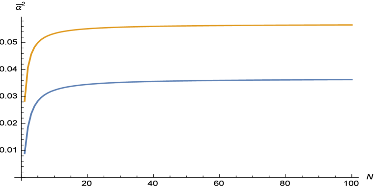
As expected the effect is independent of the number of subintervals $N$. If we consider sufficiently large scales the CMB anisotropy observations give a good estimation of the parameter $\sigma^{2}\approx 10^{-10}$, and since the asymptotic value of $\beta$ is about $0.035$ as shown in fig.(5), we can conclude that the effect is of order unity only for very high redshift $z>10^{5}$, but even in that case the relative error $\sigma_{z_{i}}/z$ would be small and of order $10^{-5}$.

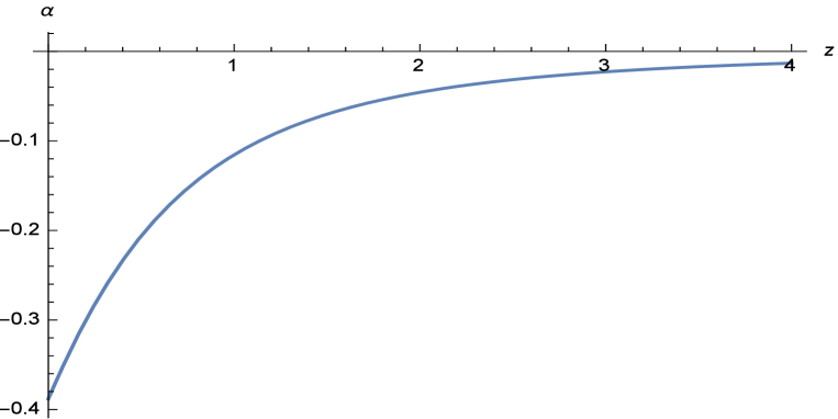
Note that according to eq.(26) $\overline{\alpha}$ depends on $z_{H}$ and is a decreasing function of the redshift. This is due to the fact that $\alpha_{i}$ tends to zero at high redshift because the gravitational potential is frozen in a matter dominated Universe, so that the average through which $\alpha$ is defined in eq.(26) is dominated by the high redshift small values of $\alpha_{i}$.

VII Behavior of $\overline{\alpha}$

In the continuous limit $\alpha_{i}$ is replaced by the function

$$\alpha = \frac{d}{d\eta}\bigg{(}\frac{D(\eta)}{a(\eta)}\bigg{)}=\frac{dz}{d\eta}\frac{d}{dz}\bigg{(}\frac{D(z)}{a(z)}\bigg{)}=-H(z)\frac{d}{dz}\bigg{(}\frac{D(z)}{a(z)}\bigg{)}\,.$$ (33)

For a flat matter dominated Universe, which should be a good model of the late time Universe in the epoch in which the time derivative of the gravitational potential is relevant, the growth factor is given by peebles:1993

$$D(z) = E(z)G(z)$$ (34)

$$G(z) = \frac{5\Omega_{m}}{2}\int^{\infty}_{z}\frac{1+z^{\prime}}{E(z^{\prime})^{3}}dz^{\prime}$$ (35)

$$E(z) = \sqrt{\Omega_{m}(1+z)^{3}+1-\Omega_{m}}\,.$$ (36)

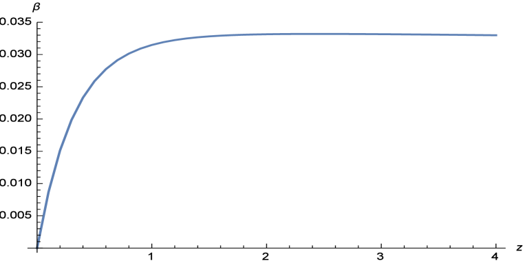
As shown in fig.(4), $D/a$ is asymptotically constant during the matter domination phase, as expected from the freezing of the gravitational potential during that era.

Figure 3: The function $\alpha(z)$ is plotted as a function of the redshift, in units of time of of $H_{0}^{-1}$. As expected it tends to zero a high redshift, where the gravitational potential freezes.

Figure 4: The quantity $\overline{\alpha}^{2}$, as defined in eq.(26), is plotted as a function of the number $N$ of intervals , in units of time of of $H_{0}^{-1}$. The blue curve is for $z_{H}=1$, and the orange curve is for $z_{H}=0.5$. As it can be seen there is convergence for large values of $N$. Also note that $\overline{\alpha}^{2}$ is smaller for larger values of $z_{H}$ because $\alpha$ is asymptotically tending to zero, making the average smaller.

Figure 5: The quantity $\beta$, as defined in eq.(23-24), is plotted as a function of the redshift in units of $H_{0}^{-1}$. As it can be seen there is convergence towards an asymptotic value for large values of $z$ as expected from the fact $\alpha$ is asymptotically vanishing for large $z$.

VIII Probability distribution for the redshift correction

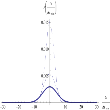
From the above assumptions we can derive the probability distribution of the redshift correction $z_{I}$, due to the spatial variations of the gravitational potential along the line of sight. In this discrete model every space-time configuration along the photon path corresponds to assigning a set of N values to the random variable $\phi_{i}$.

Since as shown in eq.(26) the variance $\sigma_{z_{i}}$ is the same for a set of different $\alpha_{i}$ or for a set of constant $\alpha_{i}=\overline{\alpha}$, we can assume that also the probability distribution could be well approximated under this assumption. Higher momenta could be different but this could be still a useful simplifying hypothesis to compute a probability distribution with the same variance as the one computed using the MGF method.

Let’s call $\{n_{+},n_{-},n_{0}\}$, the number of positive, negative and zero values of the random variable $\psi_{i}$. The corresponding $z_{I}$ will be given by

$$z_{I} = -2(1+z_{H})\overline{\alpha}\Delta r\sigma_{\psi}(n_{+}-n_{-})=\Delta z_{min}S~{},$$ (37)

$$\Delta z_{min} = -2(1+z_{H})\overline{\alpha}\Delta r\sigma_{\psi}~{},$$ (38)

$$S = (n_{+}-n_{-})~{},$$ (39)

where we have introduced $\Delta z_{min}$, the minimum possible inhomogeneous contribution to the total redshift. According to our discrete model the total inhomogeneous redshift is a finite multiple of this minimum contribution, so we get:

$$-N\leq \frac{z_{I}}{\Delta z_{min}} \leq N~{},$$ (40)

where the lower and upper bounds correspond to configurations of all positive or all negative values of $\psi_{i}$, i.e. $n_{+}=N$ or $n_{-}=N$. Since every interval can have three possible values of $\psi_{i}$, we have a total of $3^{N}$ possible different configurations. Because of the fact that what it matters is the sum $(n_{+}-n_{-})$, but not the order in which positive or negative perturbations appear, different space-time configurations can lead to the same value of $z_{I}$. This degeneration is the origin of the intrinsic uncertainty on determining the origin of the total redshift, and consequently to estimate other background cosmological parameters such the $\Omega_{\Lambda}$.

The number of space-time configurations corresponding to a given value of $z_{I}$ can be calculated analytically. Let’s start from the number of configurations corresponding to a given set $\{n_{-},n_{+}\}$ of positive and negative values of $\psi_{i}$, which is is given by:

$$N_{c}(n_{-},n_{+}) = \frac{N!}{n_{-}!n_{+}!(N-n_{-}-n_{+})!}~{}.$$ (41)

For a given $S$ the maximum $n_{+}$ corresponds to configurations with $n_{0}=0$, so from

$$n_{+}+n_{-}+n_{0} = N\,,$$ (42)

$$n_{+}-n_{-} = S\,,$$ (43)

we get

$$n_{+}^{max} = Max[n_{+},S]=\frac{N+S}{2}.$$ (44)

The number of different configurations corresponding to a given value of $z_{I}$, i.e. to a given value of $S=(n_{+}-n_{-})$, can be then computed as

$$N_{S} = \sum_{n_{+}-n_{-}=S}N_{c}(n_{-},n_{+})=\sum^{n_{+}^{Max}}_{n_{+}^{Min}}N_{c}(n_{+}-S,n_{+})=\sum^{(N+S)/2}_{n_{+}=S}N_{c}(n_{+}-S,n_{+})=$$ (46)

$${}_{2}F_{1}\bigg{[}(1+S-N)/2;(S-N)/2;S+1;4\bigg{]}\frac{N!}{S!(N-S)!}\,,$$

where ${}_{2}F_{1}$ is the Gauss hypergeometric function. It is easy to verify that due to the properties of ${}_{2}F_{1}$ $N_{S}$ is symmetric to respect to $S=0$, as expected from the symmetry of the uniform and symmetric probability distribution function $P(\psi)$ from which it is computed.

The formula derived above is consistent with the total number of possible configurations, i.e. we have

$$N_{tot}=\sum^{N}_{S=-N}N_{S} = 3^{N}~{}.$$ (47)

The PDF for S is finally given by

$$P(S)=\frac{N_{S}}{N_{tot}}=3^{-N}{}_{2}F_{1}\bigg{[}(1+S-N)/2;(S-N)/2;S+1;4\bigg{]}\frac{N!}{S!(N-S)!}$$ (48)

which is plotted in fig.(1) for different values of $N$, with $P(S)=P(\frac{z_{I}}{z_{min}})$.

IX Effects on the estimation of background cosmological parameters

We have seen that the dispersion of $z_{I}$ around the central value ($z_{I}=0$), is increasing as N increases, while its average value remains zero because of the symmetry of $P(S)$. The estimation of background cosmological parameters requires to extract $z_{H}$ from the observed redshift $z_{obs}$, but due to our ignorance of the exact configuration of the gravitational potential along the line of sight, the term $z_{I}$ is effectively acting as an error for $z_{H}$, i.e.

$$z_{H} = z_{obs}-z_{I}\,,$$ (49)

$$\sigma_{z_{H}}^{2} = \sigma_{z_{obs}}^{2}+\sigma_{z_{I}}^{2}\,$$ (50)

where $\sigma_{z_{obs}}$ is the systematic observational error on the observed redshift $z_{obs}$. This has a direct consequence on the estimation of any background cosmological parameter based on redshift observations. In general the measurement of any redshift dependent background observable quantity $Q(z_{H})$ will have a propagated error

$$\sigma_{Q}^{2}(z_{H}) \approx \left(\frac{dQ}{dz}\right)^{2}\Big{|}_{z=z_{obs}}\sigma_{z_{I}}^{2}(z_{obs})\,.$$ (51)

Since the function $\sigma_{z_{I}}^{2}(z_{obs})$ is growing monotonically because is proportional to the distance, the uncertainty $\sigma_{Q}(z_{obs})$ may grow or decrease as function of the redshift depending on the behavior of the derivative $dQ/dz$.

X Effects on the luminosity distance

In the following sections we will consider two specific cases related to the effects on the luminosity distance. Note that, following the arguments given in the beginning of section III, we are assuming that the effects on the redshift due to the difference of the peculiar velocity and gravitational potential between the source and the observer can be determined independently using other observations, and can be consequently subtracted from the observed redshift, as done for example for supernovae in Riess:2016jrr , a procedure called redshift correction in that context.

The effects of inhomogeneities on the luminosity distance $D_{L}(z)$ are not only due to the change in the redshift but also to lensing and other integrated effects along the line of sight Sasaki ; Dyer ; Bonvin:2005ps , but here will focus only on the effects due to $z_{I}$ since these are the ones which we considered in this paper. For the other integrated effects terms, which are not due to the background redshift modification, a similar discrete approach could be adopted, but it would go beyond the scope of this paper, which is not the study of the effects of inhomogeneities on the luminosity distance, but more in general the study of the effects on the redshift and the consequences on cosmological observables estimation. Other investigations of the effects of inhomogeneities on the luminosity distance using non discrete approaches based on different averaging procedures applied to cosmological perturbations, including the effects we are not considering here, can be found for example in Fleury:2016fda ; Ben-Dayan:2014swa ; BenDayan:2013gc ; BenDayan:2012ct .

Assuming a flat FRW background model the luminosity distance $D_{L}(z)$ and the comoving distance $r(z)$ are given by

$$r(z) = \int^{z}\frac{dz^{\prime}}{H(z^{\prime})}$$ (52)

$$D_{L}(z) = (1+z)r(z)$$ (53)

and the error on $D_{L}(z)$ due to $z_{I}$ is

$$\sigma_{D}^{2} \approx \left(\frac{dD_{L}}{dz}\right)^{2}\sigma_{z_{I}}^{2}=\left[\frac{(1+z)}{H(z)}+r(z)\right]^{2}\sigma_{z_{I}}^{2}\,.$$ (54)

As explained above the propagated error depends both on $\sigma_{z_{I}}$ and the derivative $D_{L}(z)$, which in this case are both monotonous growing functions of the redshift.

XI Hubble parameter

Let’s consider for example the case of the present value of the Hubble parameter $H_{0}$. The local low redshift estimation of $H_{0}$ is based on the relation Romano:2016utn

$$H_{0}^{loc} = \lim_{z_{H}\to 0}\frac{z_{H}}{D_{L}(z_{H})}\,.$$ (55)

According to the above expression the Gaussian propagated error on $H_{0}^{loc}$ associated to the uncertainty of $z_{H}$ due to $z_{I}$ is

$$\frac{\sigma_{H_{0}}}{H_{0}}\approx\frac{1}{2}H_{0}D_{L}^{\prime\prime}(z_{av})\sigma_{z_{I}}(z_{av})\,.$$ (56)

where $z_{av}$ is the average redshift of the supernovae employed in the analysis. In practice the value of $H_{0}$ is estimated using low redshift supernovae in a finite range Riess:2016jrr , so the effect on the data fitting should be estimated more accurately using a procedure similar to the one given below.

XII Estimation of the cosmological constant

Another interesting case could be the estimation of the cosmological constant using the luminosity distance of high redshift supernovae. In this case the observational data could be binned in different redshift intervals and then for each one of them an error $\sigma_{z_{I}}$ could be estimated using eq.(32). The $\chi^{2}$ variable which is minimized to fit the data is defined as

$$\chi^{2} = \sum^{N}_{j=1}\left(\frac{D^{obs}_{L}(z_{j})-D^{th}_{L}(z_{j})}{\sigma_{z_{j}}}\right)^{2}$$ (57)

where we are denoting with $z_{j}$ the background redshift value $z_{H}$ of the j-th supernova and $\sigma_{z_{j}}$ is given in eq.(50).

The inclusion of the redshift dependent error given in eq.(50) in the data analysis is expected to have some effect on the estimation of $\Omega_{\Lambda}$ which only a careful analysis of observational data can quantify, and we leave it to a future work.

XIII Conclusions

We have developed a discrete model to account for the effects of inhomogeneities on the redshift of photons. Using this model we have computed the probability distribution of the redshift correction with respect to the background value obtaining that its dispersion is proportional to the square root of the comoving distance.Observational data analysis should include this contribution to the total error budget, which depends on the distance of the source. We then considered what are the general implications for the estimation of background cosmological parameters, and gave some examples for the case of quantities related to the luminosity distance such as the Hubble parameter and the cosmological constant.

The model correctly reproduces discretely the expected stochastic properties of the propagation of photons in inhomogeneous media and could be particularly suitable for the numerical estimation of the effects of inhomogeneities on cosmological observables using Montecarlo methods. A more accurate treatment could involve the use of discrete random variables following other different physically motivated probability distributions.

In the future it will be interesting to compare the predictions based on this discrete approach to the results of numerical calculations for the propagation of photons in inhomogeneous media, in particular to determine the parameter $\beta$.

XIV Acknowledgments

I thank Gabriele Veneziano for helpful discussions. I am also grateful to the theoretical division of CERN and the College du France for their hospitality.

References

- (1) A. E. Romano, arXiv:1609.04081 [astro-ph.CO].
- (2) A. G. Riess et al., Astrophys. J. 826, no. 1, 56 (2016) doi:10.3847/0004-637X/826/1/56 [arXiv:1604.01424 [astro-ph.CO]].
- (3) Lumsden, S. L., Heavens, A. F., & Peacock, J. A. 1989, MNRAS , 238, 293
- (4) S. Zaroubi, M. Viel, A. Nusser, M. Haehnelt and T.-S. Kim, Mon. Not. Roy. Astron. Soc. 369, 734 (2006) doi:10.1111/j.1365-2966.2006.10333.x [astro-ph/0509563].
- (5) P. J. E. Peebles, Principles of physical cosmology (Princeton University Press, 1993).
- (6) S. A. Vallejo and A. E. Romano, arXiv:1703.08895 [astro-ph.CO].
- (7) Lloyd, K.H., http://dspace.dsto.defence.gov.au/dspace/handle/1947/8810.
- (8) E. W. Kolb, S. Matarrese and A. Riotto, arXiv:astro-ph/0506534.
- (9) T. Buchert, arXiv:gr-qc/0509124, and references therein.
- (10) Y. Nambu and M. Tanimoto, arXiv:gr-qc/0507057.
- (11) A. Ishibashi and R. M. Wald, arXiv:gr-qc/0509108.
- (12) K. Tomita, Mon. Not. Roy. Astron. Soc. 326, 287 (2001).
- (13) A. E. Romano and S. A. Vallejo, Eur. Phys. J. C76, 216 (2016), arXiv:1502.07672.
- (14) A. E. Romano and P. Chen, JCAP 1110, 016 (2011), arXiv:1104.0730.
- (15) A. E. Romano and S. A. Vallejo, Europhys. Lett. 109, 39002 (2015), arXiv:1403.2034.
- (16) A. E. Romano, Int. J. Mod. Phys. D21, 1250085 (2012), arXiv:1112.1777.
- (17) M. Sasaki, Mon. Not. R. Astron. Soc. 228, 653 (1987).
-
(18)
C. C. Dyer and R. C. Roeder, Astrophys. J. 174, L115 (1972);
C. C. Dyer and R. C. Roeder, Astrophys. J. 180, L31 (1973);
C. C. Dyer and R. C. Roeder, Astrophys. J. 189, 167 (1974);
T. Futamase and M. Sasaki, Phys. Rev. D40, 2502 (1989);
M. Kasai, T. Futamase and F. Takahara, Phys. Lett. A 147, 97 (1990);
R. Kantowski, Astrophys. J. 507, 483 (1998);
N. Sugiura, N. Sugiyama and M. Sasaki, Prog. Theo. Phys., 101, 903 (1999);
T. Pyne and M. Birkinshaw, Mon. Not. R. Astron. Soc. 348, 581 (2004). - (19) C. Bonvin, R. Durrer and M. A. Gasparini, Phys. Rev. D 73, 023523 (2006) [Erratum-ibid. D 85, 029901 (2012)] [astro-ph/0511183].
- (20) I. Ben-Dayan, M. Gasperini, G. Marozzi, F. Nugier and G. Veneziano, Phys. Rev. Lett. 110, no. 2, 021301 (2013) doi:10.1103/PhysRevLett.110.021301 [arXiv:1207.1286 [astro-ph.CO]].
- (21) I. Ben-Dayan, M. Gasperini, G. Marozzi, F. Nugier and G. Veneziano, JCAP 1306, 002 (2013) doi:10.1088/1475-7516/2013/06/002 [arXiv:1302.0740 [astro-ph.CO]].
- (22) I. Ben-Dayan, R. Durrer, G. Marozzi and D. J. Schwarz, Phys. Rev. Lett. 112, 221301 (2014) doi:10.1103/PhysRevLett.112.221301 [arXiv:1401.7973 [astro-ph.CO]].
- (23) P. Fleury, C. Clarkson and R. Maartens, JCAP 1703, no. 03, 062 (2017) doi:10.1088/1475-7516/2017/03/062 [arXiv:1612.03726 [astro-ph.CO]].