Matrix geometries and Matrix Models

Abstract

We study a two parameter single trace $3$-matrix model with $SO(3)$ global symmetry. The model has two phases, a fuzzy sphere phase and a matrix phase. Configurations in the matrix phase are consistent with fluctuations around a background of commuting matrices whose eigenvalues are confined to the interior of a ball of radius $R=2.0$. We study the co-existence curve of the model and find evidence that it has two distinct portions one with a discontinuous internal energy yet critical fluctuations of the specific heat but only on the low temperature side of the transition and the other portion has a continuous internal energy with a discontinuous specific heat of finite jump. We study in detail the eigenvalue distributions of different observables.

1 Introduction

One of the most striking and interesting features of multi-matrix models is the phenomenon of emergent geometry. The notion of classical geometry changes drastically within the context of matrix models; the geometry is no longer a basic concept which exists a priori but instead it emerges dynamically as a consequence of the reordering of degrees of freedom. This is in many ways exciting because matrix models can lead to new ways of thinking about the structure of the space time.

The interest in matrix models has grown since it was suggested that they might provide a non-perturbative definition for M theory [1]. Several kinds of matrix models have been proposed for this purpose [1, 2, 3]. The IIB matrix model (IKKT model) [2] is one of these proposals; it is a large $N$ reduced model [4] of ten-dimensional supersymmetric Yang-Mills theory and the action is a matrix regularised form of the Green-Schwarz action of the IIB superstring. It is postulated that it gives a constructive definition of type IIB superstring theory.

Finite dimensional matrix models have also been used to regulate field theories [7, 8, 9, 10, 11, 12, 13] and diverse fully non-perturbative numerical studies have been performed, see for instance [14, 15, 16, 17, 18, 19, 20].

The pure commutator action, which we refer to as the Yang-Mills matrix model, is also particularly interesting since in $d=10,6$ and $4$ dimensions it corresponds to the bosonic part of the IKKT model. The model is well defined in dimensions $d>2$ and matrix size $N>3$ [29]. In dimension $d=2$ the model, with a quadratic term is added to stabilise it, is exactly solvable [24, 32]. These bosonic Yang-Mills matrix models in different dimensions have been considered as possible realizations of emergent geometry/gravity [30].

Numerical studies of pure Yang-Mills matrix models were performed in [4] for different dimensions (numbers of matrices) and more recently in [5, 6] it is argued that perturbation theory around a background of commuting matrices gives a good approximation to the 3-dimensional model. In [6] based on a two loop computation it is predicted that the eigenvalues of the background commuting matrices are uniformly distributed within a ball of radius $R\sim 1.8$ which is in broad agreement with our findings here.

Our starting point is an action in which the basic objects are simple Hermitian matrices; no geometrical background is assumed a priori. The model describes the statistical fluctuations of matrices with prescribed energy functional. The geometry arises as a condensate around which the system fluctuates. Generically, multi-matrix models can undergo transitions between different geometries and phases with no geometrical content. Given the novelty of these phenomena it is worth studying the simplest model that exhibits such phenomena in detail.

The simplest model in which a geometry has been shown to be emergent is a 3-matrix model consisting of the trace of the square of the commutator of the matrices (a Yang-Mills term) plus the epsilon-tensor contracted with the trace of the three matrices (a Myers term)[22]. This model was studied in [15, 17, 19, 20] and is a static bosonic subsector of the BMN model [3].

The model exhibits a geometrical phase for sufficiently large coupling to the cubic Myers term, with the geometry being that of a fuzzy sphere [23, 24]; a non-commutative [31] version of the commutative sphere [33].

At a critical coupling, which can be traded for a critical temperature, a phase transition occurs and the condensed geometry evaporates. In the geometrical, low temperature phase, small fluctuations around this condensate correspond to a $U(1)$ gauge and scalar field multiplet [13, 25, 20].

The model can be extended by adding appropriate potentials in order to enhance the range of parameters in which the fuzzy sphere phase is stable [20]. The general phase diagram for a class of such models was predicted in [20], one of the purposes of this paper is to check these predictions in detain in a non-perturbative study. We find that indeed the phase diagram is well predicted by theoretical expressions presented in [20].

Manifolds in higher dimensions can emerge from more general matrix models with essentially the same structure and phenomenology as can be seen in [26, 27, 28].

In the current paper we study, in detail, the high temperature phase of the model and establish that this phase is consistent with the three matrices fluctuating around commuting matrices where the eigenvalues of the commuting matrices are confined to the interior of a solid three dimensional ball. The fluctuations are still significant as the commutator of pairs of matrices is itself a peaked (almost triangular) distribution.

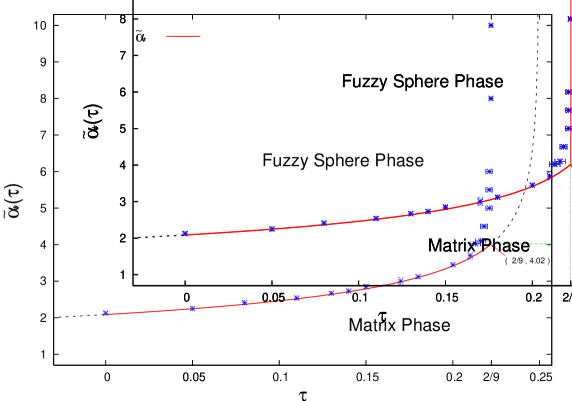
We concentrate on the effect of adding a quadratic, mass like perturbation to the 3-matrix model. We find that below a critical temperature any negative massive perturbation induces a transition from the matrix phase to the fuzzy sphere phase. For higher temperatures a more negative quadratic coupling is necessary. The phase diagram, which is one of the principal results of this paper, is shown in figure 3.

• We find the ground states of the system are characterised by either the $N$ dimensional irreducible representation of $SU(2)$ (the fuzzy sphere phase) or a continuum spectrum (matrix phase) for one of the matrices. These characterize the two phases of the system. Though meta stable states other than the irreducible fuzzy sphere are present in the system they never correspond to the true ground state, they do however appear stable in the large $N$ limit where tunneling is suppressed.

• We study the phase diagram (see figure 3) as a function of the two parameters $\tau$ and $\tilde{\alpha}$ and locate the co-existence curve with some precision.

• The co-existence curve rapidly asymptotes to the special line $\tau=\frac{2}{9}$ where the energy functional defining the model becomes a complete square.

• We found evidence for two distinct types of transition in the emergent geometry scenario: for $0<\tau<\frac{2}{9}$, as the transition is approached from the fuzzy sphere phase with fixed $\tau$, the system has a divergent specific heat with critical exponent $\alpha=\frac{1}{2}$ while crossing the phase boundary for fixed $\tilde{\alpha}>4.02$ there appear to be no critical fluctuations and the transition is one with a continuous internal energy and discontinuous specific heat.

• We find that a useful description of the matrix phase is in terms of fluctuations about a background of commuting matrices whose eigenvalues are concentrated in a three dimensional ball of radius $R=2.0$.

The paper is structured as follows: Section 2 describes the model and the predictions of the phase diagram from the effective potential [20] in the fuzzy sphere phase. Section 3 describes the matrix phase and the consequences of a background of commuting matrices with eigenvalues uniformly distributed within a ball. Section 4 describes our numerical results and section 5 contains our conclusions.

2 The model

We begin by considering an action functional built as a single trace quartic polynomial of 3 Hermitian matrices with $SO(3)$ symmetry. There are four available invariants:

$$\;\mbox{Tr}\;D_{a}D_{b}D_{a}D_{b},\;\;\;\;\;\mbox{Tr}\;(D_{a}^{2})^{2},\;\;\;\;\;\mbox{Tr}\;i\epsilon_{abc}D_{a}D_{b}D_{c},\;\;\;\;\;\mbox{Tr}\;D_{a}^{2}.$$ (1)

In this paper we restrict our study to the two parameter model given by the action

$$S[D]=\frac{\tilde{\alpha}^{4}}{N}Tr\left[-\frac{1}{4}[D_{a},D_{b}]^{2}+\frac{i}{3}{\epsilon}_{abc}[D_{a}D_{b}]D_{c}+\tau D_{a}^{2}\right]\ ;$$ (2)

where stability of the model requires the $\tau>0$. For $\tau<0$ the action for commuting matrices is unbounded from below. The most general model would include in addition $Tr(D_{a}^{2})^{2}$ with an extra coupling.

The action (2) is invariant under unitary transformations $U(N)$, $D_{a}\to UD_{a}U^{\dagger}$ and global $SO(3)$ rotations of the matrices. The modes $c_{a}=Tr(D_{a})$ decouple from the others and we therefore choose to work with traceless matrices, $Tr\;D_{a}=0$. The parameters of the model are $\tau$ and $\tilde{\alpha}$. $\tilde{\alpha}$ can be identified either as the Yang-Mills coupling constant $g^{2}\equiv\tilde{\alpha}^{-4}$ or the temperature $T\equiv\tilde{\alpha}^{-4}$ [20].

Saddle points of the action, derived from the condition $\delta S=0$, are given by solutions of

$$[D_{b},iF_{ab}]+2\tau D_{a}=0,\qquad\mbox{with}\quad F_{ab}=i[D_{a},D_{b}]+\epsilon_{abc}D_{c}$$

and include the trivial solution $D_{a}=0$ and $D_{a}=\phi J_{a}$ where $J_{a}$ are representations of $SU(2)$, not-necessarily irreducible. For $D_{a}=\phi J_{a}$, then $F_{ab}=-(\phi^{2}-\phi)\epsilon_{abc}J_{c}$ we get an algebraic equation for $\phi$ given by

$$(\phi^{3}-\phi^{2}+\tau\phi)=0$$ (3)

the explicit solutions are

$$\phi=\{\phi_{0},\phi_{-},\phi_{+}\}=\left\{0,\frac{1+\sqrt{1-4\tau}}{2},\frac{1-\sqrt{1-4\tau}}{2}\right\}.$$ (4)

The first corresponds to $D_{a}=0$ and is the ground state of the system for $\tau>\frac{1}{4}$, is a local minimum for $\frac{1}{4}>\tau>0$ and though it appears to be a local maximum for $\tau<0$, the model has no ground state for such value of $\tau$. The second solution gives the local minima $D_{a}=\phi_{-}J_{a}$, for $\tau<\frac{1}{4}$. These minima $D_{a}=0$ and $D_{a}=\phi_{-}J_{a}$ are separated by a potential barrier whose highest point is localised at the local maximum $\phi_{+}$. As $\tau$ approaches zero $\phi_{-}\rightarrow 1$, which corresponds to the case for $m^{2}=\tau=0$ studied in [15, 19, 20]. For arbitrary $\tau$ has been also studied by other authors [21, 20].

For the configurations $D_{a}=\phi J_{a}$ the action

$$S[D]=V_{class}(\phi)=\frac{2}{N}\sum_{i}n_{i}C_{2}(n_{i})\;\tilde{\alpha}^{4}\left(\frac{\phi^{4}}{4}-\frac{\phi^{3}}{3}+\frac{\tau\phi^{2}}{2}\right)$$ (5)

where $C_{2}(n_{i})$ is the Casimir of the representation of dimension $n_{i}$ and $\sum_{i}n_{i}=N$. For $\tau<\frac{2}{9}$ the potential $V_{class}(\phi_{-})<0$ and the configurations $D_{a}=\phi_{-}J_{a}$ is of lower energy than $D_{a}=0$, which is zero. The configuration with minimum energy is then given by maximising the sum of Casimirs, this is achieved by $J_{a}=L_{a}$, where $L_{a}$ is the irreducible representation of dimension $N$. For $\tau=\frac{2}{9}$ we have $V_{class}(\phi_{-})=0$ and the configurations $D_{a}=0$ and $D_{a}=\phi_{-}J_{a}$, with any representation $J_{a}$, become degenerate. Figure 1 shows the potential (5) for different $\tau$.

Therefore the classical prediction is that for $\tau<\frac{2}{9}$, and any value of $\tilde{\alpha}$ the ground state is $D_{a}=\phi_{-}L_{a}$ and small fluctuations around this configuration have the geometrical content of a Yang-Mills and scalar multiplet on a background fuzzy sphere.

The parameter domain $\frac{2}{9}<\tau<\frac{1}{4}$ is of special interest. The classical analysis above suggests that the fuzzy sphere is unstable here, however, since the potential still has a local minimum and in the $N\rightarrow\infty$ limit all representations such that $\frac{1}{N}\sum_{i}n_{i}C_{2}(n_{i})\rightarrow 0$ become degenerate with the $D_{a}=0$ configuration one might wonder if one of these configurations gives the ground state of the system when fluctuations are included or perhaps as suggested by the analysis of [20] and discussed in the next section, the fuzzy sphere phase is stabilised by fluctuation. The answer as we will see, is that numerical simulations do not support the assertion that the fuzzy sphere is stabilised in this parameter range, but rather that the coexistence curve between the fuzzy sphere phase and the matrix phase asymptotes to the line $\tau=\frac{2}{9}$.

For $\tau=\frac{2}{9}$ the model is indeed special, the action is always positive semi-definite and can be written in the form

$$S[D]=\frac{\tilde{\alpha}^{4}}{N}Tr\left(\frac{i}{2}[D_{a},D_{b}]+\frac{1}{3}\epsilon_{abc}D_{c}\right)^{2},$$ (6)

from which we see that $D_{a}=0$ and the orbit $D_{a}=U\frac{2}{3}L_{a}U^{\dagger}$ have zero action.

Figure 1: Classical potential for different values of $\tau$ for fixed $\tilde{\alpha}=5$.

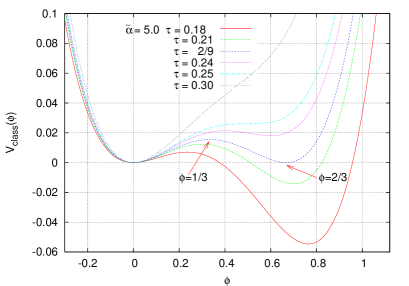
2.1 Quantum corrections and critical behaviour

In the previous section we described the classical potential predictions for the phase transition by choosing $D_{a}=\phi L_{a}$ and studying the potential for $\phi$. This analysis suggests that $\phi$ plays the role of order parameter for the transitions which are taking place in the model. We will now take into account the quantum fluctuations. The computation of the quantum effective action and the quantum effective potential was carried out in detail [25, 19] for a more general $SO(3)$ globally invariant matrix model. The results there correspond to the present case by setting $m^{2}=0$.

Using the standard background field method around the classical configuration $D=\phi L_{a}$ one finds the effective potential in the large $N$ limit is given by

$$\frac{V_{\rm eff}}{2C_{2}}=\tilde{\alpha}^{4}\left[\frac{\phi^{4}}{4}-\frac{\phi^{3}}{3}+\tau\frac{\phi^{2}}{2}\right]+\log\phi^{2}$$ (7)

As discussed in [25, 19] the phase diagram including fluctuations is obtained from the minimum of this effective potential. Due to the log term the effective potential (7) is not bounded from below near $\phi=0$ and since in its derivation it was assumed that we were expanding around $D_{a}=\phi L_{a}$ it is only valid where such a ground state exists.

The minimum is therefore one of the roots of the polynomial $\phi\frac{\partial V_{\rm eff}(\phi)}{\partial\phi}=0$ which gives the equation

$${\phi}^{4}-{\phi}^{3}+\tau{\phi^{2}}+\frac{2}{\tilde{\alpha}^{4}}=0,$$ (8)

and determines $\phi$ in $D_{a}=\phi L_{a}$ at quantum level. Explicitly the minimum is given by

$${\phi}=\frac{1}{4}+\frac{1}{2}\sqrt{\frac{1}{4}-\frac{2\tau}{3}+d}+\frac{1}{2}\sqrt{\frac{1}{2}-\frac{4\tau}{3}-d+\frac{1-4\tau}{4\sqrt{\frac{1}{4}-\frac{2\tau}{3}+d}}},$$ (9)

with the definitions

$$q=1-\frac{8\tau}{3}+\frac{\tilde{\alpha}^{4}\tau^{3}}{27},\;\;\;p=q^{2}-\frac{(\frac{8}{3}+\frac{\tilde{\alpha}^{4}\tau^{2}}{9})^{3}}{\tilde{\alpha}^{4}},\;\;\;\;d=a^{-\frac{4}{3}}\bigg{(}\big{(}q+\sqrt{p}\big{)}^{\frac{1}{3}}+\big{(}q-\sqrt{p}\big{)}^{\frac{1}{3}}\bigg{)}.$$ (10)

Figure 2: (a) Effective potential for different values of $\tau$ for $\tilde{\alpha}=5$. (b) Effective potential for $\tau=0.18$ for different values of $\tilde{\alpha}$

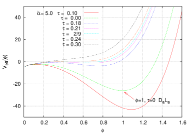
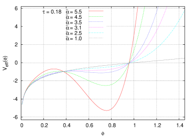
$V_{\rm eff}$ is plotted in figure 2. In figure 2(a) the potential is shown for a fixed value of $\tilde{\alpha}=5$ for different values of $\tau$. In figure 2(b) we fix the value of $\tau=0.18$ varying $\tilde{\alpha}$. From both pictures we can see that there exists a region in which the fuzzy sphere ceases to exist. This means that there exists a critical coexistence curve in the $(\tau,\tilde{\alpha})$ plane where the model undergoes a phase transition between the two phases.

These expressions predict that for sufficiently large $\tilde{\alpha}$ or low temperature and $\tau<\frac{1}{4}$ the fuzzy sphere is the ground state of the model. The local minimum disappears for the simultaneous solution of $V_{\rm eff}^{\prime}(\phi)=0$ and $V_{\rm eff}^{\prime\prime}(\phi)=0$ so that

$$4\phi^{2}_{*}-3\phi_{*}+2\tau=0$$ (11)

which gives the critical values for $\phi$ and $\tilde{\alpha}$.

$$\phi_{*}=\frac{3}{8}\left(1+\sqrt{1-\frac{32\tau}{9}}\right)\quad\hbox{ and}\quad g_{*}^{2}=\frac{1}{\tilde{\alpha}_{*}^{4}}=\frac{{\phi}_{*}^{2}({\phi}_{*}-2\tau)}{8}.$$ (12)

These equations defines the phase diagram $(\tau,\tilde{\alpha})$ for the present model. They prediction that at zero temperature i.e. $\tilde{\alpha}=\infty$ where $\phi_{*}=1/2$ and $\tau=1/4$.

The phase diagram is presented in Figure 3 together with a comparison with numerical simulations. Numerical results are in excellent agreement with the prediction from effective potential for $\tau<\frac{2}{9}$ where the coexistence curve predicted in (12) clearly delimits the fuzzy sphere phase from the matrix phase. The fuzzy sphere exists for $\tilde{\alpha}>\tilde{\alpha}_{*}$ and for $\tau<\tau_{*}$, where $\tau_{*}(\tilde{\alpha})$ is obtained by inverting (12).

However, for $\frac{1}{4}>\tau>\frac{2}{9}$, simulations show that the coexistence curve asymptotes rapidly to the line $\tau=\frac{2}{9}$ for $\tilde{\alpha}$ greater than the special value $\tilde{\alpha}_{*}=12\left(\frac{4}{107+51\sqrt{17}}\right)^{1/4}\sim 4.02$. As we cross the critical value of $\tilde{\alpha}$, a rather exotic phase transition occurs where the geometry disappears as the temperature is increased. In the high temperature phase, which we call a matrix phase, the order parameter $\phi$ goes to zero as $N^{-1}$. In this phase the fluctuations are insensitive to the value of $\tilde{\alpha}$, they are in fact fluctuations around commuting matrices. Since, in the large $N$ limit, $\tilde{\alpha}$ is unimportant we can rescale the matrices to eliminate $\tilde{\alpha}$ from the quadratic term, defining $X_{a}=\frac{\tilde{\alpha}}{\sqrt{N}}D_{a}$, we obtain

$$S[X]=NTr(-\frac{1}{4}[X_{a},X_{b}]^{2}+\frac{2i\tilde{\alpha}}{3\sqrt{N}}\epsilon_{abc}X_{a}X_{b}X_{c}+\frac{\tilde{\alpha}^{2}\tau}{N}X_{a}^{2})$$ (13)

and see that in this rescaled model both $\tau$ and $\tilde{\alpha}$ drop out of the model in the large $N$ limit.

Figure 3: Phase diagram $(\tau,\tilde{\alpha})$. The solid line corresponds to the theoretical prediction eq.(12) for $\tau<\tau_{*}=\frac{2}{9}$. The numerical points are obtained from simulations with matrix sizes $N=19,N=24,N=35$ and $N=64$. We see some rounding of the coexistence curve near $(\tilde{\alpha}_{*}=4.02,\;\tau=\frac{2}{9})$, before it asymptotes to the line $\tau=\frac{2}{9}$.

Next we discuss the numerical results which include the eigenvalue distributions for the configurations.

2.2 Specific heat and phase transitions.

There are several useful general identities that we can derive between expectation values of observables, the simplest of these is the relation between different components of the action. Since our action is a polynomial in the matrices $X_{a}$ it can be expressed as $S=S_{4}+S_{3}+S_{2}$ where $S_{k}[\lambda X]=\lambda^{k}S[X]$. Then if we scale the fields $X_{a}\rightarrow\lambda X_{a}$ in both the action and the measure, the partition function $Z$, is invariant and under an infinitesimal rescaling we obtain the constraint

$$4<S_{4}>+3<S_{3}>+2<S_{2}>=3(N^{2}-1),$$ (14)

which allows us to eliminate $<S_{4}>$. Defining ${\cal S}_{k}=\frac{<S_{k}>}{N^{2}}$ we have for large $N$ obtain

$${\cal S}=\frac{3}{4}+\frac{1}{4}{\cal S}_{3}+\frac{1}{2}{\cal S}_{2}.$$ (15)

For our model, with

$$X_{a}=\frac{\tilde{\alpha}}{\sqrt{N}}D_{a},$$ (16)

we have

$$S_{4} = -\frac{N}{4}\;\mbox{Tr}\;([X_{a},X_{b}]^{2}),$$ (17)

$$S_{3} = N\frac{2}{3}i\alpha\epsilon_{abc}\;\mbox{Tr}\;(X_{a}X_{b}X_{c}),$$ (18)

$$S_{2} = N\alpha^{2}\tau\;\mbox{Tr}\;(X^{2}_{a}).$$ (19)

Where $\alpha=\frac{\tilde{\alpha}}{\sqrt{N}}$. In the fuzzy sphere phase we know fluctuations are around the configuration $D_{a}=\phi L_{a}$ and we then have the predictions (see [20] for details) the partition function $Z={\rm e}^{-F}$ with the free energy $F$ given by

$$F(\tilde{\alpha},\tau)=\frac{V_{\rm eff}}{N^{2}}+3\ln\tilde{\alpha}.$$ (20)

where $V_{\rm eff}$ is evaluated with $\phi$ given by (9). From this we can then identify

$$\frac{<S_{2}>}{N^{2}}=\frac{\tau\tilde{\alpha}^{4}\phi^{2}}{4},\qquad\frac{<S_{3}>}{N^{2}}=-\frac{\tilde{\alpha}^{4}\phi^{3}}{6}\qquad\frac{<S_{4}>}{N^{2}}=\frac{3}{4}-\frac{\tilde{\alpha}^{4}\tau\phi^{2}}{8}+\frac{\tilde{\alpha}^{4}\phi^{3}}{8}$$ (21)

In particular for the average of the action ${\cal S}$ and the specific heat $C_{v}=\frac{1}{N^{2}}<(S-<S>)^{2}>$ we have

$${\cal S}=\frac{3}{4}+\frac{\tilde{\alpha}^{4}\tau\phi^{2}}{8}-\frac{\tilde{\alpha}^{4}\phi^{3}}{24}\qquad\hbox{and }\qquad C_{v}=\frac{3}{4}+\frac{\tilde{\alpha}^{5}}{32}\phi(\phi-2\tau)\frac{d\phi}{d\tilde{\alpha}}.$$ (22)

3 The Matrix Phase

In terms of $X_{a}$ of (16) the model (2) becomes

$$S[X]=N\;\mbox{Tr}\;\left[-\frac{1}{4}[X_{a},X_{b}]^{2}+\frac{i}{3}\frac{\tilde{\alpha}}{\sqrt{N}}{\epsilon}_{abc}[X_{a}X_{b}]X_{c}+\tau\frac{\tilde{\alpha}^{2}}{N}X_{a}^{2}\right].$$ (23)

We see that at high temperature where $\tilde{\alpha}\rightarrow 0$, provided fluctuations in $X_{a}$ do not grow too rapidly with either $\tilde{\alpha}$ or $N$ then in the large $N$ limit the model reduces to the pure Yang-Mills term

$$S[X]=-\frac{N}{4}\;\mbox{Tr}\;[X_{a},X_{b}]^{2}.$$ (24)

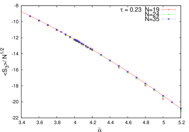
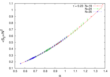
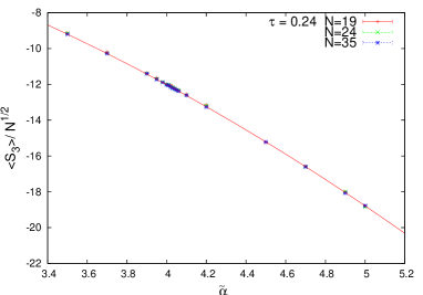
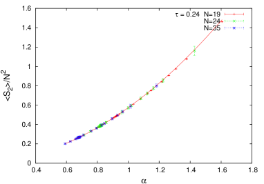
Our numerical results support this and we find that $<\frac{TrX_{a}^{2}}{N}>$ and $\frac{2}{3}\tilde{\alpha}\epsilon_{abc}<Tr(X_{a},X_{b}X_{c})>$ are independent of $N$, see Figures 4.

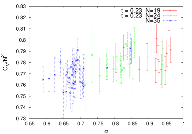
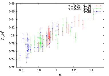
We see immediately from (15) and the reduction to (24) that in the high temperature, matrix phase we should expect both ${\cal S}=\frac{3}{4}=C_{v}$ irrespective of the value of $\tilde{\alpha}$ and $\tau$. This is in accordance with our numerical results shown in Figures 5 and 7 and the earlier results of [20], but there is some discrepancy with Figure 6 which we believe is due to finite size effects as discussed below.

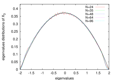
It is argued in [5, 6] that fluctuations are about a background of commuting matrices whose eigenvalues are uniformly distributed in the interior of a solid ball in ${\mathbb{R}}^{3}$. This in turn predicts that the eigenvalue distribution of a single matrix, say $X_{3}$, is the parabolic distribution

$$\rho(x)=\frac{3}{4R^{3}}(R^{2}-x^{2}).$$ (25)

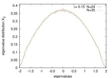
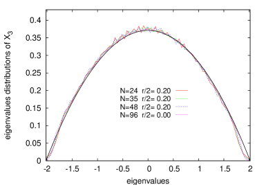
In [6], based on a two-loop approximation, it was estimated that $R\sim 1.8$. This is in reasonable agreement with our numerical results (see Fig 13) which give $R=2.0$. In Figure 13 we can see that the numerical results for the eigenvalue distribution of $X_{3}$ are very well fit by the parabola (25).

Figure 4: $\frac{<S_{3}>}{N^{1/2}}$ as a function of $\tilde{\alpha}$ and $\frac{<S_{2}>}{N^{2}}$ as a function of $\alpha$ for $\tau=0.23,0.24$. We observe collapsed data in both plots in the range showed.

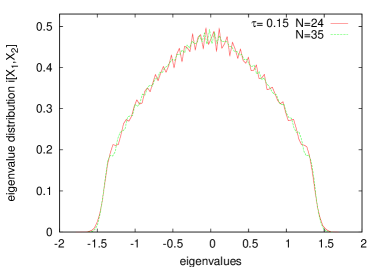
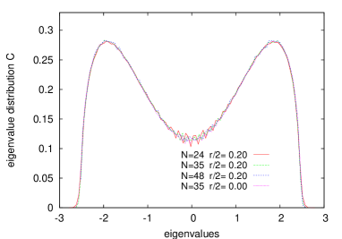
In the same figure we present the distribution for the commutator $i[X_{1},X_{2}]$ showing a symmetric distribution with support lying in the interval $[-1.5,1.5]$. This indicates, that the fluctuations around this background are non-commuting variables.

If we accept the parabolic distribution (25) and radius $R=2$ we can predict

$$<\frac{\;\mbox{Tr}\;}{N}(X^{2}_{a})>=3\int^{R}_{-R}dx_{1}\rho(x_{1})x^{2}_{1}=\frac{3R^{2}}{5}=\frac{12}{5}.$$ (26)

Therefore we have

$${\cal S}_{2} = \alpha^{2}\tau\frac{<\;\mbox{Tr}\;X^{2}_{a}>}{N}=\tau\frac{\tilde{\alpha}^{2}}{N}\frac{12}{5},$$ (27)

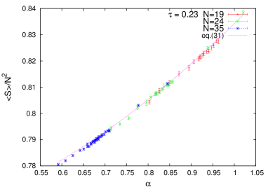
which goes to zero for fixed $\tilde{\alpha}$ in the large $N$ limit. Our numerical results are in very good agreement with this result for $\mathcal{S}_{2}$, as we can see in figure 4 (right). The value of the radius extracted from here is $R=2.01$, in accordance with the value obtained from the eigenvalues of $X_{3}$. However, as $\tilde{\alpha}$ increases we can observe small deviations. The value $R=2$ corresponds to the limit of infinite temperature and large $N$.

From our numerical simulations we see that ${\cal S}_{3}$ goes to zero even more rapidly than ${\cal S}_{2}$. In figure 4 we see that the curves for different $N$ collapse when we

$$\frac{<S_{3}>}{N^{1/2}}=\left<\frac{2}{3}i\tilde{\alpha}\epsilon_{abc}\;\mbox{Tr}\;X_{a}X_{b}X_{c}\right>$$ (28)

as a function of $\tilde{\alpha}$. For different values of $\frac{2}{9}<\tau<\frac{1}{4}$ we find $\frac{S_{3}}{\tilde{\alpha}}$ behaves linear in $\tilde{\alpha}$, however the approximation becomes poorer as $\tau\to\frac{1}{4}$ and higher corrections subleading in $N$ should be taken into account. The data for $\tau=0.23$ is well fit by

$$\frac{<S_{3}>}{N^{1/2}}=0.142533\;\tilde{\alpha}-0.799823\;\tilde{\alpha}^{2},\qquad\qquad\frac{<S_{2}>}{N^{2}}=0.557965\;\alpha^{2}.$$ (29)

For $\tau=0.24$ we find

$$\frac{<S_{3}>}{N^{1/2}}=0.0243563\;\tilde{\alpha}-0.757264\;\tilde{\alpha}^{2},\qquad\qquad\frac{<S_{2}>}{N^{2}}=0.574869\;\alpha^{2}$$ (30)

From which we deduce that ${\cal S}_{3}\rightarrow 0$ as $N^{-\frac{3}{2}}$.

Taking this into account we can write the expectation value of the action $\frac{<S>}{N^{2}}$ given by eq. (15)

$${\cal S} = \frac{3}{4}+\frac{1}{4N}(0.142533\;\tilde{\alpha}-0.799823\;\tilde{\alpha}^{2})+\tau\frac{\tilde{\alpha}^{2}}{N}\frac{6}{5}$$ (31)

$$= \frac{3}{4}+\frac{1}{4N^{1/2}}(0.142533\;\alpha)-\frac{1}{4}(0.799823\;\alpha^{2})+\tau\alpha^{2}\frac{6}{5};\qquad\mbox{for}\;\;\tau=0.23,$$

$${\cal S} = \frac{3}{4}+\frac{1}{4N}(0.024356\;\tilde{\alpha}-0.757264\;\tilde{\alpha}^{2})+\tau\frac{\tilde{\alpha}^{2}}{N}\frac{6}{5}$$ (32)

$$= \frac{3}{4}+\frac{1}{4N^{1/2}}(0.024356\;\alpha)-\frac{1}{4}(0.757264\;\alpha^{2})+\tau\alpha^{2}\frac{6}{5};\qquad\mbox{for}\;\;\tau=0.24,$$

$${\cal S} = \frac{3}{4}+\frac{1}{4N^{1/2}}(-0.159707\;\alpha)-\frac{1}{4}(0.701843\;\alpha^{2})+\tau\alpha^{2}\frac{6}{5};\qquad\mbox{for}\;\;\tau=0.25.$$ (33)

The expectation values for the action $\mathcal{S}$ are shown in figure 8 for these last two particular values of $\tau$.

4 Numerical Results

We now describe the results of the numerical results for the expectation value of the action $<S>$ and the specific heat $C_{v}/N^{2}=<(S-<S>)^{2}>$ as function of $\tilde{\alpha}$ for a fixed value of $\tau$.

Figure 5: The specific heat $C_{v}$ as a function of $\tilde{\alpha}$ for different $\tau$ values, $\tau<2/9$. The curve dashed line corresponds to expression (22) for the specific heat.

Figure 6: Observables $<S>,C_{v}$ for $\tau=0.25$. The range of $\alpha$ shown corresponds to $\tilde{\alpha}<3.7$

Figure 7: Observables $<S>,C_{v}$ as function of $\tau$ for $\tilde{\alpha}=5$. The transition occurs at $\tau=0.219\pm 0.005$.

Figure 8: Expectation value of the action $<S>$ and specific heat $C_{v}$ for $\tau=0.23,0.24$ as a function of $\alpha=\tilde{\alpha}/\sqrt{N}$. These values of $\tau$ lie in the matrix phase.

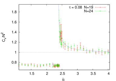
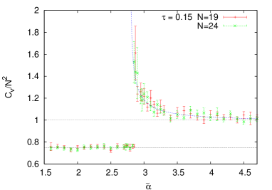
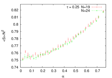
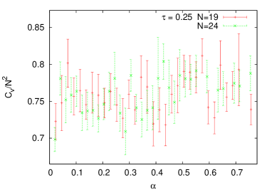
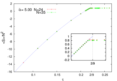
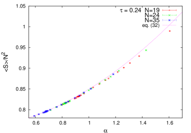
For all values of $\tau<2/9$ we observed that there is a discontinuity in the expectation value of the action $<S>$ across the transition line in Figure 3. This jump in ${\cal S}$ is well predicted by the theoretical expression

$$\Delta{\cal S}=-\tilde{\alpha}^{4}(-\frac{\tau\phi^{2}_{*}}{8}+\frac{\phi^{3}_{*}}{24})$$ (34)

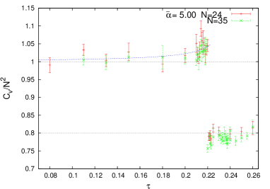
with $\phi_{*}$ given by equation (9) evaluated on the transition. The specific heat is non-analytic along the transition, but the nature of its non-analyticity differs on the critical line $\tau=\frac{2}{9}$ and the critical curve $(\tau<\frac{2}{9},\tilde{\alpha}_{*}(\tau))$. In the former case the specific heat has the standard jump of a 1st order transition while on the latter it diverges as the transition is approached from the low temperature or fuzzy sphere phase side of the transition but there is no observable increase in the specific heat as the transition is approached from the high temperature side.

To identify the transition we choose that value of $\tilde{\alpha}$ that gives the specific heat and identify this as $\tilde{\alpha}_{*}$. In figure 5 we show the curve of the specific heat $C_{v}$ for fixed values of $\tau=0.08$ and $\tau=0.15$. The critical value of the coupling $\tilde{\alpha}_{*}$ measured from simulation is $2.40\pm 0.05$ for $\tau=0.08$ whereas we found a value of $\tilde{\alpha}_{*}=2.85\pm 0.05$ when $\tau=0.15$. These are to be compared to the prediction (12) from which we get the values $\tilde{\alpha}_{*}=2.366$ and $\tilde{\alpha}_{*}=2.790$ respectively. As we can see the numerical results are in good agreement with the our theoretical predictions.

Thought the transition is characterised by a latent heat, as it was pointed out in [19, 20], it is unusual in that there are also critical fluctuations in the specific heat as the transition is approached from the low temperature phase for $\tau<\frac{2}{9}$. These lead to a divergent specific heat with specific heat exponent $\alpha=1/2$. Our simulations are consistent with the expected divergence in the low temperature phase.

In figure 6, where we show ${\cal S}$ for $\tau=1/4$ and $\tilde{\alpha}<3.7$. We see the data collapses when plotted against $\alpha$. We also show that the specific heat is fluctuating around $C_{v}=\frac{3}{4}$. These are consistent with a uniform distribution of commuting $X_{a}$ whose eigenvalues are distributed within a ball of radius $R=2.0$.

In figure 7, we show ${\cal S}$ and the specific heat as a function of $\tau$ for $\tilde{\alpha}=5.0$ and we observe that the transition occurs at $\tau=0.219\pm 0.005$ a value consistent with $\tau=\frac{2}{9}$. We have chosen $\tilde{\alpha}=5.0$ to represent the typical behaviour for $\tilde{\alpha}>\tilde{\alpha}_{*}(\tau=2/9)=4.02$, so that the curve crosses the critical line $\tau_{*}=2/9$. Our theoretical prediction for the critical value of the specific heat when the transition is approached from the low temperature phase, eq. (22) predicts $C_{v}(\tau=2/9,\tilde{\alpha}=5)=1.02$, which is in agreement with our simulations. Figure 7 also shows that ${\cal S}$ has a bend but there is no apparent, jump. It also appears that the bend occurs at a slightly larger value than $\tau=\frac{2}{9}$. The precision of our numerical results show that the bend occurs at $\tau=0.222\pm 0.002$, showing small deviations when $\tilde{\alpha}$ is close (and larger) to $\tilde{\alpha}_{*}(\tau=2/9)=4.02$ where the transitions take place at slightly larger values than $\tau=\frac{2}{9}$ (see figure 3), however this might be due to finite size effects. The specific heat shows there are no strong fluctuations, so the classical theory should be a good approximation and in fact predicts the critical point $\tau_{*}=2/9$ see eq. (12). The finite size effects in the specific heat are consistent (31) and account for the deviation from the limiting large $N$ value of $C_{v}=0.75$.

4.1 Eigenvalue distributions

By measuring the eigenvalue distribution of the matrices $X_{a}$ and the commutators $i[X_{a},X_{b}]$ we can investigate in more detail the features of the configurations at quantum level. The model has global $SO(3)$ invariance, therefore each of the three matrices has the same eigenvalue distribution and also each of the commutators share a common distribution. We also measure the eigenvalues for the $2N\times 2N$ matrix

$${\mathbb{C}}=\sigma_{a}X_{a}$$ (35)

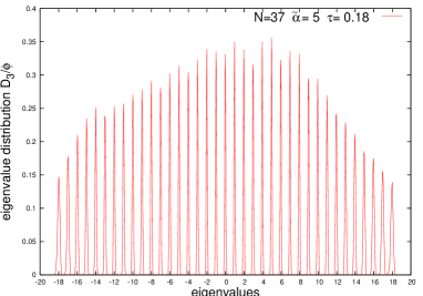
where $\sigma_{a}$ are the three Pauli matrices. This matrix is particularly useful because it encodes information from the three matrices $X_{a}$ simultaneously and its spectrum can be easily computed for specific configurations. For instance, when $X_{a}=\alpha L_{a}$, where $L_{a}$ are IRRs of $SU(2)$, with $L_{a}L_{a}=\frac{N^{2}-1}{4}$, we have

$$(\sigma_{a}L_{a})^{2} = L^{2}_{a}-\sigma_{a}L_{a}\;\;\;\mbox{then}\qquad(\sigma_{a}L_{a}+\frac{1}{2})^{2}=\frac{N^{2}}{4}\mathbf{1}$$ (36)

and we find that with ${\mathbb{C}}\to U^{-1}{\mathbb{C}}_{diag}U$ with $U\in U(2N)$ and noting that ${\mathbb{C}}$ is traceless and is the $SU(2)$ tensor product $2\otimes N=(N+1)\oplus(N-1)$ we see that the eigenvalue multiplicities are $N-1$ for $-\frac{N}{2}-\frac{1}{2}$ and $N+1$ for $\frac{N}{2}-\frac{1}{2}$ therefore

$${\mathbb{C}}_{diag}=\alpha\left(\frac{(N-1)}{2}\mathbf{1}_{N+1}\oplus\frac{(-N-1)}{2}\mathbf{1}_{N-1}\right).$$ (37)

More generally for a reducible representation $J_{a}$ of (5) we have

$${\mathbb{C}}_{diag}=\alpha\oplus_{i}\left(\frac{(n_{i}-1)}{2}\mathbf{1}_{n_{i}+1}\oplus\frac{(-n_{i}-1)}{2}\mathbf{1}_{n_{i}-1}+{\bf 0}\right).$$ (38)

where ${\bf 0}$ corresponds to the one dimensional representations in $J_{a}$. We see that ${\mathbb{C}}$ is sensitive to the representation content of the matrices. The spectrum of ${\mathbb{C}}$ will have distinct eigenvalues for the different $SU(2)$ IRRs present in $X_{a}$.

We also measure the eigenvalues of the Dirac operator

$$\mathbb{D}:=\sigma_{a}[X_{a},\;\cdot],$$ (39)

where $[X_{a},\cdot]$ means $X_{a}$ acting as commutator: $[X_{a},M]=X_{a}M-MX_{a}$ for any matrix $M\in Mat_{N}$.

The spectrum of $\mathbb{D}=\sigma_{a}[X_{a},\cdot]$ can be easily computed when $X_{a}=\alpha L_{a}$. For this particular case we have

$$\mathbb{D}=\sigma_{a}[X_{a},\;\cdot]=\alpha\;\sigma\cdot\mathcal{L}=\alpha\left[{\cal J}_{a}^{2}-{\cal L}_{a}^{2}-\frac{3}{4}\right]=\alpha\left[j(j+1)-l(l+1)-\frac{3}{4}\right],$$ (40)

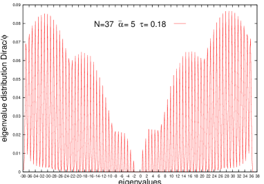
with $j=l\pm\frac{1}{2}$ with $l$ taking the values $l=0,1,..,N-1$ and we obtain the spectrum

$$spec\{\mathbb{D}\} = \alpha\left\{\begin{array}[]{rcl}l;&j=l+\frac{1}{2},&g(l)=2(l+1)\\ -(l+1);&j=l+\frac{1}{2},&g(l)=2l\\ 0;&l=0,&g(l)=2\end{array}\right.$$ (44)

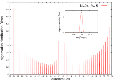
$g(l)$ is the degeneracy. The Dirac operator $\mathbb{D}$ has therefore the spectrum

$$spec\{\mathbb{D}\}=\alpha\{-N,-(N-1),\dots,-3,-2,0,1,2,3,\dots,(N-1)\}.$$ (45)

This spectrum is well reproduced in our numerical simulations for the parameter range of the phase diagram Figure 3 corresponding to the fuzzy sphere, see Figure 10.

4.2 Numerical results for eigenvalue distributions

4.2.1 The $\tau=0$ case

We begin with our results for the case $\tau=0$. This situation corresponds to the model studied in [15, 19, 20] and the system crosses the phase boundary of Figure 3 at $\tilde{\alpha}=2.08$ as predicted from the effective potential or $\tilde{\alpha}=2.01\pm 0.01$ as measured from simulations.

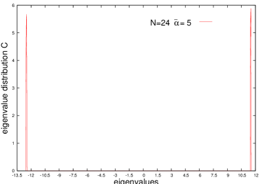
In the low temperature phase (large $\tilde{\alpha}$), the dominant configurations are IRRs of $SU(2)$, $D_{a}\sim L_{a}$. Figure 9 shows the eigenvalue distribution for $N=24$ and $\tilde{\alpha}=5.00$ and $\tau=0$. The simulation indeed shows that the spectrum of both $D_{3}$ and $i[D_{1},D_{2}]$ are discrete and equally spaced consistent with an IRR of $SU(2)$.

In figure 10, the eigenvalues for the matrix $C=\sigma_{a}D_{a}$ and the Dirac operator ${\cal D}=\sigma_{a}[D_{a},\cdot]$ are shown and are consistent with the spectrum (37) for matrix ${\mathbb{C}}$, and (45) for $\mathbb{D}$.

Figure 9: Eigenvalues for $D_{3}$ and $i[D_{1},D_{2}]$. We observe a discrete spectrum. $N=24$, $\tilde{\alpha}=5.00$, $\tau=0.0$.

Figure 10: Eigenvalues for matrix $C=\sigma_{a}D_{a}$ and Dirac operator ${\cal D}=\sigma_{a}[D_{a},]$. $N=24$, $\tilde{\alpha}=5.00$, $\tau=0.0$. The eigenvalues for the matrix $C$ are nicely distributed in two peaks around $C=-\frac{25}{2}=-12.5$ and $C=+\frac{23}{2}=11.5$ as expected. While the operator ${\cal D}$ reproducing the spectrum (45).

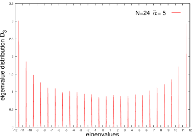
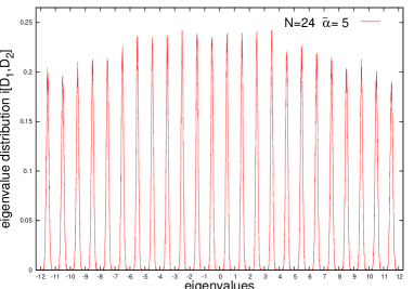
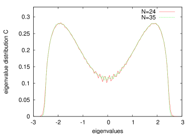
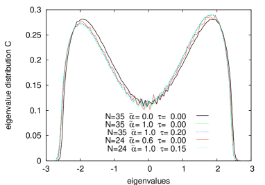
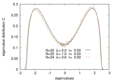
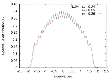
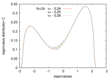
In the matrix phase, we observe a continuous spectrum for the matrices $X_{a}$; we also observe that the eigenvalue distribution for $X_{a}$ has an increasing number of oscillations and becomes a smooth convex spectrum for large $N$ and as might be expected from (23) the spectrum of $X_{a}$ is largely independent of $\tilde{\alpha}$. The eigenvalue distribution of each $X_{a}$ is symmetric around zero and its support is localised within the interval $[-2,2]$ and the parabola law (25) fits excellently with $R=2.0$. The distribution for the commutator is also symmetric around zero.

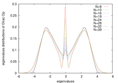
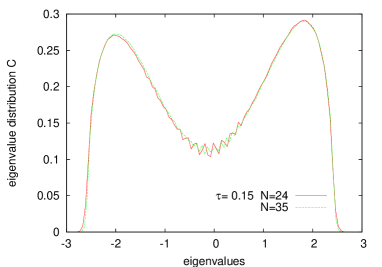
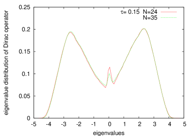
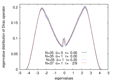
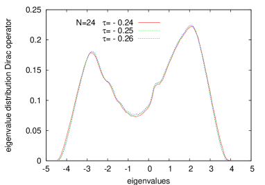
The matrix $\mathbb{C}=\sigma_{a}X_{a}$ shows a distribution with two maxima around $\pm 2$. The distribution, however, is not symmetric with the peak on the right hand slightly higher than the one on the left. There is a small effect of non-zero $\tilde{\alpha}$ which is larger than any effect on $X_{a}$ or $i[X_{a},X_{b}]$. The distribution for the operator $\mathbb{D}$ has three peaks for small $N$, with the central peak around zero disappearing as $N$ is increased. The distribution also shows a slight distortion with the right hand peak larger than the left. Numerical results are shown in figure 11 and 12 for $N=24,35$ with $\tilde{\alpha}=1.00$, in figure 12 we also show the case $N=24$ with $\tilde{\alpha}=0.60$ in order to compare.

Figure 11: Eigenvalues for $X_{3}$ and $i[X_{1},X_{2}]$ in matrix phase. $N=24$, $\tilde{\alpha}=1.00$, $\tau=0.0$.

Figure 12: Eigenvalues for matrix $\mathbb{C}=\sigma_{a}X_{a}$ and Dirac operator $\mathbb{D}=\sigma_{a}[X_{a},]$ in the matrix phase $N=24$, $\tilde{\alpha}=0.60,1.00$, and $N=35$, $\tilde{\alpha}=1.00$ for $\tau=0.0$. The eigenvalue distributions for the matrix $\mathbb{C}$ and operator $\mathbb{D}$ are asymmetric

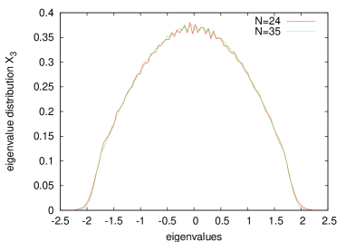
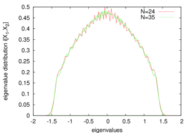
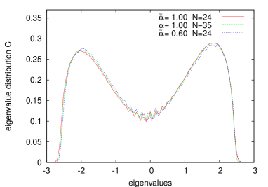
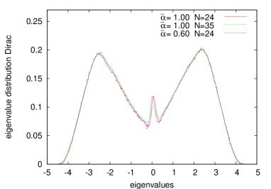
We highlight the special case of both $\tau=\alpha=0$ which we refer to as the pure Yang-Mills matrix model and show the distributions of $X_{a}$, $i[X_{a},X_{b}]$, in figure 13 and those of ${\mathbb{C}}$ and ${\mathbb{D}}$ in figure 14. These are all symmetric and consistent with our interpretation of the matrix phase as fluctuations around commuting matrices whose joint eigenvalue distribution is a solid ball of radius $R=2.0$.

Figure 13: Eigenvalues for $X_{3}$ (left) and $i[X_{1},X_{2}]$ (right) for pure Yang-Mills matrix model for different $N$. The eigenvalue distribution of $X_{3}$ is fit by the parabolic distribution (25) with $R=2.0$ (solid line) and is consistent with a background of commuting matrices whose eigenvalues are uniformly distributed inside a solid 3-ball of radius $R$.

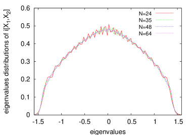
The eigenvalue distribution for $\mathbb{C}=\sigma_{a}X_{a}$ has two peaks at approximately $\pm 1.9$. In the large $N$ limit the Dirac operator $\mathbb{D}$, has two peaks peaks located at approximately $\pm 2.4$ and support of its spectrum lies in the interval $[-4,4]$.

Figure 14: Eigenvalues for matrix $\mathbb{C}=\sigma_{a}X_{a}$ and the Dirac operator $\mathbb{D}=\sigma_{a}[X_{a},]$ for the pure Yang-Mills matrix model. Both distributions are symmetric.

4.2.2 The $\tau\neq 0$ case

We again focus on the eigenvalue distributions of the observables; $D_{a}$, $i[D_{a},D_{b}]$, $C=\sigma_{a}D_{a}$ and the operator Dirac ${\cal D}$ in the fuzzy sphere phase and $X_{a}$, $i[X_{a},X_{b}]$, $\mathbb{C}$ and $\mathbb{D}$ in the matrix phase. By a close inspection of the spectrum of these matrices we confirm that the numerical results are in good accord with $\phi$ as predicted by equation (9) in the fuzzy sphere phase as we will now describe.

Fuzzy sphere phase.

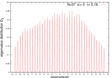
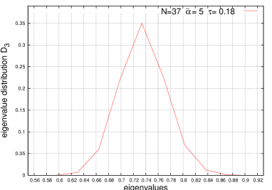
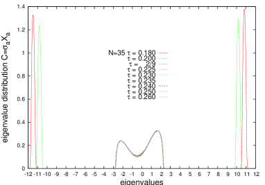
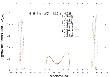
The eigenvalue distributions in the region of the parameter space in which the fuzzy sphere solution $D_{a}=\phi L_{a}$ exists is delimited by the critical line (12) and defined for $\tilde{\alpha}>\tilde{\alpha}_{*}$ whenever $\tau<2/9$. The effect of $\tau$ is to increase the critical point $\tilde{\alpha}_{*}$ according to (12), in other words, the critical temperature at which the transition occurs, is lowered. For a specific set of parameter $N,\tilde{\alpha}$ we can measure the value for $\phi$ for a fixed value $\tau$. Knowing that in this phase the ground state is an IRR of $SU(2)$, i.e. $D\sim\phi\;diag(-s,-(s-1),\cdots,+(s-1),+s)$ (with $s$, the spin labeling the IRR: $s=\frac{N-1}{2}$) we can extract the value of $\phi$ measured in simulations since $\phi=\frac{1}{s}\;\mbox{eigenvalues($D$)}(=\frac{\sqrt{N}}{\tilde{\alpha}s}\;\mbox{eigenvalues($X$)})$. For instance, in Figure 15(a) for $N=37$, $\tilde{\alpha}=5$, $\tau=0.18$ using the largest eigenvalue, the simulation gives $\phi=0.7539$ while the prediction (9) gives $\phi=0.75$.

Selecting the first positive and negative eigenvalues of $D_{a}$, which should correspond to $ev(L_{3})=\pm 1$, we obtain $\mbox{ev}(D_{a})_{1}=0.73$ and $\mbox{ev}(D_{a})_{-1}=-0.77$, (see figure 15(b)). Taking the average modulus we can get an estimate for $\phi$ of $\phi=0.75$ while the predicted value from eq.(9) is $\phi=0.7537$. We can now replot $D_{a}/\phi$ and the operator $\mathbb{D}/\phi$ in figure 16; we can observe that the configurations are indeed around $D_{a}/\phi\sim L_{a}$. Our numerical results are in excellent agreement with the analytical predictions.

Figure 15: (a) Eigenvalues for matrix $D_{a}$ deep inside the fuzzy sphere region $\tilde{\alpha}=5$ and $\tau=0.18$. (b) On the right a zoom for the first peak on the right side of zero eigenvalue of $D_{a}$ from which the value for $\phi$ is measured.

Figure 16: Eigenvalues for matrix $D_{a}$ and the operator $\mathcal{D}=\sigma_{a}[D_{a},\cdot]$ deep inside the fuzzy sphere region $\tilde{\alpha}=5$ and $\tau=0.18$. The eigenvalues are divided by the measured value of $\phi=0.75$ in order to show that $D_{a}/\phi$ are fluctuating around $L_{a}$, irrep. $SU(2)$ for $N=37$.

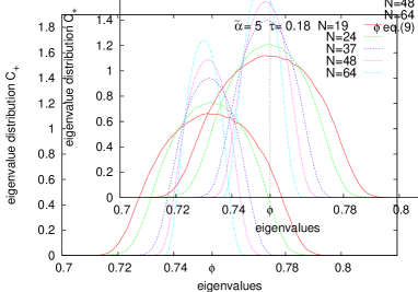
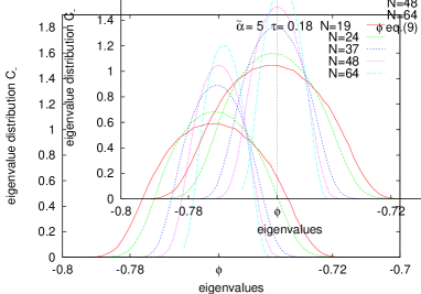
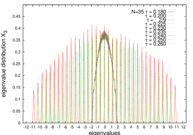
Alternatively, we can extract $\phi$ from the eigenvalue distribution of matrix $C=\sigma_{a}D_{a}$. In the fuzzy sphere we have $D_{a}=\phi L_{a}$. We know that the eigenvalues of $C$ are given by

$$C_{\pm}=\alpha\phi\left(\pm\frac{N}{2}-\frac{1}{2}\right).$$ (46)

Therefore by choosing for instance $C_{+}$ the value for $\phi$ can be extracted from the numerical results for the corresponding set of parameters. We obtain similar result by choosing $C_{-}$. See figure 17.

Figure 17: Here we use the eigenvalue distribution of the matrix $C=\sigma_{a}D_{a}$ in order to extract the value of $\phi$ since $\frac{2\sqrt{N}C_{+}}{\tilde{\alpha}(N-1)}=\phi$. The parameters are given by $\tilde{\alpha}=5$ and $\tau=0.18$, for different values of $N$. We can see that the numerical value for $\phi$ is in very good agreement with the theoretical prediction $\phi=0.7537$ given by eq.(9). On the left the corresponding plot for $C_{-}$, where $\phi$ is given by $\phi=-\frac{2\sqrt{N}C_{-}}{\tilde{\alpha}(N+1)}$.

Figure 18: Eigenvalues for $X_{3}$ and $i[X_{1},X_{2}]$ for different $N$, $\tau=0.15$ in the matrix phase $\tilde{\alpha}=1$. Eigenvalues distribute uniformly inside a 3-solid ball.

Figure 19: (a) Eigenvalues for matrix $\mathbb{C}=\sigma_{a}X_{a}$. (b) $\mathbb{D}=\sigma_{a}[X_{a},]$ in the matrix phase for $\tau=0.15$, $\tilde{\alpha}=1$

Figure 20: Effect of Myers term on the eigenvalues for matrix $\mathbb{C}=\sigma_{a}X_{a}$ (left) and Dirac operator $\mathbb{D}=\sigma_{a}[D_{a},]$ (bottom) in the matrix phase. We can see that the Myers term has a small effect of the distributions, they are no longer symmetric as compared with the pure Yang-Mills (in black thick line).

Figure 21: Evolution for eigenvalues for matrix $X_{3}$ for fixed $\tilde{\alpha}=5$ for different values of $\tau$. At $\tau=2/9$ the fuzzy sphere disappears. On the right eigenvalues for the matrix $\mathbb{C}=\sigma_{a}X_{a}$.

Figure 22: The spectrum of ${\mathbb{C}}=\sigma_{a}X_{a}$ for varying $\tau$ at $\tilde{\alpha}(\tau=2/9)=4.02$. We see that the transition occurs at $\tau=0.213\pm 0.002$.

Figure 23: The eigenvalue distributions for $X_{3}$, $\mathbb{C}$ and ${\mathbb{D}}$ for $\tilde{\alpha}=5.0$ and $\tau>2/9$. We also show the thermalisation history for $N=24$ and $\tilde{\alpha}=5.0$ with $\tau=0.24$, for different initial conditions, $D_{a}=0$ (Z), random start (R) and fuzzy sphere start $D_{a}=L_{a}$ (L).

Figure 24: Effect of the mass term $\frac{r}{2}TrX^{2}_{a}$ in the Yang-Mills action. Fixing $\frac{r}{2}=0.20$ for different values of $N$ we plot the eigenvalues for matrix $X_{a}$ (left) and $\mathbb{C}=\sigma_{a}X_{a}$ (right). We compare with the $r=0$ ($\tau=0$) case. The eigenvalue distribution for the configurations $X_{a}$ is fit by the parabola (25) as in the pure Yang-Mills model (thick line). We conclude that the mass term has no effect in the Yang-Mills matrix action.

Matrix phase.

In this phase as we have mentioned before, the dependence on $N$ drops out if we concentrate on $X_{a}=\alpha D_{a}=\frac{\tilde{\alpha}}{\sqrt{N}}D_{a}$ as our basic operator. We observe that the distribution for eigenvalues coincides, to our numerical accuracy, with that of the pure Yang-Mills model and there is no observable dependence on the parameters $\alpha$, $\tau$ and matrix size $N$. The data is well fit by the parabolic distribution (25) with $R=2.0$. We also observe that the eigenvalue distribution of the commutator shows no observable deviation from that of the pure Yang-Mills model. Figure 18 shows the case for $\tau=0.15$, $\tilde{\alpha}=1$ for different matrix size.

In our simulations we observe that the spectrum of the matrix $\mathbb{C}=\sigma_{a}X_{a}$ and the operator ${\mathbb{D}}$ are not symmetric, but rather distorted with respect to the pure Yang-Mills case; see figure 19(a) for $\tau=0.15$ and fixed value $\tilde{\alpha}=1$ and figure 20 (a) and (b) for ${\mathbb{C}}$ and figure 20 (c) for ${\mathbb{D}}$. As we see from the graphs the asymmetry is due to the Myers term. We attribute this asymmetry to a residual dependence on the Myers term which drops out as $\frac{1}{\sqrt{N}}$, noting that graphs correspond to $\alpha=0,0.122$ and $\alpha=0.169$ for $\tilde{\alpha}=0,0.6$ and $\tilde{\alpha}=1.0$ respectively.

The operator $\mathbb{D}$ has a continuous spectrum and turning on the Meyrs term again gives an observable asymmetry to its spectrum, see figure 19(b) for $\tilde{\alpha}=1.0$ and fixed value $\tau=0.15$ and figure 20 (c) for a range of parameter values. It is only for $\tau\geq\frac{2}{9}$ that the asymmetry survives the large $N$ limit since for all $\tau<\frac{2}{9}$ increasing $N$ for fixed $\alpha$ drives across the transition line and into the fuzzy sphere phase.

From the distributions we can see that the transitions that takes place in the model is the one which goes from a non-commutative fuzzy sphere as geometrical background to a solid 3-ball with fixed radius $R=2$.

$$X_{a}^{2}=\frac{N^{2}-1}{4}\alpha^{2}\phi^{2}\;\;\;\longrightarrow\;\;\;X_{a}^{2}\leq 4$$ (47)

Or if we rescale to the $D_{a}$ we get a collapse of a sphere to a point.

This transition occurs when $\tilde{\alpha}$ reaches the critical value $\tilde{\alpha}_{*}$ following the critical in the phase diagram depicted in figure 3. The transition line is defined by the critical curve (12) whenever $\tau$ is in the range $0\leq\tau<2/9$. The model is unstable for $\tau<0$. However, when $\tau<0$ and $\tilde{\alpha}>\tilde{\alpha}_{*}(\tau)$, the fuzzy sphere is a local minimum of the model with negative action which goes to $-\infty$ as $N\rightarrow\infty$ and tunneling out of this well becomes impossible.

In figure 21 we track the evolution of the eigenvalue distribution of $X_{a}$ and matrix ${\mathbb{C}}$ as a function of $\tau$ along the line $\tilde{\alpha}=5.0$ starting in fuzzy sphere. We can see the fuzzy sphere disappears as we cross the critical value $\tau=2/9$. We observe that $\tau=\frac{2}{9}$ actually falls in the matrix phase. We find that the transition tracks the line $\tau=\frac{2}{9}$ for different $\tilde{\alpha}$. However, as the end point of this line is approached, i.e. $\tilde{\alpha}=12\left(\frac{4}{107+51\sqrt{17}}\right)^{1/4}\sim 4.02$ we observe that in a small neighbourhood of this value the transition actually occurs at $\tau_{*}<\frac{2}{9}$ see figure 3. In figure 22 we see that there appears to be some deviation from the predictions of (9) where one would expect that for $\tilde{\alpha}=4.02$ the transition would occur at $\tau=\frac{2}{9}\sim 0.222$, however we find the transition at $\tau=0.213\pm 0.002$. For this transition $<S>$ shows a clear discontinuity consistent with the predictions from (9) and we expect there is still a divergent specific heat though this is more difficult to detect.

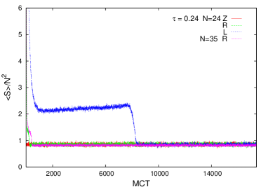
Figure 23 shows the history of the expectation value of the action $<S>/N^{2}$ for $N=24,35$, $\tilde{\alpha}$ and $\tau=0.24$ from different initial configurations; cold ($D_{a}=L_{a}$), zero and random start. When starting from cold configuration we observe the system goes through metastable states. All reach the same energy level and no decay was observed after $2^{19}$ Monte Carlo steps or sweeps, defined as the step in which all the matrix elements are updated according to the Metropolis algorithm.

Massive Yang-Mills model

Since, in the model (23) the limit $\alpha=0$ removes the quadratic and Meyrs term we treat this the massive deformation of this case separately.

For $\alpha=0$ we therefore also study the model

$$S[X]=N\;Tr\left(-\frac{1}{4}[X_{b},X_{b}]^{2}+\frac{r}{2}X^{2}_{a}\right).$$ (48)

We study the eigenvalue distributions for matrix $X_{a}$ and matrix $\mathbb{C}=\sigma_{a}X_{a}$ for different values of the parameter $r$ and matrix size $N$. We find that the phenomenology for this model is similar to that of $\tau=0$ described above. The eigenvalue distribution for the matrix configurations $X_{a}$ and small $r$ are fit by the parabola (25).

We also observe that the eigenvalues for the matrix $\mathbb{C}$ distribute as in the pure Yang-Mills model. See figure 24. For values $\frac{r}{2}<0$ the matrix action is not bounded from below.

Comment on the Massive Myers model with complex Meyrs coupling.

For completeness let us consider the following action

$$S=N\;\mbox{Tr}\;\left(\frac{i\alpha}{3}\epsilon_{abc}X_{a}[X_{b},X_{b}]+\frac{r}{2}X^{2}_{a}\right).$$ (49)

The model is exactly solvable (see Hoppe [24]) and is equivalent to a 2-matrix Yang-Mills model with massive deformation. For real $\alpha$ the model is not stable with no ground state. It may however be possible to localise configurations in a well by suppressing tunneling in the large $N$ limit. We observe that such wells exist for large positive $r$.

5 Conclusions

We have performed numerical simulations of a simple two parameter 3-matrix model with energy functional given by (2). In particular we studied the phase diagram as a function of the two parameters $\tau$ and $\tilde{\alpha}$. Earlier studies [20] looked at the case $\tau=0$ and found that it exhibited an exotic phase transition at $\tilde{\alpha}_{*}={(\frac{8}{3})}^{3/4}$. It was argued, based on an effective potential calculation that the model should have a line of phase transitions dividing the $(\tau,\tilde{\alpha})$ plane in two and predicting the coexistence curve. We find that for $0<\tau<\frac{2}{9}$ the coexistence curve is predicted well by the theoretical expressions. The coexistence curve asymptotes to the line $\tau=\frac{2}{9}$ and appears to deviate slightly from the prediction of the effective potential (9). This special value of $\tau$ corresponds to the value where the action is a complete square, see eq. (6). We examine the eigenvalue distributions of different operators. In particular we look at $\mathbb{C}=\sigma_{a}X_{a}$ which detects the $SU(2)$ representation content of the configurations $X_{a}$. We find the IRR of dimension $N$ has fluctuations around a lower $S$ than any other configuration in the parameter range corresponding to the fuzzy sphere phase. Also, in this range the spectrum of ${\mathbb{C}}$ has the two peaks corresponding to $\alpha\phi\sigma_{a}L_{a}$ with $L_{a}$ the $SU(2)$ IRR of dimension $N$. In the parameter range corresponding to the matrix phase ${\mathbb{C}}$ has a continuum spectrum. We also study the Dirac operator $\mathbb{D}=\sigma_{a}[X_{a},\cdot]$ and find that in the fuzzy sphere phase its spectrum is (as expected) a shifted, cutoff version of the commutative sphere.

We found evidence for two distinct transition types in the emergent geometry scenario. For $0<\tau<\frac{2}{9}$ we found that, as the transition is approached from the fuzzy sphere phase with fixed $\tau$, the model has a divergent specific heat with critical exponent $\alpha=\frac{1}{2}$. However for $\tilde{\alpha}>\tilde{\alpha}_{*}=12\left(\frac{4}{107+51\sqrt{17}}\right)^{1/4}\sim 4.02$, and crossing the transition at fixed $\tilde{\alpha}$, there appear to be no critical fluctuations; the transition is one with a continuous, but non-differentiable internal energy, and a discontinuous specific heat. In all cases the transition is from a fuzzy sphere to a matrix phase. We study the matrix phase in detail and find that a useful description of this phase is in terms of fluctuations about a background of commuting matrices whose eigenvalues are concentrated within a sphere of radius $R=2.0$. This is consistent with the estimates of [6] who performed a 2-loop analysis and estimated $R\sim 1.8$

We find that, though it is possible for configurations other than the irreducible fuzzy sphere to be present in the model, they never correspond to the true ground state of the system. Such configurations, were they present, would be easily detected by the matrix ${\mathbb{C}}$. Furthermore for $\tau=\frac{2}{9}$ we find that $<S>$ when trapped in a fuzzy sphere configuration is larger than that for fluctuations in the matrix phase, and the fuzzy sphere is not a true ground state of the system. Also, for $\tau>\frac{2}{9}$ we observe decays from the fuzzy sphere to the matrix phase, i.e. the fuzzy sphere is a meta-stable configuration for the system, with observable decay. In contrast for the critical line $\tau=\frac{2}{9}$ we observe no decay of the fuzzy sphere to the true ground state. We infer that the barrier is sufficiently high in this case that the limit of $N\rightarrow\infty$ prevents tunneling out of the local minimum corresponding to the fuzzy sphere.

A natural further stage in the study undertaken here is to include the effect of Fermions. However, the most interesting case involves either complex actions or fluctuating signs in the Fermionic sector [35] both of which lead to significant numerical difficulties.

In $d=10$ the pure Yang-Mills model has received significant attention in a scenario of emergent gravity [30]. It appears from our study, that for finite $N$, all such configurations will be meta stable. In the large $N$ limit tunneling will be suppressed and these states may become stable. unfortunately, reliable numerical simulations in such a situation are more difficult.

Acknowledgements

R.D.B. was supported by a Marie-Curie Fellowship from the Commission of the European Communities. Currently he acknowledges support from Conacyt Mexico. D.O’C. thanks the Perimeter Institute for hospitality where part of this work was performed.

References

- [1] T.Banks, W.Fischler, S.Shenker and L.Susskind, “M theory as a matrix model: a conjecture”, Phys.Rev. D55:5112 (1997), [hep-th/9610043].
- [2] N.Ishibashi, H.Kawai, Y.Kitazawa, A.Tsuchiya, “A Large N reduced model as superstring”, Nucl.Phys.B 498:467-491( 1997), [hep-th/9612115].
- [3] D. Berenstein, J. Maldacena, H. Nastase, “Strings in flat space and pp waves from Super Yang Mills” JHEP 0204:013 (2002), [hep-th/0202021].
- [4] T.Hotta, J.Nishimura, A.Tsuchiya, “Dynamical Aspects of Large N Reduced Models”, Nucl.Phys. B545:543-575 (1999), [hep-th/9811220].
- [5] Denjoe O’Connor, “Low-dimensional Yang-Mills Theories: Matrix Models and Emergent Geometry”, Theoretical and Mathematical Physics, 169: (2011) 1405-1412.
- [6] V. Filev and D. O’Connor, in preparation.
- [7] H.Grosse, C.Klimčik, P.Prešnajder, “Towards Finite Quantum Field Theory in Non-Commutative Geometry”, Int.J.Theor.Phys. 35:231 (1996), [hep-th/9505175]. “Field Theory on a Supersymmetric Lattice”, Comm.Math.Phys. 185:155 (1997) [hep-th/9507074]. “Topologically nontrivial field configurations in noncommutative geometry” Comm.Math.Phys. 178:507 (1996), [hep-th/9510083].
- [8] U.Carow-Watamura and S.Watamura, “Noncommutative Geometry and Gauge Theory on Fuzzy Sphere”, Comm.Math.Phys. 212:395 (2000), [hep-th/9801195].
- [9] A.P.Balachandran, X.Martin,D.O’Connor “Fuzzy actions and their continuum limits” Int.J.Mod.Phys. A16:2577-2594 (2001), [hep-th/0007030].
- [10] C.S.Chu, J.Madore, H.Steinacker, “Scaling limits of the fuzzy sphere at one loop”, JHEP 0108:038 (2001), [hep-th/0106205].
- [11] B.P.Dolan, D.O’Connor, P.Prešnajder, “Matrix models on the fuzzy sphere”, [hep-th/0204219]. “Matrix models on the fuzzy sphere and their continuum limits”, JHEP 0203:013 (2002), [hep-th/0109084].
- [12] D.O’Connor, “Field theory on low dimensional fuzzy spaces”, Mod.Phys.Lett. A18:2423 (2003).
- [13] H. Steinacker, “Quantized gauge theory on the fuzzy sphere as random matrix model” Nucl.Phys.B 679:66-98 (2004), [hep-th/0307075].
- [14] S.S.Gubser, S.L.Sondhi, “Phase structure of noncommutative scalar field theories”, Nucl.Phys.B605:395-424 (2001) [hep-th/0006119]. J.Ambjorn, S. Catterall, “Stripes From (Noncommutative) Stars”, Phys.Lett. B549:253-259 (2002), [hep-lat/0209106]. W.Bietenholz, F.Hofheinz, J.Nishimura, “Phase diagram and dispersion relation of the noncommutative lambda model in ”. JHEP 0406:042 (2004), [hep-th/0404020].
- [15] T.Azuma, S.Bal, K.Nagao, J.Nishimura, “Nonperturbative studies of fuzzy spheres in a matrix model with the Chern-Simons term” JHEP 0405:005 (2004), [hep-th/0401038].
- [16] X.Martin, JHEP 04 (2004) 077, [hep-th/0402230]; X.Martin, Mod.Phys.Lett.A 18 (2003) 2389-2396.
- [17] D.O’Connor, B.Ydri, “Monte Carlo Simulation of a NC Gauge Theory on The Fuzzy Sphere”, JHEP 0611:016 (2006), [hep-lat/0606013].
- [18] M.Panero, “Quantum field theory in a non-commutative space: Theoretical predictions and numerical results on the fuzzy sphere”, SIGMA 2:081 (2006), [hep-th/0609205]. “ Numerical simulations of a non-commutative theory: The Scalar model on the fuzzy sphere”, JHEP 0705:082 (2007), [hep-th/0608202].
- [19] R.Delgadillo-Blando, D.O’Connor, B.Ydri, “Geometry in transition: A model of emergent geometry”, Phys.Rev.Lett. 100:201601, [arXiv:0712:3011] .
- [20] R.Delgadillo-Blando, D.O’Connor, B.Ydri, “Matrix models, emergent geometry and gauge theory”, JHEP 0509:049 (2009), arXiv:08060558 [hep-th].
- [21] T.Azuma, S.Bal, J.Nishimura, “Dynamical generation of gauge groups in the massive Yang-Mills-Chern-Simons matrix model”, PRD72 (2005), [hep-th/0504217].
- [22] R.Myers, “Dielectric branes”, JHEP 9912:022 (1999), [hep-th/9910053].
- [23] J. Madore, “The Fuzzy sphere”, Class. Quantum. Grav. 9:69-88 (1992).
- [24] J.Hoppe, “Quantum Theory of A Massless Relativistic Surface and A Two-Dimensional Bound State Problem” MIT Ph.D.Thesis, 1982.
- [25] P.Castro-Villarreal, R.Delgadillo-Blando, B.Ydri, “A gauge invariant UV-IR mixing and the corresponding phase transition for fields on fuzzy sphere”, Nucl.Phys. B704:111-153 (2005)[hep-th/0405201].
- [26] P.Castro-Villarreal, Rodrigo Delgadillo-Blando ,B.Ydri , “ Quantum effective potential for fields on ”, JHEP 0509:066 (2005), [hep-th/0506044].
- [27] “Towards Noncommutative Fuzzy QED”, R.Delgadillo-Blando, Badis Ydri, JHEP 0703:056 (2007), [hep-th/0611177]. P.Castro-Villarreal, Rodrigo Delgadillo-Blando ,B.Ydri , “ Quantum effective potential for fields on ”, JHEP 0509:066 (2005), [hep-th/0506044].
- [28] D.Dou, B.Ydri “Topology change from quantum instability of gauge theory on fuzzy ”, Nucl.Phys.B 771:167-189 (2007), [hep-th/0701160].
- [29] W.Krauth, M.Staudacher, “Finite Yang-Mills integrals” Phys.Lett. B430:350 (1998), [hep-th/9804199]
- [30] H.Steinacker, “Emergent Gravity from Noncommutative Gauge Theory”, JHEP 0712:049 (2007), arXiv:0708.2426 [hep-th], H. Steinacker, “Emergent Gravity from Noncommutative Gauge Theory” JHEP 0712:049 (2007), [arXiv:0708.2426] [hep-th]. “Emergent 4D gravity from matrix models”, arXiv:0712.3194 [hep-th]. H.Grosse, H.Steinacker, M.Wohlgenannt, “ Emergent Gravity, Matrix Models and UV/IR Mixing”, arXiv:0802.0973 [hep-th],“Emergent Geometry and Gravity from Matrix Models: an Introduction”,Class.Quant.Grav. 27:133001 (2010),arXiv:1003.4134 [hep-th], “Non-commutative geometry and matrix models”, H.Steinacker, arXiv:1109.5521 [hep-th],
- [31] A.Connes, “Noncommutative Geometry”, Academic Press, London,1994. Landi, “An introduction to noncommutative spaces and their geometry”, springer (1997). J.M. Gracia-Bondia, J. C. Varilly, H. Figueroa, “Elements of Noncommutative Geometry”, Birkhauser (2000). J.Madore, “An Introduction to Noncommutative Differential Geometry and its Physical Applications”, Cambridge Press (1995).
- [32] V.A. Kazakov, I.K. Kostov, N.A. Nekrasov, “D-particles, matrix integrals and KP hierarchy”, Nucl.Phys. B557 (1999) 413-442, [hep-th/9810035].
- [33] A.P.Balachandran, “Quantum space-times in the year 2002”, Pramana 59:359-368 (2002) [hep-th/0203259].
- [34] A.P. Balachandran, S. Kurkcuoglu, S. Vaidya “Lectures on fuzzy and fuzzy SUSY physics”, Singapore: World Scientific (2007) 191 p. [hep-th/0511114].
- [35] K.N.Anagnostopoulos, T.Azuma, J.Nishimura, “A general approach to the sign problem - the factorization method with multiple observables”. arXiv:1009.4504 [cond-mat.stat-mech]