11institutetext: Graduate University of Chinese Academy of Sciences, Beijing, China 22institutetext: State Key Lab. of Comput. Sci., Institute of Software, CAS, Beijing, China
33institutetext: Dept. of Comput. Sci., University of New Mexico, Albuquerque, NM, USA
44institutetext: CISS, CS, Aalborg University, Denmark

A “Hybrid” Approach for Synthesizing Optimal Controllers of Hybrid Systems: A Case Study of the Oil Pump Industrial Example

Hengjun Zhao 1122    Naijun Zhan 22    Deepak Kapur 33    Kim G. Larsen 44
Abstract

In this paper, we propose an approach to reduce the optimal controller synthesis problem of hybrid systems to quantifier elimination; furthermore, we also show how to combine quantifier elimination with numerical computation in order to make it more scalable but at the same time, keep arising errors due to discretization manageable and within bounds. A major advantage of our approach is not only that it avoids errors due to numerical computation, but it also gives a better optimal controller. In order to illustrate our approach, we use the real industrial example of an oil pump provided by the German company HYDAC within the European project Quasimodo as a case study throughout this paper, and show that our method improves (up to 7.5%percent7.57.5\%) the results reported in [3] based on game theory and model checking.

Keywords:
Hybrid System, Optimal Control, Quantifier Elimination, Numerical Computation

1 Introduction

Hybrid systems such as physical devices controlled by computer software, are systems that exhibit both continuous and discrete behaviors. Controller synthesis for hybrid systems is an important area of research in both academia and industry. A synthesis problem focuses on designing a controller that ensures the given system will satisfy a safety requirement, a liveness requirement (e.g. reachability to a given set of states), or meet an optimality criterion, or a desired combination of these requirements.

Numerous work have been done on controller synthesis for safety and/or reachability requirements. For example, in [1, 27], a general framework for synthesizing controllers based on hybrid automata to meet a given safety requirement was proposed, which relies on backward reachable set computation and fixed point iteration; while in [24], a symbolic approach based on templates and constraint solving to the same problem was proposed, and in [25], the symbolic approach is extended to meet both safety and reachability requirements.

However, the optimal controller synthesis problem is more involved, also quite important in the design of hybrid systems. In the literature, few work has been done on the problem. Larsen et al proposed an approach based on energy automata and model-checking [3], while Jha, Seshia and Tiwari gave a solution to the problem using unconstrained numerical optimization and machine learning [14]. However, in [3], allowing control only to be exercised at discrete points in time certainly limits the opportunity of synthesizing the optimal controller (though one can get arbitrarily close). Moreover, discretizing could cause an incorrect controller to be synthesized — which therefore requires a posterior analysis (e.g. in [3], PHAVER [9] is used for the purpose). The approach of [14] suffers from imprecision caused by numerical computation, and cannot synthesize a really optimal controller sometimes because the machine learning technique cannot guarantee its completeness.

In this paper, we propose a “hybrid” approach for synthesizing optimal controllers of hybrid systems subject to safety requirements. The basic idea is as follows. Firstly, we reduce optimal controller synthesis subject to safety requirements to quantifier elimination (QE for short). Secondly, in order to make our approach scalable, we discuss how to combine QE with numerical computation, but at the same time, keep arising errors due to discretization manageable and within bounds. A major advantage of our approach is not only that it avoids errors due to numerical computation, but it also gives a better optimal controller.

Application of QE in controller synthesis of hybrid systems is not new. The tool HyTech was the first symbolic model checker that can do parametric analysis [12] for linear hybrid automata, but for the oil pump example it will abort soon due to arithmetic overflow errors. Recently, verification and synthesis of switched dynamical systems using QE were discussed in [23], where the authors gave principles and heuristics for combining different tools, to solve QE problems that are out of the scope of each component tool.

Our encoding of a MIN-MAX-MIN optimization problem into a QE problem is inspired by the idea in [7]: minimizing an objective function f(x1,x2,,xn)𝑓subscript𝑥1subscript𝑥2subscript𝑥𝑛f(x_{1},x_{2},\ldots,x_{n}) can be solved by introducing an additional constraint zf(x1,x2,,xn)𝑧𝑓subscript𝑥1subscript𝑥2subscript𝑥𝑛z\geq f(x_{1},x_{2},\ldots,x_{n}) and eliminating variables x1,x2,,xnsubscript𝑥1subscript𝑥2subscript𝑥𝑛x_{1},x_{2},\ldots,x_{n}, where z𝑧z is a newly introduced variable. Similar ideas can also be found in [4].

The computation of optimal control strategies in this paper is typically a parametric optimization problem, a topic researched extensively in both operation research and control communities. Symbolic methods have advantages in addressing parametric optimization problems [28, 8, 15]. However, we do not find any algorithm suitable for solving a parametric quadratic optimization problem over constraint with complex Boolean structure and hundreds of (or thousands of) atomic formulas as in this paper.

It was shown in [2] that for certain parametric quadratic optimization problems, the closed form solution exists: the optimizer is a piecewise affine function in the parameters, and the optimal value is a piecewise quadratic function in the parameters. Our experiment results confirm this.

In order to illustrate our approach, we use the oil pump industrial example provided by the German company HYDAC within the European project Quasimodo as a case study throughout this paper, and show that our method results in a better optimal controller (up to 7.5%percent7.57.5\% improvement) than those reported in [3] based on game theory and model checking. Moreover, we prove that the theoretically optimal controller of the oil pump example can be synthesized and its correctness is also guaranteed with our approach.

1.0.1 Paper Organization:

In Section 2 we propose a general framework for optimal controller synthesis of hybrid systems based on quantifier elimination and numerical computation. We focus on the oil pump case study in Section 3-6: a description of the oil pump control problem is given in Section 3, modeling of the system and safety requirements is shown in Section 4, a “hybrid” approach for performing optimization is presented in Section 5, and further improvement through a modification in the model is discussed in Section 6. We finally conclude this paper by Section 7.

2 The Overall Approach

In this section we propose an approach that reduces optimal controller synthesis of hybrid systems subject to safety requirements to QE. Such reduction is based on reachable set computation or approximation of hybrid systems and symbolic optimization. We also discuss how numerical computation can be incorporated into our approach to make it more scalable.

Generally, a hybrid system consists of a set of continuous state variables 𝐱𝐱\mathbf{x} (ranging over nsuperscript𝑛\mathbb{R}^{n}) and a set of discrete operating modes Q𝑄Q, with each of which a continuous dynamics is associated specifying the behavior of 𝐱𝐱\mathbf{x} at each mode; discrete jumps between different modes may happen if some transition conditions are satisfied by 𝐱𝐱\mathbf{x}.

The optimal controller synthesis problem studied in this paper can be stated as follows. Suppose we are given an under-specified hybrid system \mathcal{H}, in which the transition conditions are not determined but parameterized by 𝐮𝐮\mathbf{u}, a vector of control parameters. Our task is to determine values of 𝐮𝐮\mathbf{u} such that \mathcal{H} can make discrete jumps at desired points, thus guaranteeing that

  • 1)

    a safety requirement 𝒮𝒮\mathcal{S} is satisfied, that is, 𝐱𝐱\mathbf{x} stays in a designated safe region at any time point; and

  • 2)

    an optimization goal 𝒢𝒢\mathcal{G}, possibly

    min𝐮g(𝐮),max𝐮2min𝐮1g(𝐮),ormin𝐮3max𝐮2min𝐮1g(𝐮),subscript𝐮𝑔𝐮subscriptsubscript𝐮2subscriptsubscript𝐮1𝑔𝐮orsubscriptsubscript𝐮3subscriptsubscript𝐮2subscriptsubscript𝐮1𝑔𝐮\min_{\mathbf{u}}g(\mathbf{u}),\,\,\max_{\mathbf{u}_{2}}\min_{\mathbf{u}_{1}}g(\mathbf{u})\,,\,\mathrm{or}\,\,\min_{\mathbf{u}_{3}}\max_{\mathbf{u}_{2}}\min_{\mathbf{u}_{1}}g(\mathbf{u})\,,

    where g(𝐮)𝑔𝐮g(\mathbf{u}) is an objective function in parameters 𝐮𝐮\mathbf{u}, is achieved.

Then our approach for solving the synthesis problem can be described as the following steps.

2.0.1 Step 1.

Derive constraint D(𝐮)𝐷𝐮D(\mathbf{u}) on 𝐮𝐮\mathbf{u} from safety requirements of the system.

If the reachable set R𝑅R (parameterized by 𝐮𝐮\mathbf{u}) of \mathcal{H} can be exactly computed (e.g. for very simple linear hybrid automata), then we just require that R𝑅R should be contained in the safe region. Otherwise we have to approximate R𝑅R (with sufficient precision) by automatically generating inductive invariants of \mathcal{H} (e.g. for general linear or nonlinear hybrid systems). The notion of inductive invariant is crucial in safety verification of hybrid systems [10, 21], and constraint-based approaches have been proposed for automatic generation of inductive invariants [22, 10, 20, 16].

2.0.2 Step 2.

Encode the optimization problem 𝒢𝒢\mathcal{G} over constraint D(𝐮)𝐷𝐮D(\mathbf{u}) into a quantified first-order formula 𝐐𝐮.φ(𝐮,z)formulae-sequence𝐐𝐮𝜑𝐮𝑧\mathbf{Q}\mathbf{u}.\varphi(\mathbf{u},z), where z𝑧z is a fresh variable.

Our encoding is based on the following proposition.

Proposition 1

Suppose g1(𝐮1)subscript𝑔1subscript𝐮1g_{1}(\mathbf{u}_{1}), g2(𝐮1,𝐮2)subscript𝑔2subscript𝐮1subscript𝐮2g_{2}(\mathbf{u}_{1},\mathbf{u}_{2}), g3(𝐮1,𝐮2,𝐮3)subscript𝑔3subscript𝐮1subscript𝐮2subscript𝐮3g_{3}(\mathbf{u}_{1},\mathbf{u}_{2},\mathbf{u}_{3}) are polynomials, and D1(𝐮1)subscript𝐷1subscript𝐮1D_{1}(\mathbf{u}_{1}), D2(𝐮1,𝐮2)subscript𝐷2subscript𝐮1subscript𝐮2D_{2}(\mathbf{u}_{1},\mathbf{u}_{2}), D3(𝐮1,𝐮2,𝐮3)subscript𝐷3subscript𝐮1subscript𝐮2subscript𝐮3D_{3}(\mathbf{u}_{1},\mathbf{u}_{2},\mathbf{u}_{3}) are nonempty compact semi-algebraic sets222A semi-algebraic set is defined by Boolean combinations of polynomial equations and inequalities.. Then there exist c1,c2,c3subscript𝑐1subscript𝑐2subscript𝑐3c_{1},\,c_{2},\,c_{3}\in\mathbb{R} s.t.

𝐮1.(D1g1z)zc1,\displaystyle\exists\mathbf{u}_{1}.(D_{1}\wedge g_{1}\leq z)\,\Longleftrightarrow\,z\geq c_{1}\,, (1)
𝐮2.(𝐮1.D2𝐮1.(D2g2z))zc2,\displaystyle\forall\mathbf{u}_{2}.\big{(}\exists\mathbf{u}_{1}.D_{2}\longrightarrow\exists\mathbf{u}_{1}.(D_{2}\wedge g_{2}\leq z)\big{)}\,\Longleftrightarrow\,z\geq c_{2}\,, (2)
𝐮3.((𝐮1𝐮2.D3)𝐮2.(𝐮1.D3𝐮1.(D3g3z)))zc3,\displaystyle\exists\mathbf{u}_{3}.\big{(}(\exists\mathbf{u}_{1}\mathbf{u}_{2}.D_{3})\,\wedge\,\forall\mathbf{u}_{2}.\big{(}\exists\mathbf{u}_{1}.D_{3}\longrightarrow\exists\mathbf{u}_{1}.(D_{3}\wedge g_{3}\leq z)\big{)}\big{)}\,\Longleftrightarrow\,z\vartriangleright c_{3}\,, (3)

where {>,}\vartriangleright\in\{>,\geq\}, and c1,c2,c3subscript𝑐1subscript𝑐2subscript𝑐3c_{1},c_{2},c_{3} satisfy

c1subscript𝑐1\displaystyle c_{1} =\displaystyle\,=\, min𝐮1g1(𝐮1)overD1(𝐮1),subscriptsubscript𝐮1subscript𝑔1subscript𝐮1oversubscript𝐷1subscript𝐮1\displaystyle\min_{\mathbf{u}_{1}}g_{1}(\mathbf{u}_{1})\,\quad\mathrm{over}\,D_{1}(\mathbf{u}_{1})\,, (4)
c2subscript𝑐2\displaystyle c_{2} =\displaystyle\,=\, supmin𝐮2𝐮1g2(𝐮1,𝐮2)overD2(𝐮1,𝐮2),subscript𝐮2subscript𝐮1supremumsubscript𝑔2subscript𝐮1subscript𝐮2oversubscript𝐷2subscript𝐮1subscript𝐮2\displaystyle\underset{\,\mathbf{u}_{2}\,\,\,\,\,\,\mathbf{u}_{1}}{\sup\min}\,g_{2}(\mathbf{u}_{1},\mathbf{u}_{2})\,\quad\mathrm{over}\,D_{2}(\mathbf{u}_{1},\mathbf{u}_{2})\,, (5)
c3subscript𝑐3\displaystyle c_{3} =\displaystyle\,=\, infsupmin𝐮3𝐮2𝐮1g3(𝐮1,𝐮2,𝐮3)overD3(𝐮1,𝐮2,𝐮3).subscript𝐮3subscript𝐮2subscript𝐮1infimumsupremumsubscript𝑔3subscript𝐮1subscript𝐮2subscript𝐮3oversubscript𝐷3subscript𝐮1subscript𝐮2subscript𝐮3\displaystyle\underset{\mathbf{u}_{3}\,\,\,\,\,\,\mathbf{u}_{2}\,\,\,\,\,\,\mathbf{u}_{1}}{\inf\sup\min}\,g_{3}(\mathbf{u}_{1},\mathbf{u}_{2},\mathbf{u}_{3})\,\quad\mathrm{over}\,D_{3}(\mathbf{u}_{1},\mathbf{u}_{2},\mathbf{u}_{3})\,. (6)
Proof

Given assumptions in Proposition 1, the following facts are easy to check:

  • (f1)

    𝐮1.D2(𝐮1,𝐮2)formulae-sequencesubscript𝐮1subscript𝐷2subscript𝐮1subscript𝐮2\exists\mathbf{u}_{1}.D_{2}(\mathbf{u}_{1},\mathbf{u}_{2}) is a compact set over 𝐮2subscript𝐮2\mathbf{u}_{2};

  • (f2)

    for any 𝐮2superscriptsubscript𝐮2\mathbf{u}_{2}^{*} satisfying 𝐮1.D2(𝐮1,𝐮2)formulae-sequencesubscript𝐮1subscript𝐷2subscript𝐮1subscript𝐮2\exists\mathbf{u}_{1}.D_{2}(\mathbf{u}_{1},\mathbf{u}_{2}), the instantiation of D2subscript𝐷2D_{2} by 𝐮2superscriptsubscript𝐮2\mathbf{u}_{2}^{*}, i.e. D2(𝐮1,𝐮2)subscript𝐷2subscript𝐮1superscriptsubscript𝐮2D_{2}(\mathbf{u}_{1},\mathbf{u}_{2}^{*}) is a compact set over 𝐮1subscript𝐮1\mathbf{u}_{1};

  • (f3)

    results similar to (f1) and (f2) can be established for D3(𝐮1,𝐮2,𝐮3)subscript𝐷3subscript𝐮1subscript𝐮2subscript𝐮3D_{3}(\mathbf{u}_{1},\mathbf{u}_{2},\mathbf{u}_{3}) .

First we show the existence of c1,c2,c3subscript𝑐1subscript𝑐2subscript𝑐3c_{1},c_{2},c_{3} in (4), (5) and (6).

Proof of (4): The existence of c1subscript𝑐1c_{1} is based on the Extreme Value Theorem: a real-valued continuous function has a minimum and a maximum on a compact set.

Proof of (5): Let

c2¯=max𝐮1,𝐮2g2(𝐮1,𝐮2)overD2(𝐮1,𝐮2).¯subscript𝑐2subscriptsubscript𝐮1subscript𝐮2subscript𝑔2subscript𝐮1subscript𝐮2oversubscript𝐷2subscript𝐮1subscript𝐮2\overline{c_{2}}=\max_{\mathbf{u}_{1},\mathbf{u}_{2}}g_{2}(\mathbf{u}_{1},\mathbf{u}_{2})\quad\mathrm{over}\quad D_{2}(\mathbf{u}_{1},\mathbf{u}_{2})\,.

Then for any c2superscriptsubscript𝑐2c_{2}^{*} satisfying 𝐮1.D1formulae-sequencesubscript𝐮1subscript𝐷1\exists\mathbf{u}_{1}.D_{1}

min𝐮1g2(𝐮1,𝐮2)overD2(𝐮1,𝐮2)subscriptsubscript𝐮1subscript𝑔2subscript𝐮1superscriptsubscript𝐮2oversubscript𝐷2subscript𝐮1superscriptsubscript𝐮2\min_{\mathbf{u}_{1}}g_{2}(\mathbf{u}_{1},\mathbf{u}_{2}^{*})\quad\mathrm{over}\quad D_{2}(\mathbf{u}_{1},\mathbf{u}_{2}^{*})

exists and

min𝐮1g2(𝐮1,𝐮2)c2¯.subscriptsubscript𝐮1subscript𝑔2subscript𝐮1superscriptsubscript𝐮2¯subscript𝑐2\min_{\mathbf{u}_{1}}g_{2}(\mathbf{u}_{1},\mathbf{u}_{2}^{*})\leq\overline{c_{2}}\,.

Therefore the supremum of min𝐮1g2(𝐮1,𝐮2)subscriptsubscript𝐮1subscript𝑔2subscript𝐮1subscript𝐮2\min_{\mathbf{u}_{1}}g_{2}(\mathbf{u}_{1},\mathbf{u}_{2}) over D2subscript𝐷2D_{2}, i.e. c2subscript𝑐2c_{2}, exists.

Proof of (6): Let

c3¯=min𝐮1,𝐮2,𝐮3g3(𝐮1,𝐮2,𝐮3)overD3.¯subscript𝑐3subscriptsubscript𝐮1subscript𝐮2subscript𝐮3subscript𝑔3subscript𝐮1subscript𝐮2subscript𝐮3oversubscript𝐷3\underline{c_{3}}=\min_{\mathbf{u}_{1},\mathbf{u}_{2},\mathbf{u}_{3}}g_{3}(\mathbf{u}_{1},\mathbf{u}_{2},\mathbf{u}_{3})\quad\mathrm{over}\quad D_{3}\,.

Then

sup𝐮2min𝐮1g3(𝐮1,𝐮2,𝐮3)overD3subscriptsupremumsubscript𝐮2subscriptabsentsubscript𝐮1subscript𝑔3subscript𝐮1subscript𝐮2subscript𝐮3oversubscript𝐷3\sup_{\mathbf{u}_{2}}\min_{\overset{}{\mathbf{u}_{1}}}g_{3}(\mathbf{u}_{1},\mathbf{u}_{2},\mathbf{u}_{3})\quad\mathrm{over}\quad D_{3}

is lower bounded by c3¯¯subscript𝑐3\underline{c_{3}}. Thus c3subscript𝑐3c_{3} exists.

Next we will prove (1) – (3). For brevity, in the sequel we use (\cdot)l and (\cdot)r to denote the left and right hand side sub-formulas in the equivalence relations (1) – (3).

Proof of (1):\Rightarrow” Suppose z𝑧z satisfies (1)l but z<c1𝑧subscript𝑐1z<c_{1}. Then there exists 𝐮1D1superscriptsubscript𝐮1subscript𝐷1\mathbf{u}_{1}^{*}\in D_{1} s.t.

c1>zg1(𝐮1),subscript𝑐1𝑧subscript𝑔1superscriptsubscript𝐮1c_{1}>z\geq g_{1}(\mathbf{u}_{1}^{*}),

which contradicts (4); “\Leftarrow” Suppose z𝑧z satisfies (1)r. By (4) we have c1=g1(𝐮1)subscript𝑐1subscript𝑔1superscriptsubscript𝐮1c_{1}=g_{1}(\mathbf{u}_{1}^{*}) for some 𝐮1D1superscriptsubscript𝐮1subscript𝐷1\mathbf{u}_{1}^{*}\in D_{1}. Thus

zc1=g1(𝐮1),𝑧subscript𝑐1subscript𝑔1superscriptsubscript𝐮1z\geq c_{1}=g_{1}(\mathbf{u}_{1}^{*})\,,

so z𝑧z satisfies (1)l.

Proof of (2):\Rightarrow” Suppose z𝑧z satisfies (2)l. Then for all 𝐮2superscriptsubscript𝐮2\mathbf{u}_{2}^{*} in 𝐮1.D2formulae-sequencesubscript𝐮1subscript𝐷2\exists\mathbf{u}_{1}.D_{2} we have

𝐮1.(D2(𝐮1,𝐮2)g2(𝐮1,𝐮2)z).formulae-sequencesubscript𝐮1subscript𝐷2subscript𝐮1superscriptsubscript𝐮2subscript𝑔2subscript𝐮1superscriptsubscript𝐮2𝑧\exists\mathbf{u}_{1}.\big{(}D_{2}(\mathbf{u}_{1},\mathbf{u}_{2}^{*})\wedge g_{2}(\mathbf{u}_{1},\mathbf{u}_{2}^{*})\leq z\big{)}\,.

By (1) it follows that

zmin𝐮1g2(𝐮1,𝐮2)overD2(𝐮1,𝐮2)𝑧subscriptsubscript𝐮1subscript𝑔2subscript𝐮1superscriptsubscript𝐮2oversubscript𝐷2subscript𝐮1superscriptsubscript𝐮2z\geq\min_{\mathbf{u}_{1}}g_{2}(\mathbf{u}_{1},\mathbf{u}_{2}^{*})\quad\mathrm{over}\quad D_{2}(\mathbf{u}_{1},\mathbf{u}_{2}^{*})

for all 𝐮2superscriptsubscript𝐮2\mathbf{u}_{2}^{*} in 𝐮1.D2formulae-sequencesubscript𝐮1subscript𝐷2\exists\mathbf{u}_{1}.D_{2}, so by (5) zc2.𝑧subscript𝑐2z\geq c_{2}\,.\Leftarrow” Suppose z𝑧z satisfies (2)r. Then by (5) we have for all 𝐮2superscriptsubscript𝐮2\mathbf{u}_{2}^{*} in 𝐮1.D2formulae-sequencesubscript𝐮1subscript𝐷2\exists\mathbf{u}_{1}.D_{2}

zmin𝐮1g2(𝐮1,𝐮2)overD2(𝐮1,𝐮2).𝑧subscriptsubscript𝐮1subscript𝑔2subscript𝐮1superscriptsubscript𝐮2oversubscript𝐷2subscript𝐮1superscriptsubscript𝐮2z\geq\min_{\mathbf{u}_{1}}g_{2}(\mathbf{u}_{1},\mathbf{u}_{2}^{*})\quad\mathrm{over}\quad D_{2}(\mathbf{u}_{1},\mathbf{u}_{2}^{*})\,.

Again by (1) we get

𝐮1.(D2(𝐮1,𝐮2)g2(𝐮1,𝐮2)z)formulae-sequencesubscript𝐮1subscript𝐷2subscript𝐮1superscriptsubscript𝐮2subscript𝑔2subscript𝐮1superscriptsubscript𝐮2𝑧\exists\mathbf{u}_{1}.\big{(}D_{2}(\mathbf{u}_{1},\mathbf{u}_{2}^{*})\wedge g_{2}(\mathbf{u}_{1},\mathbf{u}_{2}^{*})\leq z\big{)}

holds for all 𝐮2superscriptsubscript𝐮2\mathbf{u}_{2}^{*} in 𝐮1.D2formulae-sequencesubscript𝐮1subscript𝐷2\exists\mathbf{u}_{1}.D_{2}, which means z𝑧z satisfies (2)l .

Proof of (3): The proof below is based on the fact that if infimum in (6) is actually minimum, then (3)r is zc3𝑧subscript𝑐3z\geq c_{3}; otherwise (3)r is z>c3𝑧subscript𝑐3z>c_{3}. We only give the proof for the former case.

\Rightarrow” Suppose z𝑧z satisfies (3)l. Then there exists 𝐮3superscriptsubscript𝐮3\mathbf{u}_{3}^{*} in 𝐮1𝐮2.D3formulae-sequencesubscript𝐮1subscript𝐮2subscript𝐷3\exists\mathbf{u}_{1}\mathbf{u}_{2}.D_{3} s.t.

𝐮2.(𝐮1.D3(𝐮1,𝐮2,𝐮3)𝐮1.(D3(𝐮1,𝐮2,𝐮3)g3(𝐮1,𝐮2,𝐮3)z)).\forall\mathbf{u}_{2}.\big{(}\exists\mathbf{u}_{1}.D_{3}(\mathbf{u}_{1},\mathbf{u}_{2},\mathbf{u}_{3}^{*})\longrightarrow\exists\mathbf{u}_{1}.(D_{3}(\mathbf{u}_{1},\mathbf{u}_{2},\mathbf{u}_{3}^{*})\wedge g_{3}(\mathbf{u}_{1},\mathbf{u}_{2},\mathbf{u}_{3}^{*})\leq z)\big{)}\,.

By (2) we have

zsup𝐮2min𝐮1g3(𝐮1,𝐮2,𝐮3)overD(𝐮1,𝐮2,𝐮3).𝑧subscriptsupremumsubscript𝐮2subscriptabsentsubscript𝐮1subscript𝑔3subscript𝐮1subscript𝐮2superscriptsubscript𝐮3over𝐷subscript𝐮1subscript𝐮2superscriptsubscript𝐮3z\geq\sup_{\mathbf{u}_{2}}\min_{\overset{}{\mathbf{u}_{1}}}g_{3}(\mathbf{u}_{1},\mathbf{u}_{2},\mathbf{u}_{3}^{*})\quad\mathrm{over}\quad D(\mathbf{u}_{1},\mathbf{u}_{2},\mathbf{u}_{3}^{*})\,.

Then by (6) z𝑧z satisfies (3)r. “\Leftarrow” Suppose z𝑧z satisfies (3)r. Then by (6) we assert that there exists 𝐮3superscriptsubscript𝐮3\mathbf{u}_{3}^{*} in 𝐮1𝐮2.D3formulae-sequencesubscript𝐮1subscript𝐮2subscript𝐷3\exists\mathbf{u}_{1}\mathbf{u}_{2}.D_{3} s.t.

zsup𝐮2min𝐮1g3(𝐮1,𝐮2,𝐮3)overD(𝐮1,𝐮2,𝐮3).𝑧subscriptsupremumsubscript𝐮2subscriptabsentsubscript𝐮1subscript𝑔3subscript𝐮1subscript𝐮2superscriptsubscript𝐮3over𝐷subscript𝐮1subscript𝐮2superscriptsubscript𝐮3z\geq\sup_{\mathbf{u}_{2}}\min_{\overset{}{\mathbf{u}_{1}}}g_{3}(\mathbf{u}_{1},\mathbf{u}_{2},\mathbf{u}_{3}^{*})\quad\mathrm{over}\quad D(\mathbf{u}_{1},\mathbf{u}_{2},\mathbf{u}_{3}^{*})\,.

Again by (2) it follows that z𝑧z satisfies

𝐮2.(𝐮1.D3(𝐮1,𝐮2,𝐮3)𝐮1.(D3(𝐮1,𝐮2,𝐮3)g3(𝐮1,𝐮2,𝐮3)z)).\forall\mathbf{u}_{2}.\big{(}\exists\mathbf{u}_{1}.D_{3}(\mathbf{u}_{1},\mathbf{u}_{2},\mathbf{u}_{3}^{*})\longrightarrow\exists\mathbf{u}_{1}.(D_{3}(\mathbf{u}_{1},\mathbf{u}_{2},\mathbf{u}_{3}^{*})\wedge g_{3}(\mathbf{u}_{1},\mathbf{u}_{2},\mathbf{u}_{3}^{*})\leq z)\big{)}\,.

Thus z𝑧z satisfies (3)l.

If infimum in (6) is not minimum, an analogous proof can be given. ∎

2.0.3 Step 3.

Eliminate quantifiers in 𝐐𝐮.φ(𝐮,z)formulae-sequence𝐐𝐮𝜑𝐮𝑧\mathbf{Q}\mathbf{u}.\varphi(\mathbf{u},z) and from the result we can retrieve the optimal value of 𝒢𝒢\mathcal{G} and the corresponding optimal controller 𝐮𝐮\mathbf{u}.

By Proposition 1, the optimal value of a MIN, MAX-MIN or MIN-MAX-MIN problem can be obtained by applying QE to the left hand side (LHS) formulas in (1)-(3) respectively. Although QE for the first-order theory of real closed fields is a complete decision procedure [26], due to the inherent doubly exponential complexity [5], we cannot expect to compute an optimal value, say c3subscript𝑐3c_{3}, by directly applying QE to a big formula with many alternations of quantifiers, like LHS of (3). Therefore it is necessary to devise our own mechanisms for performing QE more efficiently.

Note that in (3), any instantiation of the outmost quantified variables 𝐮3subscript𝐮3\mathbf{u}_{3} would result in a simpler formula, whose quantifier-free equivalence gives an upper bound of c3subscript𝑐3c_{3}. If in some way we know the bounds of 𝐮3subscript𝐮3\mathbf{u}_{3}, i.e. li𝐮3iuisubscript𝑙𝑖superscriptsubscript𝐮3𝑖subscript𝑢𝑖l_{i}\leq\mathbf{u}_{3}^{i}\leq u_{i}, for 1idim(𝐮3)1𝑖dimsubscript𝐮31\leq i\leq\mathrm{dim}(\mathbf{u}_{3}), then by discretizing 𝐮3subscript𝐮3\mathbf{u}_{3} over all [li,ui]subscript𝑙𝑖subscript𝑢𝑖[l_{i},u_{i}] with certain granularity ΔΔ\Delta, and using the set of discretized values to instantiate the outmost existential quantifiers of (3), we can get a finite set of simplified formulas, each of which produces an upper approximation of c3subscript𝑐3c_{3}. Finally, through an exhaustive search in this set we can select such an approximation that is closest to c3subscript𝑐3c_{3}. Finer granularity yields better approximation of the optimal value, so one can seek for a good balance between timing and optimality by tuning the granularity ΔΔ\Delta. Furthermore, the above computation is well suited for parallelization to make full use of available computing resources, because the intervals [li,ui]subscript𝑙𝑖subscript𝑢𝑖[l_{i},u_{i}] and corresponding instantiations can be divided into subgroups and allocated to different processes.

3 Description of the Oil Pump Control Problem

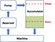
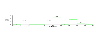
The oil pump example [3] was a real industrial case provided by the German company HYDAC ELECTRONICS GMBH, and studied at length within the European research project Quasimodo. The whole system, depicted by Fig. 2, consists of a machine, an accumulator, a reservoir and a pump. The machine consumes oil periodically out of the accumulator with a duration of 20s20𝑠20\,s (second) for one consumption cycle. The profile of consumption rate is shown in Fig. 2. The pump adds oil from the reservoir into the accumulator with power 2.2l/s2.2𝑙𝑠2.2\,l/s (liter/second).

Refer to caption
Figure 1: The oil pump system. (This picture is based on [3].)
Refer to caption
Figure 2: Consumption rate of the machine in one cycle.

Control objectives for this system are: by switching on/off the pump at certain time points

0t1t2tntn+1,0subscript𝑡1subscript𝑡2subscript𝑡𝑛subscript𝑡𝑛10\leq t_{1}\leq t_{2}\leq\cdots\leq t_{n}\leq t_{n+1}\leq\cdots\,, (7)

ensure that

  • \bullet

    RssubscriptRs\mathrm{R_{s}} (safety):  the system can run arbitrarily long while maintaining v(t)𝑣𝑡v(t) within [Vmin,Vmax]subscript𝑉subscript𝑉[V_{\min},V_{\max}] for any time point t𝑡t, where v(t)𝑣𝑡v(t) denotes the oil volume in the accumulator at time t𝑡t, Vmin=4.9lsubscript𝑉4.9𝑙V_{\min}=4.9\,l (liter) and Vmax=25.1lsubscript𝑉25.1𝑙V_{\max}=25.1\,l ;

and considering the energy cost and wear of the system, a second objective:

  • \bullet

    RosubscriptRo\mathrm{R_{o}} (optimality):  minimize the average accumulated oil volume in the limit, i.e. minimize

    limT1Tt=0Tv(t)dt.subscript𝑇1𝑇superscriptsubscript𝑡0𝑇𝑣𝑡differential-d𝑡\lim_{T\rightarrow\infty}\frac{1}{T}\int_{t=0}^{T}v(t){\mathrm{d}}t\enspace.

Both objectives should be achieved under two additional constraints:

  • \bullet

    RplsubscriptRpl\mathrm{R_{pl}} (pump latency):  there must be a latency of at least 2s2𝑠2\,s between any two consecutive operations of the pump; and

  • \bullet

    RrsubscriptRr\mathrm{R_{r}} (robustness):  uncertainty of the system should be taken into account:

    • -

      fluctuation of consumption rate (if it is not 00), up to f=0.1l/s𝑓0.1𝑙𝑠f=0.1\,l/s ;

    • -

      imprecision in the measurement of oil volume, up to ϵ=0.06litalic-ϵ0.06𝑙\epsilon=0.06\,l ;

    • -

      imprecision in the measurement of time, up to δ=0.015s𝛿0.015𝑠\delta=0.015\,s.333In [3], δ𝛿\delta is assumed to be 0.010.010.01. Here we include an extra rounding error of 0.0050.0050.005 due to floating point calculations in the implementation of our control strategy.

In [3], the authors used timed game automata to model the above system, and applied the tool UPPAAL-TIGA to synthesize near-optimal controllers. Due to discretization made in the timed-game model, an incorrect controller might be synthesized. Therefore the correctness and robustness of the synthesized controllers are checked using the tool PHAVER. Through simulations in SIMULINK, it was shown that the controllers synthesized by UPPAAL-TIGA provides big improvement (about 40%percent4040\%) over the Bang-Bang Controller and Smart Controller that are currently used at the HYDAC company. We will show how further improvement can be achieved using our approach.

4 Deriving Constraints from Safety Requirements

Following [3], the determination of control points (7) can be localized by exploiting the periodicity of oil consumption. That is, decisions on when to switch on/off the pump in one cycle can be made locally by measuring the initial oil volume v0subscript𝑣0v_{0} at the beginning of each cycle. Accordingly, the safety requirement RssubscriptRs\mathrm{R}_{\mathrm{s}} in Section 3 can be reformulated as: find an interval [L,U][Vmin,Vmax]𝐿𝑈subscript𝑉subscript𝑉[L,U]\subseteq[V_{\min},V_{\max}] s.t.

  • \bullet

    RlusubscriptRlu\mathrm{R_{lu}} (constraint for L,U𝐿𝑈L,U):  for all v0[L,U]subscript𝑣0𝐿𝑈v_{0}\in[L,U], there is a finite sequence of time points 𝐭=(t1,t2,,tn),𝐭subscript𝑡1subscript𝑡2subscript𝑡𝑛\mathbf{t}=(t_{1},t_{2},\ldots,t_{n})\,,444The choice of n𝑛n will be made later (in this paper n𝑛n can be 0,2,4,602460,2,4,6), but larger n𝑛n’s obviously will have the potential of allowing improved controllers. where 0t1t2tn200subscript𝑡1subscript𝑡2subscript𝑡𝑛200\leq t_{1}\leq t_{2}\leq\ldots\leq t_{n}\leq 20 satisfy RplsubscriptRpl\mathrm{R_{pl}}, for turning on/off the pump so that the resulting v(t)𝑣𝑡v(t) with v(0)=v0𝑣0subscript𝑣0v(0)=v_{0} satisfies

    • \scriptstyle{\bullet}

      RisubscriptRi\mathrm{R_{i}} (inductiveness):  v(20)[L,U]𝑣20𝐿𝑈v(20)\in[L,U]; and

    • \scriptstyle{\bullet}

      RlssubscriptRls\mathrm{R_{ls}} (local safety):  v(t)[Vmin,Vmax]𝑣𝑡subscript𝑉subscript𝑉v(t)\in[V_{\min},V_{\max}] for all t[0,20]𝑡020t\in[0,20]

    under constraint RrsubscriptRr\mathrm{R_{r}}.

Definition 1 (Local Controller)

The above 𝐭𝐭\mathbf{t} corresponding to v0subscript𝑣0v_{0} is called a local controller; the interval [L,U]𝐿𝑈[L,U] is called a stable interval.

Basically, RlusubscriptRlu\mathrm{R_{lu}} says that there is a stable interval [L,U]𝐿𝑈[L,U] and a corresponding family of local control strategies which can be repeated for arbitrarily many cycles and guarantee safety in each cycle.

4.0.1 Modeling Oil Consumption.

Let Vout(t)subscript𝑉𝑜𝑢𝑡𝑡V_{out}(t) with Vout(0)=0subscript𝑉𝑜𝑢𝑡00V_{out}(0)=0 denote the amount of oil consumed by time t𝑡t in one cycle, and modify the consumption rate in Fig. 2 by f𝑓f in (RrsubscriptRr\mathrm{R_{r}}). Then by simply integrating the lower and upper bounds of the consumption rate over the time interval [0,20]020[0,20] we can get

C1=^(0t2Vout=0)(2t41.1(t2)Vout1.3(t2))(4t82.2Vout2.6)(8t102.2+1.1(t8)Vout2.6+1.3(t8))(10t124.4+2.4(t10)Vout5.2+2.6(t10))(12t149.2Vout10.4)(14t169.2+1.6(t14)Vout10.4+1.8(t14))(16t1812.4+0.4(t16)Vout14+0.6(t16))(18t2013.2Vout15.2).C_{1}\,\widehat{=}\,\,\,\begin{array}[]{lll}\,\,\,\,\scriptstyle(0\leq t\leq 2&\scriptstyle\longrightarrow&\scriptstyle V_{out}=0)\\ \scriptstyle\wedge\,(2\leq t\leq 4&\scriptstyle\longrightarrow&\scriptstyle 1.1(t-2)\leq V_{out}\leq 1.3(t-2))\\ \scriptstyle\wedge\,(4\leq t\leq 8&\scriptstyle\longrightarrow&\scriptstyle 2.2\leq V_{out}\leq 2.6)\\ \scriptstyle\wedge\,(8\leq t\leq 10&\scriptstyle\longrightarrow&\scriptstyle 2.2+1.1(t-8)\leq V_{out}\leq 2.6+1.3(t-8))\\ \scriptstyle\wedge\,(10\leq t\leq 12&\scriptstyle\longrightarrow&\scriptstyle 4.4+2.4(t-10)\leq V_{out}\leq 5.2+2.6(t-10))\\ \scriptstyle\wedge\,(12\leq t\leq 14&\scriptstyle\longrightarrow&\scriptstyle 9.2\leq V_{out}\leq 10.4)\\ \scriptstyle\wedge\,(14\leq t\leq 16&\scriptstyle\longrightarrow&\scriptstyle 9.2+1.6(t-14)\leq V_{out}\leq 10.4+1.8(t-14))\\ \scriptstyle\wedge\,(16\leq t\leq 18&\scriptstyle\longrightarrow&\scriptstyle 12.4+0.4(t-16)\leq V_{out}\leq 14+0.6(t-16))\\ \scriptstyle\wedge\,(18\leq t\leq 20&\scriptstyle\longrightarrow&\scriptstyle 13.2\leq V_{out}\leq 15.2)\end{array}\enspace.

Actually, if the machine consuming oil is regarded as a hybrid system \mathcal{H} with state variable Voutsubscript𝑉𝑜𝑢𝑡V_{out} and continuous dynamics subject to box constraints, then C1subscript𝐶1C_{1} is the exact reachable set of \mathcal{H} from initial point Vout=0subscript𝑉𝑜𝑢𝑡0V_{out}=0 within 20 time units. Therefore we do not need to approximate the reachable set of \mathcal{H} by generating inductive invariants. This is also the case with the following pump system. However, if the consumption profile is more complicated, say piecewise polynomial, then approximations are indeed necessary.

4.0.2 Modeling Pump.

In [3] it is assumed that the number of activations of pump in one cycle is at most 2. We will adopt this assumption at first and increase this number later on. With this assumption, there will be at most four time points to switch the pump on/off in one cycle, denoted by 0t1t2t3t4200subscript𝑡1subscript𝑡2subscript𝑡3subscript𝑡4200\leq t_{1}\leq t_{2}\leq t_{3}\leq t_{4}\leq 20. If the pump is started only once or zero times, then we just set t3=t4=20subscript𝑡3subscript𝑡420t_{3}=t_{4}=20 or t1=t2=t3=t4=20subscript𝑡1subscript𝑡2subscript𝑡3subscript𝑡420t_{1}=t_{2}=t_{3}=t_{4}=20 respectively. Then the 2-second latency requirement (RplsubscriptRpl\mathrm{R_{pl}}) can be modeled by

C2=^(t12t2t12t3t22t4t32t420)(t12t2t12t220t3=20t4=20)(t1=20t2=20t3=20t4=20).subscript𝐶2^subscript𝑡12subscript𝑡2subscript𝑡12subscript𝑡3subscript𝑡22subscript𝑡4subscript𝑡32subscript𝑡420subscript𝑡12subscript𝑡2subscript𝑡12subscript𝑡220subscript𝑡320subscript𝑡420subscript𝑡120subscript𝑡220subscript𝑡320subscript𝑡420C_{2}\,\widehat{=}\,\,\,\begin{array}[]{l}\,\,\,\,\scriptstyle(t_{1}\geq 2\,\wedge\,t_{2}-t_{1}\geq 2\,\wedge\,t_{3}-t_{2}\geq 2\,\wedge\,t_{4}-t_{3}\geq 2\,\wedge\,t_{4}\leq 20)\\ \scriptstyle\vee\,(t_{1}\geq 2\,\wedge\,t_{2}-t_{1}\geq 2\,\wedge\,t_{2}\leq 20\,\wedge\,t_{3}=20\,\wedge\,t_{4}=20)\\ \scriptstyle\vee\,(t_{1}=20\,\wedge\,t_{2}=20\,\wedge\,t_{3}=20\,\wedge\,t_{4}=20)\\ \end{array}\enspace.

Let Vin(t)subscript𝑉𝑖𝑛𝑡V_{in}(t) with Vin(0)=0subscript𝑉𝑖𝑛00V_{in}(0)=0 denote the amount of oil introduced into the accumulator by time t𝑡t in one cycle. Then we have

C3=^(0tt1Vin=0)(t1tt2Vin=2.2(tt1))(t2tt3Vin=2.2(t2t1))(t3tt4Vin=2.2(t2t1)+2.2(tt3))(t4t20Vin=2.2(t2+t4t1t3)).C_{3}\,\widehat{=}\,\,\,\begin{array}[]{lll}\,\,\,\,\scriptstyle(0\leq t\leq t_{1}&\scriptstyle\longrightarrow&\scriptstyle V_{in}=0)\\ \scriptstyle\wedge\,(t_{1}\leq t\leq t_{2}&\scriptstyle\longrightarrow&\scriptstyle V_{in}=2.2(t-t_{1}))\\ \scriptstyle\wedge\,(t_{2}\leq t\leq t_{3}&\scriptstyle\longrightarrow&\scriptstyle V_{in}=2.2(t_{2}-t_{1}))\\ \scriptstyle\wedge\,(t_{3}\leq t\leq t_{4}&\scriptstyle\longrightarrow&\scriptstyle V_{in}=2.2(t_{2}-t_{1})+2.2(t-t_{3}))\\ \scriptstyle\wedge\,(t_{4}\leq t\leq 20&\scriptstyle\longrightarrow&\scriptstyle V_{in}=2.2(t_{2}+t_{4}-t_{1}-t_{3}))\\ \end{array}\enspace.

4.0.3 Encoding Safety Requirements.

Denote the oil volume in the accumulator at the beginning of one cycle by v0subscript𝑣0v_{0}, and the volume at time t𝑡t by v(t)𝑣𝑡v(t). Then for any 0t200𝑡200\leq t\leq 20 we have:

C4=^v=v0+VinVout.subscript𝐶4^𝑣subscript𝑣0subscript𝑉𝑖𝑛subscript𝑉𝑜𝑢𝑡C_{4}\,\widehat{=}\,\,v=v_{0}+V_{in}-V_{out}\enspace.

According to (RrsubscriptRr\mathrm{R_{r}}), the measurement of tisubscript𝑡𝑖t_{i} (1i41𝑖41\leq i\leq 4) and v0subscript𝑣0v_{0} may deviate from their actual values, so v(t)𝑣𝑡v(t) will deviate from its predicted value as stated in the requirement C4subscript𝐶4C_{4}. Nevertheless, we have the following estimation of the deviation of v(t)𝑣𝑡v(t).

Lemma 1

Let v~(t)~𝑣𝑡\tilde{v}(t) denote the actual oil volume in the accumulator at time t𝑡t. Then for any 0t200𝑡200\leq t\leq 20, |v(t)v~(t)|8.8δ+ϵ<0.2.𝑣𝑡~𝑣𝑡8.8𝛿italic-ϵ0.2|v(t)-\tilde{v}(t)|\leq 8.8\,\delta+\epsilon<0.2.

Proof

By (RrsubscriptRr\mathrm{R_{r}}) and C4subscript𝐶4C_{4}, v0subscript𝑣0v_{0} will cause an imprecision of ϵitalic-ϵ\epsilon and each tisubscript𝑡𝑖t_{i} will cause an imprecision of 2.2δ2.2𝛿2.2\,\delta . ∎

By Lemma 1, it is sufficient to rectify the safety bounds in (RisubscriptRi\mathrm{R_{i}}) and (RlssubscriptRls\mathrm{R_{ls}}) by an amount of 0.20.20.2. Let

C5=^t=20L+0.2vU0.2C6=^0t20Vmin+0.2vVmax0.2.subscript𝐶5^𝑡20𝐿0.2𝑣𝑈0.2subscript𝐶6^0𝑡20subscript𝑉0.2𝑣subscript𝑉0.2\begin{array}[]{lll}C_{5}&\,\widehat{=}&\,\,t=20\longrightarrow L+0.2\leq v\leq U-0.2\\ C_{6}&\,\widehat{=}&\,\,0\leq t\leq 20\longrightarrow V_{\min}+0.2\leq v\leq V_{\max}-0.2\enspace.\end{array}

Then (RisubscriptRi\mathrm{R_{i}}) and (RlssubscriptRls\mathrm{R_{ls}}) can be expressed as

𝒮=^t,v,Vin,Vout.(C1C3C4C5C6).formulae-sequence𝒮^for-all𝑡𝑣subscript𝑉𝑖𝑛subscript𝑉𝑜𝑢𝑡subscript𝐶1subscript𝐶3subscript𝐶4subscript𝐶5subscript𝐶6\mathcal{S}\,\widehat{=}\,\forall t,v,V_{in},V_{out}.(C_{1}\wedge C_{3}\wedge C_{4}\longrightarrow C_{5}\wedge C_{6})\,.

4.0.4 Deriving Constraints.

To find such [L,U]𝐿𝑈[L,U] that for every v0[L,U]subscript𝑣0𝐿𝑈v_{0}\in[L,U] there is a local control strategy satisfying RisubscriptRi\mathrm{R_{i}} and RlssubscriptRls\mathrm{R_{ls}}, let

C7=^Lv0U,subscript𝐶7^𝐿subscript𝑣0𝑈C_{7}\,\widehat{=}\,\,L\leq v_{0}\leq U\enspace,

and then RlusubscriptRlu\mathrm{R_{lu}} can be encoded into

C8=^v0.(C7t1t2t3t4.(C2𝒮)).\begin{array}[]{l}C_{8}\,\widehat{=}\,\forall v_{0}.\Big{(}C_{7}\longrightarrow\exists t_{1}t_{2}t_{3}t_{4}.\big{(}C_{2}\,\wedge\mathcal{S}\big{)}\Big{)}\end{array}\,.

We use the tool Mjollnir [18] to do QE on C8subscript𝐶8C_{8} and the following result is returned:

C9=^L5.1U24.9UL2.4.subscript𝐶9^𝐿5.1𝑈24.9𝑈𝐿2.4C_{9}\,\widehat{=}\,L\geq 5.1\wedge U\leq 24.9\wedge U-L\geq 2.4\enspace.

Then the relation between L,U,v0𝐿𝑈subscript𝑣0L,U,v_{0} and the corresponding local control strategy 𝐭=(t1,t2,t3,t4)𝐭subscript𝑡1subscript𝑡2subscript𝑡3subscript𝑡4\mathbf{t}=(t_{1},t_{2},t_{3},t_{4}) can be obtained by applying QE to

C10=^C2C7C9𝒮.subscript𝐶10^subscript𝐶2subscript𝐶7subscript𝐶9𝒮C_{10}\,\widehat{=}\,C_{2}\wedge C_{7}\wedge C_{9}\,\wedge\mathcal{S}\,.

The result given by Mjollnir, when converted to DNF, is a disjunction of 92 components:

𝒟(L,U,v0,t1,t2,t3,t4)=^i=192Di𝒟𝐿𝑈subscript𝑣0subscript𝑡1subscript𝑡2subscript𝑡3subscript𝑡4^superscriptsubscript𝑖192subscript𝐷𝑖\mathcal{D}(L,U,v_{0},t_{1},t_{2},t_{3},t_{4})\,\widehat{=}\,\bigvee_{i=1}^{92}D_{i}

(denoted by 𝒟𝒟\mathcal{D} for short), with each Disubscript𝐷𝑖D_{i} representing a nonempty closed convex polyhedron (see Appendix 0.A.1).666The fact that each Disubscript𝐷𝑖D_{i} is a nonempty closed set can be checked using QE.

5 A “Hybrid” Approach for Optimization

5.1 Encoding of the Optimization Objective

By Definition 1, the optimal average accumulated oil volume in RosubscriptRo\mathrm{R_{o}} can be redefined as

Ro:min[L,U]maxv0[L,U]min𝐭120t=020v(t)dt.\bullet\,\,\,\mathrm{R_{o}^{\prime}:}\quad\quad\min_{\scriptscriptstyle{[L,U]}}\,\max_{\scriptscriptstyle{v_{0}\in[L,U]}}\,\min_{\mathbf{t}}\,\frac{1}{20}\int_{t=0}^{20}v(t)\mathrm{d}t\enspace. (8)

The intuitive meaning of (RosuperscriptsubscriptRo\mathrm{R_{o}^{\prime}}) is:

  • for each admissible [L,U]𝐿𝑈[L,U] and each v0[L,U]subscript𝑣0𝐿𝑈v_{0}\in[L,U], minimize the average accumulated oil volume in one cycle, i.e. 120t=020v(t)dt120superscriptsubscript𝑡020𝑣𝑡differential-d𝑡\frac{1}{20}\int_{t=0}^{20}v(t)\mathrm{d}t, over all admissible local controllers 𝐭𝐭\mathbf{t};

  • fix [L,U]𝐿𝑈[L,U] and select the worst local minimum by traversing all v0[L,U]subscript𝑣0𝐿𝑈v_{0}\in[L,U];

  • then the global minimum is obtained at the interval whose worst local minimum is minimal.

Definition 2 (Local Optimal Controller)

Let 𝒟𝐭=^{𝐭(L,U,v0,𝐭)𝒟}subscript𝒟𝐭^conditional-set𝐭𝐿𝑈subscript𝑣0𝐭𝒟\mathcal{D}_{\mathbf{t}}\,\widehat{=}\,\{\mathbf{t}\mid(L,U,v_{0},\mathbf{t})\in\mathcal{D}\} for fixed L,U,v0𝐿𝑈subscript𝑣0L,U,v_{0}. Then we call

min𝐭𝒟𝐭120t=020v(t)dtsubscript𝐭subscript𝒟𝐭120superscriptsubscript𝑡020𝑣𝑡differential-d𝑡\min_{\mathbf{t}\in\mathcal{D}_{\mathbf{t}}}\,\frac{1}{20}\int_{t=0}^{20}v(t)\mathrm{d}t

the optimal local average accumulated oil volume corresponding to L,U,v0𝐿𝑈subscript𝑣0L,U,v_{0}, and the optimizer 𝐭𝐭\mathbf{t} is called the local optimal controller.

Let g(v0,t1,t2,t3,t4)=^120t=020v(t)dt𝑔subscript𝑣0subscript𝑡1subscript𝑡2subscript𝑡3subscript𝑡4^120superscriptsubscript𝑡020𝑣𝑡differential-d𝑡g(v_{0},t_{1},t_{2},t_{3},t_{4})\,\widehat{=}\,\frac{1}{20}\int_{t=0}^{20}v(t)\mathrm{d}t, denoted by g𝑔g for short. Then it can be computed from C1,C3,C4subscript𝐶1subscript𝐶3subscript𝐶4C_{1},C_{3},C_{4} without considering fluctuations of consumption rate that

g=20v0+1.1(t12t22+t32t4240t1+40t240t3+40t4)132.220.𝑔20subscript𝑣01.1superscriptsubscript𝑡12superscriptsubscript𝑡22superscriptsubscript𝑡32superscriptsubscript𝑡4240subscript𝑡140subscript𝑡240subscript𝑡340subscript𝑡4132.220g\,=\,\frac{20v_{0}+1.1(t_{1}^{2}-t_{2}^{2}+t_{3}^{2}-t_{4}^{2}-40t_{1}+40t_{2}-40t_{3}+40t_{4})-132.2}{20}\enspace.

Then by Proposition 1, (RosuperscriptsubscriptRo\mathrm{R_{o}^{\prime}}) can be encoded into

L,U.(C9v0.(C7t1t2t3t4.(𝒟gz))),\exists L,U.\Big{(}C_{9}\wedge\,\forall v_{0}.\big{(}C_{7}\longrightarrow\exists t_{1}t_{2}t_{3}t_{4}.(\mathcal{D}\wedge g\leq z)\big{)}\Big{)}\,, (9)

which is equivalent to zz𝑧superscript𝑧z\geq z^{*} or z>z𝑧superscript𝑧z>z^{*}, where zsuperscript𝑧z^{*} equals the value of (8).

5.2 Techniques for Performing QE

The above deduced (9) is a huge formula with nonlinear terms and two alternations of quantifiers, for which direct QE fails. Therefore we have made our efforts to decompose the QE problem into manageable parts.

5.2.1 Eliminating the Inner Quantifiers.

We first eliminate the innermost quantified variables t1t2t3t4subscript𝑡1subscript𝑡2subscript𝑡3subscript𝑡4\exists t_{1}t_{2}t_{3}t_{4} by employing the theory of quadratic programming.

Note that Disubscript𝐷𝑖D_{i} in 𝒟𝒟\mathcal{D} is a closed convex polyhedron for all i𝑖i and g𝑔g is a quadratic polynomial function, so minimization of g𝑔g on Disubscript𝐷𝑖D_{i} is a quadratic programming problem. Then the Karush-Kuhn-Tucker (KKT) [13] condition

θkkt=^𝝁.(g,Di),formulae-sequencesubscript𝜃kkt^𝝁𝑔subscript𝐷𝑖\theta_{\mathrm{kkt}}\,\,\widehat{=}\,\,\,\exists\boldsymbol{\mu}.\,\mathcal{L}(g,D_{i})\,, (10)

where (g,Di)𝑔subscript𝐷𝑖\mathcal{L}(g,D_{i}) is a linear formula constructed from g𝑔g and Disubscript𝐷𝑖D_{i}, and 𝝁𝝁\boldsymbol{\mu} is a vector of new variables, gives a necessary condition for a local minimum of g𝑔g on Disubscript𝐷𝑖D_{i}.

By applying the KKT condition to each Disubscript𝐷𝑖D_{i} and eliminating all 𝝁𝝁\boldsymbol{\mu}, we can get a necessary condition 𝒟superscript𝒟\mathcal{D}^{\prime}, a disjunction of 580 parts, for the minimum of g𝑔g on 𝒟𝒟\mathcal{D}:

𝒟=j=1580Bj.superscript𝒟superscriptsubscript𝑗1580subscript𝐵𝑗\mathcal{D}^{\prime}=\bigvee_{j=1}^{580}B_{j}\,.

Furthermore, each Bjsubscript𝐵𝑗B_{j} has the nice property that for any L,U,v0𝐿𝑈subscript𝑣0L,U,v_{0}, a unique 𝐭jsubscript𝐭𝑗\mathbf{t}_{j} is determined by Bjsubscript𝐵𝑗B_{j} (see Appendix 0.A.2).777This has been verified by QE. For instance, one of the Bjsubscript𝐵𝑗B_{j} reads:

t4=2016t2+10L349=0t2t3+2=022t116t210v0+107=0.subscript𝑡42016subscript𝑡210𝐿349limit-from0subscript𝑡2subscript𝑡32022subscript𝑡116subscript𝑡210subscript𝑣01070\begin{array}[]{l}t_{4}=20\wedge 16t_{2}+10L-349=0\,\wedge\\ t_{2}-t_{3}+2=0\wedge 22t_{1}-16t_{2}-10v_{0}+107=0\,\wedge\cdots\\ \end{array}\enspace. (11)

Since 𝒟superscript𝒟\mathcal{D}^{\prime} keeps the minimal value point of g𝑔g on 𝒟𝒟\mathcal{D}, the formula obtained by replacing 𝒟𝒟\mathcal{D} by 𝒟superscript𝒟\mathcal{D}^{\prime} in (9)

L,U.(C9v0.(C7t1t2t3t4.(𝒟gz)))\exists L,U.\Big{(}C_{9}\wedge\,\forall v_{0}.\big{(}C_{7}\longrightarrow\exists t_{1}t_{2}t_{3}t_{4}.(\mathcal{D}^{\prime}\wedge g\leq z)\big{)}\Big{)}\, (12)

is equivalent to (9). Then according to formulas like (11), t1t2t3t4subscript𝑡1subscript𝑡2subscript𝑡3subscript𝑡4\exists t_{1}t_{2}t_{3}t_{4} in (12) can be eliminated by the distribution of \exists among disjunctions, followed by instantiations of 𝐭jsubscript𝐭𝑗\mathbf{t}_{j} in each disjunct. Thus (9) can be converted to

L,U.(C9v0.(C7j=1580(Ajgjz))),\exists L,U.\Big{(}C_{9}\wedge\forall v_{0}.\big{(}C_{7}\longrightarrow\bigvee_{j=1}^{580}(A_{j}\wedge g_{j}\leq z)\big{)}\Big{)}\enspace, (13)

where Ajsubscript𝐴𝑗A_{j} is a constraint on L,U,v0𝐿𝑈subscript𝑣0L,U,v_{0}, and gjsubscript𝑔𝑗g_{j} is the instantiation of g𝑔g using 𝐭jsubscript𝐭𝑗\mathbf{t}_{j} given by formulas like (11).

5.2.2 Eliminating the Outer Quantifiers.

We eliminate the outermost quantifiers L,U𝐿𝑈\exists L,U in (13) by discretization, as discussed in Section 2.

According to C9subscript𝐶9C_{9}, the interval [5.1,24.9]5.124.9[5.1,24.9] is discretized with a granularity of 0.10.10.1, which gives a set of 199199199 elements. Then assignments to L,U𝐿𝑈L,U from this set satisfying C9subscript𝐶9C_{9} are used to instantiate (13). There are totally 154001540015400 such pairs of L,U𝐿𝑈L,U, e.g. (5.1,7.5)5.17.5(5.1,7.5), (5.1,7.6)5.17.6(5.1,7.6) etc, and as many instantiations in the form of

v0.(C7j=1580(Ajgjz)),formulae-sequencefor-allsubscript𝑣0subscript𝐶7superscriptsubscript𝑗1580subscript𝐴𝑗subscript𝑔𝑗𝑧\forall v_{0}.\big{(}C_{7}\longrightarrow\bigvee_{j=1}^{580}(A_{j}\wedge g_{j}\leq z)\big{)}\enspace, (14)

each of which gives an optimal value corresponding to [L,U]𝐿𝑈[L,U]. In practice, we start from L=5.1,U=7.5formulae-sequence𝐿5.1𝑈7.5L=5.1,U=7.5, and search for the minimal optimal value through all the 154001540015400 cases with L𝐿L or U𝑈U incremented by 0.10.10.1 every iteration.

5.2.3 Eliminating the Middle Quantifier.

We finally eliminate the only quantifier left in (14) by a divide-and-conquer strategy. First, we can show that

Lemma 2

j=1580Ajsuperscriptsubscript𝑗1580subscript𝐴𝑗\bigvee_{j=1}^{580}A_{j} is equivalent to C7subscript𝐶7C_{7} in (14).

Proof

As discussed above,

𝐭.(𝒟gz)𝐭.(𝒟gz)j=1580(Ajgjz).\exists\mathbf{t}.(\mathcal{D}\wedge g\leq z)\Leftrightarrow\exists\mathbf{t}.(\mathcal{D}^{\prime}\wedge g\leq z)\Leftrightarrow\bigvee_{j=1}^{580}(A_{j}\wedge g_{j}\leq z)\enspace.

Therefore

z𝐭.(𝒟gz)z.j=1580(Ajgjz).\exists z\exists\mathbf{t}.(\mathcal{D}\wedge g\leq z)\Leftrightarrow\exists z.\bigvee_{j=1}^{580}(A_{j}\wedge g_{j}\leq z)\enspace.

By eliminating z𝑧z we have 𝐭.𝒟j=1580Aj\exists\mathbf{t}.\mathcal{D}\Leftrightarrow\bigvee_{j=1}^{580}A_{j}. According to C8subscript𝐶8C_{8} and C10subscript𝐶10C_{10}, 𝒟𝒟\mathcal{D} has been chosen in such a way that for any v0[L,U]subscript𝑣0𝐿𝑈v_{0}\in[L,U] there is a local controller 𝐭𝐭\mathbf{t}. Thus 𝐭.𝒟C7\exists\mathbf{t}.\mathcal{D}\Leftrightarrow C_{7} when L,U𝐿𝑈L,U are instantiated.∎

By this lemma if all Ajsubscript𝐴𝑗A_{j} are pairwise disjoint then (14) is equivalent to

j=1580v0.(v0Aj(Ajgjz)).formulae-sequencesuperscriptsubscript𝑗1580for-allsubscript𝑣0subscript𝑣0subscript𝐴𝑗subscript𝐴𝑗subscript𝑔𝑗𝑧\bigwedge_{j=1}^{580}\forall v_{0}.\big{(}v_{0}\in A_{j}\longrightarrow(A_{j}\wedge g_{j}\leq z)\big{)}\,. (15)

Since each conjunct in (15) is a small formula with only two variables v0,zsubscript𝑣0𝑧v_{0},z and one universal quantifier, it can be dealt with quite efficiently.
Refer to caption
Refer to caption
Figure 3: Region partition.

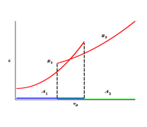
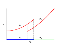
If the set of Ajsubscript𝐴𝑗A_{j}s are not pairwise disjoint, then we have to partition them into disjoint regions and assign a new cost function gksuperscriptsubscript𝑔𝑘g_{k}^{\prime} to each region. The idea for performing such partition is simple and is illustrated by Fig. 3.

Suppose two sets, say A1,A2subscript𝐴1subscript𝐴2A_{1},A_{2}, are chosen arbitrarily from the set of Ajsubscript𝐴𝑗A_{j}s. If A1A2=subscript𝐴1subscript𝐴2A_{1}\cap A_{2}=\emptyset, then we do nothing. Otherwise check wether g1g2subscript𝑔1subscript𝑔2g_{1}\leq g_{2} (or g2g1subscript𝑔2subscript𝑔1g_{2}\leq g_{1}) on A1A2subscript𝐴1subscript𝐴2A_{1}\cap A_{2}: if so, assign the smaller one, i.e. g1zsubscript𝑔1𝑧g_{1}\leq z (or g2zsubscript𝑔2𝑧g_{2}\leq z) to A1A2subscript𝐴1subscript𝐴2A_{1}\cap A_{2}; otherwise we simply assign (g1z)(g2z)subscript𝑔1𝑧subscript𝑔2𝑧(g_{1}\leq z)\vee(g_{2}\leq z) to A1A2subscript𝐴1subscript𝐴2A_{1}\cap A_{2}.

If at the same time of partitioning regions we also make a record of the local control strategy in each region, i.e. 𝐭jsubscript𝐭𝑗\mathbf{t}_{j}, then in the end we can get exactly the family of local optimal controllers corresponding to each v0subscript𝑣0v_{0}.

5.3 Results of QE

Various tools are available for doing QE. In our implementation, the SMT-based tool Mjollnir [19, 18] is chosen for QE on linear formulas, while REDLOG [6] implementing virtual substitution [17] is chosen for formulas with nonlinear terms. The computer algebra system REDUCE [11], of which REDLOG is an integral part, allows us to perform some programming tasks, e.g. region partition. Table 1 shows the performance of our approach. All experiments are done on a desktop running Linux with a 2.66 GHz CPU and 3 GB memory.

Table 1: Timing of different QE tasks.
formula C8subscript𝐶8C_{8} C10subscript𝐶10C_{10} θkktsubscript𝜃kkt\theta_{\mathrm{kkt}} (all 92) all the rest
tool  Mjollnir  Mjollnir  Mjollnir   Redlog/Reduce
time 8m8s 4m13s 31s <<1s
Remark

In Table 1, timing is in minutes (m) and seconds (s); in the last column, the time taken to get the first optimal value888For the model with 2 activations, this optimal value is only obtained at the 1st iteration. is less than 1 second, whereas all 15400 iterations will cost more than 10 hours (using a single computing process).

The final results are as follows:

  • The interval that produces the optimal value is [5.1,7.5]5.17.5[5.1,7.5].

  • The local optimal controller for v0[5.1,7.5]subscript𝑣05.17.5v_{0}\in[5.1,7.5] is

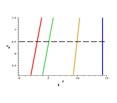
    t1=10v02513t2=10v0+113t3=10v0+15322t4=15711,subscript𝑡110subscript𝑣02513subscript𝑡210subscript𝑣0113subscript𝑡310subscript𝑣015322subscript𝑡415711t_{1}=\frac{10v_{0}-25}{13}\,\wedge\,t_{2}=\frac{10v_{0}+1}{13}\,\wedge\,t_{3}=\frac{10v_{0}+153}{22}\,\wedge\,t_{4}=\frac{157}{11}\enspace, (16)

    which is illustrated by Picture I in Fig. 4. If v0=6.5subscript𝑣06.5v_{0}=6.5, then by (16) the pump should be switched on at t1=40/13subscript𝑡14013t_{1}=40/13, off at t2=66/13subscript𝑡26613t_{2}=66/13, then on at t3=109/11subscript𝑡310911t_{3}=109/11, and finally off at t4=157/11subscript𝑡415711t_{4}=157/11.

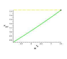
  • The optimal average accumulated oil volume 21527328600=7.53215273286007.53\frac{215273}{28600}=7.53 is obtained, improving by 5%percent55\% the optimal value 7.957.957.95 in [3], which is already a 40%percent4040\% improvement of the controllers from the HYDAC company. The local optimal average accumulated oil volume for v0[5.1,7.5]subscript𝑣05.17.5v_{0}\in[5.1,7.5] under controller (16), i.e. Vaav(v0)=1300v02+20420v0+634817114400subscript𝑉aavsubscript𝑣01300superscriptsubscript𝑣0220420subscript𝑣0634817114400\scriptstyle V_{\textit{aav}}(v_{0})\,=\,\frac{1300v_{0}^{2}+20420v_{0}+634817}{114400} , is illustrated by II of Fig. 4.

  • From II of Fig. 4 we can have an estimate of the performance of controller (16) in the long run. Without considering noises, it can be computed from (16) that v(20)=6.3𝑣206.3v(20)=6.3 no matter what v(0)𝑣0v(0) is, implying that the mean value of v0subscript𝑣0v_{0} equals 6.3. Therefore the mean average accumulated oil volume in the long run is Vaav(6.3)=407535720=7.125subscript𝑉aav6.34075357207.125V_{\textit{aav}}(6.3)=\frac{40753}{5720}=7.125. In [3], by simulating the oil pump system for a duration of 200s𝑠s, the mean values 7.447.447.44, 11.5611.5611.56 and 13.4513.4513.45 are obtained for the UPPAAL-TIGA controller, Smart Controller and Bang-Bang Controller respectively.
Refer to caption
Refer to caption
Figure 4: Optimal controllers and average accumulated oil volumes for 2 activations.

6 Improvement by Increasing Activation Times

In the controller shown by I of Fig. 4, we noticed that when v0subscript𝑣0v_{0} is small and the pump is started on for the second time, it stays on for a period longer than 4 seconds. Based on this observation, we conjecture that if the pump is allowed to be activated three times in one cycle, then each time it could stay on for a shorter period, and the time it is activated for the third time can be postponed. As a result, the accumulated oil volume in one cycle may become less.

To verify the above conjecture, some modifications must be made on the previous model. Firstly, C2subscript𝐶2C_{2} and C3subscript𝐶3C_{3} should be replaced

C2=^(t12t2t12t3t22t4t32t5t42t6t52t620)(t12t2t12t3t22t4t32t420t5=20t6=20)(t12t2t12t220t3=20t4=20t5=20t6=20)(t1=20t2=20t3=20t4=20t5=20t6=20)superscriptsubscript𝐶2^subscript𝑡12subscript𝑡2subscript𝑡12subscript𝑡3subscript𝑡22subscript𝑡4subscript𝑡32subscript𝑡5subscript𝑡42subscript𝑡6subscript𝑡52subscript𝑡620subscript𝑡12subscript𝑡2subscript𝑡12subscript𝑡3subscript𝑡22subscript𝑡4subscript𝑡32subscript𝑡420subscript𝑡520subscript𝑡620subscript𝑡12subscript𝑡2subscript𝑡12subscript𝑡220subscript𝑡320subscript𝑡420subscript𝑡520subscript𝑡620subscript𝑡120subscript𝑡220subscript𝑡320subscript𝑡420subscript𝑡520subscript𝑡620C_{2}^{\prime}\,\widehat{=}\,\begin{array}[]{l}\,\,\,\,{\scriptstyle(t_{1}\geq 2\,\wedge\,t_{2}-t_{1}\geq 2\,\wedge\,t_{3}-t_{2}\geq 2\,\wedge\,t_{4}-t_{3}\geq 2\,\wedge\,t_{5}-t_{4}\geq 2\,\wedge\,t_{6}-t_{5}\geq 2\,\wedge\,t_{6}\leq 20)}\\ \scriptstyle\vee\,{\scriptstyle(t_{1}\geq 2\,\wedge\,t_{2}-t_{1}\geq 2\,\wedge\,t_{3}-t_{2}\geq 2\,\wedge\,t_{4}-t_{3}\geq 2\,\wedge\,t_{4}\leq 20\,\wedge\,\,t_{5}=20\,\wedge\,t_{6}=20)}\\ \scriptstyle\vee\,{\scriptstyle(t_{1}\geq 2\,\wedge\,t_{2}-t_{1}\geq 2\,\wedge\,t_{2}\leq 20\,\wedge\,t_{3}=20\,\wedge\,t_{4}=20\,\wedge\,t_{5}=20\,\wedge\,t_{6}=20)}\\ \scriptstyle\vee\,{\scriptstyle(t_{1}=20\,\wedge\,t_{2}=20\,\wedge\,t_{3}=20\,\wedge\,t_{4}=20\,\wedge\,t_{5}=20\,\wedge\,t_{6}=20)}\end{array}

and

C3=^(0tt1Vin=0)(t1tt2Vin=2.2(tt1))(t2tt3Vin=2.2(t2t1))(t3tt4Vin=2.2(t2t1)+2.2(tt3))(t4tt5Vin=2.2(t2+t4t1t3))(t5tt6Vin=2.2(t2+t4t1t3)+2.2(tt5))(t6t20Vin=2.2(t2+t4+t6t1t3t5))C_{3}^{\prime}\,\widehat{=}\,\,\,\begin{array}[]{lll}\,\,\,\,{\scriptstyle(0\leq t\leq t_{1}}&\longrightarrow&\scriptstyle{V_{in}=0)}\\ \scriptstyle\wedge\,\scriptstyle(t_{1}\leq t\leq t_{2}&\longrightarrow&\scriptstyle V_{in}=2.2(t-t_{1}))\\ \scriptstyle\wedge\,\scriptstyle(t_{2}\leq t\leq t_{3}&\longrightarrow&\scriptstyle V_{in}=2.2(t_{2}-t_{1}))\\ \scriptstyle\wedge\,\scriptstyle(t_{3}\leq t\leq t_{4}&\longrightarrow&\scriptstyle V_{in}=2.2(t_{2}-t_{1})+2.2(t-t_{3}))\\ \scriptstyle\wedge\,\scriptstyle(t_{4}\leq t\leq t_{5}&\longrightarrow&\scriptstyle V_{in}=2.2(t_{2}+t_{4}-t_{1}-t_{3}))\\ \scriptstyle\wedge\,\scriptstyle(t_{5}\leq t\leq t_{6}&\longrightarrow&\scriptstyle V_{in}=2.2(t_{2}+t_{4}-t_{1}-t_{3})+2.2(t-t_{5}))\\ \scriptstyle\wedge\,\scriptstyle(t_{6}\leq t\leq 20&\longrightarrow&\scriptstyle V_{in}=2.2(t_{2}+t_{4}+t_{6}-t_{1}-t_{3}-t_{5}))\end{array}

respectively; secondly, in C5subscript𝐶5C_{5} and C6subscript𝐶6C_{6} the tolerance of noises should be increased to 0.30.30.3, because due to the increase of times to operate the pump, the maximal uncertainty caused by imprecision in measurement of volume and time is now 13.2δ+ϵ<0.313.2𝛿italic-ϵ0.313.2\delta+\epsilon<0.3; thirdly, the new objective function is

g=^20v0+1.1(t12t22+t32t42+t52t6240t1+40t240t3+40t440t5+40t6)132.220.𝑔^20subscript𝑣01.1superscriptsubscript𝑡12superscriptsubscript𝑡22superscriptsubscript𝑡32superscriptsubscript𝑡42superscriptsubscript𝑡52superscriptsubscript𝑡6240subscript𝑡140subscript𝑡240subscript𝑡340subscript𝑡440subscript𝑡540subscript𝑡6132.220\begin{array}[]{l}g\,\widehat{=}\,{\small{\frac{20v_{0}+1.1(t_{1}^{2}-t_{2}^{2}+t_{3}^{2}-t_{4}^{2}+t_{5}^{2}-t_{6}^{2}-40t_{1}+40t_{2}-40t_{3}+40t_{4}-40t_{5}+40t_{6})-132.2}{20}}}\end{array}\enspace.

For this model, we get the following results.

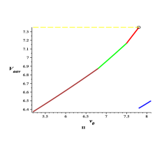
  • Using interval [5.2,8.1]5.28.1[5.2,8.1], the optimal average accumulated oil volume999The optimal value is first obtained at the 4th iteration, but there are many other intervals other than [5.2,8.1]5.28.1[5.2,8.1] that give the same optimal value 7.35. 6613900=7.3566139007.35\frac{6613}{900}=7.35 is obtained, which is a 7.5% improvement over the optimum 7.95 in [3].

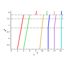
  • The local controllers for v0[5.2,8.1]subscript𝑣05.28.1v_{0}\in[5.2,8.1] is illustrated by I of Fig. 5:

    {t1=10v02613t2=10v013t3=5v0+7611t4=12t5=14t6=35922v0[5.2,6.8)t1=10v02613t2=10v013t3=5v0+7611t4=5v0+9811t5=5v0+929t6=20v0+3095198v0[6.8,7.5)t1=10v02613t2=10v013t3=5v0+7611t4=5v0+9811t5=5v0+929t6=5v0+1109v0[7.5,7.8)t1=10v0+2613t2=45v0+1300143t3=14t4=35922t5=20t6=20v0[7.8,8.1].casessubscript𝑡110subscript𝑣02613subscript𝑡210subscript𝑣013subscript𝑡35subscript𝑣07611subscript𝑡412subscript𝑡514subscript𝑡635922subscript𝑣05.26.8subscript𝑡110subscript𝑣02613subscript𝑡210subscript𝑣013subscript𝑡35subscript𝑣07611subscript𝑡45subscript𝑣09811subscript𝑡55subscript𝑣0929subscript𝑡620subscript𝑣03095198subscript𝑣06.87.5subscript𝑡110subscript𝑣02613subscript𝑡210subscript𝑣013subscript𝑡35subscript𝑣07611subscript𝑡45subscript𝑣09811subscript𝑡55subscript𝑣0929subscript𝑡65subscript𝑣01109subscript𝑣07.57.8subscript𝑡110subscript𝑣02613subscript𝑡245subscript𝑣01300143subscript𝑡314subscript𝑡435922subscript𝑡520subscript𝑡620subscript𝑣07.88.1\left\{\begin{array}[]{ll}{\scriptstyle{t_{1}=\frac{10v_{0}-26}{13}}\,\wedge\,t_{2}=\frac{10v_{0}}{13}\,\wedge\,t_{3}=\frac{5v_{0}+76}{11}\,\wedge\,t_{4}=12\,\wedge\,t_{5}=14\,\wedge\,t_{6}=\frac{359}{22}}&{\scriptstyle v_{0}\in[5.2,6.8)}\\ {\scriptstyle{t_{1}=\frac{10v_{0}-26}{13}}\,\wedge\,t_{2}=\frac{10v_{0}}{13}\,\wedge\,t_{3}=\frac{5v_{0}+76}{11}\,\wedge\,t_{4}=\frac{5v_{0}+98}{11}\,\wedge\,t_{5}=\frac{5v_{0}+92}{9}\,\wedge\,t_{6}=\frac{20v_{0}+3095}{198}}&{\scriptstyle v_{0}\in[6.8,7.5)}\\ {\scriptstyle{t_{1}=\frac{10v_{0}-26}{13}}\,\wedge\,t_{2}=\frac{10v_{0}}{13}\,\wedge\,t_{3}=\frac{5v_{0}+76}{11}\,\wedge\,t_{4}=\frac{5v_{0}+98}{11}\,\wedge\,t_{5}=\frac{5v_{0}+92}{9}\,\wedge\,t_{6}=\frac{5v_{0}+110}{9}}&{\scriptstyle v_{0}\in[7.5,7.8)}\\ {\scriptstyle{t_{1}=\frac{10v_{0}+26}{13}}\,\wedge\,t_{2}=\frac{45v_{0}+1300}{143}\,\wedge\,t_{3}=14\,\wedge\,t_{4}=\frac{359}{22}\,\wedge\,t_{5}=20\,\wedge\,t_{6}=20}&{\scriptstyle{v_{0}\in[7.8,8.1]}\,.}\end{array}\right.
  • The local optimal value for v0[5.2,8.1]subscript𝑣05.28.1v_{0}\in[5.2,8.1] is illustrated by II of Fig. 5, from which it can be estimated that the mean average accumulated oil volume in the long run is around 6.86.86.8.

Refer to caption
Refer to caption
Figure 5: Optimal controllers and average accumulated oil volumes for 3 activations.

Furthermore, the following theorem indicates that the theoretically optimal controller can be obtained using the local control strategy with three activations. Therefore, our approach in fact gives the theoretically optimal controller in the oil pump industrial example.

Theorem 6.1

For each admissible [L,U]𝐿𝑈[L,U], each v0[L,U]subscript𝑣0𝐿𝑈v_{0}\in[L,U], and any local control strategy s4subscript𝑠4s_{4} with at least 4 activations subject to Rlusubscript𝑅𝑙𝑢R_{lu}, Risubscript𝑅𝑖R_{i} and Rlssubscript𝑅𝑙𝑠R_{ls}, there exists a local control strategy s3subscript𝑠3s_{3} subject to Rlusubscript𝑅𝑙𝑢R_{lu}, Risubscript𝑅𝑖R_{i} and Rlssubscript𝑅𝑙𝑠R_{ls} with 3 activations such that 120t=020vs3(t)dt<120t=020vs4(t)dt120superscriptsubscript𝑡020subscript𝑣subscript𝑠3𝑡differential-d𝑡120superscriptsubscript𝑡020subscript𝑣subscript𝑠4𝑡differential-d𝑡\,\frac{1}{20}\int_{t=0}^{20}v_{s_{3}}(t)\mathrm{d}t<\,\frac{1}{20}\int_{t=0}^{20}v_{s_{4}}(t)\mathrm{d}t, where vs3(t)subscript𝑣subscript𝑠3𝑡v_{s_{3}}(t) (resp. vs4(t)subscript𝑣subscript𝑠4𝑡v_{s_{4}}(t)) is the oil volume in the accumulator at t𝑡t with s3subscript𝑠3s_{3} (resp. s4subscript𝑠4s_{4}).

Proof

From the consumption rate of the machine in Fig. 2 and the behavior of the pump, we only need to consider a controller s4subscript𝑠4s_{4} that turns on the pump 4 times in a circle in order to guarantee Rlusubscript𝑅𝑙𝑢R_{lu}, Risubscript𝑅𝑖R_{i} and Rlssubscript𝑅𝑙𝑠R_{ls}. Furthermore, by Fig. 2, it is easy to argue that turning on the pump can only take place in the intervals [2,4]24[2,4], [8,12]812[8,12] and [14,20]1420[14,20] in order to obtain an optimal local control strategy; otherwise, a better local control strategy can be constructed just by postponing the activation time accordingly. In addition, we can further show that the pump can only be turned on at most once in the interval [8,12]812[8,12] for any optimal local control strategy. Now suppose we have an optimal local control strategy s4subscript𝑠4s_{4} that needs to turn on the pump four times in a circle in order to guarantee Rlusubscript𝑅𝑙𝑢R_{lu}, Risubscript𝑅𝑖R_{i} and Rlssubscript𝑅𝑙𝑠R_{ls}. Then by the above analysis, s4subscript𝑠4s_{4} switches the pump on respectively in [2,4]24[2,4], [8,12]812[8,12], at 14 for 2 seconds and at 18 for another 2 seconds. If not, it is easy to show the strategy is not optimal by contradiction. Now, let us construct a local control strategy s3subscript𝑠3s_{3} that turns on the pump three times in a circle as follows: its first two activation time are the same as the counterparts of s4subscript𝑠4s_{4}’s, but last ϵitalic-ϵ\epsilon seconds longer by considering noise, and it turns on the pump the third time at 14 for 3.2+ϵ3.2italic-ϵ3.2+\epsilon seconds, where ϵitalic-ϵ\epsilon is the noise (0.1 in this paper). By a simple calculation, it is easy to see that s3subscript𝑠3s_{3} satisfies Rlusubscript𝑅𝑙𝑢R_{lu}, Risubscript𝑅𝑖R_{i} and Rlssubscript𝑅𝑙𝑠R_{ls}, and 120t=020vs3(t)dt<120t=020vs4(t)dt120superscriptsubscript𝑡020subscript𝑣subscript𝑠3𝑡differential-d𝑡120superscriptsubscript𝑡020subscript𝑣subscript𝑠4𝑡differential-d𝑡\,\frac{1}{20}\int_{t=0}^{20}v_{s_{3}}(t)\mathrm{d}t<\,\frac{1}{20}\int_{t=0}^{20}v_{s_{4}}(t)\mathrm{d}t. ∎

7 Conclusions

In this paper, we propose a “hybrid” approach for synthesizing optimal controllers of hybrid systems subject to safety requirements by first reducing the problem to QE and then combining symbolic computation and numerical computation for scalability. We illustrate our approach by a real industrial case of an oil pump provided by the HYDAC company.

Compared to the related work, e.g. [3], our approach has the following advantages.

  1. 1.

    By modeling the system, safety requirements as well as optimality objectives uniformly and succinctly using first-order real arithmetic formulas, synthesis, verification and optimization are integrated into one elegant framework. The synthesized controllers are guaranteed to be correct.

  2. 2.

    By combining symbolic computation with numerical computation, we can obtain both high precision and efficiency. For the oil pump example, our approach can synthesize a better (up to 7.5%percent7.57.5\% improvement of [3]) optimal controller in a reasonable amount of time (see Table 1), even nearly a theoretically optimal controller by Theorem 6.1.

The issues of evaluation and implementation of our controllers are being considered. To make our approach more general with symbolic and numerical components, and apply it to more examples in practice will be our future work.

7.0.1 Acknowledgements.

Special thanks go to Mr. Quan Zhao for his kind help in writing an interface between different QE tools, and to Dr. David Monniaux for his instructions on the use of the tool Mjollnir.

References

  • [1] Asarin, E., Bournez, O., Dang, T., Maler, O., Pnueli, A.: Effective synthesis of switching controllers for linear systems. Proceedings of the IEEE 88(7), 1011–1025 (Jul 2000)
  • [2] Bemporad, A., Morari, M., Dua, V., Pistikopoulos, E.N.: The explicit linear quadratic regulator for constrained systems. Automatica 38(1), 3–20 (2002)
  • [3] Cassez, F., Jessen, J.J., Larsen, K.G., Raskin, J.F., Reynier, P.A.: Automatic synthesis of robust and optimal controllers — an industrial case study. In: HSCC’09. pp. 90–104. Springer-Verlag (2009)
  • [4] Chatterjee, K., de Alfaro, L., Majumdar, R., Raman, V.: Algorithms for game metrics (full version). Logical Methods in Computer Science 6(3) (2010), http://arxiv.org/abs/0809.4326
  • [5] Davenport, J.H., Heintz, J.: Real quantifier elimination is doubly exponential. J. Symb. Comput. 5(1-2), 29–35 (1988)
  • [6] Dolzmann, A., Seidl, A., Sturm, T.: Redlog User Manual (Nov 2006), http://redlog.dolzmann.de/downloads/, edition 3.1, for redlog Version 3.06 (reduce 3.8)
  • [7] Dolzmann, A., Sturm, T., Weispfenning, V.: Real quantifier elimination in practice. In: Algorithmic Algebra and Number Theory. pp. 221–247. Springer (1998)
  • [8] Fotiou, I.A., Rostalski, P., Parrilo, P.A., Morari, M.: Parametric optimization and optimal control using algebraic geometry methods. International Journal of Control 79(11), 1340–1358 (2006)
  • [9] Frehse, G.: PHAVer: algorithmic verification of hybrid systems past HyTech. Int. J. Softw. Tools Technol. Transf. 10(3), 263–279 (May 2008)
  • [10] Gulwani, S., Tiwari, A.: Constraint-based approach for analysis of hybrid systems. In: CAV’08. LNCS, vol. 5123, pp. 190–203. Springer (2008)
  • [11] Hearn, A.C.: Reduce User’s Manual (Feb 2004), http://reduce-algebra.com/docs/reduce.pdf, version 3.8
  • [12] Henzinger, T., Ho, P.H., Wong-Toi, H.: HyTech: A model checker for hybrid systems. In: CAV’97, LNCS, vol. 1254, pp. 460–463. Springer (1997)
  • [13] Jensen, P.A., Bard, J.F.: Operations Research Models and Methods. John Wiley & Sons (Oct 2002)
  • [14] Jha, S., Seshia, S.A., Tiwari, A.: Synthesis of optimal switching logic for hybrid systems. In: EMSOFT’11. pp. 107–116. ACM (2011)
  • [15] Kanno, M., Yokoyama, K., Anai, H., Hara, S.: Symbolic optimization of algebraic functions. In: ISSAC’08. pp. 147–154. ACM (2008)
  • [16] Liu, J., Zhan, N., Zhao, H.: Computing semi-algebraic invariants for polynomial dynamical systems. In: EMSOFT’11. pp. 97–106. ACM (2011)
  • [17] Loos, R., Weispfenning, V.: Applying linear quantifier elimination. The Computer Journal 36(5), 450–462 (May 1993)
  • [18] Monniaux, D.: Mjollnir-2009-07-10, http://www-verimag.imag.fr/~monniaux/mjollnir.html
  • [19] Monniaux, D.: A quantifier elimination algorithm for linear real arithmetic. In: LPAR’08. pp. 243–257. Springer-Verlag (2008)
  • [20] Platzer, A., Clarke, E.M.: Computing differential invariants of hybrid systems as fixedpoints. In: CAV’08. LNCS, vol. 5123, pp. 176–189. Springer (2008)
  • [21] Platzer, A., Clarke, E.M.: Formal verification of curved flight collision avoidance maneuvers: A case study. In: FM’09. LNCS, vol. 5850, pp. 547–562. Springer (2009)
  • [22] Sankaranarayanan, S., Sipma, H.B., Manna, Z.: Constructing invariants for hybrid systems. In: HSCC’04. LNCS, vol. 2993, pp. 539–554. Springer (2004)
  • [23] Sturm, T., Tiwari, A.: Verification and synthesis using real quantifier elimination. In: ISSAC’11. pp. 329–336. ACM (2011)
  • [24] Taly, A., Gulwani, S., Tiwari, A.: Synthesizing switching logic using constraint solving. In: VMCAI’09. LNCS, vol. 5403, pp. 305–319. Springer (2009)
  • [25] Taly, A., Tiwari, A.: Switching logic synthesis for reachability. In: EMSOFT’10. pp. 19–28. ACM (2010)
  • [26] Tarski, A.: A Decision Method for Elementary Algebra and Geometry. University of California Press, Berkeley (May 1951)
  • [27] Tomlin, C.J., Lygeros, J., Sastry, S.S.: A game theoretic approach to controller design for hybrid systems. Proceedings of the IEEE 88(7), 949–970 (Jul 2000)
  • [28] Weispfenning, V.: Parametric linear and quadratic optimization by elimination. Tech. rep., Fakultät für Mathematik und Informatik, Universität Passau (1994)

Appendix 0.A Display of Formulas by QE

0.A.1 The First 10 Disjuncts of 𝒟𝒟\mathcal{D}

26t110v0157>0 22t122t2+22t322t410v0+275<011t111t2+11t311t45v0+5U+650 11t111t2+11t311t45v0+5L+770t1t2+20t2t3+20t3t4+20t4200 2v0310v0U010L510 10U249026t110v0157>0 22t122t2+22t322t410v0+275022t122t2+6t310v0+950 11t111t2+11t311t45v0+5L+770t1t2+20t2t3+20t3t4+20t4200 2v0310v0U0 10U2490 10L51026t110v0157>0 22t122t2+22t322t410v0+271<022t122t2+18t310v097>0 11t111t2+11t311t45v0+5L+770t1t2+20t2t3+20t4200 2v0310v0U010U2490 10L51022t111t210v0+1830 22t122t2+22t311t410v0+183022t122t2+22t322t410v0+341<0 13t110v0+25011t111t2+11t311t45v0+5U+650 11t111t2+11t311t45v0+5L+770t1t2+20t120t2t3+20t3t4+20t4200v0U0v0L0 10U2490 10L51022t16t210v0+117<0 22t111t210v0+183022t122t2+22t3+4t410v0157>0 22t122t2+22t322t410v0+341<011t111t2+11t311t45v0+5U+650 11t111t2+11t311t45v0+5L+770t1t2+20t120t3t4+20t4200v0U0v0L010U2490 10L51022t111t210v0+1830 22t122t2+22t311t410v0+183022t122t2+22t322t410v0+341<0 22t110v0+73<011t111t2+11t311t45v0+5U+650 11t111t2+11t311t45v0+5L+770t1t2+20t120t4200v0U0v0L010U2490 10L51022t111t210v0+1830 22t122t2+22t36t410v0+117022t122t2+22t311t410v0+183<0 22t122t2+22t318t410v0+309011t111t2+11t311t45v0+5U+650 11t111t2+11t311t45v0+5L+770t1t2+20t120t2t3+20v0U0v0L010U2490 10L51022t111t210v0+1830 22t122t2+22t322t410v0+341022t122t210v0+271<0 11t111t2+11t311t45v0+5U+65011t111t2+11t311t45v0+5L+770t1t2+20t2t3+20t3t4+20t4200 2v0310v0U0v0L010U2490 10L51022t111t210v0+1830 22t122t2+22t36t410v0+117022t122t2+22t311t410v0+183<0 22t122t2+22t318t410v0+309022t122t210v0+271<0 11t111t2+11t311t45v0+5U+650t120t2t3+20 2v031<0v0L0 10U2490 10L510missing-subexpression26subscript𝑡110subscript𝑣0157022subscript𝑡122subscript𝑡222subscript𝑡322subscript𝑡410subscript𝑣0275limit-from0missing-subexpression11subscript𝑡111subscript𝑡211subscript𝑡311subscript𝑡45subscript𝑣05𝑈65011subscript𝑡111subscript𝑡211subscript𝑡311subscript𝑡45subscript𝑣05𝐿77limit-from0missing-subexpressionsubscript𝑡1subscript𝑡220subscript𝑡2subscript𝑡320subscript𝑡3subscript𝑡420subscript𝑡42002subscript𝑣0310subscript𝑣0𝑈limit-from0missing-subexpression10𝐿51010𝑈249026subscript𝑡110subscript𝑣0157022subscript𝑡122subscript𝑡222subscript𝑡322subscript𝑡410subscript𝑣0275limit-from0missing-subexpression22subscript𝑡122subscript𝑡26subscript𝑡310subscript𝑣095011subscript𝑡111subscript𝑡211subscript𝑡311subscript𝑡45subscript𝑣05𝐿77limit-from0missing-subexpressionsubscript𝑡1subscript𝑡220subscript𝑡2subscript𝑡320subscript𝑡3subscript𝑡420subscript𝑡42002subscript𝑣031limit-from0missing-subexpressionsubscript𝑣0𝑈010𝑈249010𝐿51026subscript𝑡110subscript𝑣0157022subscript𝑡122subscript𝑡222subscript𝑡322subscript𝑡410subscript𝑣0271limit-from0missing-subexpression22subscript𝑡122subscript𝑡218subscript𝑡310subscript𝑣097011subscript𝑡111subscript𝑡211subscript𝑡311subscript𝑡45subscript𝑣05𝐿77limit-from0missing-subexpressionsubscript𝑡1subscript𝑡220subscript𝑡2subscript𝑡320subscript𝑡42002subscript𝑣0310subscript𝑣0𝑈limit-from0missing-subexpression10𝑈249010𝐿51022subscript𝑡111subscript𝑡210subscript𝑣0183022subscript𝑡122subscript𝑡222subscript𝑡311subscript𝑡410subscript𝑣0183limit-from0missing-subexpression22subscript𝑡122subscript𝑡222subscript𝑡322subscript𝑡410subscript𝑣0341013subscript𝑡110subscript𝑣025limit-from0missing-subexpression11subscript𝑡111subscript𝑡211subscript𝑡311subscript𝑡45subscript𝑣05𝑈65011subscript𝑡111subscript𝑡211subscript𝑡311subscript𝑡45subscript𝑣05𝐿77limit-from0missing-subexpressionsubscript𝑡1subscript𝑡220subscript𝑡120subscript𝑡2subscript𝑡320subscript𝑡3subscript𝑡420subscript𝑡420limit-from0missing-subexpressionsubscript𝑣0𝑈0subscript𝑣0𝐿010𝑈249010𝐿51022subscript𝑡16subscript𝑡210subscript𝑣0117022subscript𝑡111subscript𝑡210subscript𝑣0183limit-from0missing-subexpression22subscript𝑡122subscript𝑡222subscript𝑡34subscript𝑡410subscript𝑣0157022subscript𝑡122subscript𝑡222subscript𝑡322subscript𝑡410subscript𝑣0341limit-from0missing-subexpression11subscript𝑡111subscript𝑡211subscript𝑡311subscript𝑡45subscript𝑣05𝑈65011subscript𝑡111subscript𝑡211subscript𝑡311subscript𝑡45subscript𝑣05𝐿77limit-from0missing-subexpressionsubscript𝑡1subscript𝑡220subscript𝑡120subscript𝑡3subscript𝑡420subscript𝑡4200subscript𝑣0𝑈0subscript𝑣0𝐿limit-from0missing-subexpression10𝑈249010𝐿51022subscript𝑡111subscript𝑡210subscript𝑣0183022subscript𝑡122subscript𝑡222subscript𝑡311subscript𝑡410subscript𝑣0183limit-from0missing-subexpression22subscript𝑡122subscript𝑡222subscript𝑡322subscript𝑡410subscript𝑣0341022subscript𝑡110subscript𝑣073limit-from0missing-subexpression11subscript𝑡111subscript𝑡211subscript𝑡311subscript𝑡45subscript𝑣05𝑈65011subscript𝑡111subscript𝑡211subscript𝑡311subscript𝑡45subscript𝑣05𝐿77limit-from0missing-subexpressionsubscript𝑡1subscript𝑡220subscript𝑡120subscript𝑡4200subscript𝑣0𝑈0subscript𝑣0𝐿limit-from0missing-subexpression10𝑈249010𝐿51022subscript𝑡111subscript𝑡210subscript𝑣0183022subscript𝑡122subscript𝑡222subscript𝑡36subscript𝑡410subscript𝑣0117limit-from0missing-subexpression22subscript𝑡122subscript𝑡222subscript𝑡311subscript𝑡410subscript𝑣0183022subscript𝑡122subscript𝑡222subscript𝑡318subscript𝑡410subscript𝑣0309limit-from0missing-subexpression11subscript𝑡111subscript𝑡211subscript𝑡311subscript𝑡45subscript𝑣05𝑈65011subscript𝑡111subscript𝑡211subscript𝑡311subscript𝑡45subscript𝑣05𝐿77limit-from0missing-subexpressionsubscript𝑡1subscript𝑡220subscript𝑡120subscript𝑡2subscript𝑡320subscript𝑣0𝑈0subscript𝑣0𝐿limit-from0missing-subexpression10𝑈249010𝐿51022subscript𝑡111subscript𝑡210subscript𝑣0183022subscript𝑡122subscript𝑡222subscript𝑡322subscript𝑡410subscript𝑣0341limit-from0missing-subexpression22subscript𝑡122subscript𝑡210subscript𝑣0271011subscript𝑡111subscript𝑡211subscript𝑡311subscript𝑡45subscript𝑣05𝑈65limit-from0missing-subexpression11subscript𝑡111subscript𝑡211subscript𝑡311subscript𝑡45subscript𝑣05𝐿770subscript𝑡1subscript𝑡220subscript𝑡2subscript𝑡32limit-from0missing-subexpressionsubscript𝑡3subscript𝑡420subscript𝑡42002subscript𝑣0310subscript𝑣0𝑈0subscript𝑣0𝐿limit-from0missing-subexpression10𝑈249010𝐿51022subscript𝑡111subscript𝑡210subscript𝑣0183022subscript𝑡122subscript𝑡222subscript𝑡36subscript𝑡410subscript𝑣0117limit-from0missing-subexpression22subscript𝑡122subscript𝑡222subscript𝑡311subscript𝑡410subscript𝑣0183022subscript𝑡122subscript𝑡222subscript𝑡318subscript𝑡410subscript𝑣0309limit-from0missing-subexpression22subscript𝑡122subscript𝑡210subscript𝑣0271011subscript𝑡111subscript𝑡211subscript𝑡311subscript𝑡45subscript𝑣05𝑈65limit-from0missing-subexpressionsubscript𝑡120subscript𝑡2subscript𝑡3202subscript𝑣0310subscript𝑣0𝐿010𝑈249010𝐿510\begin{array}[]{ll}&26t_{1}-10v_{0}-157>0\,\wedge\,22t_{1}-22t_{2}+22t_{3}-22t_{4}-10v_{0}+275<0\,\wedge\\ &11t_{1}-11t_{2}+11t_{3}-11t_{4}-5v_{0}+5U+65\geq 0\,\wedge\,11t_{1}-11t_{2}+11t_{3}-11t_{4}-5v_{0}+5L+77\leq 0\,\wedge\\ &t_{1}-t_{2}+2\leq 0\,\wedge\,t_{2}-t_{3}+2\leq 0\,\wedge\,t_{3}-t_{4}+2\leq 0\,\wedge\,t_{4}-20\leq 0\,\wedge\,2v_{0}-31\geq 0\,\wedge\,v_{0}-U\leq 0\,\wedge\\ &10L-51\geq 0\,\wedge\,10U-249\leq 0\\ \vee&26t_{1}-10v_{0}-157>0\,\wedge\,22t_{1}-22t_{2}+22t_{3}-22t_{4}-10v_{0}+275\geq 0\,\wedge\\ &22t_{1}-22t_{2}+6t_{3}-10v_{0}+95\leq 0\,\wedge\,11t_{1}-11t_{2}+11t_{3}-11t_{4}-5v_{0}+5L+77\leq 0\,\wedge\\ &t_{1}-t_{2}+2\leq 0\,\wedge\,t_{2}-t_{3}+2\leq 0\,\wedge\,t_{3}-t_{4}+2\leq 0\,\wedge\,t_{4}-20\leq 0\,\wedge\,2v_{0}-31\geq 0\,\wedge\\ &v_{0}-U\leq 0\,\wedge\,10U-249\leq 0\,\wedge\,10L-51\geq 0\\ \vee&26t_{1}-10v_{0}-157>0\,\wedge\,22t_{1}-22t_{2}+22t_{3}-22t_{4}-10v_{0}+271<0\,\wedge\\ &22t_{1}-22t_{2}+18t_{3}-10v_{0}-97>0\,\wedge\,11t_{1}-11t_{2}+11t_{3}-11t_{4}-5v_{0}+5L+77\leq 0\,\wedge\\ &t_{1}-t_{2}+2\leq 0\,\wedge\,t_{2}-t_{3}+2\leq 0\,\wedge\,t_{4}-20\leq 0\,\wedge\,2v_{0}-31\geq 0\,\wedge\,v_{0}-U\leq 0\,\wedge\\ &10U-249\leq 0\,\wedge\,10L-51\geq 0\\ \vee&22t_{1}-11t_{2}-10v_{0}+183\geq 0\,\wedge\,22t_{1}-22t_{2}+22t_{3}-11t_{4}-10v_{0}+183\geq 0\,\wedge\\ &22t_{1}-22t_{2}+22t_{3}-22t_{4}-10v_{0}+341<0\,\wedge\,13t_{1}-10v_{0}+25\leq 0\,\wedge\\ &11t_{1}-11t_{2}+11t_{3}-11t_{4}-5v_{0}+5U+65\geq 0\,\wedge\,11t_{1}-11t_{2}+11t_{3}-11t_{4}-5v_{0}+5L+77\leq 0\,\wedge\\ &t_{1}-t_{2}+2\leq 0\,\wedge\,t_{1}-2\geq 0\,\wedge\,t_{2}-t_{3}+2\leq 0\,\wedge\,t_{3}-t_{4}+2\leq 0\,\wedge\,t_{4}-20\leq 0\,\wedge\\ &v_{0}-U\leq 0\,\wedge\,v_{0}-L\geq 0\,\wedge\,10U-249\leq 0\,\wedge\,10L-51\geq 0\\ \vee&22t_{1}-6t_{2}-10v_{0}+117<0\,\wedge\,22t_{1}-11t_{2}-10v_{0}+183\geq 0\,\wedge\\ &22t_{1}-22t_{2}+22t_{3}+4t_{4}-10v_{0}-157>0\,\wedge\,22t_{1}-22t_{2}+22t_{3}-22t_{4}-10v_{0}+341<0\,\wedge\\ &11t_{1}-11t_{2}+11t_{3}-11t_{4}-5v_{0}+5U+65\geq 0\,\wedge\,11t_{1}-11t_{2}+11t_{3}-11t_{4}-5v_{0}+5L+77\leq 0\,\wedge\\ &t_{1}-t_{2}+2\leq 0\,\wedge\,t_{1}-2\geq 0\,\wedge\,t_{3}-t_{4}+2\leq 0\,\wedge\,t_{4}-20\leq 0\,\wedge\,v_{0}-U\leq 0\,\wedge\,v_{0}-L\geq 0\,\wedge\\ &10U-249\leq 0\,\wedge\,10L-51\geq 0\\ \vee&22t_{1}-11t_{2}-10v_{0}+183\geq 0\,\wedge\,22t_{1}-22t_{2}+22t_{3}-11t_{4}-10v_{0}+183\geq 0\,\wedge\\ &22t_{1}-22t_{2}+22t_{3}-22t_{4}-10v_{0}+341<0\,\wedge\,22t_{1}-10v_{0}+73<0\,\wedge\\ &11t_{1}-11t_{2}+11t_{3}-11t_{4}-5v_{0}+5U+65\geq 0\,\wedge\,11t_{1}-11t_{2}+11t_{3}-11t_{4}-5v_{0}+5L+77\leq 0\,\wedge\\ &t_{1}-t_{2}+2\leq 0\,\wedge\,t_{1}-2\geq 0\,\wedge\,t_{4}-20\leq 0\,\wedge\,v_{0}-U\leq 0\,\wedge\,v_{0}-L\geq 0\,\wedge\\ &10U-249\leq 0\,\wedge\,10L-51\geq 0\\ \vee&22t_{1}-11t_{2}-10v_{0}+183\geq 0\,\wedge\,22t_{1}-22t_{2}+22t_{3}-6t_{4}-10v_{0}+117\geq 0\,\wedge\\ &22t_{1}-22t_{2}+22t_{3}-11t_{4}-10v_{0}+183<0\,\wedge\,22t_{1}-22t_{2}+22t_{3}-18t_{4}-10v_{0}+309\geq 0\,\wedge\\ &11t_{1}-11t_{2}+11t_{3}-11t_{4}-5v_{0}+5U+65\geq 0\,\wedge\,11t_{1}-11t_{2}+11t_{3}-11t_{4}-5v_{0}+5L+77\leq 0\,\wedge\\ &t_{1}-t_{2}+2\leq 0\,\wedge\,t_{1}-2\geq 0\,\wedge\,t_{2}-t_{3}+2\leq 0\,\wedge\,v_{0}-U\leq 0\,\wedge\,v_{0}-L\geq 0\,\wedge\\ &10U-249\leq 0\,\wedge\,10L-51\geq 0\\ \vee&22t_{1}-11t_{2}-10v_{0}+183\geq 0\,\wedge\,22t_{1}-22t_{2}+22t_{3}-22t_{4}-10v_{0}+341\geq 0\,\wedge\\ &22t_{1}-22t_{2}-10v_{0}+271<0\,\wedge\,11t_{1}-11t_{2}+11t_{3}-11t_{4}-5v_{0}+5U+65\geq 0\,\wedge\\ &11t_{1}-11t_{2}+11t_{3}-11t_{4}-5v_{0}+5L+77\leq 0\,\wedge\,t_{1}-t_{2}+2\leq 0\,\wedge\,t_{2}-t_{3}+2\leq 0\,\wedge\\ &t_{3}-t_{4}+2\leq 0\,\wedge\,t_{4}-20\leq 0\,\wedge\,2v_{0}-31\geq 0\,\wedge\,v_{0}-U\leq 0\,\wedge\,v_{0}-L\geq 0\,\wedge\\ &10U-249\leq 0\,\wedge\,10L-51\geq 0\\ \vee&22t_{1}-11t_{2}-10v_{0}+183\geq 0\,\wedge\,22t_{1}-22t_{2}+22t_{3}-6t_{4}-10v_{0}+117\geq 0\,\wedge\\ &22t_{1}-22t_{2}+22t_{3}-11t_{4}-10v_{0}+183<0\,\wedge\,22t_{1}-22t_{2}+22t_{3}-18t_{4}-10v_{0}+309\geq 0\,\wedge\\ &22t_{1}-22t_{2}-10v_{0}+271<0\,\wedge\,11t_{1}-11t_{2}+11t_{3}-11t_{4}-5v_{0}+5U+65\geq 0\,\wedge\\ &t_{1}-2\geq 0\,\wedge\,t_{2}-t_{3}+2\leq 0\,\wedge\,2v_{0}-31<0\,\wedge\,v_{0}-L\geq 0\,\wedge\,10U-249\leq 0\,\wedge\,10L-51\geq 0\end{array}
22t122t2+18t310v097>0 22t122t2+6t310v0+95022t110v01090 13t110v0270 11t111t2+11t311t45v0+5U+65011t111t2+11t311t45v0+5L+770t1t2+20t120t3t4+20t4200 10v0770v0U0v0L010U2490 10L51022subscript𝑡122subscript𝑡218subscript𝑡310subscript𝑣097022subscript𝑡122subscript𝑡26subscript𝑡310subscript𝑣095limit-from0missing-subexpression22subscript𝑡110subscript𝑣0109013subscript𝑡110subscript𝑣027011subscript𝑡111subscript𝑡211subscript𝑡311subscript𝑡45subscript𝑣05𝑈65limit-from0missing-subexpression11subscript𝑡111subscript𝑡211subscript𝑡311subscript𝑡45subscript𝑣05𝐿770subscript𝑡1subscript𝑡220subscript𝑡12limit-from0missing-subexpressionsubscript𝑡3subscript𝑡420subscript𝑡420010subscript𝑣0770subscript𝑣0𝑈0subscript𝑣0𝐿limit-from0missing-subexpression10𝑈249010𝐿510\begin{array}[]{ll}\vee&22t_{1}-22t_{2}+18t_{3}-10v_{0}-97>0\,\wedge\,22t_{1}-22t_{2}+6t_{3}-10v_{0}+95\leq 0\,\wedge\\ &22t_{1}-10v_{0}-109\leq 0\,\wedge\,13t_{1}-10v_{0}-27\leq 0\,\wedge\,11t_{1}-11t_{2}+11t_{3}-11t_{4}-5v_{0}+5U+65\geq 0\,\wedge\\ &11t_{1}-11t_{2}+11t_{3}-11t_{4}-5v_{0}+5L+77\leq 0\,\wedge\,t_{1}-t_{2}+2\leq 0\,\wedge\,t_{1}-2\geq 0\,\wedge\\ &t_{3}-t_{4}+2\leq 0\,\wedge\,t_{4}-20\leq 0\,\wedge\,10v_{0}-77\geq 0\,\wedge\,v_{0}-U\leq 0\,\wedge\,v_{0}-L\geq 0\,\wedge\\ &10U-249\leq 0\,\wedge\,10L-51\geq 0\end{array}

0.A.2 The First 10 Disjuncts of 𝒟superscript𝒟\mathcal{D}^{\prime}

t114=0t216=0t318=0t420=010v0207=0 10U2070 10U2490 10L141=0t114=0t216=0t318=0t420=010v0187=0 10U1870 10U2490 10L121=0t114=0t216=0t318=0t420=010v0187>0 10v0207<0 5v05L33=0v0U0 10U249022t110v0121=0t1t2+2=0t1t3+4=0t420=011t11380t114<0 22t110U1210 10U2490 10L121=011t15v0+5L121=0t1t2+2=0t1t3+4=0t420=0t114<0 2v0310v0U0 10U2490 26t110v0157>022t110v0121<0 11t15v0+5U1330t114=0t216=0t318=0t420=010v0187=0 10U1870 10U2490 10L510 10L121<022t110v0121=0t1t2+2=0t1t3+4=0t420=010U2490 10L510 10L121<022t110U1210 11t11380t114<026t110v0157=0 4t110L+85=0t1t2+2=0t1t3+4=0t420=0t1120t114<0 10U2490 26t110U1570 4t110U+1090t114=0t216=0t318=0t420=010v0207=0 10U2070 10U2490 10L510 10L141<011t15v0+5U133=0 11t15v0+5L121=0t1t2+2=0t1t3+4=0t420=0 2v0310 26t110v0157>0 11t11330missing-subexpressionsubscript𝑡1140subscript𝑡2160subscript𝑡3180subscript𝑡420limit-from0missing-subexpression10subscript𝑣0207010𝑈207010𝑈249010𝐿1410subscript𝑡1140subscript𝑡2160subscript𝑡3180subscript𝑡420limit-from0missing-subexpression10subscript𝑣0187010𝑈187010𝑈249010𝐿1210subscript𝑡1140subscript𝑡2160subscript𝑡3180subscript𝑡420limit-from0missing-subexpression10subscript𝑣0187010subscript𝑣020705subscript𝑣05𝐿330subscript𝑣0𝑈010𝑈249022subscript𝑡110subscript𝑣01210subscript𝑡1subscript𝑡220subscript𝑡1subscript𝑡340subscript𝑡420limit-from0missing-subexpression11subscript𝑡11380subscript𝑡114022subscript𝑡110𝑈121010𝑈249010𝐿121011subscript𝑡15subscript𝑣05𝐿1210subscript𝑡1subscript𝑡220subscript𝑡1subscript𝑡340subscript𝑡420limit-from0missing-subexpressionsubscript𝑡11402subscript𝑣0310subscript𝑣0𝑈010𝑈249026subscript𝑡110subscript𝑣0157limit-from0missing-subexpression22subscript𝑡110subscript𝑣0121011subscript𝑡15subscript𝑣05𝑈1330subscript𝑡1140subscript𝑡2160subscript𝑡3180subscript𝑡420limit-from0missing-subexpression10subscript𝑣0187010𝑈187010𝑈249010𝐿51010𝐿121022subscript𝑡110subscript𝑣01210subscript𝑡1subscript𝑡220subscript𝑡1subscript𝑡340subscript𝑡420limit-from0missing-subexpression10𝑈249010𝐿51010𝐿121022subscript𝑡110𝑈121limit-from0missing-subexpression11subscript𝑡11380subscript𝑡114026subscript𝑡110subscript𝑣015704subscript𝑡110𝐿850subscript𝑡1subscript𝑡220subscript𝑡1subscript𝑡340subscript𝑡420limit-from0missing-subexpressionsubscript𝑡1120subscript𝑡114010𝑈249026subscript𝑡110𝑈15704subscript𝑡110𝑈1090subscript𝑡1140subscript𝑡2160subscript𝑡3180subscript𝑡420limit-from0missing-subexpression10subscript𝑣0207010𝑈207010𝑈249010𝐿51010𝐿141011subscript𝑡15subscript𝑣05𝑈133011subscript𝑡15subscript𝑣05𝐿1210subscript𝑡1subscript𝑡220subscript𝑡1subscript𝑡34limit-from0missing-subexpressionsubscript𝑡42002subscript𝑣031026subscript𝑡110subscript𝑣0157011subscript𝑡11330\begin{array}[]{ll}&t_{1}-14=0\,\wedge\,t_{2}-16=0\,\wedge\,t_{3}-18=0\,\wedge\,t_{4}-20=0\,\wedge\\ &10v_{0}-207=0\,\wedge\,10U-207\geq 0\,\wedge\,10U-249\leq 0\,\wedge\,10L-141=0\\ \vee&t_{1}-14=0\,\wedge\,t_{2}-16=0\,\wedge\,t_{3}-18=0\,\wedge\,t_{4}-20=0\,\wedge\\ &10v_{0}-187=0\,\wedge\,10U-187\geq 0\,\wedge\,10U-249\leq 0\,\wedge\,10L-121=0\\ \vee&t_{1}-14=0\,\wedge\,t_{2}-16=0\,\wedge\,t_{3}-18=0\,\wedge\,t_{4}-20=0\,\wedge\\ &10v_{0}-187>0\,\wedge\,10v_{0}-207<0\,\wedge\,5v_{0}-5L-33=0\,\wedge\,v_{0}-U\leq 0\,\wedge\,10U-249\leq 0\\ \vee&22t_{1}-10v_{0}-121=0\,\wedge\,t_{1}-t_{2}+2=0\,\wedge\,t_{1}-t_{3}+4=0\,\wedge\,t_{4}-20=0\,\wedge\\ &11t_{1}-138\geq 0\,\wedge\,t_{1}-14<0\,\wedge\,22t_{1}-10U-121\leq 0\,\wedge\,10U-249\leq 0\,\wedge\,10L-121=0\\ \vee&11t_{1}-5v_{0}+5L-121=0\,\wedge\,t_{1}-t_{2}+2=0\,\wedge\,t_{1}-t_{3}+4=0\,\wedge\,t_{4}-20=0\,\wedge\\ &t_{1}-14<0\,\wedge\,2v_{0}-31\geq 0\,\wedge\,v_{0}-U\leq 0\,\wedge\,10U-249\leq 0\,\wedge\,26t_{1}-10v_{0}-157>0\,\wedge\\ &22t_{1}-10v_{0}-121<0\,\wedge\,11t_{1}-5v_{0}+5U-133\geq 0\\ \vee&t_{1}-14=0\,\wedge\,t_{2}-16=0\,\wedge\,t_{3}-18=0\,\wedge\,t_{4}-20=0\,\wedge\\ &10v_{0}-187=0\,\wedge\,10U-187\geq 0\,\wedge\,10U-249\leq 0\,\wedge\,10L-51\geq 0\,\wedge\,10L-121<0\\ \vee&22t_{1}-10v_{0}-121=0\,\wedge\,t_{1}-t_{2}+2=0\,\wedge\,t_{1}-t_{3}+4=0\,\wedge\,t_{4}-20=0\,\wedge\\ &10U-249\leq 0\,\wedge\,10L-51\geq 0\,\wedge\,10L-121<022t_{1}-10U-121\leq 0\,\wedge\\ &\,\wedge\,11t_{1}-138\geq 0\,\wedge\,t_{1}-14<0\\ \vee&26t_{1}-10v_{0}-157=0\,\wedge\,4t_{1}-10L+85=0\,\wedge\,t_{1}-t_{2}+2=0\,\wedge\,t_{1}-t_{3}+4=0\,\wedge\,t_{4}-20=0\,\wedge\\ &t_{1}-12\geq 0\,\wedge\,t_{1}-14<0\,\wedge\,10U-249\leq 0\,\wedge\,26t_{1}-10U-157\leq 0\,\wedge\,4t_{1}-10U+109\leq 0\\ \vee&t_{1}-14=0\,\wedge\,t_{2}-16=0\,\wedge\,t_{3}-18=0\,\wedge\,t_{4}-20=0\,\wedge\\ &10v_{0}-207=0\,\wedge\,10U-207\geq 0\,\wedge\,10U-249\leq 0\,\wedge\,10L-51\geq 0\,\wedge\,10L-141<0\\ \vee&11t_{1}-5v_{0}+5U-133=0\,\wedge\,11t_{1}-5v_{0}+5L-121=0\,\wedge\,t_{1}-t_{2}+2=0\,\wedge\,t_{1}-t_{3}+4=0\,\wedge\\ &t_{4}-20=0\,\wedge\,2v_{0}-31\geq 0\,\wedge\,26t_{1}-10v_{0}-157>0\,\wedge\,11t_{1}-133\leq 0\end{array}