Optimizing Observational Strategy for Future $f_{\rm gas}$ Constraints

Abstract

The Planck cluster catalog is expected to contain of order a thousand galaxy clusters, both newly discovered and previously known, detected through the Sunyaev-Zeldovich effect over the redshift range $0\lesssim z\lesssim 1$. Follow-up X-ray observations of a dynamically relaxed sub-sample of newly discovered Planck clusters will improve constraints on the dark energy equation-of-state found through measurement of the cluster gas mass fraction ($f_{gas}$). In view of follow-up campaigns with XMM-Newton and Chandra, we determine the optimal redshift distribution of a cluster sample to most tightly constrain the dark energy equation of state. The distribution is non-trivial even for the standard $w_{\rm 0}$-$w_{\rm a}$ parameterization. We then determine how much the combination of expected data from the Planck satellite and $f_{gas}$ data will be able to constrain the dark energy equation-of-state. Our analysis employs a Markov Chain Monte Carlo method as well as a Fisher Matrix analysis. We find that these upcoming data will be able to improve the figure-of-merit by at least a factor two.

Introduction

Thanks to the detailed modeling of galaxy clusters afforded by X-ray observations from XMM-Newton and Chandra, measurements of the cluster gas mass fraction ($f_{gas}$ ) have become a viable cosmological probe allen ; rapetti ; ettori ; laroque (see also white93 ; pen97 ; sasaki96 ). Effectively a distance measurement, $f_{gas}$ determinations as a function of redshift are a geometric probe of dark energy and, when combined with cosmic microwave background (CMB) anisotropy data from the WMAP satellite wmap7 , they have produced valuable constraints on key dark energy parameters. Using $42$ clusters, for example, allen place a constraint on the dark energy equation-of-state parameter $P=w_{0}\rho$ of $w_{0}=-1\pm 0.14$ at the $68\%$ confidence level. One can substantially improve this constraint by applying the technique to a larger number of clusters (e.g., $\sim 400$) and shed new light on dark energy rapetti .

To reduce the impact of modeling uncertainties, one preferentially uses massive and dynamically relaxed clusters, because gravity dominates their gas physics and deviations from hydrostatic equilibrium should be small. This, however, limits the number of available systems. Increasing the sample size of suitable systems requires the surveying of large volumes. The vast majority of samples used to date come from the ROSAT All-Sky survey (RASS) and extensive compilations from the mission archive.

Surveys based on the Sunyaev-Zeldovich (SZ) effect (sunyaev72 , see also the reviews by birkinshaw99 ; carlstrom02 ) deliver a powerful capability of building new cluster samples. Cluster SZ surveys now produce catalogs of several tens of clusters act ; lueker10 to over one hundred Planck2011-5.1a , and sample size will dramatically increase in the near future as more data is analyzed and sky covered. Of particular interest in the present context, the Planck satellite planckmission is constructing the first all-sky cluster catalog since ROSAT. Thanks to its large survey volume, Planck will increase the number of hot, X-ray luminous and massive systems available for study at intermediate redshifts, beyond the RASS limit, and out to $z\sim 1$. It is expected to detect of order a thousand galaxy clusters, both newly discovered and previously known chamballu10 . The Early SZ (ESZ) cluster list of the highest significance Planck detections over the complete sky was recently published Planck2011-5.1a along with a set of Planck SZ results Planck2011-5.1b ; Planck2011-5.2a ; Planck2011-5.2c .

In view of planned X-ray follow-up campaigns, we examine the potential gains in dark energy constraints from $f_{gas}$ measurements over these new cluster samples. In particular, we quantify the optimal redshift distribution for target samples. To this end, we employ the standard Figure of Merit (FoM ) defined by the Dark Energy Task Force (DETF) detf for a redshift dependent equation of state parametrized as $w(a)=w_{\rm 0}+w_{\rm a}(1-a)$chevallier00 ; linderw0w1 ; linderhuterer .

The FoM is proportional to the inverse of the area contained in the 95% confidence contour of the $w_{\rm 0}-w_{\rm a}$ plane. The DETF showed that this area is equal to the area enclosed in the $w_{\rm a}-w_{\rm p}$ plane, where $w_{\rm p}$ is the value of $w(a)$ at the pivot scale factor $a_{p}$ where its uncertainty $\sigma(w,a)$ is minimized linderpivot . It can be easily shown that the pivot scale factor is:

$$a_{p} = \frac{cov(w_{0},w_{a})}{\sigma^{2}(w_{a})}+1$$ (1)

and thus the error on $w_{p}=w(a_{p})$ is:

$$\sigma^{2}(w_{p}) = \sigma^{2}(w_{0})-\frac{cov(w_{0},w_{a})}{\sigma^{2}(w_{a})}$$ (2)

where $cov(w_{0},w_{a})$ is the covariance between $w_{0}$ and $w_{a}$. As there is little correlation, at least in the Gaussian approximation, between $w_{\rm a}-w_{\rm p}$, the area is simply proportional to the product of the standard deviations: $\sigma(w_{\rm p})\times\sigma(w_{\rm a})$.

This motivates the definition:

$${\rm FoM}=[\sigma(w_{\rm p})\times\sigma(w_{\rm a})]^{\rm-1}.$$ (3)

In this paper we look for the optimal cluster redshift distribution that maximizes the FoM for a combined future CMB+$f_{gas}$ data set. We consider as illustration an observational X-ray campaign with a total available observational time of $\sim 5Ms$ to measure $f_{gas}$ of newly discovered clusters or to improve the $f_{gas}$ determinations of previously observed clusters. We assume that with this amount of time it will be possible to obtain $f_{gas}$ measurements for $\sim 100$ clusters with an error of $\sim$ 10% and with a maximum redshift of $z_{max}=1$. This scenario is motivated in particular by the expectation that the Planck clusters will be luminous X-ray objects chamballu10 , as it is also suggested by the preliminary follow-up of the ESZ Planck2011-5.1b . Such an increase in sample size will certainly auger an improvement on dark energy constraints. Our study includes the CMB temperature and polarization data expected from Planck planck , together with the cluster $f_{gas}$ measurements. Using the Fisher matrix formalism, we forecast uncertainties on dark energy parameters and calculate the FoM given different cluster redshift distributions. We determine the optimal distribution as that which maximizes the FoM .

Once the optimal redshift distribution has been identified, we perform a Monte Carlo analysis on simulated data and examine the improvement in constraining dark energy parameters when measuring $f_{gas}$ .

Our paper is organized as follows: in section I we briefly describe the $f_{gas}$ method and the dependence of the data on cosmological parameters. Section II describes the Fisher Matrix method and its use for $f_{gas}$ and CMB data, while section III presents the analysis of the optimal cluster redshift distribution. Finally, in section IV we present parameter constraints from the Monte-Carlo study. In section V, we discuss our conclusions.

I The $f_{gas}$ method

We begin by briefly recalling the $f_{gas}$ method and its use for cosmological analyses. For greater detail, we refer the reader to white93 ; evrard .

The X-ray gas mass fraction $f_{gas}$ is defined as the ratio of the X-ray emitting gas mass to the total mass of a cluster. It is determined from the observation of the X-ray surface brightness and the spectrally-determined, deprojected gas temperature profile. As both spherical symmetry and hydrostatic equilibrium are assumed for the clusters considered allen , the analysis is best limited to the hottest, dynamically relaxed clusters.

Since clusters form from matter initially distributed over large volumes, we expect their composition to reflect that of the cosmic mean white93 . The cluster baryon fraction $f_{b}$, defined as the total baryonic mass over the total cluster mass, should faithfully reflect the cosmic baryon fraction

$$f_{b}=f_{gas}^{\rm true}+f_{stars}\propto\Omega_{b}/\Omega_{m},$$

where $f_{stars}$ is the fraction of baryons in stars and $f_{gas}^{\rm true}$ is the true value of the cluster gas mass fraction. This relation is supported by hydrodynamical simulations Eke ; Nagai ; Crain . Turning the relation around, allowing for systematic and astrophysical effects allen ; rapetti and expressing the cosmic baryon fraction through the physical densities $\omega_{b,m}=\Omega_{b,m}h^{2}$, with $h$ being the reduced Hubble parameter $h=H_{0}/(100{\rm\,Km/s/Mpc})$, we write:

$$f^{\rm true}_{\rm gas}(z)=\gamma\,K\,\left(\frac{\omega_{\rm b}}{\omega_{\rm m}}\right)\left(\frac{b(z)}{1+s(z)}\right).$$ (4)

where $\gamma$ quantifies potential departures from hydrostatic equilibrium, e.g., due to non-thermal pressure support; $K$ is a normalization uncertainty related to instrumental calibration and certain modelling issues; $b(z)=b_{\rm 0}(1+\alpha_{\rm b}z)$ represents a possible cluster depletion factor and its evolution, and $s(z)=s_{\rm 0}(1+\alpha_{\rm s}z)$ is the stellar baryon fraction as a function of redshift (see, e.g., allen ).

When calculating $f_{gas}$ from the X-ray observations, one needs to adopt a reference cosmological model, which is usually taken to be $\rm\Lambda CDM$, in order, e.g., to relate the observed flux to the luminosity of the bremsstrahlung emission, related to the density of the emitting gas. It can be shown that the mass of the gas estimated from the deprojected X-ray surface brightness has a $M_{gas}\propto d_{A}^{5/2}$ dependence on the angular diameter distance, while the estimated total mass has a dependence of the type $M\propto d_{A}$ sasaki96 . Thus, the $f_{gas}$ has a $\propto d_{A}^{3/2}$ dependence on the angular diameter distance. If the reference cosmology is not the true one, the gas fraction found by adopting the reference cosmology, $f^{\rm ref}_{\rm gas}$ (the observed fraction), is related to the true gas fraction via:

$$f^{\rm ref}_{\rm gas}(z;\theta^{\rm ref}_{2500})=f^{\rm true}_{\rm gas}(z;\theta^{\rm true}_{2500})\left[\frac{d^{\rm ref}_{A}(z)}{d^{\rm true}_{A}(z)}\right]^{1.5}\left[\frac{\theta^{\rm ref}_{2500}(z)}{\theta^{\rm true}_{2500}(z)}\right]^{\eta}\,.$$ (5)

Here, we suppose the gas mass fraction is measured within an angular radius $\theta_{2500}$ corresponding to a physical radius $r_{2500}$. If the true cosmology is different from the reference one, the misestimate of $\theta_{2500}$ introduces an additional dependence on cosmology, due to the fact that $f^{\rm true}_{\rm gas}$ smoothly varies with radius Eke , $f_{gas}\propto(r/r_{2500})^{\eta}$. It can be shown that $\theta_{2500}$ depends on the Hubble parameter and on the angular diameter distance as $\theta_{2500}=r_{2500}/d_{A}(z)\propto(H(z)d_{A}(z))^{-1}$ rapetti . The parameter $\eta$ is thus taken into account along with potential systematic effects. The angular diameter distance is defined as $d_{A}(z)=(1+z)^{-1}S_{k}(\chi)$. $S_{k}$ depends on cosmological parameters as:

$$S_{k}(\chi)=\left\{\begin{array}[]{ll}\frac{1}{\sqrt{|\Omega_{k}|}}\sin{\chi\sqrt{|\Omega_{k}|}}&k>0\\ \chi&k=0\\ \frac{1}{\sqrt{|\Omega_{k}|}}\sinh{\chi\sqrt{|\Omega_{k}|}}&k<0\end{array}\right.$$ (6)

where $k$ is the curvature of the universe and $\Omega_{k}h^{2}=h^{2}-\omega_{m}-\omega_{de}$ is the curvature parameter, with $\omega_{m}$ and $\omega_{de}$ the physical energy density parameters in dark matter and dark energy, respectively. The comoving distance $\chi$ is defined as:

$$\chi(z)=\int_{0}^{z}\frac{dz^{\prime}}{H(z^{\prime})}$$ (7)

where $H(a)$ is the Hubble parameter that evolves with redshift according to Friedmann’s equation:

$$\left[\frac{H(z)}{100{\rm Km/s/Mpc}}\right]^{2}=\omega_{m}(1+z)^{3}+\Omega_{k}h^{2}(1+z)^{2}+\omega_{de}g(z)$$ (8)

where $g(z)$ determines the evolution of the dark energy density. The influence of dark energy enters herein. For a dark energy equation-of-state parameterized as $w(z)=w_{\rm 0}+w_{\rm a}(1-(1+z)^{-1})$, we have:

$$g(a) = e^{\int_{0}^{z}-3(w(z)+1)\frac{dz}{1+z}}$$ (9)

$$= (1+z)^{3(1+w_{0}+w_{a})}e^{-3w_{a}(1-(1+z)^{-1})}$$

Equations 4 and 5 describe the dependence of the observed $f^{\rm ref}_{\rm gas}$ on the actual cosmological parameters, which we constrain by fitting to the observed redshift evolution of $f^{\rm ref}_{\rm gas}$. Unfortunately, there are several degeneracies between parameters that cannot be broken using $f_{gas}$ only data; e.g., systematic effect parameters such as $\gamma$ or $\kappa$, are almost completely degenerate with $\omega_{b}$. Thus, priors or additional complemetary data are required.

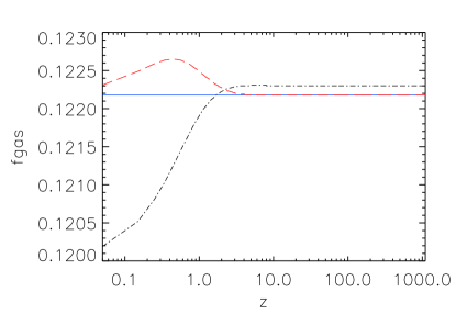
We therefore include in our analysis priors on systematic effects, and combine the simulated $f_{gas}$ data with mock CMB data of the Planck satellite. In fact, Planck is expected to measure the physical energy density of baryons and of dark matter to the subpercent level, as well as the angular diameter distance at redshift $1100$ with very high accuracy, thus providing information on a combination of $H_{0}$, $w_{0}$, $w_{a}$ and $\Omega_{k}$. These parameters are, however, completely degenerate with each other in CMB data. For this reason, $f_{gas}$ data, as well as other redshift-distance relation probes like Supernovae hutturn_optSN1 ; hutturn_optSN2 , are crucial for dark energy studies. As an example, Fig. 1 shows the evolution of $f_{gas}$ for different combinations of the true values of $H_{0}$, $w_{0}$ and $w_{a}$. The combinations are chosen to provide the same angular diameter distance at the redshift of recombination, i.e., to be completely degenerate in CMB data. Is is evident from this figure that the $f_{gas}$ data breaks this degeneracy.

Figure 1: Evolution of $f_{gas}$ with redshift for different values of the true cosmological parameters. The blue solid line shows the evolution for true cosmology parameters equal to the reference values, as reported in Tab. 1 and systematics as in Tab. 2. The dashed red line is for $w_{0}=-0.975$ and $w_{a}=-0.09$ in the true cosmology, while the dot-dashed is for $w_{0}=-0.975$ and $h_{0}=0.71$. Each of these three sets of parameters provide similar angular diameter distances at high redshifts.

II Fisher matrix Analysis

We expect the Planck cluster catalog to significantly increase the number of massive systems known at intermediate redshifts chamballu10 , and hence the number of suitable sources for $f_{gas}$ studies. The context guiding our present study is the possibility of observing $\sim 100$ clusters with XMM-Newton and Chandra from the newly-detected Planck clusters. We therefore aim to quantify the gain in cosmological constraints achievable with such a data set. To that end, we employ the Fisher Matrix methodology (see e.g., tegmark ). We will also study constraints from $f_{gas}$ measurements combined with the CMB anisotropy data expected from Planck.

For the cosmological parameters, we adopt the physical baryon and CDM densities, $\omega_{b}=\Omega_{b}h^{2}$ and $\omega_{c}=\Omega_{c}h^{2}$, the Hubble parameter $H_{0}$ and the parameters describing the dark energy equation-of-state (EoS). We consider a constant EoS, $w$, as well as an evolving EoS of the form $w_{\rm 0}$ and $w_{\rm a}$: $w(z)=w_{\rm 0}+(1-(1+z)^{-1})w_{\rm a}$. Furhermore, we examine both the cases of a flat universe and universes with free curvature $\Omega_{k}$.

When simultaneously fitting for $f_{gas}$ and CMB data, we add in addition the normalization, $A_{s}(k=0.002/Mpc)$, and scalar spectral index, $n_{s}$, of the primordial fluctuations, as well as the optical depth to reionization, $\tau$. As fiducial model for this parameter set, we use the best fit from the 5-year release of the WMAP satellite data (WMAP5) wmap5 , reported in Table 1. We verified that using the best fit from the 7-year release (WMAP7) wmap7 does not change any of our results. Finally, we also consider seven additional parameters to describe systematic effects as in Eq. 4 and Eq. 5, and listed in Table 2 with the assumed priors. The priors adopted are the same as in allen . They reflect the current knowledge of their magnitude and therefore are conservative expectations for future data. Since the Fisher analysis only allows Gaussian priors, for those parameters with a uniform prior, we choose to interpret half of the uniform intervals as the $2\sigma$ bounds of Gaussian priors. In section IV, we perform a MCMC analysis using the correct priors.

Parameter	Fiducial
$H_{0}$	$71.9$ Km/s/Mpc
$\Omega_{b}$	$0.02273$
$\Omega_{c}$	$0.1099$
$\Omega_{k}$	$0$
$w_{\rm 0}$	$-1$
$w_{\rm a}$	$0$
$\tau$	$0.089$
$n_{s}$	$0.963$
$A_{s}$	$2.41\times 10^{-9}$

Table 1: Fiducial WMAP5 marginalized cosmological parameters wmap5 .

For the $f_{gas}$ data, the Fisher Matrix is:

$$F^{\rm f_{gas}}_{ij}=\sum_{k=1}^{\rm N_{clusters}}\frac{\partial{\rm f_{gas}}(z_{k})}{\partial\theta_{i}}[\mathcal{C}_{kk}]^{-1}\frac{\partial{\rm f_{gas}}(z_{k})}{\partial\theta_{j}}$$ (10)

where the sum is over the number of clusters $N_{\rm clusters}$ and $\mathcal{C}$ is the covariance matrix of $f_{gas}$ . In our case, $\mathcal{C}$ is diagonal and equal to $\mathcal{C}=\sigma I$, with $\sigma=10\%\times{\rm f_{gas}}(z_{k})$, as the errors on the measured $f_{gas}$ at different redshifts are not correlated and we suppose that the errors are the same for all clusters.

Dividing the redshift range into $N_{bins}$, each containing $n_{bin}$ clusters, Equation 10 can be expressed as:

$$F^{\rm f_{gas}}_{ij}=\sum_{{bin}=1}^{N_{bins}}n_{bin}\frac{\partial{\rm f_{gas}}(z_{bin})}{\partial\theta_{i}}\frac{1}{\sigma^{2}}\frac{\partial{\rm f_{gas}}(z_{bin})}{\partial\theta_{j}}$$ (11)

This equation shows explicitly the dependence of the $f_{gas}$ Fisher Matrix on the redshift distribution of the clusters, i.e., the number $n_{bin}$ of clusters in each bin. This is what we want to optimize.

It is interesting to note that the tightest contraints on cosmological parameters do not necessarly follow from clusters at redshifts where the variation of $f_{gas}$ with the parameters, i.e., $\frac{\partial{\rm f_{gas}}(z_{bin})}{\partial\theta_{i}}$, is largest. In fact, degeneracies between parameters invalidate this deduction, making the optimal redshift distribution depend on the precision of the data and its degeneracy-breaking power, as well as on the influence of other (non $f_{gas}$ ) constraints.

Parameter
Calibration/Modeling	$K$	1.$\pm$ 0.10	Gaussian
Non-thermal pressure	$\gamma$	$0.9<1<1.1$	Uniform
Gas depletion	$b_{0}$	$0.66<0.83<1$	Uniform
$b(z)=b_{0}(1+\alpha_{\rm b}z)$	$\alpha_{\rm b}$	$-0.1<0.<0.1$	Uniform
Stellar mass	$s_{0}$	($0.162\pm 0.049)h_{70}^{0.5}$	Gaussian
$s(z)=s_{0}(1+\alpha_{\rm s}z)$	$\alpha_{\rm s}$	$0.2<0<0.2$	Uniform
Angular correction	$\eta$	$0.214\pm 0.022$	Gaussian

Table 2: Fiducial values and priors for systematic parameters in $f_{gas}$ . In the Fisher Matrix analysis, these priors are all considered as Gaussian priors. See text for references and details.

For the CMB data, the Fisher Matrix is:

$$F^{\rm CMB}_{ij}=\sum_{XY}\sum_{\ell}\frac{\partial{C}_{\ell}^{X}}{\partial\theta_{i}}[\mathcal{C}_{\ell}^{XY}]^{-1}\frac{\partial C_{\ell}^{Y}}{\partial\theta_{j}}$$ (12)

where $C^{X,Y}_{\ell}$ denotes the CMB angular power spectra X,Y=TT, EE, TE, plus the effective noise power spectrum of Equation 13 below, and $\mathcal{C}_{\ell}^{XY}$ is the covariance matrix of the $C^{X,Y}_{\ell}$ as defined in verde . We simulate angular power spectra using the camb codecamb adopting the expected values for the 143 GHz channel of the Planck satellite planck . The experimental noise on the angular power spectrum is described as in knox :

$$N_{\ell}=\left(\frac{w^{-1/2}}{\mu{\rm K\mbox{-}rad}}\right)^{2}\exp\left[\frac{\ell(\ell+1)(\theta_{\rm FWHM}/{\rm rad})^{2}}{8\ln 2}\right],$$ (13)

with $w^{-1}=3\times 10^{-4}\mu K^{2}$ as the temperature noise level (we consider a factor $\sqrt{2}$ larger for polarization noise) and $\theta_{\rm FWHM}=7^{\prime}$ for the beam size planck . We neglect the contribution of primordial B-mode polarization spectra and the lensing signal and we take $f_{sky}=1$ for the sky coverage. We however verified that assuming a smaller sky coverage, e.g. $f_{sky}=0.65$, lowers the FoM by less than $\lesssim 10\%$.

III Search for the Optimal distribution

We calculate the total Fisher Matrix to estimate the cosmological parameters by summing the CMB and $f_{gas}$  Fisher Matrices:

$$F^{\rm Tot}(n_{bin})=F^{\rm CMB}+F^{\rm f_{gas}}(n_{bin})$$

The number of clusters in each redshift bin $n_{bin}$ are the free parameters in our analysis. We search for the redshift distribution $n_{bin}$ that provides the highest value for the FoM , calculating the latter from the standard deviations $\sigma_{ii}=(F^{Tot})_{ii}^{-1}$ for each tested redshift distribution and using a maximization algorithm praxis .

We first optimize the cluster distribution for the case of linear evolution of the dark energy equation-of-state in a flat universe, i.e., when $w(z)=w_{\rm 0}+(1-(1+z)^{-1})w_{\rm a}$, constrained using a combination of CMB and $f_{gas}$ data. In Table 3, we report the optimal distribution for 100 clusters in 10 bins over the redshift range $z=0-1$. This maximizes the FoM to a value of $15.2$.

Redshift Interval	Number of clusters $n_{bin}$
0.0 - 0.1	38
0.1 - 0.2	0
0.2 - 0.3	0
0.3 - 0.4	45
0.4 - 0.5	0
0.5 - 0.6	0
0.6 - 0.7	0
0.7 - 0.8	0
0.8 - 0.9	0
0.9 - 1.0	17

Table 3: Optimal distribution for 100 clusters in the redshift range $z=0-1$ for the ($w_{0}-w_{a},\Omega_{k}=0$) model.

The distribution presents a peak in the first bin at the lowest redshift, a second peak at an intermediate redshift of $z\sim 0.35$ and then a third smaller peak in the last bin. This distribution improves the figure of merit by 30% compared to a simple uniform distribution, which has a FoM of 11.3.

The shape of this optimized distribution is determined by the various factors. The expected Planck CMB data provide excellent contraints on the single values of $\omega_{b}$ and $\omega_{c}$ at subpercent level. However, they can only constrain the combination of $H_{0}$, $w_{0}$, $w_{a}$ and $\Omega_{k}$ (but we are here first considering the case of a flat universe) because of the geometric degeneracy. Thus, the $f_{gas}$ distribution is optimized to break at best the degeneracy between these parameters, as well as the additional degeneracies introduced by the presence of $f_{gas}$ systematics.

Suppose, at first, that systematics are perfectly known. In this case, measuring the $f_{gas}$ at low redshift permits us to measure $H_{0}$, as the effect of $w_{0}$ and $w_{a}$ at these redshifts is negligible. This can be easily shown from Eq. 5, which in the limit of small $z$ becomes:

$$\lim_{z\to 0}f^{\rm ref}_{\rm gas}(z;\theta^{\rm ref}_{2500})=f^{\rm true}_{\rm gas}(z)\left[\frac{H_{0}^{\rm true}}{H_{0}^{\rm ref}}\right]^{1.5}$$ (14)

Thus, a measurement of $f_{gas}$ at the smallest possible redshift separates the effect of $H_{0}$ from $w_{0},w_{a}$, provided that $\omega_{b}$ and $\omega_{c}$ are sufficiently well measured by the CMB data.

Consider now the effect of redshift-independent systematics. They can change the value of the $f_{gas}$ at low redshifts, thus being degenerate with $H_{0}$. Measuring $f_{gas}$ at high redshifts can help disentangle these effects, given that the redshift-dependent systematic parameters are limited by priors. This explains why the optimal distribution places clusters in the highest redshift bin.

Finally, the central peak isolates the effects of $w_{0}$ and $w_{a}$. This peak is expected to be near to or at slightly higher redshift than the equivalence between dark energy and matter in the fiducial true cosmology, i.e., around $z_{eq}\sim 0.42$. At this redshift, the variation of $f_{gas}$ on true values of $w_{0}$ and $w_{a}$ differs from the reference ones is maximized, as also shown in Fig. 1.

There are two issues with this result. The first is that the optimal distribution in Tab. 3 peaks in a bin corresponding to redshifts smaller than $z=0.42$. This is due to systematic effects, as their uncertainties grow with redshift, so measurements at low $z$ can better constrain the parameters of interest. The second is the fact that we obviously do not know the true value of $z_{eq}$; however, recent data (see e.g. pandolfi ) show that the redshift of equivalence is between $0.35\lesssim z\lesssim 0.55$ at 68% c.l., in the case of a dark energy equation of state as considered here. We verified that even if the true $z_{eq}$ is different from the fiducial one, within the current constraints, the optimal distribution of Tab. 3 still provides a FOM that is very close (within $\sim 5\%$) to the maximum value.

Thus we conclude that the use of the optimal distribution of Tab. 3 provides a FOM very close to the maximum obtainable, even when the fiducial true cosmology is changed.

We also perform several tests to check the optimal distribution in a wide range of cases:

• We check the stability of the shape of the optimal distribution by testing that small changes in the distribution still provide high FoM values. We perform this test by finding the distributions that provide a FoM within 5% of the maximum value. These distributions are calculated by sampling the FoM on a regular grid of the $n_{bin}$ parameters, using a step of $\Delta n_{bin}=10$. This check confirms that all the distributions corresponding to a high value of the FoM are similar to the one in Table 3, i.e. have most of the clusters in the first, last and intermediate bin around $z\sim 0.42$.

  This is shown in Fig. 2, where we plot the optimal distributions for the $(w_{0},w_{a},\Omega_{k}=0)$ model, and the distributions with FoM within 5% of the maximum FoM obtainable with the optimal distribution.

  

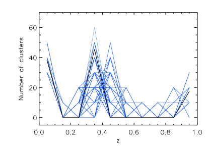
  Figure 2: The black thick line shows the optimal redshift distribution of galaxy clusters in 10 redshift bins in the range z=0-1, corresponding to the highest FoM =15.2 (from the Fisher Matrix analysis). The blue lines show the redshift distributions that have a FoM within 5% of the maximum value.

• We check that the optimal distribution has roughly the same behavior when different redshift ranges are considered, i.e., when the maximum redshift assumes a value between $z_{max}=0.9$ and $z_{max}=3$. This check has a purely theoretical interest for the higher redshifts, as it seems very unlikely that present and near-future experiments will detect many massive hot clusters at $z\gtrsim 1.5$. Nevertheless, we perform this analysis to better understand the shape of the optimal distributions. The optimal distributions appear to all have similar characteristics for different redshift ranges. Indeed, all of them have around $\sim 35\%$ of the clusters in the first bin, $\sim 15\%$ in the last, and almost all the remaining clusters in the intermediate bin close to $z_{eq}$. A minor peak ($\sim 5\%$ of the clusters) also appears at $z\sim 1.15$ when $z_{max}\gtrsim 1.8$.

  Fig. 3 shows the constraints on the dark energy parameters, as well as the FoM , for a ($w_{0}-w_{a},\Omega_{k}=0$) model, as a function of the maximum redshift $z_{max}$ of the redshift range $0-z_{max}$, for both the optimal and uniform distributions. It is interesting to note that the FoM obtained using a uniform distribution increases with the maximum redshift till $z_{max}=1.3$ and then starts decreasing again. The gain in FoM offered by pushing the observations of a uniform distribution to such a maximum redshift is, in any case, small as the FoM obtained is only 11.5.

  

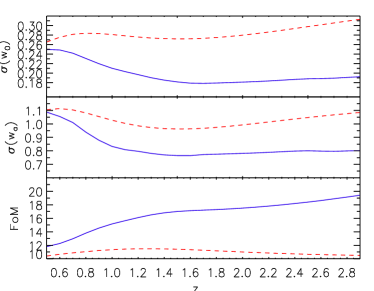
  Figure 3: FoM and the standard deviations of $w_{0}$ and $w_{a}$ as a function of the maximum redshift. We determine these constraints by combining simulated Planck CMB data and $f_{gas}$ measurements for $100$ clusters in the redshift range $0-z_{max}$. We show both the results for an optimal (blue solid lines) and a uniform (red dashed lines) distribution of clusters. These results are obtained with the Fisher Matrix analysis.

• We also verify that a very similar optimal distribution is obtained when instead of CMB data we consider priors of $\Omega_{b}h^{2}=0.0213\pm 0.002$ omeara and $H_{0}=73.8\pm 2.4$ riess11 in combination with the $f_{gas}$ data. In this case we find that the optimal distribution is almost the same as when using the full analysis with CMB+$f_{gas}$ . This is due to the fact that now the clusters in the low redshift bin are used to constrain $\omega_{c}$ instead of $H_{0}$, as also this parameter has a strong effect on the $f_{gas}$ at low $z$. For the $z=0-1$ range in the ($w_{0}-w_{a}$,$\Omega_{k}=0$) model, the maximum FoM achievable is only 3.9. This is due the absence of the high redshift measurement of the angular diameter distance provided by the CMB. In fact, while the effect of $w_{0}$ and $w_{a}$ on $f_{gas}$ , i.e., on the ratio of the angular diameter distances $d_{A}^{\rm ref}/d_{A}^{\rm true}$, decreases with redshift some time after the epoch of equality, their integrated effect on the overall true angular diameter distance at high redshift is conserved. This is useful to constrain $w_{a}$, which has a weak effect on $f_{gas}$ (compared for example to $w_{0}$). Thus, in absence of such a high redshift information, the FoM remains very small.

• We also study how much the systematics affect the optimal distribution and the FoM . The upper-left plot of Fig. 4 shows the optimal distribution of Tab. 3, obtained assuming priors on systematics as in Tab. 2, as well as the optimal distribution obtained assuming that systematic effects are perfectly known. In this last case, the last bin disappears, as the degeneracy between $H_{0}$ and the systematics is no longer present, while the intermediate peak of clusters shifts at the bin centered in $z=0.55$. The maximum FoM obtainable in this case is obviously much higher than in the case when systematic uncertainties are present, namely FoM $=51.5$. This indicates that the forecasted $f_{gas}$ data is not enough to break degeneracies between systematics and cosmological parameters. Thus, priors heavily affect the constraints on dark energy.

• We check that the optimal distribution in Tab. 3 for the ($w_{0}-w_{a},\Omega_{k}=0$) model provides high FoM also when other theoretical frameworks are tested. We consider in total 4 models:

  1. Linear redshift evolution of the dark energy equation of state in a flat universe ($w_{0}-w_{a},\Omega_{k}=0$). This is the model we used to obtain the optimal distribution in Tab 3.

  2. Linear redshift evolution of the dark energy equation of state with free curvature ($w_{0}-w_{a},\Omega_{k}$).

  3. Constant equation of state in a flat universe ($w_{0},w_{a}=0,\Omega_{k}=0$).

  4. Constant equation of state with free curvature ($w_{0},w_{a}=0,\Omega_{k}$).

  We find the optimal distribution for each of these models, as shown in Fig. 4. In the figure, we also show the optimal distribution one would obtain if all the systematics were perfectly known.

  

  

  

  

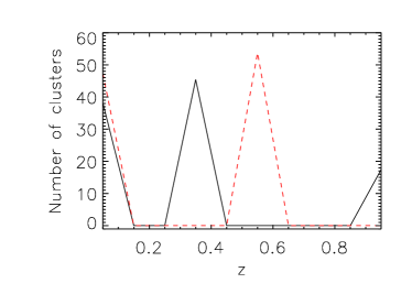
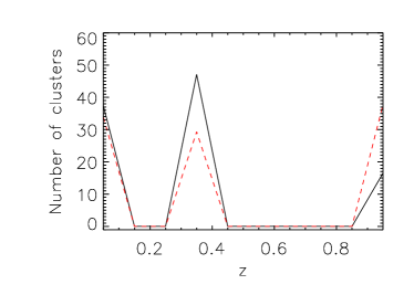
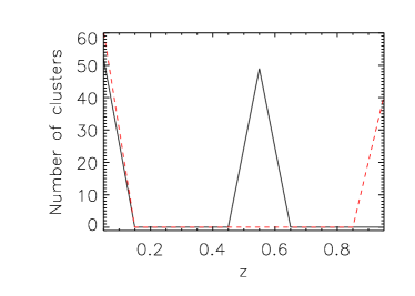
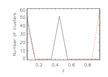
  Figure 4: Optimized distributions of clusters for the ($w_{0}$-$w_{a}$, $\Omega_{k}=0$) model (top-left), for ($w_{0}$-$w_{a}$, $\Omega_{k}$) (top-right), for ($w_{0},w_{a}=0,\Omega_{k}=0$) (bottom-left) and for ($w_{0}w_{a}=0,\Omega_{k}$) (bottom-right). We show the results for the case using priors on systematics as in Tab.2 (black solid lines) and assuming perfectly known systematics (red dashed lines).

  From the figure, it can be noticed that the distribution for the ($w_{0}-w_{a},\Omega_{k}$) model is very similar to the one obtained in the flat case. The reason is that now the last redshift bin is used to determine curvature, rather than systematic effects. In this way, however, systematics are constrained only by the priors, lowering the possible FoM achievable, which is ${\rm FoM}=10.2$.

  Considering now the case of a constant equation of state in a flat universe, $(w_{0},w_{a}=0,\Omega_{k}=0)$, we find the optimal distribution by minimizing the standard deviation of $w_{0}$. In this case the optimal distribution presents only two peaks. Roughly half of the clusters are in the first bin, in order to determine the Hubble constant. The rest of the clusters are placed in an intermediate bin at $z=0.55$, where the effect of systematics is better disantagled from the effect of $H_{0}$. In fact, the uncertainty on the systematics grows with $z$, due to the redshift dependence of the stellar mass $a_{s}$ and of the depletion factor $\alpha_{b}$. However, $H_{0}$, measured at low redshift, is mostly degenerate with all those systematic effects that are redshift independent, namely the combination of $K$, $\gamma$, $b_{0}$, and $s_{0}$. Thus, it is convenient to measure these systematics where the redshift-dependent effects are still subdominant, at redshift lower than 1. If we now consider the case where systematics are perfectly known, the peak at intermediate redshift disappears, while some clusters are placed in the last bin. This is due to the fact that measurements at this redshift can now improve the error bars obtained from the CMB on $\omega_{c}$ and $\omega_{b}$, and thus further decrease the degeneracy that these parameters have with the Hubble parameter at low redshifts in $f_{gas}$ data.

  Finally, we consider the case of a constant equation-of-state with free curvature, $(w_{0},w_{a}=0,,\Omega_{k})$. The optimal distribution found is similar to the one for the flat case.

  We then compare the FoM and $\sigma(w_{0})$ obtained with the optimal distributions in the different frameworks, with the constraints obtained using the optimal distribution of Tab. 3 in the three other frameworks. The results are showed in Tab.4. It is evident from the table that using the optimal distribution of Tab. 3 also in these other cases leads to FoM which are very close to the ones obtainable by using the proper optimal distribution for each case. For example, for the $(w_{0},w_{a}=0,\Omega_{k}=0)$ model, the error obtained on $w_{0}$ using the proper optimal distribution is $\sigma(w_{0})=0.073$, while the one obtained using the optimal distribution of Tab. 3 yields to $\sigma(w_{0})=0.079$; the variation is less than $\sim 10$%. Thus we conclude that the distribution in Tab. 3 can be used in a wide range of models to obtain tight constraints on the dark energy equation-of-state.

  Model	FoM
  	Uniform	Optimal		TAB. 3
  		Syst.	No syst.
  $w_{0}-w_{a},\Omega_{k}=0$	11.3	15.2	51.5	.
  $w_{0}-w_{a},\Omega_{k}$	7.7	10.3	18.1	10.3
  Model	$\sigma(w_{0})$
  	Uniform	Optimal		TAB. 3
  		Syst.	No syst.
  $w_{0},\Omega_{k}=0$	0.086	0.073	0.035	0.079
  $w_{0},\Omega_{k}$	0.11	0.098	0.048	0.10

  Table 4: Constraints on FoM (or $\sigma(w)$ in the case of a constant dark energy equation of state) obtained by combining Planck CMB data and the $f_{gas}$ data for 100 clusters with different distributions. We show the results using a uniform distribution, an optimal distribution calculated in each of the models considered and using the optimal distribution found for the ($w_{0}-w_{a},\Omega_{k}=0$) case reported in Tab. 3. For the second distribution considered, we also report the results obtainable in the case of perfectly known systematic effects (’No syst.’).

IV MCMC analysis

IV.1 Method

In order to check our previous results obtained using Fisher matrix forecasts, we derive the constraints on cosmological parameters using a modified version of the publicly available Markov Chain Monte Carlo package cosmomc Lewis:2002ah . We use a convergence diagnostics based on the Gelman and Rubin statistic performed on $4$ chains, and the Parameterized Post-Friedmann(PPF) prescription for the dark energy perturbations husawicki implemented by fang in the camb code. Moreover, we use the code of rapetticode to implement the $f_{gas}$ data in the cosmomc code.

We simulate datasets for the Planck experiment following the commonly used approach, described, for example, in perotto . We first generate the fiducial theoretical angular power spectra $C_{\ell}^{TT}$, $C_{\ell}^{TE}$, $C_{\ell}^{EE}$ with the camb code for a cosmological model compatible with the WMAP5 maximum likelihood parameters reported in Table 1. We then add the experimental noise $N_{\ell}$ described in Equation 13.

For $f_{gas}$ we simulate a dataset of 100 clusters over the redshift range $z=0-1$, distributed with either the optimal configuration reported in Table 3 or with a uniform distribution. We assume that the true and the reference cosmology are the same as the fiducial model of Table 1. A 10% error is assigned to the measurements.

We sample a set of cosmological parameters similar to the one used in the Fisher Matrix analysis, adopting flat priors: the physical baryon and cold dark matter densities, $\omega_{b}=\Omega_{b}h^{2}$ and $\omega_{c}=\Omega_{c}h^{2}$, the ratio of the sound horizon to the angular diameter distance at decoupling, $\theta_{S}$ (used instead of $H_{0}$), and the curvature $\Omega_{k}$. For the CMB data, we additionally consider the scalar spectral index $n_{S}$, the overall normalization of the spectrum $A$ at $k=0.002$ Mpc^-1, and the optical depth to reionization, $\tau$. Furthermore, for $f_{gas}$ we consider the seven systematic parameters described in Section 4, with the priors in Table 2.

We test the four models considered in the Fisher Matrix analysis, i.e., a linear evolution of the dark energy equation of state $w_{0}-w_{a}$ in a flat and non-flat universe, and a constant value of the dark energy equation-of-state $w_{0}$ in a flat and non-flat universe.

IV.2 Results

Table 5 shows our constraints on the most interesting varied and derived parameters for all the models and combinations of data tested, obtained using the cosmomc code. Concerning the $(w_{0}-w_{a},\Omega_{k}=0)$ model, the FoM found with a combination of the synthetic Planck CMB data plus an optimal distribution of $f_{gas}$ data is smaller than the Fisher Matrix value in Table 4 ($14.4$, instead of $15.1$) due to better accounting of uniform priors and a more reliable treatment of the non-Gaussian probability distributions of the parameters. Nevertheless, the combination of Planck CMB+$f_{gas}$ data with an optimal distribution still improves the FoM by $\sim 26\%$ compared to a uniform distribution over the same redshift range, which provides a FoM of 11.4.

Data	$\sigma(w_{0})$	$\sigma(w_{a})$	$\sigma(\Omega_{de})$	$\sigma(\Omega_{m})$	$\sigma(H_{0})$	$\sigma(\Omega_{K})$	FOM
Model: $w_{0}-w_{a},\Omega_{k}=0$
WMAP5+Allen $f_{gas}$	0.28	0.97	0.035	0.035	4.3	.	8.3
Planck+$f_{gas}$ (opt.)	0.20	0.75	0.028	0.028	3.5	.	14.5
Planck+$f_{gas}$ (uni.)	0.25	0.88	0.028	0.028	3.7	.	11.4
Planck+ Allen $f_{gas}$	0.28	1.0	0.029	0.029	4.1	.	8.8
Planck+	0.17	0.54	0.024	0.024	3.0	.	24.2
+$f_{gas}$ [Allen + (opt.)]
Model: $w_{0}-w_{a},\Omega_{k}$
Planck+$f_{gas}$ (opt.)	0.20	0.94	0.031	0.040	4.6	0.016	7.5
Planck+$f_{gas}$ (uni.)	0.26	1.0	0.032	0.041	4.7	0.014	6.1
Model: $w_{0},w_{a}=0,\Omega_{k}=0$
Planck+$f_{gas}$ (opt.)	0.091	.	0.026	0.026	3.3	.	.
Planck+$f_{gas}$ (uni.)	0.098	.	0.028	0.028	3.5	.	.
Model: $w_{0},w_{a}=0,\Omega_{k}$
Planck+$f_{gas}$ (opt.)	0.14	.	0.030	0.039	4.6	0.013	.

Table 5: Figures of merit and 68% c.l. errors on cosmological parameters for different models, obtained using the cosmomc code. The dark energy and dark matter density parameters $\Omega_{de}$ and $\Omega_{m}$ are indirectly derived. We show the results for different combinations of data. ‘WMAP5’ indicates CMB data from the 5-year release of the WMAP satellite data wmap5 , while ‘Planck’ indicates simulated CMB data from the Planck satellite planck . ‘$f_{gas}$ (opt).’ indicates $f_{gas}$ simualated data for $100$ clusters with an optimal distribution between redshift $0$ and $1$, while ’$f_{gas}$ (uni.)’ is for a uniform distribution. Finally, ‘Allen’ indicates $f_{gas}$ real data for 42 clusters publicated in Allen et al. allen .

Moreover, the results obtained with the combination of synthetic Planck CMB+optimal $f_{gas}$ represent a major improvement over current data. For instance, we calculated the FoM from WMAP5 CMB combined with the $f_{gas}$ data for $42$ clusters measured by Allen et al.allen . These datasets yield a FoM of 8.3; therefore, future data will improve this result by almost a factor $\sim 2$, as clear from the second line of Tab. 5. An even more impressive improvement is obtained if in addition to the synthetic Planck CMB data and the $f_{gas}$ data for 100 clusters with an optimal distribution, we add the known 42 $f_{gas}$ measurements of Allen et al. In this case the FoM will increase of almost a factor $3$.

The results in Table 5 also demonstrate that the improvement in the determination of the dark energy equation-of-state will be mainly driven by more accurate $f_{gas}$ data rather than better CMB data. In fact, combining Planck CMB data with Allen et al.’s $f_{gas}$ measurements only provides a FoM slightly better than that the one obtained with WMAP5 data — nominally FoM =8.8.

Fig. 5 shows the 68% and 95% likelihood contour plots in the $w_{0}$ - $w_{a}$ plane, obtained using current data and synthetic Planck CMB plus $f_{gas}$ data for the 42 clusters reported in Allen et al.allen plus $f_{gas}$ forecasted data with an optimal cluster distribution. Fig. 6 compares the constraints achievable by Planck CMB only and Planck CMB+$f_{gas}$ forecasted data for 100 clusters with an optimal distribution.

Figure 5: 68% and 95% likelihood contour plots on the $w_{0}$ - $w_{a}$ plane for WMAP5 plus $f_{gas}$ data for the 42 clusters reported in Allen et al. allen (red) and synthetic Planck plus $f_{gas}$ data for the 42 clusters reported in Allen et al.allen , plus $f_{gas}$ data for 100 clusters between redshift 0 and 1 with an the optimal distribution (yellow). Here the model considered is $(w_{0}-w_{a},\Omega_{k}=0)$ in a flat universe.

Figure 6: Constraints for the $(w_{0}-w_{a},\Omega_{k}=0)$ model from synthetic Planck CMB data (red) and CMB+ $f_{gas}$ data (blue) for 100 clusters with an optimal distribution between $z=0-1$. We show the marginalized one-dimensional distributions and two-dimensional 68% and 95% c.l. contour plots.

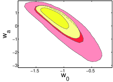
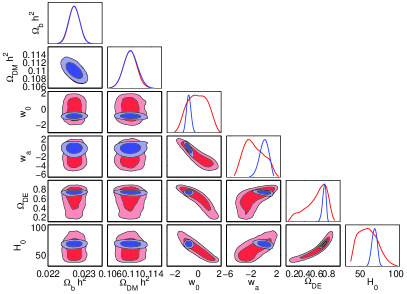
In this plot, the degeneracy-breaking power of the $f_{gas}$ data on the parameters that determine the geometry of the universe, such as the dark energy equation of state parameters $w_{0}$, $w_{a}$ and the Hubble constant, is striking. By themselves, CMB data can only place weak constraints on these parameters when they are considered simultaneously. As expected, adding $f_{gas}$ data to CMB data do not improve the constraints on other parameters, namely the baryon and dark matter densities $\omega_{b}$ and $\omega_{c}$, the spectral index $n_{s}$, and the optical depth $\tau$.

Very similar considerations can be made for a constant equation of state $w=w_{0}$ in a flat universe ($\Omega_{k}=0$), as show in Figure 7.

Figure 7: Constraints for the $(w_{0},w_{a}=0,\Omega_{k}=0)$ model from synthetic Planck CMB data (red) and CMB+ $f_{gas}$ data (blue) for 100 clusters with an optimal distribution between $z=0-1$. We show the marginalized one-dimensional distributions and two-dimensional 68% and 95% c.l. contour plots.

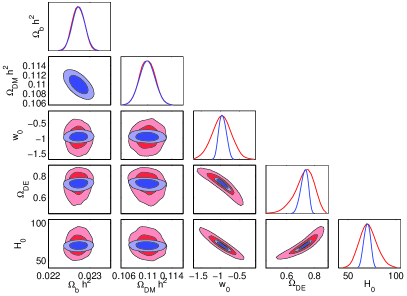
In this case, the constraint on $w_{0}$ is $\sigma(w_{0})=0.091$, which represents a $35\%$ improvement compared to the results reported in Allen et al. using WMAP3 CMB data and 42 clusters, namely $\sigma(w_{0})=0.14$.

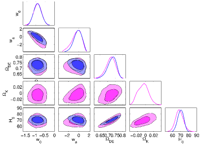
Finally we repeated the analysis for also the case of a universe with free curvature. Fig. 8 shows the constraints obtained for the $(w_{0}-w_{a},\Omega_{k})$ model. The main effect of adding free curvature is to introduce more degeneracy with the parameters of interest. This leads to a widening of the errors and a distortion of the probability distributions. This also explains why the FoM obtained with the MCMC analysis in $(w_{0}-w_{a},\Omega_{k})$ case, FoM =$7.5$, is 30% smaller than the one estimated with the Fisher Matrix, FoM =10.3, that assumes Gaussian likelihoods for the considered parameters.

Figure 8: Constraints for the $(w_{0}-w_{a},\Omega_{k})$ model from synthetic Planck CMB data + $f_{gas}$ data (magenta) for 100 clusters with an optimal distribution between $z=0-1$, compared to constraints for a flat universe (blue). We show the marginalized one-dimensional distributions and two-dimensional 68% and 95% c.l. contour plots.

V Conclusions

We consider constraints on the dark energy equation-of-state obtained when combining the future CMB data expected from the Planck satellite and simulated $f_{gas}$ measurements for 100 clusters observed by a possible future X-ray campaign with X-ray satellites. We found the optimal cluster distribution over the redshift range $z=0-1$ to provide the tightest constraints on the dark energy equation-of-state. The optimal distribution improves the FoM by almost $\sim 30\%$ compared to a uniform distribution. We found that the optimal distribution, found for a linearly evolving dark energy equation of state in a flat universe, provides very high figures of merit also in other theoretical frameworks, namely free curvature or a constant equation-of-state. A positive characteristic of the optimal distribution is that clusters are placed at low and intermediate redshifts, while only a few should be observed at high redshift, where measurements require longer observational times. We performed our analysis by both using the Fisher Matrix and the MCMC methods to forecast constraints. We found that future data will increase the FoM by a factor $\sim 2$ relative to the current constraints available with WMAP5 and the $f_{gas}$ data from allen . Our study provides a useful guide for planning XMM-Newton and Chandra follow-up observations of Planck and SPT clusters.