Optimal growth for linear processes with affine control

Vincent Calvez Ecole Normale Supérieure de Lyon, UMR CNRS 5669 ’UMPA’, and Inria Rhône-Alpes, projet NUMED, 46 allée d’Italie, F-69364 Lyon cedex 07, France. Email: vincent.calvez@ens-lyon.fr    Pierre Gabriel Inria Rhône-Alpes, équipe-projet BEAGLE, BP 52132, 66 Boulevard Niels Bohr, F-69603 Villeurbanne cedex, France. Email: pierre.gabriel@inria.frCorresponding author
Abstract

We analyse an optimal control with the following features: the dynamical system is linear, and the dependence upon the control parameter is affine. More precisely we consider x˙α(t)=(G+α(t)F)xα(t)subscript˙𝑥𝛼𝑡𝐺𝛼𝑡𝐹subscript𝑥𝛼𝑡\dot{x}_{\alpha}(t)=(G+\alpha(t)F)x_{\alpha}(t), where G𝐺G and F𝐹F are 3×3333\times 3 matrices with some prescribed structure. In the case of constant control α(t)α𝛼𝑡𝛼\alpha(t)\equiv\alpha, we show the existence of an optimal Perron eigenvalue with respect to varying α𝛼\alpha under some assumptions. Next we investigate the Floquet eigenvalue problem associated to time-periodic controls α(t)𝛼𝑡\alpha(t). Finally we prove the existence of an eigenvalue (in the generalized sense) for the optimal control problem. The proof is based on the results by [Arisawa 1998, Ann. Institut Henri Poincaré] concerning the ergodic problem for Hamilton-Jacobi equations. We discuss the relations between the three eigenvalues. Surprisingly enough, the three eigenvalues appear to be numerically the same.

Keywords. Optimal control; Infinite horizon; Hamilton-Jacobi equation; Ergodic problem; Non coercive hamiltonian

1 Introduction

We aim at optimally controlling the following 3-dimensional system in the long-time horizon,

{x˙α(t)=(G+α(t)F)xα(t),xα(0)=x(+)3{0},casessubscript˙𝑥𝛼𝑡𝐺𝛼𝑡𝐹subscript𝑥𝛼𝑡subscript𝑥𝛼0𝑥superscriptsubscript30\left\{\begin{array}[]{l}\dot{x}_{\alpha}(t)=(G+\alpha(t)F)\,x_{\alpha}(t)\,,\vspace{1mm}\\ x_{\alpha}(0)=x\in\left(\mathbb{R}_{+}\right)^{3}\setminus\{0\}\,,\end{array}\right. (1.1)

where G,F3()𝐺𝐹subscript3G,F\in\mathcal{M}_{3}({\mathbb{R}}) are matrices with nonnegative off-diagonal entries, and α:++:𝛼subscriptsubscript\alpha:\mathbb{R}_{+}\to\mathbb{R}_{+} is a nonnegative control parameter. There is no running reward. Let T>0𝑇0T>0 be the final time. The final reward is the linear function m,xα(T)𝑚subscript𝑥𝛼𝑇\left\langle m,x_{\alpha}(T)\right\rangle, where m(+)3{0}𝑚superscriptsubscript30m\in\left(\mathbb{R}_{+}\right)^{3}\setminus\{0\} is in the kernel of FTsuperscript𝐹𝑇F^{T}: mTF=0superscript𝑚𝑇𝐹0m^{T}F=0.

We investigate the asymptotic behaviour of the optimal reward when T+𝑇T\to+\infty in the three different regimes: α𝛼\alpha is constant (constant control), α𝛼\alpha is periodic (periodic control), and α𝛼\alpha is any measurable function from (0,T)0𝑇(0,T) to [a,A]𝑎𝐴[a,A], where a,A𝑎𝐴a,A are given bounds (optimal control).

Because of the linear structure of system (1.1), we expect an exponential growth of the final reward. This motivates the introduction of the following renormalized reward:

rα(T,x)=1Tlogm,xα(T).subscript𝑟𝛼𝑇𝑥1𝑇𝑚subscript𝑥𝛼𝑇r_{\alpha}(T,x)=\frac{1}{T}\log\langle m,x_{\alpha}(T)\rangle\,.

When α𝛼\alpha is a constant (resp. periodic) control, it is well-known that rα(T,x)subscript𝑟𝛼𝑇𝑥r_{\alpha}(T,x) converges to the Perron (resp. Floquet) eigenvalue λP(α)subscript𝜆𝑃𝛼\lambda_{P}(\alpha) (resp. λF(α)subscript𝜆𝐹𝛼\lambda_{F}(\alpha)) of system (1.1) as T+𝑇T\to+\infty. Hence, the best control is obtained by optimizing the Perron (resp. Floquet) eigenvalue. In the case of optimal control, we define the best possible reward as follows,

V(T,x)=supα{m,xα(T):x˙α(t)=(G+α(t)F)xα(t),xα(0)=x},𝑉𝑇𝑥subscriptsupremum𝛼conditional-set𝑚subscript𝑥𝛼𝑇formulae-sequencesubscript˙𝑥𝛼𝑡𝐺𝛼𝑡𝐹subscript𝑥𝛼𝑡subscript𝑥𝛼0𝑥V(T,x)=\sup_{\alpha}\left\{\left\langle m,x_{\alpha}(T)\right\rangle\;:\;\dot{x}_{\alpha}(t)=(G+\alpha(t)F)x_{\alpha}(t)\;,\;x_{\alpha}(0)=x\right\}\,,

where the supremum is taken over all measurable control functions α:(0,T)[a,A]:𝛼0𝑇𝑎𝐴\alpha:(0,T)\to[a,A]. We can resolve this optimal control problem using the dynamic programming principle. This yields a Hamilton-Jacobi equation for the value function

v(s,x)=sup{m,xα(T):x˙α(t)=(G+α(t)F)xα(t),xα(s)=x},𝑣𝑠𝑥supremumconditional-set𝑚subscript𝑥𝛼𝑇formulae-sequencesubscript˙𝑥𝛼𝑡𝐺𝛼𝑡𝐹subscript𝑥𝛼𝑡subscript𝑥𝛼𝑠𝑥v(s,x)=\sup\left\{\left\langle m,x_{\alpha}(T)\right\rangle\;:\;\dot{x}_{\alpha}(t)=(G+\alpha(t)F)x_{\alpha}(t)\;,\;x_{\alpha}(s)=x\right\}\,,

defined for intermediate times 0<s<T0𝑠𝑇0<s<T. Namely it is solution to the following Hamilton-Jacobi-Bellman equation in the sense of viscosity solutions [5],

sv(s,x)+H~(x,Dxv(s,x))=0,𝑠𝑣𝑠𝑥~𝐻𝑥subscript𝐷𝑥𝑣𝑠𝑥0\frac{\partial}{\partial s}v(s,x)+\widetilde{H}(x,D_{x}v(s,x))=0\,,

where the Hamiltonian is given by H~(x,p)=maxα[a,A]{(G+αF)x,p}~𝐻𝑥𝑝subscript𝛼𝑎𝐴𝐺𝛼𝐹𝑥𝑝\widetilde{H}(x,p)=\max_{\alpha\in[a,A]}\left\{\left\langle(G+\alpha F)x,p\right\rangle\right\} (see Section 3 for details).

Under some assumptions we prove the following ergodic result: there exists a constant λHJsubscript𝜆𝐻𝐽\lambda_{HJ} such that,

x(+)3{0}limT+1TlogV(T,x)=λHJ.formulae-sequencefor-all𝑥superscriptsubscript30subscript𝑇1𝑇𝑉𝑇𝑥subscript𝜆𝐻𝐽\forall x\in\left(\mathbb{R}_{+}\right)^{3}\setminus\{0\}\,\quad\lim_{T\to+\infty}\dfrac{1}{T}\log V(T,x)=\lambda_{HJ}\,. (1.2)

This constant λHJsubscript𝜆𝐻𝐽\lambda_{HJ} is the analog of the Perron and Floquet eigenvalues in the case of optimal control. We have obviously,

supαλP(α)supαλF(α)λHJ.subscriptsupremum𝛼subscript𝜆𝑃𝛼subscriptsupremum𝛼subscript𝜆𝐹𝛼subscript𝜆𝐻𝐽\sup_{\alpha}\lambda_{P}(\alpha)\leq\sup_{\alpha}\lambda_{F}(\alpha)\leq\lambda_{HJ}\,.

Interestingly, numerical simulations show that these three eigenvalues may coincide (see Section 4 for a discussion).

Motivations and running example

From a theoretical viewpoint, the convergence result (1.2) is known as the ergodic problem for Hamilton-Jacobi equations. It appears in homogenization problems [22]. In this case the constant λ𝜆\lambda is called the effective hamiltonian [7, 16]. It can be interpreted as a nonlinear Perron eigenproblem associated with an eigenvector u¯¯𝑢\overline{u} which solves the following stationary Hamilton-Jacobi equation in the viscosity sense,

λ+H(y,Dyu¯)=0,yYformulae-sequence𝜆𝐻𝑦subscript𝐷𝑦¯𝑢0𝑦𝑌-\lambda+H(y,D_{y}\overline{u})=0\,,\quad y\in Y (1.3)

where H:Y×n+:𝐻𝑌superscript𝑛subscriptH:Y\times\mathbb{R}^{n}\to\mathbb{R}_{+} denotes the hamiltonian. It also appears in weak KAM theory for lagrangian dynamical systems [17, 18]. A natural way to attack this issue is to consider the following stationary Hamilton-Jacobi equation with small parameter ϵ>0italic-ϵ0\epsilon>0,

ϵuϵ+H(x,Dxuϵ)=0.italic-ϵsubscript𝑢italic-ϵ𝐻𝑥subscript𝐷𝑥subscript𝑢italic-ϵ0-\epsilon u_{\epsilon}+H(x,D_{x}u_{\epsilon})=0\,.

The asymptotic behaviour of uϵsubscript𝑢italic-ϵu_{\epsilon}, as ϵ0italic-ϵ0\epsilon\to 0, has been investigated in several works [22, 12, 17, 25, 9, 8, 21, 6, 1, 13]. In many cases the set Y𝑌Y is assumed to be compact, and the Hamiltonian H(y,p)𝐻𝑦𝑝H(y,p) is assumed to be coercive: H(,p)+𝐻𝑝H(\cdot,p)\to+\infty as |p|+𝑝|p|\to+\infty. Under these assumptions it can be proven that the function ϵuϵitalic-ϵsubscript𝑢italic-ϵ\epsilon u_{\epsilon} converges to a constant λ𝜆\lambda (uniquely determined) [22, 12, 17]. Moreover the function uϵsubscript𝑢italic-ϵu_{\epsilon} converges uniformly, up to extraction, to some lipschitz function u¯¯𝑢\overline{u}, solution of (1.3). However the function u¯¯𝑢\overline{u} is generally not unique. The question of convergence of uϵsubscript𝑢italic-ϵu_{\epsilon} towards u¯¯𝑢\overline{u} (modulo a large constant) has been investigated in [25, 9, 8].

In the context of optimal control, the coercivity of the hamiltonian H(y,p)=maxα𝒜{b(y,α),p}𝐻𝑦𝑝subscript𝛼𝒜𝑏𝑦𝛼𝑝H(y,p)=\max_{\alpha\in\mathcal{A}}\{\left\langle b(y,\alpha),p\right\rangle\} is guaranteed under the hypothesis of uniform controllability [12, 5]: there exists a constant μ>0𝜇0\mu>0 such that

yY¯B(0,μ)convexhull¯{b(y,α)|α𝒜}.formulae-sequencefor-all𝑦¯𝑌𝐵0𝜇¯convexhullconditional-set𝑏𝑦𝛼𝛼𝒜\forall y\in\overline{Y}\quad B(0,\mu)\subset\overline{\mathrm{convex\;hull}}\{b(y,\alpha)\;|\;\alpha\in\mathcal{A}\}\,.

This hypothesis ensures that any two points y,yY𝑦superscript𝑦𝑌y,y^{\prime}\in Y can be connected with some control α(t)𝛼𝑡\alpha(t) within a time T=O(|yy|)𝑇𝑂𝑦superscript𝑦T=O(|y-y^{\prime}|). This yields equicontinuity of the family (uϵ)ϵ>0subscriptsubscript𝑢italic-ϵitalic-ϵ0(u_{\epsilon})_{\epsilon>0}, and thus compactness.

The criterion of uniform controllability is not verified in our case, hence the hamiltonian is not coercive (see Remark 3.1 below). Different approaches have been developped to circumvent the lack of coercivity. Several works rely on some partial coercivity [21, 6, 1]. In [4] the authors introduce a non-resonance condition which yields ergodicity. This condition is restricted to hamiltonian with separated variables H(y,p)=H(p)+V(y)𝐻𝑦𝑝𝐻𝑝𝑉𝑦H(y,p)=H(p)+V(y). In [13] the author extends this result to the case of a non-convex hamiltonian H(p)𝐻𝑝H(p), in two dimensions of space. In the context of optimal control, Arisawa [2, 3] has shown the equivalence between ergodicity and the existence of a stable subset ZY𝑍𝑌Z\subset Y which attracts the trajectories. It is required in addition that the restriction of the system to Z𝑍Z is controllable. The present work follows the latter approach.

From a modeling viewpoint, this work is motivated by the optimization of some experimental protocol for polymer amplification, called Protein Misfolding Cyclic Amplification (PMCA) [26]. In the system (1.1) the matrix G𝐺G represents the growth of polymers in size, whereas F𝐹F is the fragmentation of polymers into smaller pieces. The vector m𝑚m encodes the size of the polymers. We restrict to dimension 3 for the sake of simplicity, i.e. three possible sizes for the polymers (small, intermediate, large). The orthogonality relation mTF=0superscript𝑚𝑇𝐹0m^{T}F=0 accounts for the conservation of the total size of polymers by fragmentation.

We now give a class of matrices which will serve as an example all along the paper. It is a simplification of the discrete growth-fragmentation process introduced in [23] to model Prion proliferation. We make the following choice:

G=(τ100τ1τ200τ20)andF=(02β2β30β2β300β3).formulae-sequence𝐺subscript𝜏100subscript𝜏1subscript𝜏200subscript𝜏20and𝐹02subscript𝛽2subscript𝛽30subscript𝛽2subscript𝛽300subscript𝛽3G=\left(\begin{array}[]{ccc}-\tau_{1}&0&0\\ \tau_{1}&-\tau_{2}&0\\ 0&\tau_{2}&0\end{array}\right)\qquad\text{and}\qquad F=\left(\begin{array}[]{ccc}0&2\beta_{2}&\beta_{3}\\ 0&-\beta_{2}&\beta_{3}\\ 0&0&-\beta_{3}\end{array}\right). (1.4)

Here τ1>0subscript𝜏10\tau_{1}>0 denotes the rate of increase from small to intermediate polymers, and τ2>0subscript𝜏20\tau_{2}>0 from intermediate to large polymers. The βi>0subscript𝛽𝑖0\beta_{i}>0 denote the fragmentation rates which distribute larger polymers into smaller compartments, keeping the total size constant. The size vector is m=(1 2 3)T𝑚superscript123𝑇m=(1\;2\;3)^{T}. Finally, the rate α(t)𝛼𝑡\alpha(t) accounts for sonication, i.e. externally driven intensity of fragmentation.

The continuous version of the baby model (1.1)-(1.4) consists in the following size-structured PDE with variable coefficients [20, 11, 15]

tf(t,ξ)+ξ(τ(ξ)f(t,ξ))=α(t)(2ξβ(ζ)κ(ξ,ζ)f(t,ζ)𝑑ζβ(ξ)f(t,ξ)).subscript𝑡𝑓𝑡𝜉subscript𝜉𝜏𝜉𝑓𝑡𝜉𝛼𝑡2superscriptsubscript𝜉𝛽𝜁𝜅𝜉𝜁𝑓𝑡𝜁differential-d𝜁𝛽𝜉𝑓𝑡𝜉\partial_{t}f(t,\xi)+\partial_{\xi}(\tau(\xi)f(t,\xi))=\alpha(t)\left(2\int_{\xi}^{\infty}\beta(\zeta)\kappa(\xi,\zeta)f(t,\zeta)\,d\zeta-\beta(\xi)f(t,\xi)\right)\,. (1.5)

Here, f(t,ξ)𝑓𝑡𝜉f(t,\xi) represents the density of protein polymers of size ξ>0𝜉0\xi>0 at time t𝑡t. The transport term accounts for the growth of polymers in size, whereas the r.h.s is the fragmentation operator. The final reward is the total mass of polymers, namely 0ξu(T,ξ)𝑑ξsuperscriptsubscript0𝜉𝑢𝑇𝜉differential-d𝜉\int_{0}^{\infty}\xi u(T,\xi)\,d\xi (see [19] for more details). The Perron eigenvalue problem for (1.5) has been investigated in [15, 10].

Main assumptions

(H1)

We assume that the matrices G𝐺G and F𝐹F are both reducible. We assume that the matrix G+αF𝐺𝛼𝐹G+\alpha F is irreducible for all α>0𝛼0\alpha>0.

From the Perron-Frobenius Theorem there exists a simple dominant eigenvalue λP(α)subscript𝜆𝑃𝛼\lambda_{P}(\alpha) and a positive left- (resp. right-) eigenvector eαsubscript𝑒𝛼e_{\alpha} (resp. ϕαsubscriptitalic-ϕ𝛼\phi_{\alpha}) such that:

{(G+αF)eα=λP(α)eα,eα>0,ϕαT(G+αF)=λP(α)ϕαT,ϕα>0.casesformulae-sequence𝐺𝛼𝐹subscript𝑒𝛼subscript𝜆𝑃𝛼subscript𝑒𝛼subscript𝑒𝛼0formulae-sequencesuperscriptsubscriptitalic-ϕ𝛼𝑇𝐺𝛼𝐹subscript𝜆𝑃𝛼superscriptsubscriptitalic-ϕ𝛼𝑇subscriptitalic-ϕ𝛼0\left\{\begin{array}[]{l}(G+\alpha F)e_{\alpha}=\lambda_{P}(\alpha)e_{\alpha},\quad e_{\alpha}>0\,,\vskip 6.0pt plus 2.0pt minus 2.0pt\\ \phi_{\alpha}^{T}(G+\alpha F)=\lambda_{P}(\alpha)\phi_{\alpha}^{T},\quad\phi_{\alpha}>0\,.\end{array}\right. (1.6)

We choose the following normalizations:

m,eα=1,ϕα,eα=1.formulae-sequence𝑚subscript𝑒𝛼1subscriptitalic-ϕ𝛼subscript𝑒𝛼1\left\langle m,e_{\alpha}\right\rangle=1\,,\quad\left\langle\phi_{\alpha},e_{\alpha}\right\rangle=1\,.

We denote by (λ1(α),λ2(α),λ3(α))subscript𝜆1𝛼subscript𝜆2𝛼subscript𝜆3𝛼(\lambda_{1}(\alpha),\lambda_{2}(\alpha),\lambda_{3}(\alpha)) the eigenvalues of the matrix G+αF𝐺𝛼𝐹G+\alpha F, where λ1(α)subscript𝜆1𝛼\lambda_{1}(\alpha)\in{\mathbb{R}} is the dominant eigenvalue λP(α)subscript𝜆𝑃𝛼\lambda_{P}(\alpha). We shall use repeatedly the spectral gap property of G+αF𝐺𝛼𝐹G+\alpha F. We denote μα=mini=2,3(λ1(λi))subscript𝜇𝛼subscript𝑖23subscript𝜆1subscript𝜆𝑖\mu_{\alpha}=\min_{i=2,3}(\lambda_{1}-\Re(\lambda_{i})), where (λi)i=2,3subscriptsubscript𝜆𝑖𝑖23(\lambda_{i})_{i=2,3} are the two other (possibly complex) eigenvalues of G+αF𝐺𝛼𝐹G+\alpha F. By continuity and compactness, μαsubscript𝜇𝛼\mu_{\alpha} is uniformly strictly positive on compact intervals of (0,+)0(0,+\infty).

(H2)

We assume that the Perron eigenvalue λP(α)subscript𝜆𝑃𝛼\lambda_{P}(\alpha) is bounded admits a global maximum as α(0,+)𝛼0\alpha\in(0,+\infty). This maximum is attained at α=α𝛼superscript𝛼\alpha=\alpha^{*}. We assume that the bounds a,A𝑎𝐴a,A are such that a<α<A𝑎superscript𝛼𝐴a<\alpha^{*}<A.

We will show in the next Section that this assumption is satisfied for the example (1.4) provided that τ2>2τ1subscript𝜏22subscript𝜏1\tau_{2}>2\tau_{1}. This condition can be justified heuristically [10]. In fact, when growth of intermediate polymers is fast, it is interesting to have a significant fraction of intermediate polymers in the population in order to optimally increase the total size of the population. On the contrary, when α+𝛼\alpha\to+\infty then the eigenvector eαsubscript𝑒𝛼e_{\alpha} converges towards (1 0 0)Tsuperscript100𝑇(1\;0\;0)^{T} because fragmentation is very large.

The matrix G𝐺G possesses a nonnegative eigenvector e0=limα0eαsubscript𝑒0subscript𝛼0subscript𝑒𝛼e_{0}=\lim_{\alpha\to 0}e_{\alpha}, associated to a dominant eigenvalue λP(0)subscript𝜆𝑃0\lambda_{P}(0). On the other hand, from Hypothesis (H2) and (1.6) we deduce that eαsubscript𝑒𝛼e_{\alpha} converges to a nonnegative eigenvector esubscript𝑒e_{\infty} as α+𝛼\alpha\to+\infty, with ekerFsubscript𝑒kernel𝐹e_{\infty}\in\ker F.

(H3)

We assume that both the eigenvectors e0subscript𝑒0e_{0} and esubscript𝑒e_{\infty} have at least one zero coordinate.

This Hypothesis is compatible with the reducibility of both G𝐺G and F𝐹F. However since G+αF𝐺𝛼𝐹G+\alpha F is irreducible for α>0𝛼0\alpha>0, we have e0esubscript𝑒0subscript𝑒e_{0}\neq e_{\infty}. In fact eα>0subscript𝑒𝛼0e_{\alpha}>0 is the unique nonnegative eigenvector up to a multiplicative constant. Furthermore, esubscript𝑒e_{\infty} is not an eigenvector for G𝐺G. In particular we have Ge0𝐺subscript𝑒0Ge_{\infty}\neq 0. In the case of the running example (1.4), we have e0=(0 0 1/3)Tsubscript𝑒0superscript0013𝑇e_{0}=(0\;0\;1/3)^{T} and e=(1 0 0)Tsubscript𝑒superscript100𝑇e_{\infty}=(1\;0\;0)^{T}.

(H4)-(H5)

We assume two technical conditions, related to the dynamics of the trajectories of (1.1) projected on the simplex 𝒮={y0:m,y=1}𝒮conditional-set𝑦0𝑚𝑦1\mathcal{S}=\{y\geq 0\;:\;\left\langle m,y\right\rangle=1\}. We refer to Section 3.2 for the statement of these conditions.

These two technical conditions are satisfied for the running example (1.4). It is not clear whether these two conditions are necessary or not for the validity of our result. We refer to Section 4 for a discussion.


In Section 2, we give conditions on the running example to ensure the existence of an optimal constant control which maximizes the Perron eigenvalue. Then we consider periodic controls and we investigate the variations of the Floquet eigenvalue around this best constant control. In Section 3, we turn to the full optimal control problem for which the control α(t)𝛼𝑡\alpha(t) is any measurable function taking values in [a,A].𝑎𝐴[a,A]. We prove the main result of this paper which is the convergence of the best reward when T𝑇T\to\infty (1.2). The technique consists in solving an ergodic problem for the Hamilton-Jacobi-Bellman equation. Finally we give numerical evidences that the ergodicity constant λHJsubscript𝜆𝐻𝐽\lambda_{HJ} coincides with the best Perron eigenvalue in the case of the running example (1.4). Finally we discuss some possible ways to remove each of the assumptions (H1-5).

2 Optimizing Perron and Floquet eigenvalues

We begin with a constant control α>0𝛼0\alpha>0. Since the eigenvalue λP(α)subscript𝜆𝑃𝛼\lambda_{P}(\alpha) is simple, we have the following asymptotic behaviour:

limt+xα(t)eλP(α)t=ϕα,xeα.subscript𝑡subscript𝑥𝛼𝑡superscript𝑒subscript𝜆𝑃𝛼𝑡subscriptitalic-ϕ𝛼𝑥subscript𝑒𝛼\lim_{t\to+\infty}x_{\alpha}(t)e^{-\lambda_{P}(\alpha)t}=\langle\phi_{\alpha},x\rangle e_{\alpha}\,. (2.1)

Plugging this convergence property into our optimization problem, we obtain the expansion

rα(T,x)=λP(α)+1Tlogϕα,x+o(1T).subscript𝑟𝛼𝑇𝑥subscript𝜆𝑃𝛼1𝑇subscriptitalic-ϕ𝛼𝑥𝑜1𝑇r_{\alpha}(T,x)=\lambda_{P}(\alpha)+\frac{1}{T}\log\langle\phi_{\alpha},x\rangle+o\left(\frac{1}{T}\right)\,.

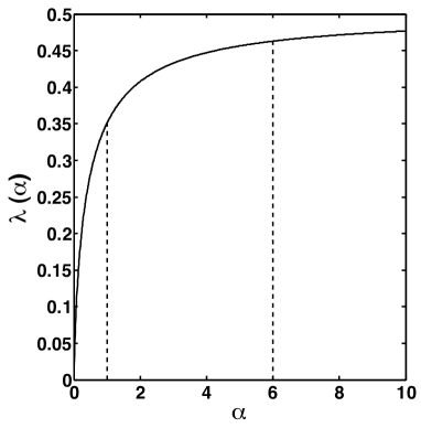
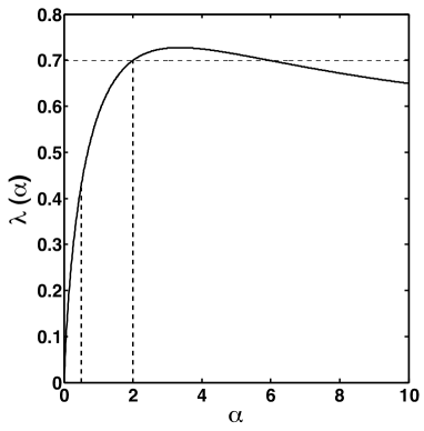
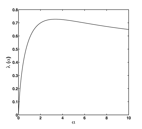
Thus in the class of constant controls, our optimization problem reduces to maximizing the Perron eigenvalue. The following Proposition gives an answer to this problem in the case of the running example (1.4) (see also Figure 1).
Refer to caption
Figure 1: Dominant eigenvalue of the matrix G+αF𝐺𝛼𝐹G+\alpha F as a function of the control parameter α𝛼\alpha. The function achieves a maximum for α=α(0,+)𝛼superscript𝛼0\alpha=\alpha^{*}\in(0,+\infty).
Proposition 2.1.

There exists a maximal eigenvalue λP(α)subscript𝜆𝑃superscript𝛼\lambda_{P}(\alpha^{*}) for some α(0,+)superscript𝛼0\alpha^{*}\in(0,+\infty) if and only if τ2>2τ1subscript𝜏22subscript𝜏1\tau_{2}>2\tau_{1}. Furthermore we have the following alternative:

  • either τ22τ1subscript𝜏22subscript𝜏1\tau_{2}\leq 2\tau_{1} and λP(α)subscript𝜆𝑃𝛼\lambda_{P}(\alpha) increases from 00 to τ1,subscript𝜏1\tau_{1},

  • or τ2>2τ1subscript𝜏22subscript𝜏1\tau_{2}>2\tau_{1} and λP(α)subscript𝜆𝑃𝛼\lambda_{P}(\alpha) first increases from 00 to λP(α)subscript𝜆𝑃superscript𝛼\lambda_{P}(\alpha^{*}) and then decreases to τ1.subscript𝜏1\tau_{1}.

Proof.

The characteristic polynomial of G+αF𝐺𝛼𝐹G+\alpha F is

P(X)=X3+(τ1+τ2+α(β2+β3))X2+(τ1τ2+ατ1(β3β2)+α2β2β3)Xατ1τ2β3α2τ1β2β3.𝑃𝑋superscript𝑋3subscript𝜏1subscript𝜏2𝛼subscript𝛽2subscript𝛽3superscript𝑋2subscript𝜏1subscript𝜏2𝛼subscript𝜏1subscript𝛽3subscript𝛽2superscript𝛼2subscript𝛽2subscript𝛽3𝑋𝛼subscript𝜏1subscript𝜏2subscript𝛽3superscript𝛼2subscript𝜏1subscript𝛽2subscript𝛽3P(X)=X^{3}+\left(\tau_{1}+\tau_{2}+\alpha(\beta_{2}+\beta_{3})\right)X^{2}+\left(\tau_{1}\tau_{2}+\alpha\tau_{1}(\beta_{3}-\beta_{2})+\alpha^{2}\beta_{2}\beta_{3}\right)X-\alpha\tau_{1}\tau_{2}\beta_{3}-\alpha^{2}\tau_{1}\beta_{2}\beta_{3}\,.

The Perron eigenvalue λP(α)subscript𝜆𝑃𝛼\lambda_{P}(\alpha) is the largest zero of this polynomial, so P(λP(α))=0𝑃subscript𝜆𝑃𝛼0P(\lambda_{P}(\alpha))=0 and, dividing by α2superscript𝛼2\alpha^{2} we get that that limα+λP(α)=τ1.subscript𝛼subscript𝜆𝑃𝛼subscript𝜏1\lim_{\alpha\to+\infty}\lambda_{P}(\alpha)=\tau_{1}. We easily check that P(λ)>0superscript𝑃𝜆0P^{\prime}(\lambda)>0 for λ>τ1𝜆subscript𝜏1\lambda>\tau_{1}, and we evaluate

P(τ1)=2τ12(τ1+τ2)+ατ1β3(2τ1τ2).𝑃subscript𝜏12superscriptsubscript𝜏12subscript𝜏1subscript𝜏2𝛼subscript𝜏1subscript𝛽32subscript𝜏1subscript𝜏2P(\tau_{1})=2\tau_{1}^{2}(\tau_{1}+\tau_{2})+\alpha\tau_{1}\beta_{3}(2\tau_{1}-\tau_{2})\,.

We have the following alternative: either τ2<2τ1subscript𝜏22subscript𝜏1\tau_{2}<2\tau_{1} and P(τ1)>0𝑃subscript𝜏10P(\tau_{1})>0 for all α>0𝛼0\alpha>0, or τ2>2τ1subscript𝜏22subscript𝜏1\tau_{2}>2\tau_{1} and P(τ1)<0𝑃subscript𝜏10P(\tau_{1})<0 for large α𝛼\alpha. In the former case, we have λP(α)<τ1subscript𝜆𝑃𝛼subscript𝜏1\lambda_{P}(\alpha)<\tau_{1} for all α>0𝛼0\alpha>0. In the latter case, we have λP(α)>τ1subscript𝜆𝑃𝛼subscript𝜏1\lambda_{P}(\alpha)>\tau_{1} for large α𝛼\alpha. On the other hand we have λP(0)=0subscript𝜆𝑃00\lambda_{P}(0)=0. Therefore, the condition τ2>2τ1subscript𝜏22subscript𝜏1\tau_{2}>2\tau_{1} is necessary and sufficient for λPsubscript𝜆𝑃\lambda_{P} to reach a global maximum.

Differentiating the relation P(λP(α))=0,𝑃subscript𝜆𝑃𝛼0P(\lambda_{P}(\alpha))=0, we get that any critical point α𝛼\alpha such that λP(α)=0superscriptsubscript𝜆𝑃𝛼0\lambda_{P}^{\prime}(\alpha)=0 satisfies

(β2+β3)λP(α)2+τ1(β3β2)λP(α)+2αβ2β3λP(α)=τ1τ2β2β3+2ατ1β2β3.subscript𝛽2subscript𝛽3subscript𝜆𝑃superscript𝛼2subscript𝜏1subscript𝛽3subscript𝛽2subscript𝜆𝑃𝛼2𝛼subscript𝛽2subscript𝛽3subscript𝜆𝑃𝛼subscript𝜏1subscript𝜏2subscript𝛽2subscript𝛽32𝛼subscript𝜏1subscript𝛽2subscript𝛽3(\beta_{2}+\beta_{3})\lambda_{P}(\alpha)^{2}+\tau_{1}(\beta_{3}-\beta_{2})\lambda_{P}(\alpha)+2\alpha\beta_{2}\beta_{3}\lambda_{P}(\alpha)=\tau_{1}\tau_{2}\beta_{2}\beta_{3}+2\alpha\tau_{1}\beta_{2}\beta_{3}\,. (2.2)

Differentiating twice the relation P(λP(α))=0,𝑃subscript𝜆𝑃𝛼0P(\lambda_{P}(\alpha))=0, we get that any such critical point α𝛼\alpha satisfies

λP′′(α)=2β2β3(τ1λP(α))3λP(α)2+2(τ1+τ2+α(β2+β3))λP(α)+τ1τ2+ατ1(β3β2)+α2β2β3.superscriptsubscript𝜆𝑃′′𝛼2subscript𝛽2subscript𝛽3subscript𝜏1subscript𝜆𝑃𝛼3subscript𝜆𝑃superscript𝛼22subscript𝜏1subscript𝜏2𝛼subscript𝛽2subscript𝛽3subscript𝜆𝑃𝛼subscript𝜏1subscript𝜏2𝛼subscript𝜏1subscript𝛽3subscript𝛽2superscript𝛼2subscript𝛽2subscript𝛽3\lambda_{P}^{\prime\prime}(\alpha)=\frac{2\beta_{2}\beta_{3}(\tau_{1}-\lambda_{P}(\alpha))}{3\lambda_{P}(\alpha)^{2}+2(\tau_{1}+\tau_{2}+\alpha(\beta_{2}+\beta_{3}))\lambda_{P}(\alpha)+\tau_{1}\tau_{2}+\alpha\tau_{1}(\beta_{3}-\beta_{2})+\alpha^{2}\beta_{2}\beta_{3}}.

We claim that the denominator is always positive, despite the possible negative terme ατ1(β3β2)𝛼subscript𝜏1subscript𝛽3subscript𝛽2\alpha\tau_{1}(\beta_{3}-\beta_{2}). In fact we can factorize by αβ2𝛼subscript𝛽2\alpha\beta_{2}: αβ2(λP(α)τ1)0𝛼subscript𝛽2subscript𝜆𝑃𝛼subscript𝜏10\alpha\beta_{2}\left(\lambda_{P}(\alpha)-\tau_{1}\right)\geq 0 if λP(α)τ1subscript𝜆𝑃𝛼subscript𝜏1\lambda_{P}(\alpha)\geq\tau_{1}. In the other case λP(α)τ1subscript𝜆𝑃𝛼subscript𝜏1\lambda_{P}(\alpha)\leq\tau_{1}, we use the relation (2.2) to get

2α(β2+β3)λP(α)+ατ1(β3β2)+α2β2β32𝛼subscript𝛽2subscript𝛽3subscript𝜆𝑃𝛼𝛼subscript𝜏1subscript𝛽3subscript𝛽2superscript𝛼2subscript𝛽2subscript𝛽3\displaystyle 2\alpha(\beta_{2}+\beta_{3})\lambda_{P}(\alpha)+\alpha\tau_{1}(\beta_{3}-\beta_{2})+\alpha^{2}\beta_{2}\beta_{3} αλP(α)(τ1τ2β2β3+2ατ1β2β3)α2β2β3absent𝛼subscript𝜆𝑃𝛼subscript𝜏1subscript𝜏2subscript𝛽2subscript𝛽32𝛼subscript𝜏1subscript𝛽2subscript𝛽3superscript𝛼2subscript𝛽2subscript𝛽3\displaystyle\geq\frac{\alpha}{\lambda_{P}(\alpha)}\left(\tau_{1}\tau_{2}\beta_{2}\beta_{3}+2\alpha\tau_{1}\beta_{2}\beta_{3}\right)-\alpha^{2}\beta_{2}\beta_{3}
α2λP(α)β2β3(2τ1λP(α))0.absentsuperscript𝛼2subscript𝜆𝑃𝛼subscript𝛽2subscript𝛽32subscript𝜏1subscript𝜆𝑃𝛼0\displaystyle\geq\frac{\alpha^{2}}{\lambda_{P}(\alpha)}\beta_{2}\beta_{3}\left(2\tau_{1}-\lambda_{P}(\alpha)\right)\geq 0\,.

In conclusion, λP′′(α)superscriptsubscript𝜆𝑃′′𝛼\lambda_{P}^{\prime\prime}(\alpha) has the same sign as τ1λP(α)subscript𝜏1subscript𝜆𝑃𝛼\tau_{1}-\lambda_{P}(\alpha) so λP(α)subscript𝜆𝑃𝛼\lambda_{P}(\alpha) can be a local minimum only if λP(α)τ1subscript𝜆𝑃𝛼subscript𝜏1\lambda_{P}(\alpha)\leq\tau_{1} and a local maximum only if λP(α)τ1.subscript𝜆𝑃𝛼subscript𝜏1\lambda_{P}(\alpha)\geq\tau_{1}. The alternative announced in the proposition follows. ∎

Next we consider a periodic control α(t)𝛼𝑡\alpha(t) with period θ>0𝜃0\theta>0. There exists a Floquet eigenvalue λF(α)subscript𝜆𝐹𝛼\lambda_{F}(\alpha) and periodic eigenvectors eα(t)subscript𝑒𝛼𝑡e_{\alpha}(t), ϕα(t)subscriptitalic-ϕ𝛼𝑡\phi_{\alpha}(t) such that

{ddteα(t)+λF(α)eα(t)=(G+α(t)F)eα(t),ddtϕα(t)+λF(α)ϕα(t)=ϕα(t)(G+α(t)F).cases𝑑𝑑𝑡subscript𝑒𝛼𝑡subscript𝜆𝐹𝛼subscript𝑒𝛼𝑡𝐺𝛼𝑡𝐹subscript𝑒𝛼𝑡𝑑𝑑𝑡subscriptitalic-ϕ𝛼𝑡subscript𝜆𝐹𝛼subscriptitalic-ϕ𝛼𝑡subscriptitalic-ϕ𝛼𝑡𝐺𝛼𝑡𝐹\left\{\begin{array}[]{l}\displaystyle\frac{d}{dt}e_{\alpha}(t)+\lambda_{F}(\alpha)e_{\alpha}(t)=(G+\alpha(t)F)e_{\alpha}(t)\,,\vskip 6.0pt plus 2.0pt minus 2.0pt\\ \displaystyle\frac{d}{dt}\phi_{\alpha}(t)+\lambda_{F}(\alpha)\phi_{\alpha}(t)=\phi_{\alpha}(t)(G+\alpha(t)F)\,.\end{array}\right.

These eigenfunctions are unique after normalization,

1θ0θm,eα(t)𝑑t=1,1θ0θϕα(t)eα(t)𝑑t=1.formulae-sequence1𝜃superscriptsubscript0𝜃𝑚subscript𝑒𝛼𝑡differential-d𝑡11𝜃superscriptsubscript0𝜃delimited-⟨⟩subscriptitalic-ϕ𝛼𝑡subscript𝑒𝛼𝑡differential-d𝑡1\dfrac{1}{\theta}\int_{0}^{\theta}\left\langle m,e_{\alpha}(t)\right\rangle\,dt=1\,,\quad\dfrac{1}{\theta}\int_{0}^{\theta}\left\langle\phi_{\alpha}(t)e_{\alpha}(t)\right\rangle\,dt=1\,.

Again we obtain the following expansion for the payoff,

rα(T,x)=λF(α)+1T(logϕα(0),x+logm,eα(T))+o(1T).subscript𝑟𝛼𝑇𝑥subscript𝜆𝐹𝛼1𝑇subscriptitalic-ϕ𝛼0𝑥𝑚subscript𝑒𝛼𝑇𝑜1𝑇r_{\alpha}(T,x)=\lambda_{F}(\alpha)+\frac{1}{T}\Big{(}\log\langle\phi_{\alpha}(0),x\rangle+\log\langle m,e_{\alpha}(T)\rangle\Big{)}+o\left(\frac{1}{T}\right)\,.

A natural problem is to find periodic controls α(t)𝛼𝑡\alpha(t) such that the Floquet eigenvalue is better than the optimal Perron eigenvalue λP(α)subscript𝜆𝑃superscript𝛼\lambda_{P}(\alpha^{*}). The following Proposition gives a partial answer to this question. We consider small periodic perturbations of the best constant control: α(t)=α+ϵγ(t)𝛼𝑡superscript𝛼italic-ϵ𝛾𝑡\alpha(t)=\alpha^{*}+\epsilon\gamma(t), where γ𝛾\gamma is a given θ𝜃\theta-periodic function. For the sake of clarity we introduce the following notation for the time average over a period,

fθ=1θ0θf(t)𝑑t.subscriptdelimited-⟨⟩𝑓𝜃1𝜃superscriptsubscript0𝜃𝑓𝑡differential-d𝑡\langle f\rangle_{\theta}=\frac{1}{\theta}\int_{0}^{\theta}f(t)\,dt\,.

We assume that the matrix G+αF𝐺superscript𝛼𝐹G+\alpha^{*}F is diagonalizable (in \mathbb{R}). This is the case for the running example (see Appendix A). We denote by (e1,e2,e3)superscriptsubscript𝑒1superscriptsubscript𝑒2superscriptsubscript𝑒3(e_{1}^{*},e_{2}^{*},e_{3}^{*}) and (ϕ1,ϕ2,ϕ3)superscriptsubscriptitalic-ϕ1superscriptsubscriptitalic-ϕ2superscriptsubscriptitalic-ϕ3(\phi_{1}^{*},\phi_{2}^{*},\phi_{3}^{*}) the bases of right- and left- eigenvectors associated to the eigenvalues λ1,λ2,λ3superscriptsubscript𝜆1superscriptsubscript𝜆2superscriptsubscript𝜆3\lambda_{1}^{*},\lambda_{2}^{*},\lambda_{3}^{*} for the the best constant control αsuperscript𝛼\alpha^{*}. Notice that according to previous notations we have e1=eαsuperscriptsubscript𝑒1subscript𝑒superscript𝛼e_{1}^{*}=e_{\alpha^{*}} and λ1=λP(α)superscriptsubscript𝜆1subscript𝜆𝑃superscript𝛼\lambda_{1}^{*}=\lambda_{P}(\alpha^{*}).

Proposition 2.2.

The directional derivative of the dominant eigenvalue vanishes at ϵ=0italic-ϵ0\epsilon=0:

dλF(α+ϵγ)dϵ|ϵ=0=0.evaluated-at𝑑subscript𝜆𝐹superscript𝛼italic-ϵ𝛾𝑑italic-ϵitalic-ϵ00\left.\dfrac{d\lambda_{F}(\alpha^{*}+\epsilon\gamma)}{d\epsilon}\right|_{\epsilon=0}=0\,. (2.3)

Hence, αsuperscript𝛼\alpha^{*} is also a critical point in the class of periodic controls. The second directional derivative of the dominant eigenvalue writes at ϵ=0italic-ϵ0\epsilon=0:

d2λF(α+ϵγ)dϵ2|ϵ=0=2i=23γi2θ(ϕ1Fei)(ϕiFe1)λ1λi,evaluated-atsuperscript𝑑2subscript𝜆𝐹superscript𝛼italic-ϵ𝛾𝑑superscriptitalic-ϵ2italic-ϵ02superscriptsubscript𝑖23subscriptdelimited-⟨⟩superscriptsubscript𝛾𝑖2𝜃superscriptsubscriptitalic-ϕ1𝐹superscriptsubscript𝑒𝑖superscriptsubscriptitalic-ϕ𝑖𝐹superscriptsubscript𝑒1superscriptsubscript𝜆1superscriptsubscript𝜆𝑖\left.\dfrac{d^{2}\lambda_{F}(\alpha^{*}+\epsilon\gamma)}{d\epsilon^{2}}\right|_{\epsilon=0}=2\sum_{i=2}^{3}\langle\gamma_{i}^{2}\rangle_{\theta}\frac{(\phi_{1}^{*}Fe_{i}^{*})(\phi_{i}^{*}Fe_{1}^{*})}{\lambda_{1}^{*}-\lambda_{i}^{*}}\,, (2.4)

where γi(t)subscript𝛾𝑖𝑡\gamma_{i}(t) is the unique θ𝜃\theta-periodic function which is solution to the relaxation ODE

γi˙(t)λ1λi+γi(t)=γ(t).˙subscript𝛾𝑖𝑡superscriptsubscript𝜆1superscriptsubscript𝜆𝑖subscript𝛾𝑖𝑡𝛾𝑡\dfrac{\dot{\gamma_{i}}(t)}{\lambda_{1}^{*}-\lambda_{i}^{*}}+\gamma_{i}(t)=\gamma(t)\,.

The idea of computing directional derivatives has been used in a similar context in [24] for optimizing the Perron eigenvalue in a continuous model for cell division.

Taking γ1𝛾1\gamma\equiv 1 in Equation (2.4), we get the second derivative of the Perron eigenvalue at αsuperscript𝛼\alpha^{*},

d2λPdα2(α)=2i=23(ϕ1Fei)(ϕiFe1)λ1λi,superscript𝑑2subscript𝜆𝑃𝑑superscript𝛼2superscript𝛼2superscriptsubscript𝑖23superscriptsubscriptitalic-ϕ1𝐹superscriptsubscript𝑒𝑖superscriptsubscriptitalic-ϕ𝑖𝐹superscriptsubscript𝑒1superscriptsubscript𝜆1superscriptsubscript𝜆𝑖\dfrac{d^{2}\lambda_{P}}{d\alpha^{2}}(\alpha^{*})=2\sum_{i=2}^{3}\dfrac{(\phi_{1}^{*}Fe_{i}^{*})(\phi_{i}^{*}Fe_{1}^{*})}{\lambda_{1}^{*}-\lambda_{i}^{*}}\,, (2.5)

which is nonpositive since αsuperscript𝛼\alpha^{*} is a maximum point. However we cannot conclude directly in the general case that the quantity (2.4) is nonpositive since we do not know the relative signs of the coefficients (ϕ1Fei)(ϕiFe1)superscriptsubscriptitalic-ϕ1𝐹superscriptsubscript𝑒𝑖superscriptsubscriptitalic-ϕ𝑖𝐹superscriptsubscript𝑒1(\phi_{1}^{*}Fe_{i}^{*})(\phi_{i}^{*}Fe_{1}^{*}) in (2.5).

We study in [14] a variant of (1.1), where the control is not affine. We prove that there exist directions γ𝛾\gamma for which αsuperscript𝛼\alpha^{*} is a minimum point. Alternatively speaking, periodic controls can beat the best constant control. For this, we perturb the constant control with high-frequency modes, and we compute the limit of d2λFdϵ2superscript𝑑2subscript𝜆𝐹𝑑superscriptitalic-ϵ2\frac{d^{2}\lambda_{F}}{d\epsilon^{2}} when the frequency tends to infinity. Unfortunately, this procedure gives no additional information in the case of an affine control.

Proof of Proposition 2.2.

First we derive a formula for the first derivative of the Perron eigenvalue: By definition we have

(G+αF)eα=λP(α)eα.𝐺𝛼𝐹subscript𝑒𝛼subscript𝜆𝑃𝛼subscript𝑒𝛼(G+\alpha F)e_{\alpha}=\lambda_{P}(\alpha)e_{\alpha}\,.

Deriving with respect to α𝛼\alpha we get

dλPdα(α)eα+λP(α)deαdα=Feα+(G+αF)deαdα.𝑑subscript𝜆𝑃𝑑𝛼𝛼subscript𝑒𝛼subscript𝜆𝑃𝛼𝑑subscript𝑒𝛼𝑑𝛼𝐹subscript𝑒𝛼𝐺𝛼𝐹𝑑subscript𝑒𝛼𝑑𝛼\frac{d\lambda_{P}}{d\alpha}(\alpha)e_{\alpha}+\lambda_{P}(\alpha)\frac{de_{\alpha}}{d\alpha}=Fe_{\alpha}+(G+\alpha F)\frac{de_{\alpha}}{d\alpha}\,.

Testing against the left- eigenvector ϕαsubscriptitalic-ϕ𝛼\phi_{\alpha} we obtain

dλPdα(α)=ϕαFeα.𝑑subscript𝜆𝑃𝑑𝛼𝛼subscriptitalic-ϕ𝛼𝐹subscript𝑒𝛼\frac{d\lambda_{P}}{d\alpha}(\alpha)=\phi_{\alpha}Fe_{\alpha}\,.

Second, we write the Floquet eigenvalue problem corresponding to the periodic control α=α+ϵγ𝛼superscript𝛼italic-ϵ𝛾\alpha=\alpha^{*}+\epsilon\gamma:

teα(t)+λF(α+ϵγ)eα(t)=(G+(α+ϵγ(t))F)eα(t).𝑡subscript𝑒𝛼𝑡subscript𝜆𝐹superscript𝛼italic-ϵ𝛾subscript𝑒𝛼𝑡𝐺superscript𝛼italic-ϵ𝛾𝑡𝐹subscript𝑒𝛼𝑡\frac{\partial}{\partial t}e_{\alpha}(t)+\lambda_{F}(\alpha^{*}+\epsilon\gamma)e_{\alpha}(t)=(G+(\alpha^{*}+\epsilon\gamma(t))F)e_{\alpha}(t)\,.

Deriving this ODE with respect to ϵitalic-ϵ\epsilon, we get

teαϵ(t)+dλF(α+ϵγ)dϵeα(t)+λF(α+ϵγ)eαϵ(t)=γ(t)Feα(t)+(G+(α+ϵγ(t))F)eαϵ(t).𝑡subscript𝑒𝛼italic-ϵ𝑡𝑑subscript𝜆𝐹superscript𝛼italic-ϵ𝛾𝑑italic-ϵsubscript𝑒𝛼𝑡subscript𝜆𝐹superscript𝛼italic-ϵ𝛾subscript𝑒𝛼italic-ϵ𝑡𝛾𝑡𝐹subscript𝑒𝛼𝑡𝐺superscript𝛼italic-ϵ𝛾𝑡𝐹subscript𝑒𝛼italic-ϵ𝑡\frac{\partial}{\partial t}\dfrac{\partial e_{\alpha}}{\partial\epsilon}(t)+\dfrac{d\lambda_{F}(\alpha^{*}+\epsilon\gamma)}{d\epsilon}e_{\alpha}(t)+\lambda_{F}(\alpha^{*}+\epsilon\gamma)\dfrac{\partial e_{\alpha}}{\partial\epsilon}(t)=\gamma(t)Fe_{\alpha}(t)+(G+(\alpha^{*}+\epsilon\gamma(t))F)\dfrac{\partial e_{\alpha}}{\partial\epsilon}(t)\,. (2.6)

Testing this equation against ϕ1superscriptsubscriptitalic-ϕ1\phi_{1}^{*} and evaluating at ϵ=0italic-ϵ0\epsilon=0, we obtain

t(ϕ1eαϵ|ϵ=0(t))+dλF(α+ϵγ)dϵ|ϵ=0=γ(t)ϕ1Fe1.𝑡evaluated-atsuperscriptsubscriptitalic-ϕ1subscript𝑒𝛼italic-ϵitalic-ϵ0𝑡evaluated-at𝑑subscript𝜆𝐹superscript𝛼italic-ϵ𝛾𝑑italic-ϵitalic-ϵ0𝛾𝑡superscriptsubscriptitalic-ϕ1𝐹superscriptsubscript𝑒1\frac{\partial}{\partial t}\left(\phi_{1}^{*}\left.\dfrac{\partial e_{\alpha}}{\partial\epsilon}\right|_{\epsilon=0}(t)\right)+\left.\dfrac{d\lambda_{F}(\alpha^{*}+\epsilon\gamma)}{d\epsilon}\right|_{\epsilon=0}=\gamma(t)\phi_{1}^{*}Fe_{1}^{*}\,.

After integration over one period, we get

dλF(α+ϵγ)dϵ|ϵ=0=(1θ0θγ(t)𝑑t)ϕ1Fe1=γθdλPdα(α)=0,evaluated-at𝑑subscript𝜆𝐹superscript𝛼italic-ϵ𝛾𝑑italic-ϵitalic-ϵ01𝜃superscriptsubscript0𝜃𝛾𝑡differential-d𝑡superscriptsubscriptitalic-ϕ1𝐹superscriptsubscript𝑒1subscriptdelimited-⟨⟩𝛾𝜃𝑑subscript𝜆𝑃𝑑𝛼superscript𝛼0\left.\dfrac{d\lambda_{F}(\alpha^{*}+\epsilon\gamma)}{d\epsilon}\right|_{\epsilon=0}=\left(\frac{1}{\theta}\int_{0}^{\theta}\gamma(t)\,dt\right)\phi_{1}^{*}Fe_{1}^{*}=\left\langle\gamma\right\rangle_{\theta}\dfrac{d\lambda_{P}}{d\alpha}(\alpha^{*})=0\,,

which is the first order condition (2.3).

Next, we test (2.6) against another left- eigenvector ϕisuperscriptsubscriptitalic-ϕ𝑖\phi_{i}^{*} and we evaluate at ϵ=0italic-ϵ0\epsilon=0. We obtain the following equation satisfied by γi(t)=(λ1λi)ϕieαϵ(t)(ϕiFe1)1subscript𝛾𝑖𝑡superscriptsubscript𝜆1superscriptsubscript𝜆𝑖superscriptsubscriptitalic-ϕ𝑖subscript𝑒𝛼italic-ϵ𝑡superscriptsuperscriptsubscriptitalic-ϕ𝑖𝐹superscriptsubscript𝑒11\gamma_{i}(t)=(\lambda_{1}^{*}-\lambda_{i}^{*})\phi_{i}^{*}\dfrac{\partial e_{\alpha}}{\partial\epsilon}(t)(\phi_{i}^{*}Fe_{1}^{*})^{-1}:

1λ1λitγi(t)+γi(t)=γ(t).1superscriptsubscript𝜆1superscriptsubscript𝜆𝑖𝑡subscript𝛾𝑖𝑡subscript𝛾𝑖𝑡𝛾𝑡\frac{1}{\lambda_{1}^{*}-\lambda_{i}^{*}}\frac{\partial}{\partial t}{\gamma_{i}}(t)+\gamma_{i}(t)=\gamma(t)\,. (2.7)

We differentiate (2.6) with respect to ϵitalic-ϵ\epsilon. This yields

t2eαϵ2(t)+d2λF(α+ϵγ)dϵ2eα(t)+2dλF(α+ϵγ)dϵeαϵ(t)+λF(α+ϵγ)2eαϵ2(t)=2γ(t)Feαϵ(t)+(G+(α+ϵγ(t))F)2eαϵ2(t).𝑡superscript2subscript𝑒𝛼superscriptitalic-ϵ2𝑡superscript𝑑2subscript𝜆𝐹superscript𝛼italic-ϵ𝛾𝑑superscriptitalic-ϵ2subscript𝑒𝛼𝑡2𝑑subscript𝜆𝐹superscript𝛼italic-ϵ𝛾𝑑italic-ϵsubscript𝑒𝛼italic-ϵ𝑡subscript𝜆𝐹superscript𝛼italic-ϵ𝛾superscript2subscript𝑒𝛼superscriptitalic-ϵ2𝑡2𝛾𝑡𝐹subscript𝑒𝛼italic-ϵ𝑡𝐺superscript𝛼italic-ϵ𝛾𝑡𝐹superscript2subscript𝑒𝛼superscriptitalic-ϵ2𝑡\frac{\partial}{\partial t}\dfrac{\partial^{2}e_{\alpha}}{\partial\epsilon^{2}}(t)+\dfrac{d^{2}\lambda_{F}(\alpha^{*}+\epsilon\gamma)}{d\epsilon^{2}}e_{\alpha}(t)+2\dfrac{d\lambda_{F}(\alpha^{*}+\epsilon\gamma)}{d\epsilon}\dfrac{\partial e_{\alpha}}{\partial\epsilon}(t)+\lambda_{F}(\alpha^{*}+\epsilon\gamma)\dfrac{\partial^{2}e_{\alpha}}{\partial\epsilon^{2}}(t)\\ =2\gamma(t)F\dfrac{\partial e_{\alpha}}{\partial\epsilon}(t)+(G+(\alpha^{*}+\epsilon\gamma(t))F)\dfrac{\partial^{2}e_{\alpha}}{\partial\epsilon^{2}}(t)\,.

Testing this equation against ϕ1superscriptsubscriptitalic-ϕ1\phi_{1}^{*} and evaluating at ϵ=0italic-ϵ0\epsilon=0, we find

t(ϕ12eαϵ2|ϵ=0(t))+d2λF(α+ϵγ)dϵ2|ϵ=0=2γ(t)ϕ1Feαϵ|ϵ=0(t).𝑡evaluated-atsuperscriptsubscriptitalic-ϕ1superscript2subscript𝑒𝛼superscriptitalic-ϵ2italic-ϵ0𝑡evaluated-atsuperscript𝑑2subscript𝜆𝐹superscript𝛼italic-ϵ𝛾𝑑superscriptitalic-ϵ2italic-ϵ0evaluated-at2𝛾𝑡superscriptsubscriptitalic-ϕ1𝐹subscript𝑒𝛼italic-ϵitalic-ϵ0𝑡\frac{\partial}{\partial t}\left(\phi_{1}^{*}\left.\dfrac{\partial^{2}e_{\alpha}}{\partial\epsilon^{2}}\right|_{\epsilon=0}(t)\right)+\left.\dfrac{d^{2}\lambda_{F}(\alpha^{*}+\epsilon\gamma)}{d\epsilon^{2}}\right|_{\epsilon=0}=2\gamma(t)\phi_{1}^{*}F\left.\dfrac{\partial e_{\alpha}}{\partial\epsilon}\right|_{\epsilon=0}(t)\,. (2.8)

We decompose the unknown eαϵ(t)subscript𝑒𝛼italic-ϵ𝑡\frac{\partial e_{\alpha}}{\partial\epsilon}(t) along the basis (e1,e2,e3)superscriptsubscript𝑒1superscriptsubscript𝑒2superscriptsubscript𝑒3(e_{1}^{*},e_{2}^{*},e_{3}^{*})

eαϵ(t)=i=13γi(t)(ϕiFe1)λ1λiei.subscript𝑒𝛼italic-ϵ𝑡superscriptsubscript𝑖13subscript𝛾𝑖𝑡superscriptsubscriptitalic-ϕ𝑖𝐹superscriptsubscript𝑒1superscriptsubscript𝜆1superscriptsubscript𝜆𝑖superscriptsubscript𝑒𝑖\frac{\partial e_{\alpha}}{\partial\epsilon}(t)=\sum_{i=1}^{3}\gamma_{i}(t)\frac{(\phi_{i}^{*}Fe_{1}^{*})}{\lambda_{1}^{*}-\lambda_{i}^{*}}e_{i}^{*}\,.

In particular, we have

ϕ1Feαϵ(t)=i=23γi(t)(ϕiFe1)λ1λi(ϕ1Fei),superscriptsubscriptitalic-ϕ1𝐹subscript𝑒𝛼italic-ϵ𝑡superscriptsubscript𝑖23subscript𝛾𝑖𝑡superscriptsubscriptitalic-ϕ𝑖𝐹superscriptsubscript𝑒1superscriptsubscript𝜆1superscriptsubscript𝜆𝑖superscriptsubscriptitalic-ϕ1𝐹superscriptsubscript𝑒𝑖\phi_{1}^{*}F\dfrac{\partial e_{\alpha}}{\partial\epsilon}(t)=\sum_{i=2}^{3}\gamma_{i}(t)\frac{(\phi_{i}^{*}Fe_{1}^{*})}{\lambda_{1}^{*}-\lambda_{i}^{*}}(\phi_{1}^{*}Fe_{i}^{*})\,,

since ϕ1Fe1=0superscriptsubscriptitalic-ϕ1𝐹superscriptsubscript𝑒10\phi_{1}^{*}Fe_{1}^{*}=0 by optimality. To conclude, we integrate (2.8) over one period,

d2λF(α+ϵγ)dϵ2|ϵ=0=2i=23γγiθ(ϕiFe1)(ϕ1Fei)λ1λi.evaluated-atsuperscript𝑑2subscript𝜆𝐹superscript𝛼italic-ϵ𝛾𝑑superscriptitalic-ϵ2italic-ϵ02superscriptsubscript𝑖23subscriptdelimited-⟨⟩𝛾subscript𝛾𝑖𝜃superscriptsubscriptitalic-ϕ𝑖𝐹superscriptsubscript𝑒1superscriptsubscriptitalic-ϕ1𝐹superscriptsubscript𝑒𝑖superscriptsubscript𝜆1superscriptsubscript𝜆𝑖\left.\dfrac{d^{2}\lambda_{F}(\alpha^{*}+\epsilon\gamma)}{d\epsilon^{2}}\right|_{\epsilon=0}=2\sum_{i=2}^{3}\langle\gamma\gamma_{i}\rangle_{\theta}\dfrac{(\phi_{i}^{*}Fe_{1}^{*})(\phi_{1}^{*}Fe_{i}^{*})}{\lambda_{1}^{*}-\lambda_{i}^{*}}\,.

We conclude thanks to the following identity derived from (2.7): γi2θ=γγiθsubscriptdelimited-⟨⟩superscriptsubscript𝛾𝑖2𝜃subscriptdelimited-⟨⟩𝛾subscript𝛾𝑖𝜃\left\langle\gamma_{i}^{2}\right\rangle_{\theta}=\langle\gamma\gamma_{i}\rangle_{\theta}. ∎

3 Optimal control and the ergodic problem

Let a,A𝑎𝐴a,A be some given bounds on the control parameter α𝛼\alpha, with a<α<A𝑎superscript𝛼𝐴a<\alpha^{*}<A. Let T>0𝑇0T>0 be a (large) time. The optimal control problem associated to (1.1) reads as follows

V(T,x)=supα{m,xα(T):x˙α(t)=(G+α(t)F)xα(t),xα(0)=x},𝑉𝑇𝑥subscriptsupremum𝛼conditional-set𝑚subscript𝑥𝛼𝑇formulae-sequencesubscript˙𝑥𝛼𝑡𝐺𝛼𝑡𝐹subscript𝑥𝛼𝑡subscript𝑥𝛼0𝑥V(T,x)=\sup_{\alpha}\left\{\left\langle m,x_{\alpha}(T)\right\rangle\;:\;\dot{x}_{\alpha}(t)=(G+\alpha(t)F)x_{\alpha}(t)\;,\;x_{\alpha}(0)=x\right\}\,,

where the supremum is taken over all measurable control functions α:(0,T)[a,A]:𝛼0𝑇𝑎𝐴\alpha:(0,T)\to[a,A]. The principle of dynamic programming enables to solve this optimal control problem by introducing the value function v(s,x)=sup{m,xα(T):x˙α(t)=(G+α(t)F)xα(t),xα(s)=x}𝑣𝑠𝑥supremumconditional-set𝑚subscript𝑥𝛼𝑇formulae-sequencesubscript˙𝑥𝛼𝑡𝐺𝛼𝑡𝐹subscript𝑥𝛼𝑡subscript𝑥𝛼𝑠𝑥v(s,x)=\sup\left\{\left\langle m,x_{\alpha}(T)\right\rangle\;:\;\dot{x}_{\alpha}(t)=(G+\alpha(t)F)x_{\alpha}(t)\;,\;x_{\alpha}(s)=x\right\}. We have v(T,x)=m,x𝑣𝑇𝑥𝑚𝑥v(T,x)=\left\langle m,x\right\rangle, v(0,x)=V(T,x)𝑣0𝑥𝑉𝑇𝑥v(0,x)=V(T,x), and v𝑣v satisfies the following Hamilton-Jacobi-Bellman equation in the viscosity sense,

sv(s,x)+H~(x,Dxv(s,x))=0,𝑠𝑣𝑠𝑥~𝐻𝑥subscript𝐷𝑥𝑣𝑠𝑥0\frac{\partial}{\partial s}v(s,x)+\widetilde{H}(x,D_{x}v(s,x))=0\,,

where the Hamiltonian is given by H~(x,p)=maxα[a,A]{(G+αF)x,p}~𝐻𝑥𝑝subscript𝛼𝑎𝐴𝐺𝛼𝐹𝑥𝑝\widetilde{H}(x,p)=\max_{\alpha\in[a,A]}\left\{\left\langle(G+\alpha F)x,p\right\rangle\right\}. This equation is backward in time: the initial data is prescribed at the final time s=T𝑠𝑇s=T.

Intuitively we expect an exponential growth of the reward m,xα(T)𝑚subscript𝑥𝛼𝑇\left\langle m,x_{\alpha}(T)\right\rangle as T+𝑇T\to+\infty. This motivates the following reduction to a compact space/linear growth.

3.1 Reduction to a compact space/linear growth

We perform a logarithmic change of variable: w(s,x)=logv(s,x)logm,x𝑤𝑠𝑥𝑣𝑠𝑥𝑚𝑥w(s,x)=\log v(s,x)-\log\left\langle m,x\right\rangle. The reward function satisfies:

ddtlogm,xα(t)=m,x˙α(t)m,xα(t)=m,(G+α(t)F)yα(t)=m,Gyα(t),𝑑𝑑𝑡𝑚subscript𝑥𝛼𝑡𝑚subscript˙𝑥𝛼𝑡𝑚subscript𝑥𝛼𝑡𝑚𝐺𝛼𝑡𝐹subscript𝑦𝛼𝑡𝑚𝐺subscript𝑦𝛼𝑡\dfrac{d}{dt}\log\left\langle m,x_{\alpha}(t)\right\rangle=\dfrac{\left\langle m,\dot{x}_{\alpha}(t)\right\rangle}{\left\langle m,x_{\alpha}(t)\right\rangle}=\left\langle m,(G+\alpha(t)F)y_{\alpha}(t)\right\rangle=\left\langle m,Gy_{\alpha}(t)\right\rangle\,,

where y=xm,x𝑦𝑥𝑚𝑥y=\frac{x}{\left\langle m,x\right\rangle} denotes the projection on the simplex 𝒮={y0:m,y=1}𝒮conditional-set𝑦0𝑚𝑦1\mathcal{S}=\{y\geq 0\;:\;\left\langle m,y\right\rangle=1\}. We can write a close equation for the projected trajectory yα(t)subscript𝑦𝛼𝑡y_{\alpha}(t) due to the linearity of the system:

y˙α(t)subscript˙𝑦𝛼𝑡\displaystyle\dot{y}_{\alpha}(t) =x˙α(t)m,xα(t)xα(t)m,xα(t)m,x˙α(t)m,xα(t)absentsubscript˙𝑥𝛼𝑡𝑚subscript𝑥𝛼𝑡subscript𝑥𝛼𝑡𝑚subscript𝑥𝛼𝑡𝑚subscript˙𝑥𝛼𝑡𝑚subscript𝑥𝛼𝑡\displaystyle=\frac{\dot{x}_{\alpha}(t)}{\left\langle m,x_{\alpha}(t)\right\rangle}-\frac{x_{\alpha}(t)}{\left\langle m,x_{\alpha}(t)\right\rangle}\frac{\left\langle m,\dot{x}_{\alpha}(t)\right\rangle}{\left\langle m,x_{\alpha}(t)\right\rangle}
=(G+α(t)F)yα(t)m,(G+α(t)F)yα(t)yα(t)absent𝐺𝛼𝑡𝐹subscript𝑦𝛼𝑡𝑚𝐺𝛼𝑡𝐹subscript𝑦𝛼𝑡subscript𝑦𝛼𝑡\displaystyle=(G+\alpha(t)F)y_{\alpha}(t)-\left\langle m,(G+\alpha(t)F)y_{\alpha}(t)\right\rangle y_{\alpha}(t)
=(G+α(t)F)yα(t)m,Gyα(t)yα(t),absent𝐺𝛼𝑡𝐹subscript𝑦𝛼𝑡𝑚𝐺subscript𝑦𝛼𝑡subscript𝑦𝛼𝑡\displaystyle=(G+\alpha(t)F)y_{\alpha}(t)-\left\langle m,Gy_{\alpha}(t)\right\rangle y_{\alpha}(t)\,,

(recall mTF=0superscript𝑚𝑇𝐹0m^{T}F=0). We introduce the following notation for the vector field on the simplex:

b(y,α)=(G+αF)ym,Gyy.𝑏𝑦𝛼𝐺𝛼𝐹𝑦𝑚𝐺𝑦𝑦b(y,\alpha)=(G+\alpha F)y-\left\langle m,Gy\right\rangle y\,.

It is worth mentioning that the only stationary point of the vector field b(y,α)𝑏𝑦𝛼b(y,\alpha) on the simplex 𝒮𝒮\mathcal{S} is the dominant eigenvector eαsubscript𝑒𝛼e_{\alpha}: b(eα,α)=0𝑏subscript𝑒𝛼𝛼0b(e_{\alpha},\alpha)=0. Furthermore, for any y𝒮𝑦𝒮y\in\mathcal{S} the trajectory starting from y𝑦y with constant control α(t)α𝛼𝑡𝛼\alpha(t)\equiv\alpha converges to eαsubscript𝑒𝛼e_{\alpha} as t+𝑡t\to+\infty, and leaves the simplex 𝒮𝒮\mathcal{S} as t𝑡t\to-\infty. Moreover the vector field b(y,α)𝑏𝑦𝛼b(y,\alpha) can be easily computed on each eigenvector y=eβ𝑦subscript𝑒𝛽y=e_{\beta} due to the affine structure of the problem:

b(eβ,α)𝑏subscript𝑒𝛽𝛼\displaystyle b(e_{\beta},\alpha) =(G+αF)eβm,Geβeβabsent𝐺𝛼𝐹subscript𝑒𝛽𝑚𝐺subscript𝑒𝛽subscript𝑒𝛽\displaystyle=(G+\alpha F)e_{\beta}-\left\langle m,Ge_{\beta}\right\rangle e_{\beta}
=(αβ)Feβ+b(eβ,β)absent𝛼𝛽𝐹subscript𝑒𝛽𝑏subscript𝑒𝛽𝛽\displaystyle=(\alpha-\beta)Fe_{\beta}+b(e_{\beta},\beta)
=(αβ)Feβ.absent𝛼𝛽𝐹subscript𝑒𝛽\displaystyle=(\alpha-\beta)Fe_{\beta}\,.

The logarithmic value function w𝑤w satisfies the following optimization problem for x𝒮𝑥𝒮x\in\mathcal{S}:

w(s,x)=supα{logm,xα(T)logm,x}=supα{sTm,Gyα(t)𝑑t:y˙α(t)=b(yα(t),α(t)),yα(s)=x}𝑤𝑠𝑥subscriptsupremum𝛼𝑚subscript𝑥𝛼𝑇𝑚𝑥subscriptsupremum𝛼conditional-setsuperscriptsubscript𝑠𝑇𝑚𝐺subscript𝑦𝛼𝑡differential-d𝑡formulae-sequencesubscript˙𝑦𝛼𝑡𝑏subscript𝑦𝛼𝑡𝛼𝑡subscript𝑦𝛼𝑠𝑥w(s,x)=\sup_{\alpha}\left\{\log\left\langle m,x_{\alpha}(T)\right\rangle-\log\left\langle m,x\right\rangle\right\}=\sup_{\alpha}\left\{\int_{s}^{T}\left\langle m,Gy_{\alpha}(t)\right\rangle\,dt\;:\;\dot{y}_{\alpha}(t)=b(y_{\alpha}(t),\alpha(t))\;,\;y_{\alpha}(s)=x\right\}

Finally for notational convenience, we perform the time reversal t=Ts𝑡𝑇𝑠t=T-s, and introduce u(t,y)=w(Tt,y)𝑢𝑡𝑦𝑤𝑇𝑡𝑦u(t,y)=w(T-t,y) for y𝒮𝑦𝒮y\in\mathcal{S}. The optimal problem is now reduced to a compact space (the simplex 𝒮𝒮\mathcal{S}), with a running reward:

u(t,y)=supα{0tL(yα(s))𝑑s:y˙α(s)=b(yα(s),α(s)),yα(0)=y}.𝑢𝑡𝑦subscriptsupremum𝛼conditional-setsuperscriptsubscript0𝑡𝐿subscript𝑦𝛼𝑠differential-d𝑠formulae-sequencesubscript˙𝑦𝛼𝑠𝑏subscript𝑦𝛼𝑠𝛼𝑠subscript𝑦𝛼0𝑦u(t,y)=\sup_{\alpha}\left\{\int_{0}^{t}L(y_{\alpha}(s))\,ds\;:\;\dot{y}_{\alpha}(s)=b(y_{\alpha}(s),\alpha(s))\;,\;y_{\alpha}(0)=y\right\}\,.

where the reward function is linear: L(y)=m,Gy𝐿𝑦𝑚𝐺𝑦L(y)=\left\langle m,Gy\right\rangle. The function u𝑢-u is a viscosity solution of the following Hamilton-Jacobi equation:

{t(u(t,y))+H(y,Dyu(t,y))=0,u(0,y)=0,cases𝑡𝑢𝑡𝑦𝐻𝑦subscript𝐷𝑦𝑢𝑡𝑦0𝑢0𝑦0\left\{\begin{array}[]{l}\dfrac{\partial}{\partial t}(-u(t,y))+H(y,D_{y}u(t,y))=0\,,\vskip 6.0pt plus 2.0pt minus 2.0pt\\ u(0,y)=0\,,\end{array}\right. (3.1)

where the Hamiltonian is given by

H(y,p)=maxα[a,A]{b(y,α),p+m,Gy}.𝐻𝑦𝑝subscript𝛼𝑎𝐴𝑏𝑦𝛼𝑝𝑚𝐺𝑦H(y,p)=\max_{\alpha\in[a,A]}\left\{\left\langle b(y,\alpha),p\right\rangle+\left\langle m,Gy\right\rangle\right\}\,. (3.2)
Remark 3.1.

An important observation is that this hamiltonian does not satisfy the classical coercivity assumption H(,p)+𝐻𝑝H(\cdot,p)\to+\infty as |p|+𝑝|p|\to+\infty. Indeed for all y𝒮𝑦𝒮y\in\mathcal{S} there exists a cone C(y)𝐶𝑦C(y) such that H(y,p)𝐻𝑦𝑝H(y,p)\to-\infty if pC(y)𝑝𝐶𝑦p\in C(y) and |p|+𝑝|p|\to+\infty. In addition we have C(y)=𝐶𝑦C(y)=\emptyset if and only if y=eβ𝑦subscript𝑒𝛽y=e_{\beta} for some β0𝛽0\beta\geq 0. In the latter case we have

H(eβ,p)=maxα[a,A]{(αβ)Feβ,p}+L(eβ)=(Aβ)Feβ,p++(βa)Feβ,p+λP(β).𝐻subscript𝑒𝛽𝑝subscript𝛼𝑎𝐴𝛼𝛽𝐹subscript𝑒𝛽𝑝𝐿subscript𝑒𝛽𝐴𝛽subscript𝐹subscript𝑒𝛽𝑝𝛽𝑎subscript𝐹subscript𝑒𝛽𝑝subscript𝜆𝑃𝛽H(e_{\beta},p)=\max_{\alpha\in[a,A]}\{\left\langle(\alpha-\beta)Fe_{\beta},p\right\rangle\}+L(e_{\beta})=(A-\beta)\left\langle Fe_{\beta},p\right\rangle_{+}+(\beta-a)\left\langle Fe_{\beta},p\right\rangle_{-}+\lambda_{P}(\beta)\,.

It is not coercive either.

Due to the lack of coercivity the ergodic problem is difficult to handle with. We follow the procedure described in [2, 3] to exhibit an ergodic set in the simplex. This set has to fulfill two important features: controllability, and attractivity. We construct below such an ergodic set, and we prove the two required properties.

3.2 Notations and statement of the result

Following [3] we introduce the auxiliary problem with infinite horizon:

uϵ(y)=supα{0+eϵtL(yα(t))𝑑t:y˙α(t)=b(yα(t),α(t)),yα(0)=y}.subscript𝑢italic-ϵ𝑦subscriptsupremum𝛼conditional-setsuperscriptsubscript0superscript𝑒italic-ϵ𝑡𝐿subscript𝑦𝛼𝑡differential-d𝑡formulae-sequencesubscript˙𝑦𝛼𝑡𝑏subscript𝑦𝛼𝑡𝛼𝑡subscript𝑦𝛼0𝑦u_{\epsilon}(y)=\sup_{\alpha}\left\{\int_{0}^{+\infty}e^{-\epsilon t}L(y_{\alpha}(t))\,dt\;:\;\dot{y}_{\alpha}(t)=b(y_{\alpha}(t),\alpha(t))\;,\;y_{\alpha}(0)=y\right\}\,. (3.3)

The limit of the quantity ϵuϵ(y)italic-ϵsubscript𝑢italic-ϵ𝑦\epsilon u_{\epsilon}(y) as ϵ0italic-ϵ0\epsilon\to 0 measures the convergence of the reward L(y(t))𝐿𝑦𝑡L(y(t)) as t+𝑡t\to+\infty in average (convergence à la Césaro). The function u𝑢-u is a viscosity solution of the following stationary Hamilton-Jacobi equation:

ϵuϵ(y)+H(y,Dyuϵ(y))=0.italic-ϵsubscript𝑢italic-ϵ𝑦𝐻𝑦subscript𝐷𝑦subscript𝑢italic-ϵ𝑦0-\epsilon u_{\epsilon}(y)+H(y,D_{y}u_{\epsilon}(y))=0\,. (3.4)

The next Theorem claims that the function ϵuϵ(y)italic-ϵsubscript𝑢italic-ϵ𝑦\epsilon u_{\epsilon}(y) converges to a constant. We interpret this constant as the (generalized) eigenvalue associated to the optimal control problem.

We introduce some notations necessary for the statement of the two technical hypotheses (H4-5):

  • 𝒮𝒮\mathcal{S}: the simplex {y0:m,y=1}conditional-set𝑦0𝑚𝑦1\{y\geq 0\;:\;\left\langle m,y\right\rangle=1\},

  • ΘΘ\Theta: the (direct) orthogonal rotation with angle π/2𝜋2\pi/2 on the tangent space T𝒮𝑇𝒮T\mathcal{S},

  • Φ0={eα|α+}𝒮subscriptΦ0conditional-setsubscript𝑒𝛼𝛼subscript𝒮\Phi_{0}=\{e_{\alpha}\;|\;\alpha\in\mathbb{R}_{+}\}\subset\mathcal{S}: the set of Perron eigenvectors,

(H4)

We assume a first technical condition:

deαdα,ΘFeαhas a constant sign for α0.𝑑subscript𝑒𝛼𝑑𝛼Θ𝐹subscript𝑒𝛼has a constant sign for α0.\left\langle\frac{de_{\alpha}}{d\alpha},\Theta Fe_{\alpha}\right\rangle\quad\text{has a constant sign for $\alpha\geq 0$.} (3.5)

This hypothesis enables to determine the direction of the vector field b(y,α)𝑏𝑦𝛼b(y,\alpha) accross Φ0subscriptΦ0\Phi_{0} at y=eβ𝑦subscript𝑒𝛽y=e_{\beta}:

Θdeαdα|α=β,b(eβ,α)=(αβ)deαdα|α=β,ΘFeβ.evaluated-atΘ𝑑subscript𝑒𝛼𝑑𝛼𝛼𝛽𝑏subscript𝑒𝛽𝛼𝛼𝛽evaluated-at𝑑subscript𝑒𝛼𝑑𝛼𝛼𝛽Θ𝐹subscript𝑒𝛽\left\langle\Theta\left.\frac{de_{\alpha}}{d\alpha}\right|_{\alpha=\beta},b(e_{\beta},\alpha)\right\rangle=-(\alpha-\beta)\left\langle\left.\frac{de_{\alpha}}{d\alpha}\right|_{\alpha=\beta},\Theta Fe_{\beta}\right\rangle\,. (3.6)

Due to Hypothesis (H4), only the sign of αβ𝛼𝛽\alpha-\beta determines the sign of the above quantity.

We assume without loss of generality that the quantity (3.5) is negative for all α0𝛼0\alpha\geq 0. This has been checked numerically in the case of the running example (1.4) (see Appendix B).

(H5)

We assume a second technical condition: there exists δ0>0subscript𝛿00\delta_{0}>0 such that for any constant control β(Aδ0,A+δ0)𝛽𝐴subscript𝛿0𝐴subscript𝛿0\beta\in(A-\delta_{0},A+\delta_{0}), the trajectory starting from e0subscript𝑒0e_{0} with constant control β𝛽\beta, which connects e0subscript𝑒0e_{0} and eβsubscript𝑒𝛽e_{\beta}, does not cross the curve Φ0subscriptΦ0\Phi_{0} for t>0𝑡0t>0. Similarly, for any constant control β(aδ0,a+δ0)𝛽𝑎subscript𝛿0𝑎subscript𝛿0\beta\in(a-\delta_{0},a+\delta_{0}), the trajectory starting from esubscript𝑒e_{\infty} with constant control β𝛽\beta, which connects esubscript𝑒e_{\infty} and eβsubscript𝑒𝛽e_{\beta}, does not cross the curve Φ0subscriptΦ0\Phi_{0}.

A proper construction of some remarkable sets in the proof of the following Theorem relies on these two technical assumptions, e.g. 𝒵0,𝒯±subscript𝒵0subscript𝒯plus-or-minus\mathcal{Z}_{0},\mathcal{T}_{\pm} (Figures 2 and 5).

Theorem 3.2 (Ergodicity).

Assume that hypotheses (H1-2-3-4-5) are satisfied. There exists a constant λHJsubscript𝜆𝐻𝐽\lambda_{HJ} such that the following uniform convergence holds true:

limϵ0ϵuϵ(y)=λHJ,uniformly for y𝒮.subscriptitalic-ϵ0italic-ϵsubscript𝑢italic-ϵ𝑦subscript𝜆𝐻𝐽uniformly for y𝒮\lim_{\epsilon\to 0}\epsilon u_{\epsilon}(y)=\lambda_{HJ}\,,\quad\text{uniformly for $y\in\mathcal{S}$}\,.

The constant λHJsubscript𝜆𝐻𝐽\lambda_{HJ} is interpreted as the eigenvalue associated to the Hamiltonian H(y,p)𝐻𝑦𝑝H(y,p). We are not able to prove the existence of an eigenvector here. Indeed we lack an equicontinuity estimate on the family (uϵ)ϵsubscriptsubscript𝑢italic-ϵitalic-ϵ(u_{\epsilon})_{\epsilon}. We only obtain equicontinuity of the family (ϵuϵ)ϵsubscriptitalic-ϵsubscript𝑢italic-ϵitalic-ϵ(\epsilon u_{\epsilon})_{\epsilon}. However we postulate such an eigenvector does exist, based on numerical evidence (see Section 4).

Corollary 3.3.

Assume that hypotheses (H1-2-3-4-5) are satisfied. Then the solution of the Hamilton-Jacobi-Bellman equation satisfies the following ergodic property:

limT+u(T,y)T=λHJ,uniformly for y𝒮.subscript𝑇𝑢𝑇𝑦𝑇subscript𝜆𝐻𝐽uniformly for y𝒮\lim_{T\to+\infty}\dfrac{u(T,y)}{T}=\lambda_{HJ}\,,\quad\text{uniformly for $y\in\mathcal{S}$}\,.

Back to the original problem, Corollary 3.3 translates into (1.2), where convergence is uniform on compact subsets of (+)3{0}superscriptsubscript30\left(\mathbb{R}_{+}\right)^{3}\setminus\{0\}.

3.3 Proof of Theorem 3.2

We mainly follow [3] with some refinements specific to our context. We proceed in several steps, with illustrative figures to facilitate the argumentation.

The program is the following: we identify the so-called ergodic set 𝒵0𝒮subscript𝒵0𝒮\mathcal{Z}_{0}\subset\mathcal{S} [2, 3], and we show some of its interesting properties. We begin with the controllability problem. Controllability enables to prove convergence to the constant λHJsubscript𝜆𝐻𝐽\lambda_{HJ} when y𝑦y belongs to the ergodic set 𝒵0subscript𝒵0\mathcal{Z}_{0}. Next we demonstrate the attractiveness of the ergodic set 𝒵0subscript𝒵0\mathcal{Z}_{0}. This enables to extend the convergence to every y𝒮𝑦𝒮y\in\mathcal{S}.

There is a technical subtlety concerning the time required for controllability/attractiveness. This time could degenerate as we get close to the boundary of the ergodic set. We circumvent this issue by proving that close-to-optimal trajectories do not stay in the vicinity of the boundary for long time.

Step 1- Identification of some remarkable sets: the set of eigenvectors, and the ergodic set.

The first remarkable subset of the simplex 𝒮𝒮\mathcal{S} is the set of eigenvectors Φ0={eα|α+}subscriptΦ0conditional-setsubscript𝑒𝛼𝛼subscript\Phi_{0}=\{e_{\alpha}\;|\;\alpha\in\mathbb{R}_{+}\}. It is alternatively defined as the zero level set of the cubic function

φ(y)=b(y,α),ΘFy=Gym,Gyy,ΘFy.𝜑𝑦𝑏𝑦𝛼Θ𝐹𝑦𝐺𝑦𝑚𝐺𝑦𝑦Θ𝐹𝑦\varphi(y)=\left\langle b(y,\alpha),\Theta Fy\right\rangle=\left\langle Gy-\left\langle m,Gy\right\rangle y,\Theta Fy\right\rangle\,.

Hence we have,

Φ0={eα|α+}={y𝒮:φ(y)=0}.subscriptΦ0conditional-setsubscript𝑒𝛼𝛼subscriptconditional-set𝑦𝒮𝜑𝑦0\Phi_{0}=\{e_{\alpha}\;|\;\alpha\in\mathbb{R}_{+}\}=\{y\in\mathcal{S}\;:\;\varphi(y)=0\}\,.

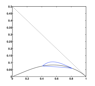
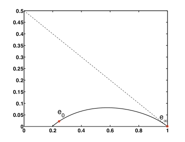
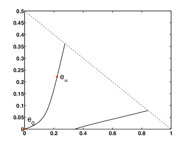
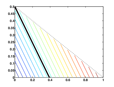
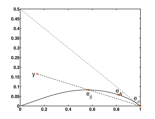
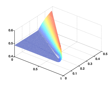
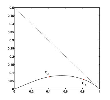
Indeed, y𝒮𝑦𝒮y\in\mathcal{S} is an eigenvector if and only if there exists α𝛼\alpha such that (G+αF)ym,Gyy=0𝐺𝛼𝐹𝑦𝑚𝐺𝑦𝑦0(G+\alpha F)y-\left\langle m,Gy\right\rangle y=0, i.e. Gym,Gyyspan(Fy)𝐺𝑦𝑚𝐺𝑦𝑦span𝐹𝑦Gy-\left\langle m,Gy\right\rangle y\in\mathrm{span}\,(Fy), or equivalently Gym,GyyΘFyperpendicular-to𝐺𝑦𝑚𝐺𝑦𝑦Θ𝐹𝑦Gy-\left\langle m,Gy\right\rangle y\perp\Theta Fy. From Hypothesis (H3) we deduce that Φ0subscriptΦ0\Phi_{0} is a curve connecting two boundary points of the simplex 𝒮𝒮\mathcal{S}. In Figure 2 we have plotted the set of eigenvectors in the case of the running example.

The set of eigenvector splits the simplex 𝒮𝒮\mathcal{S} into two subsets, denoted by Φ+subscriptΦ\Phi_{+} and ΦsubscriptΦ\Phi_{-}, respectively:

Φ+={y𝒮:φ(y)0},Φ={y𝒮:φ(y)0}.\Phi_{+}=\{y\in\mathcal{S}\;:\;\varphi(y)\geq 0\}\quad,\quad\Phi_{-}=\{y\in\mathcal{S}\;:\;\varphi(y)\leq 0\}\,.

Notice that the sign of φ𝜑\varphi depends on the orientation of the rotation ΘΘ\Theta. Obviously the following discussion does not depend on this convention.
Refer to caption

(a) Refer to caption(b)

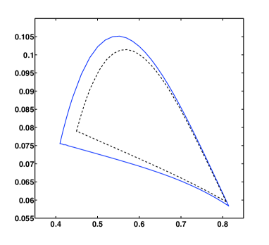
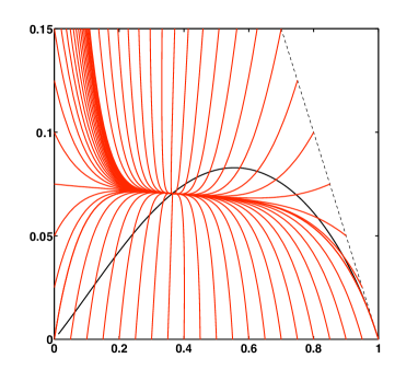
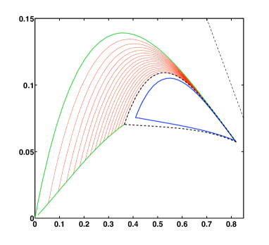
Figure 2: The set of eigenvectors Φ0subscriptΦ0\Phi_{0} (a) and the boundary of the ergodic set 𝒵0subscript𝒵0\mathcal{Z}_{0} (b). The dashed line represent the boundary of the simplex.

We seek the ergodic set which is stable, attractant and controllable. The natural candidate is defined through its boundary as follows. The boundary consists of two curves which are joining on the set Φ0subscriptΦ0\Phi_{0}.

Definition 3.4.

The ergodic set 𝒵0subscript𝒵0\mathcal{Z}_{0} is the compact set enclosed by the two following curves:

γaA{γ˙(s)=b(γ(s),a)γ(0)=eA,γAa{γ˙(s)=b(γ(s),A)γ(0)=ea.superscriptsubscript𝛾𝑎𝐴casesotherwise˙𝛾𝑠𝑏𝛾𝑠𝑎otherwise𝛾0subscript𝑒𝐴superscriptsubscript𝛾𝐴𝑎casesotherwise˙𝛾𝑠𝑏𝛾𝑠𝐴otherwise𝛾0subscript𝑒𝑎\gamma_{a}^{A}\begin{cases}&\dot{\gamma}(s)=b(\gamma(s),a)\\ &\gamma(0)=e_{A}\end{cases}\,,\quad\gamma_{A}^{a}\begin{cases}&\dot{\gamma}(s)=b(\gamma(s),A)\\ &\gamma(0)=e_{a}\end{cases}\,. (3.7)

The set 𝒵0subscript𝒵0\mathcal{Z}_{0} is well defined. In fact we have lims+γaA(s)=easubscript𝑠superscriptsubscript𝛾𝑎𝐴𝑠subscript𝑒𝑎\lim_{s\to+\infty}\gamma_{a}^{A}(s)=e_{a} and lims+γAa(s)=eAsubscript𝑠superscriptsubscript𝛾𝐴𝑎𝑠subscript𝑒𝐴\lim_{s\to+\infty}\gamma_{A}^{a}(s)=e_{A}.

In Figure 2 we have plotted an example of the ergodic set 𝒵0subscript𝒵0\mathcal{Z}_{0} for the running example. We list in the following Proposition some useful properties of the set 𝒵0subscript𝒵0\mathcal{Z}_{0} which are derived from the very definition.

Lemma 3.5.
  1. (i)

    The curves γaA,γAasubscriptsuperscript𝛾𝐴𝑎subscriptsuperscript𝛾𝑎𝐴\gamma^{A}_{a},\gamma^{a}_{A} lie on the opposite sides of Φ0subscriptΦ0\Phi_{0}. We assume without loss of generality that the curve γaAsubscriptsuperscript𝛾𝐴𝑎\gamma^{A}_{a} belongs to the subset Φ+subscriptΦ\Phi_{+}, whereas the curve γAasubscriptsuperscript𝛾𝑎𝐴\gamma^{a}_{A} belongs to the subset ΦsubscriptΦ\Phi_{-}.

  2. (ii)

    The set 𝒵0subscript𝒵0\mathcal{Z}_{0} is stable: the vector fields {b(y,α),α[a,A]}𝑏𝑦𝛼𝛼𝑎𝐴\{b(y,\alpha)\;,\;\alpha\in[a,A]\} are all pointing inwards on the boundary of 𝒵0subscript𝒵0\mathcal{Z}_{0}.

Proof.

(i) We denote by γA0superscriptsubscript𝛾𝐴0\gamma_{A}^{0} the trajectory connecting e0subscript𝑒0e_{0} to eAsubscript𝑒𝐴e_{A} with constant control A𝐴A. Similarly we denote by γasuperscriptsubscript𝛾𝑎\gamma_{a}^{\infty} the trajectory connecting esubscript𝑒e_{\infty} to easubscript𝑒𝑎e_{a} with constant control a𝑎a. From Hypothesis (H4) these two trajectories initially start on the two opposite sides of the line of eigenvectors Φ0subscriptΦ0\Phi_{0}. Notice that γasuperscriptsubscript𝛾𝑎\gamma_{a}^{\infty} may start tangentially to Φ0subscriptΦ0\Phi_{0} (it is actually the case for the running example). However a continuity argument for γaβsuperscriptsubscript𝛾𝑎𝛽\gamma_{a}^{\beta} with β+𝛽\beta\to+\infty yields the statement. Hypothesis (H5) guarantees that they do not cross Φ0subscriptΦ0\Phi_{0}, so that they stay on opposite sides of Φ0subscriptΦ0\Phi_{0} forever. We assume without loss of generality that γA0superscriptsubscript𝛾𝐴0\gamma_{A}^{0} lies in ΦsubscriptΦ\Phi_{-} and γasuperscriptsubscript𝛾𝑎\gamma_{a}^{\infty} lies in Φ+subscriptΦ\Phi_{+}.

Second from the bounds on the control aα(t)A𝑎𝛼𝑡𝐴a\leq\alpha(t)\leq A, together with Hypothesis (H4) (3.6), the trajectory γAasuperscriptsubscript𝛾𝐴𝑎\gamma_{A}^{a} starts on the same side as γA0superscriptsubscript𝛾𝐴0\gamma_{A}^{0} (i.e. ΦsubscriptΦ\Phi_{-} with the above convention). Moreover it cannot cross the line of eigenvectors Φ0subscriptΦ0\Phi_{0} at eβsubscript𝑒𝛽e_{\beta} for β(0,A)𝛽0𝐴\beta\in(0,A). From the uniqueness theorem for ODE, it cannot cross the trajectory γA0superscriptsubscript𝛾𝐴0\gamma_{A}^{0} either. As a conclusion, the trajectory γAasuperscriptsubscript𝛾𝐴𝑎\gamma_{A}^{a} is sandwiched between the portion of Φ0subscriptΦ0\Phi_{0} between e0subscript𝑒0e_{0} and eAsubscript𝑒𝐴e_{A}, and γA0superscriptsubscript𝛾𝐴0\gamma_{A}^{0}. Therefore it belongs to ΦsubscriptΦ\Phi_{-}.

The same holds true for γaAΦ+superscriptsubscript𝛾𝑎𝐴subscriptΦ\gamma_{a}^{A}\subset\Phi_{+}.

(ii) We denote by n(z)𝑛𝑧n(z) the unit vector normal and exterior to the boundary of 𝒵0subscript𝒵0\mathcal{Z}_{0}. We have more precisely:

na(z)=Θb(z,a)|Θb(z,a)|on γaA,nA(z)=Θb(z,A)|Θb(z,A)|on γAa.n_{a}(z)=\dfrac{\Theta b(z,a)}{|\Theta b(z,a)|}\quad\mbox{on $\gamma^{A}_{a}$}\quad,\quad n_{A}(z)=\dfrac{\Theta b(z,A)}{|\Theta b(z,A)|}\quad\mbox{on $\gamma^{a}_{A}$}\,.

We have on the one side γaAsubscriptsuperscript𝛾𝐴𝑎\gamma^{A}_{a}: α[a,A]b(z,α),na(z)b(z,a),na(z)=0for-all𝛼𝑎𝐴𝑏𝑧𝛼subscript𝑛𝑎𝑧𝑏𝑧𝑎subscript𝑛𝑎𝑧0\forall\alpha\in[a,A]\;\left\langle b(z,\alpha),n_{a}(z)\right\rangle\leq\left\langle b(z,a),n_{a}(z)\right\rangle=0. Indeed we have

b(z,α)b(z,a),na(z)𝑏𝑧𝛼𝑏𝑧𝑎subscript𝑛𝑎𝑧\displaystyle\left\langle b(z,\alpha)-b(z,a),n_{a}(z)\right\rangle =(αa)Fz,na(z)absent𝛼𝑎𝐹𝑧subscript𝑛𝑎𝑧\displaystyle=(\alpha-a)\left\langle Fz,n_{a}(z)\right\rangle
=(αa)ΘFz,Θna(z)absent𝛼𝑎Θ𝐹𝑧Θsubscript𝑛𝑎𝑧\displaystyle=(\alpha-a)\left\langle\Theta Fz,\Theta n_{a}(z)\right\rangle
=(αa)ΘFz,b(z,a)|b(z,a)|absent𝛼𝑎Θ𝐹𝑧𝑏𝑧𝑎𝑏𝑧𝑎\displaystyle=(\alpha-a)\left\langle\Theta Fz,-\dfrac{b(z,a)}{|b(z,a)|}\right\rangle
=(aα)|b(z,a)|ΘFz,Gzm,Gzz0.absent𝑎𝛼𝑏𝑧𝑎Θ𝐹𝑧𝐺𝑧𝑚𝐺𝑧𝑧0\displaystyle=\dfrac{(a-\alpha)}{|b(z,a)|}\left\langle\Theta Fz,Gz-\left\langle m,Gz\right\rangle z\right\rangle\leq 0\,.

We have on the other side γAasubscriptsuperscript𝛾𝑎𝐴\gamma^{a}_{A}:

b(z,α)b(z,A),nA(z)=(αA)Fz,nA(z)=(Aα)|b(z,A)|φ(z)0.𝑏𝑧𝛼𝑏𝑧𝐴subscript𝑛𝐴𝑧𝛼𝐴𝐹𝑧subscript𝑛𝐴𝑧𝐴𝛼𝑏𝑧𝐴𝜑𝑧0\left\langle b(z,\alpha)-b(z,A),n_{A}(z)\right\rangle=(\alpha-A)\left\langle Fz,n_{A}(z)\right\rangle=\dfrac{(A-\alpha)}{|b(z,A)|}\varphi(z)\leq 0\,.

Step 2- Exact controllability inside the ergodic set.

The purpose of this step is to prove the following Lemma 3.6, which asserts exact controllability in the ergodic set, except a narrow band. First we introduce some notations:

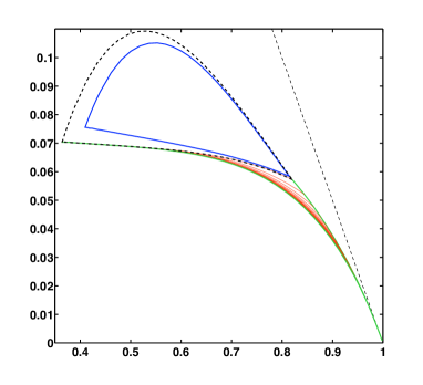
  • 𝒵δsubscript𝒵𝛿\mathcal{Z}_{-\delta} denotes the ergodic set, from which we have substracted a narrow band close to the boundary γaAγAasubscriptsuperscript𝛾𝐴𝑎subscriptsuperscript𝛾𝑎𝐴\gamma^{A}_{a}\cup\gamma^{a}_{A} (Figure 3). It is defined similarly as 𝒵0subscript𝒵0\mathcal{Z}_{0} by the delimitation of the two following curves,

    γa+δAδ{γ˙(s)=b(γ(s),a+δ)γ(0)=eAδ,γAδa+δ{γ˙(s)=b(γ(s),Aδ)γ(0)=ea+δ.subscriptsuperscript𝛾𝐴𝛿𝑎𝛿casesotherwise˙𝛾𝑠𝑏𝛾𝑠𝑎𝛿otherwise𝛾0subscript𝑒𝐴𝛿subscriptsuperscript𝛾𝑎𝛿𝐴𝛿casesotherwise˙𝛾𝑠𝑏𝛾𝑠𝐴𝛿otherwise𝛾0subscript𝑒𝑎𝛿\gamma^{A-\delta}_{a+\delta}\begin{cases}&\dot{\gamma}(s)=b(\gamma(s),a+\delta)\\ &\gamma(0)=e_{A-\delta}\end{cases}\,,\quad\gamma^{a+\delta}_{A-\delta}\begin{cases}&\dot{\gamma}(s)=b(\gamma(s),A-\delta)\\ &\gamma(0)=e_{a+\delta}\end{cases}\,.
  • 𝒵+2δsubscript𝒵2𝛿\mathcal{Z}_{+2\delta} denotes the ergodic set, to which we have added a narrow band close to the boundary γaAγAasubscriptsuperscript𝛾𝐴𝑎subscriptsuperscript𝛾𝑎𝐴\gamma^{A}_{a}\cup\gamma^{a}_{A} (Figure 5). It is defined similarly as 𝒵0subscript𝒵0\mathcal{Z}_{0} by the delimitation of the two following curves,

    γa2δA+2δ{γ˙(s)=b(γ(s),a2δ)γ(0)=eA+2δ,γA+2δa2δ{γ˙(s)=b(γ(s),A+2δ)γ(0)=ea2δ.subscriptsuperscript𝛾𝐴2𝛿𝑎2𝛿casesotherwise˙𝛾𝑠𝑏𝛾𝑠𝑎2𝛿otherwise𝛾0subscript𝑒𝐴2𝛿subscriptsuperscript𝛾𝑎2𝛿𝐴2𝛿casesotherwise˙𝛾𝑠𝑏𝛾𝑠𝐴2𝛿otherwise𝛾0subscript𝑒𝑎2𝛿\gamma^{A+2\delta}_{a-2\delta}\begin{cases}&\dot{\gamma}(s)=b(\gamma(s),a-2\delta)\\ &\gamma(0)=e_{A+2\delta}\end{cases}\,,\quad\gamma^{a-2\delta}_{A+2\delta}\begin{cases}&\dot{\gamma}(s)=b(\gamma(s),A+2\delta)\\ &\gamma(0)=e_{a-2\delta}\end{cases}\,.
Lemma 3.6.

The system y˙(t)=b(y(t),α)˙𝑦𝑡𝑏𝑦𝑡𝛼\dot{y}(t)=b(y(t),\alpha) is exactly controllable in the subset 𝒵δsubscript𝒵𝛿\mathcal{Z}_{-\delta}. For any z𝑧z, zsuperscript𝑧z^{\prime} in 𝒵δsubscript𝒵𝛿\mathcal{Z}_{-\delta} there exists a time T=T(z,z)𝑇𝑇𝑧superscript𝑧T=T(z,z^{\prime}) and α(t):[0,T][a,A]:𝛼𝑡0𝑇𝑎𝐴\alpha(t):[0,T]\to[a,A] such that y(0)=z𝑦0𝑧y(0)=z and y(T)=z𝑦𝑇superscript𝑧y(T)=z^{\prime}. Moreover it is possible to construct the control α(t)𝛼𝑡\alpha(t) following a bang-bang procedure: α(t):[0,T]{a,A}:𝛼𝑡0𝑇𝑎𝐴\alpha(t):[0,T]\to\{a,A\}. Last, the minimal time T𝑇T needed to connect z𝑧z and zsuperscript𝑧z^{\prime} is uniformly bounded for z,z𝒵δ𝑧superscript𝑧subscript𝒵𝛿z,z^{\prime}\in\mathcal{Z}_{-\delta}.

Refer to caption

(a) Refer to caption(b)

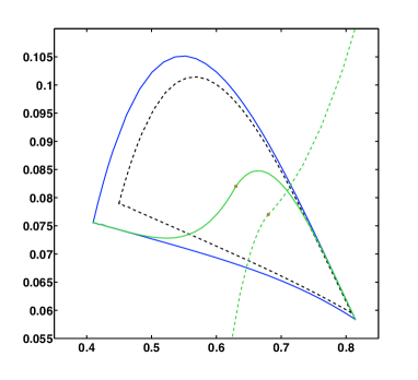
Figure 3: (a) The ergodic set 𝒵0subscript𝒵0\mathcal{Z}_{0} and the set 𝒵δsubscript𝒵𝛿\mathcal{Z}_{-\delta} (dashed line). (b) Illustration for the proof of the exact controllability in the set 𝒵δsubscript𝒵𝛿\mathcal{Z}_{-\delta}: the two curves Y𝑌Y (plain line) and Ysuperscript𝑌Y^{\prime} (dashed line) necessarily intersect in 𝒵0subscript𝒵0\mathcal{Z}_{0}.
Proof.

We aim at sending z𝑧z onto zsuperscript𝑧z^{\prime}. We define the trajectories yasubscript𝑦𝑎y_{a} and yAsubscript𝑦𝐴y_{A} starting from y𝑦y as follows,

ya{y˙a(t)=b(ya(t),a)ya(0)=z,yA{y˙A(t)=b(yA(t),A)yA(0)=z.subscript𝑦𝑎casesotherwisesubscript˙𝑦𝑎𝑡𝑏subscript𝑦𝑎𝑡𝑎otherwisesubscript𝑦𝑎0𝑧subscript𝑦𝐴casesotherwisesubscript˙𝑦𝐴𝑡𝑏subscript𝑦𝐴𝑡𝐴otherwisesubscript𝑦𝐴0𝑧y_{a}\begin{cases}&\dot{y}_{a}(t)=b(y_{a}(t),a)\\ &y_{a}(0)=z\end{cases}\,,\quad y_{A}\begin{cases}&\dot{y}_{A}(t)=b(y_{A}(t),A)\\ &y_{A}(0)=z\end{cases}\,.

When we concatenate the two trajectories Y=yayA𝑌subscript𝑦𝑎subscript𝑦𝐴Y=y_{a}\cup y_{A}, we obtain a curve which connects a𝑎a and A𝐴A. Reversing time, we define two other trajectories starting from zsuperscript𝑧z^{\prime},

ya{y˙a(t)=b(ya(t),a)ya(0)=z,yA{y˙A(t)=b(yA(t),A)yA(0)=z.subscriptsuperscript𝑦𝑎casesotherwisesubscriptsuperscript˙𝑦𝑎𝑡𝑏subscriptsuperscript𝑦𝑎𝑡𝑎otherwisesubscriptsuperscript𝑦𝑎0superscript𝑧subscriptsuperscript𝑦𝐴casesotherwisesubscriptsuperscript˙𝑦𝐴𝑡𝑏subscriptsuperscript𝑦𝐴𝑡𝐴otherwisesubscriptsuperscript𝑦𝐴0superscript𝑧y^{\prime}_{a}\begin{cases}&\dot{y}^{\prime}_{a}(t)=-b(y^{\prime}_{a}(t),a)\\ &y^{\prime}_{a}(0)=z^{\prime}\end{cases}\,,\quad y^{\prime}_{A}\begin{cases}&\dot{y}^{\prime}_{A}(t)=-b(y^{\prime}_{A}(t),A)\\ &y^{\prime}_{A}(0)=z^{\prime}\end{cases}\,.

Concatening the two trajectories we obtain a curve Y=yayAsuperscript𝑌superscriptsubscript𝑦𝑎superscriptsubscript𝑦𝐴Y^{\prime}=y_{a}^{\prime}\cup y_{A}^{\prime} which leaves the simplex 𝒮𝒮\mathcal{S}. Moreover it leaves the ergodic set 𝒵0subscript𝒵0\mathcal{Z}_{0} by the two opposite sides γAasubscriptsuperscript𝛾𝑎𝐴\gamma^{a}_{A} and γaAsubscriptsuperscript𝛾𝐴𝑎\gamma^{A}_{a}. Indeed yasuperscriptsubscript𝑦𝑎y_{a}^{\prime} cannot intersect γaAsubscriptsuperscript𝛾𝐴𝑎\gamma^{A}_{a}, and yAsuperscriptsubscript𝑦𝐴y_{A}^{\prime} cannot intersect γAasubscriptsuperscript𝛾𝑎𝐴\gamma^{a}_{A} by the uniqueness theorem for ODE. It necessarily intersects the curve Y𝑌Y since the latter connects a𝑎a and A𝐴A.

Let z′′YYsuperscript𝑧′′𝑌superscript𝑌z^{\prime\prime}\in Y\cap Y^{\prime}. We assume without loss of generality that z′′=ya(T)superscript𝑧′′subscript𝑦𝑎𝑇z^{\prime\prime}=y_{a}(T) and also z′′=yA(T)superscript𝑧′′subscriptsuperscript𝑦𝐴superscript𝑇z^{\prime\prime}=y^{\prime}_{A}(T^{\prime}). Observe that we do not necessarily have z′′𝒵δsuperscript𝑧′′subscript𝒵𝛿z^{\prime\prime}\in\mathcal{Z}_{-\delta}. However we do have z′′𝒵0superscript𝑧′′subscript𝒵0z^{\prime\prime}\in\mathcal{Z}_{0} since the set 𝒵0subscript𝒵0\mathcal{Z}_{0} is stable. Finally we construct the control α𝛼\alpha as follows: (i) from time t=0𝑡0t=0 to t=T𝑡𝑇t=T we set α(t)a𝛼𝑡𝑎\alpha(t)\equiv a, (ii) from t=T𝑡𝑇t=T to t=T+T𝑡𝑇superscript𝑇t=T+T^{\prime} we set α(t)A𝛼𝑡𝐴\alpha(t)\equiv A. This control sends z𝑧z onto zsuperscript𝑧z^{\prime} within time T+T𝑇superscript𝑇T+T^{\prime}.

The time Tsuperscript𝑇T^{\prime} is clearly uniformly bounded. To prove that the time T𝑇T is also uniformly bounded for z,z𝒵δ𝑧superscript𝑧subscript𝒵𝛿z,z^{\prime}\in\mathcal{Z}_{-\delta}, it is sufficient to avoid small neighbourhoods of the stationary points easubscript𝑒𝑎e_{a} and eAsubscript𝑒𝐴e_{A}. The image of 𝒵δsubscript𝒵𝛿\mathcal{Z}_{-\delta} by the backward trajectories yasuperscriptsubscript𝑦𝑎y_{a}^{\prime} and yAsuperscriptsubscript𝑦𝐴y_{A}^{\prime} inside 𝒵0subscript𝒵0\mathcal{Z}_{0} is a compact set which does not contain easubscript𝑒𝑎e_{a} nor eAsubscript𝑒𝐴e_{A}. Therefore the time T𝑇T is uniformly bounded. ∎

Step 3- Proof of the convergence towards λHJsubscript𝜆𝐻𝐽\lambda_{HJ} in the set 𝒵δsubscript𝒵𝛿\mathcal{Z}_{-\delta}.

We are now ready to prove an important lemma, which is a weaker version of Theorem 3.2.

Lemma 3.7.

Under the same assumptions as above, there exists a constant λHJsubscript𝜆𝐻𝐽\lambda_{HJ} such that the following uniform convergence holds true:

limϵ0ϵuϵ(z)=λHJ,uniformly for z𝒵δ.subscriptitalic-ϵ0italic-ϵsubscript𝑢italic-ϵ𝑧subscript𝜆𝐻𝐽uniformly for z𝒵δ\lim_{\epsilon\to 0}\epsilon u_{\epsilon}(z)=\lambda_{HJ}\,,\quad\text{uniformly for $z\in\mathcal{Z}_{-\delta}$}\,.
Proof.

First we observe that the function ϵuϵ(y)italic-ϵsubscript𝑢italic-ϵ𝑦\epsilon u_{\epsilon}(y) is uniformly bounded on the simplex 𝒮𝒮\mathcal{S}:

|0ϵeϵtL(yα(t))𝑑t|L0ϵeϵt𝑑t=L.superscriptsubscript0italic-ϵsuperscript𝑒italic-ϵ𝑡𝐿subscript𝑦𝛼𝑡differential-d𝑡subscriptnorm𝐿superscriptsubscript0italic-ϵsuperscript𝑒italic-ϵ𝑡differential-d𝑡subscriptnorm𝐿\left|\int_{0}^{\infty}\epsilon e^{-\epsilon t}L(y_{\alpha}(t))\,dt\right|\leq\|L\|_{\infty}\int_{0}^{\infty}\epsilon e^{-\epsilon t}\,dt=\|L\|_{\infty}\,. (3.8)

Taking the supremum over all possible controlled trajectories, we end up with ϵuϵLsubscriptnormitalic-ϵsubscript𝑢italic-ϵsubscriptnorm𝐿\|\epsilon u_{\epsilon}\|_{\infty}\leq\|L\|_{\infty}.

Second, we show that the family (ϵuϵ)ϵsubscriptitalic-ϵ𝑢italic-ϵitalic-ϵ(\epsilon u\epsilon)_{\epsilon} is equicontinuous. Let z,z𝒵δ𝑧superscript𝑧subscript𝒵𝛿z,z^{\prime}\in\mathcal{Z}_{-\delta}. From Lemma 3.6 there exists a time T(z,z)𝑇𝑧superscript𝑧T(z,z^{\prime}) and a controlled trajectory zα(t)subscript𝑧𝛼𝑡z_{\alpha}(t) sending z𝑧z onto zsuperscript𝑧z^{\prime} within time T(z,z)𝑇𝑧superscript𝑧T(z,z^{\prime}). By the dynamic programming principle, we have

ϵuϵ(z)ϵuϵ(z)italic-ϵsubscript𝑢italic-ϵsuperscript𝑧italic-ϵsubscript𝑢italic-ϵ𝑧\displaystyle\epsilon u_{\epsilon}(z^{\prime})-\epsilon u_{\epsilon}(z) ϵuϵ(z)ϵ0T(z,z)eϵtL(zα(t))𝑑tϵeϵT(z,z)uϵ(z)absentitalic-ϵsubscript𝑢italic-ϵsuperscript𝑧italic-ϵsuperscriptsubscript0𝑇𝑧superscript𝑧superscript𝑒italic-ϵ𝑡𝐿subscript𝑧𝛼𝑡differential-d𝑡italic-ϵsuperscript𝑒italic-ϵ𝑇𝑧superscript𝑧subscript𝑢italic-ϵsuperscript𝑧\displaystyle\leq\epsilon u_{\epsilon}(z^{\prime})-\epsilon\int_{0}^{T(z,z^{\prime})}e^{-\epsilon t}L(z_{\alpha}(t))\,dt-\epsilon e^{-\epsilon T(z,z^{\prime})}u_{\epsilon}(z^{\prime})
ϵuϵ(z)(1eϵT(z,z))+L(1eϵT(z,z)).absentitalic-ϵsubscript𝑢italic-ϵsuperscript𝑧1superscript𝑒italic-ϵ𝑇𝑧superscript𝑧subscriptnorm𝐿1superscript𝑒italic-ϵ𝑇𝑧superscript𝑧\displaystyle\leq\epsilon u_{\epsilon}(z^{\prime})\left(1-e^{-\epsilon T(z,z^{\prime})}\right)+\|L\|_{\infty}\left(1-e^{-\epsilon T(z,z^{\prime})}\right)\,.

Exchanging the roles of z𝑧z and zsuperscript𝑧z^{\prime}, we obtain the following uniform bound:

|ϵuϵ(z)ϵuϵ(z)|2LϵT(z,z).italic-ϵsubscript𝑢italic-ϵsuperscript𝑧italic-ϵsubscript𝑢italic-ϵ𝑧2subscriptnorm𝐿italic-ϵ𝑇𝑧superscript𝑧|\epsilon u_{\epsilon}(z^{\prime})-\epsilon u_{\epsilon}(z)|\leq 2\|L\|_{\infty}\epsilon T(z,z^{\prime})\,. (3.9)

This simple estimate proves that (up to extraction), ϵuϵ(z)italic-ϵsubscript𝑢italic-ϵ𝑧\epsilon u_{\epsilon}(z) converges uniformly towards some constant. We learn from [3] that it converges in fact to a unique constant, not depending on the choice of the extraction (see the conclusion of the proof in Step 7). ∎

Remark 3.8.

Any refinement in the estimate of the minimal control time T(z,z)𝑇𝑧superscript𝑧T(z,z^{\prime}) would bring additional information about the convergence of uϵsubscript𝑢italic-ϵu_{\epsilon}. For instance, if we were able to prove that T=𝒪(|zz|)𝑇𝒪𝑧superscript𝑧T=\mathcal{O}(|z-z^{\prime}|), then we would be able to conclude that uϵsubscript𝑢italic-ϵu_{\epsilon} is uniformly Lipschitz (3.9). Hence the Ascoli-Arzela theorem would yield convergence of uϵϵ1λHJsubscript𝑢italic-ϵsuperscriptitalic-ϵ1subscript𝜆𝐻𝐽u_{\epsilon}-\epsilon^{-1}\lambda_{HJ} towards some eigenvector u¯¯𝑢\overline{u} up to extraction [12].

Step 4- Flow of trajectories and local charts.

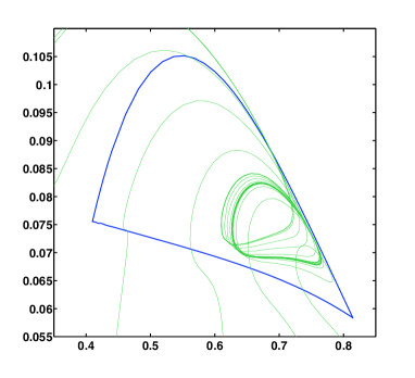
In order to prove attractiveness of the ergodic set, we shall use two couples of charts to cover parts of the simplex 𝒮𝒮\mathcal{S}. The first couple consists in trajectories starting from the boundary of the simplex 𝒮𝒮\partial\mathcal{S}, and driven by constant controls aδ𝑎𝛿a-\delta or A+δ𝐴𝛿A+\delta. The second couple consists in trajectories starting from the line of eigenvectors Φ0subscriptΦ0\Phi_{0}, and driven by constant controls aδ𝑎𝛿a-\delta or A+δ𝐴𝛿A+\delta too.

Refer to caption

(a) Refer to caption(b)

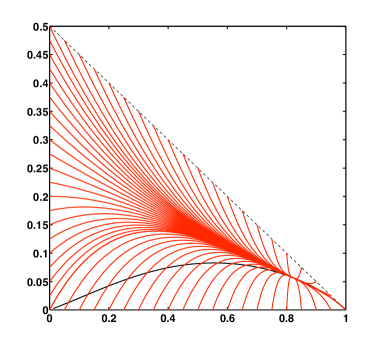
Figure 4: (a) Grid of trajectories starting from the boundary of the simplex 𝒮𝒮\mathcal{S}, with constant control α(t)A+δ𝛼𝑡𝐴𝛿\alpha(t)\equiv A+\delta. (b) Similar figure with constant control α(t)aδ𝛼𝑡𝑎𝛿\alpha(t)\equiv a-\delta.

We shall perform all the computation for one given set of charts (starting from the boundary 𝒮𝒮\partial\mathcal{S} with constant control A+δ𝐴𝛿A+\delta). The other cases are similar. We introduce the following family of curves,

ΓA+δ{sΓ(θ,s)=b(Γ(θ,s),A+δ)Γ(θ,0)=Yθ𝒮,subscriptΓ𝐴𝛿cases𝑠Γ𝜃𝑠𝑏Γ𝜃𝑠𝐴𝛿otherwiseΓ𝜃0subscript𝑌𝜃𝒮otherwise\Gamma_{A+\delta}\begin{cases}\frac{\partial}{\partial s}\Gamma(\theta,s)=b(\Gamma(\theta,s),A+\delta)\\ \Gamma(\theta,0)=Y_{\theta}\in\partial\mathcal{S}\end{cases}\,, (3.10)

where the scalar θ𝜃\theta is a parametrization of the boundary 𝒮𝒮\partial\mathcal{S}. More precisely we adopt a piecewise linear parametrization with the direct orientation. This set of charts covers the whole simplex 𝒮𝒮\mathcal{S}, see Figure 4a.

It is worth recalling that all these trajectories converge towards the eigenvector eA+δsubscript𝑒𝐴𝛿e_{A+\delta} which lies on Φ0subscriptΦ0\Phi_{0}. We denote nA+δ(y)=Θb(y,A+δ)|Θb(y,A+δ)|subscript𝑛𝐴𝛿𝑦Θ𝑏𝑦𝐴𝛿Θ𝑏𝑦𝐴𝛿n_{A+\delta}(y)=\frac{\Theta b(y,A+\delta)}{|\Theta b(y,A+\delta)|} the unitary vector normal to the curve ΓA+δ(θ,)subscriptΓ𝐴𝛿𝜃\Gamma_{A+\delta}(\theta,\cdot) passing through y=ΓA+δ(θ,s)𝒮𝑦subscriptΓ𝐴𝛿𝜃𝑠𝒮y=\Gamma_{A+\delta}(\theta,s)\in\mathcal{S}. We denote ΓA+δ=ΓsubscriptΓ𝐴𝛿Γ\Gamma_{A+\delta}=\Gamma and nA+δ=nsubscript𝑛𝐴𝛿𝑛n_{A+\delta}=n throughout this step.

The key observation is that any trajectory y˙α(t)=b(yα(t),α(t))subscript˙𝑦𝛼𝑡𝑏subscript𝑦𝛼𝑡𝛼𝑡\dot{y}_{\alpha}(t)=b(y_{\alpha}(t),\alpha(t)) is in fact moving monotically along the family of curves {Γ(θ,)}θsubscriptΓ𝜃𝜃\{\Gamma(\theta,\cdot)\}_{\theta} on the sets ΦsubscriptΦ\Phi_{-} and Φ+subscriptΦ\Phi_{+}. We are able to quantify this phenomenon. Let α(t)𝛼𝑡\alpha(t) be any measurable control which takes values in [a,A]𝑎𝐴[a,A]. We have

y˙α(t),n(yα(t))subscript˙𝑦𝛼𝑡𝑛subscript𝑦𝛼𝑡\displaystyle\left\langle\dot{y}_{\alpha}(t),n(y_{\alpha}(t))\right\rangle =(α(t)(A+δ))Fyα(t)+b(yα(t),A+δ),n(yα(t))absent𝛼𝑡𝐴𝛿𝐹subscript𝑦𝛼𝑡𝑏subscript𝑦𝛼𝑡𝐴𝛿𝑛subscript𝑦𝛼𝑡\displaystyle=\left\langle(\alpha(t)-(A+\delta))Fy_{\alpha}(t)+b(y_{\alpha}(t),A+\delta),n(y_{\alpha}(t))\right\rangle
=((A+δ)α(t))|Θb(yα(t),A+δ)|ΘFyα(t),b(yα(t),A+δ)absent𝐴𝛿𝛼𝑡Θ𝑏subscript𝑦𝛼𝑡𝐴𝛿Θ𝐹subscript𝑦𝛼𝑡𝑏subscript𝑦𝛼𝑡𝐴𝛿\displaystyle=\dfrac{((A+\delta)-\alpha(t))}{|\Theta b(y_{\alpha}(t),A+\delta)|}\left\langle\Theta Fy_{\alpha}(t),b(y_{\alpha}(t),A+\delta)\right\rangle
=((A+δ)α(t))|b(yα(t),A+δ)|φ(yα(t)).absent𝐴𝛿𝛼𝑡𝑏subscript𝑦𝛼𝑡𝐴𝛿𝜑subscript𝑦𝛼𝑡\displaystyle=\dfrac{((A+\delta)-\alpha(t))}{|b(y_{\alpha}(t),A+\delta)|}\varphi(y_{\alpha}(t))\,.

We rewrite yα(t)subscript𝑦𝛼𝑡y_{\alpha}(t) using the local chart yα(t)=Γ(θ(t),s(t))subscript𝑦𝛼𝑡Γ𝜃𝑡𝑠𝑡y_{\alpha}(t)=\Gamma(\theta(t),s(t)). We have accordingly,

y˙α(t)=θ˙(t)θΓ(θ(t),s(t))+s˙(t)sΓ(θ(t),s(t)).subscript˙𝑦𝛼𝑡˙𝜃𝑡𝜃Γ𝜃𝑡𝑠𝑡˙𝑠𝑡𝑠Γ𝜃𝑡𝑠𝑡\dot{y}_{\alpha}(t)=\dot{\theta}(t)\dfrac{\partial}{\partial\theta}\Gamma(\theta(t),s(t))+\dot{s}(t)\frac{\partial}{\partial s}\Gamma(\theta(t),s(t))\,.

By construction, we have sΓ(θ,s)=b(Γ(θ,s),A+δ)𝑠Γ𝜃𝑠𝑏Γ𝜃𝑠𝐴𝛿\frac{\partial}{\partial s}\Gamma(\theta,s)=b(\Gamma(\theta,s),A+\delta). Consequently,

y˙α(t),n(yα(t)=θ˙(t)θΓ(θ(t),s(t)),n(Γ(θ(t),s(t)))+0.\left\langle\dot{y}_{\alpha}(t),n(y_{\alpha}(t)\right\rangle=\dot{\theta}(t)\left\langle\dfrac{\partial}{\partial\theta}\Gamma(\theta(t),s(t)),n(\Gamma(\theta(t),s(t)))\right\rangle+0\,.

We compute the evolution of the quantity Γθ,n(Γ)Γ𝜃𝑛Γ\langle\frac{\partial\Gamma}{\partial\theta},n(\Gamma)\rangle along the curve Γ(θ,)Γ𝜃\Gamma(\theta,\cdot). We aim at showing that this quantity has constant sign. This is intuitively clear, since trajectories cannot cross. We make it quantitative in the following calculation. For the sake of clarity, we write temporarily b(Γ,A+δ)=b(Γ)𝑏Γ𝐴𝛿𝑏Γb(\Gamma,A+\delta)=b(\Gamma).

sΓθ,n(Γ)𝑠Γ𝜃𝑛Γ\displaystyle\frac{\partial}{\partial s}\left\langle\frac{\partial\Gamma}{\partial\theta},n(\Gamma)\right\rangle =2Γθs,n(Γ)+Γθ,ΘDb(Γ)ΓsΓθ,n(Γ)n(Γ),1|Θb|ΘDb(Γ)Γsabsentsuperscript2Γ𝜃𝑠𝑛ΓΓ𝜃Θ𝐷𝑏ΓΓ𝑠Γ𝜃𝑛Γ𝑛Γ1Θ𝑏Θ𝐷𝑏ΓΓ𝑠\displaystyle=\left\langle\frac{\partial^{2}\Gamma}{\partial\theta\partial s},n(\Gamma)\right\rangle+\left\langle\frac{\partial\Gamma}{\partial\theta},\Theta Db(\Gamma)\frac{\partial\Gamma}{\partial s}\right\rangle-\left\langle\frac{\partial\Gamma}{\partial\theta},n(\Gamma)\right\rangle\left\langle n(\Gamma),\dfrac{1}{|\Theta b|}\Theta Db(\Gamma)\frac{\partial\Gamma}{\partial s}\right\rangle
=Db(Γ)Γθ,n(Γ)+Γθ,ΘDb(Γ)b(Γ)Γθ,n(Γ)n(Γ),ΘDb(Γ)b(Γ)|Θb(Γ)|absent𝐷𝑏ΓΓ𝜃𝑛ΓΓ𝜃Θ𝐷𝑏Γ𝑏ΓΓ𝜃𝑛Γ𝑛ΓΘ𝐷𝑏Γ𝑏ΓΘ𝑏Γ\displaystyle=\left\langle Db(\Gamma)\frac{\partial\Gamma}{\partial\theta},n(\Gamma)\right\rangle+\left\langle\frac{\partial\Gamma}{\partial\theta},\Theta Db(\Gamma)b(\Gamma)\right\rangle-\left\langle\frac{\partial\Gamma}{\partial\theta},n(\Gamma)\right\rangle\left\langle n(\Gamma),\Theta Db(\Gamma)\dfrac{b(\Gamma)}{|\Theta b(\Gamma)|}\right\rangle
=Γθ,[Db(Γ)TΘ+ΘDb(Γ)]b(Γ)|Θb(Γ)|Γθ,n(Γ)n(Γ),ΘDb(Γ)Θ1n(Γ)absentΓ𝜃delimited-[]𝐷𝑏superscriptΓ𝑇ΘΘ𝐷𝑏Γ𝑏ΓΘ𝑏ΓΓ𝜃𝑛Γ𝑛ΓΘ𝐷𝑏ΓsuperscriptΘ1𝑛Γ\displaystyle=\left\langle\frac{\partial\Gamma}{\partial\theta},\left[Db(\Gamma)^{T}\Theta+\Theta Db(\Gamma)\right]\dfrac{b(\Gamma)}{|\Theta b(\Gamma)|}\right\rangle-\left\langle\frac{\partial\Gamma}{\partial\theta},n(\Gamma)\right\rangle\left\langle n(\Gamma),\Theta Db(\Gamma)\Theta^{-1}n(\Gamma)\right\rangle

Notice that the matrix [Db(Γ)TΘ+ΘDb(Γ)]delimited-[]𝐷𝑏superscriptΓ𝑇ΘΘ𝐷𝑏Γ[Db(\Gamma)^{T}\Theta+\Theta Db(\Gamma)] is everywhere skew-symmetric, so is the matrix ΘΘ\Theta:

[Db(Γ)TΘ+ΘDb(Γ)]T=ΘDb(Γ)Db(Γ)TΘ.superscriptdelimited-[]𝐷𝑏superscriptΓ𝑇ΘΘ𝐷𝑏Γ𝑇Θ𝐷𝑏Γ𝐷𝑏superscriptΓ𝑇Θ\left[Db(\Gamma)^{T}\Theta+\Theta Db(\Gamma)\right]^{T}=-\Theta Db(\Gamma)-Db(\Gamma)^{T}\Theta\,.

Therefore it is equal to ΘΘ\Theta up to a scalar factor:

[Db(Γ)TΘ+ΘDb(Γ)]=ω~(θ,s)Θ.delimited-[]𝐷𝑏superscriptΓ𝑇ΘΘ𝐷𝑏Γ~𝜔𝜃𝑠Θ\left[Db(\Gamma)^{T}\Theta+\Theta Db(\Gamma)\right]=\widetilde{\omega}(\theta,s)\Theta\,.

To conclude, the scalar product Γθ,n(Γ)Γ𝜃𝑛Γ\langle\frac{\partial\Gamma}{\partial\theta},n(\Gamma)\rangle cannot vanish. In addition, we have the semi-explicit formula:

Γθ,n(Γ)=exp(0sω(θ,s)𝑑s)ddθYθ,n(Yθ),Γ𝜃𝑛Γsuperscriptsubscript0𝑠𝜔𝜃superscript𝑠differential-dsuperscript𝑠𝑑𝑑𝜃subscript𝑌𝜃𝑛subscript𝑌𝜃\left\langle\frac{\partial\Gamma}{\partial\theta},n(\Gamma)\right\rangle=\exp\left(\int_{0}^{s}\omega(\theta,s^{\prime})\,ds^{\prime}\right)\left\langle\dfrac{d}{d\theta}Y_{\theta},n(Y_{\theta})\right\rangle\,,

where the scalar ω𝜔\omega is given by

ω𝜔\displaystyle\omega =ω~n(Γ),ΘDb(Γ)Θ1n(Γ)absent~𝜔𝑛ΓΘ𝐷𝑏ΓsuperscriptΘ1𝑛Γ\displaystyle=\widetilde{\omega}-\left\langle n(\Gamma),\Theta Db(\Gamma)\Theta^{-1}n(\Gamma)\right\rangle
=n(Γ),ω~n(Γ)n(Γ),ΘDb(Γ)Θ1n(Γ)absent𝑛Γ~𝜔𝑛Γ𝑛ΓΘ𝐷𝑏ΓsuperscriptΘ1𝑛Γ\displaystyle=\left\langle n(\Gamma),\widetilde{\omega}n(\Gamma)\right\rangle-\left\langle n(\Gamma),\Theta Db(\Gamma)\Theta^{-1}n(\Gamma)\right\rangle
=n(Γ),[Db(Γ)T+ΘDb(Γ)Θ1]n(Γ)n(Γ),ΘDb(Γ)Θ1n(Γ)absent𝑛Γdelimited-[]𝐷𝑏superscriptΓ𝑇Θ𝐷𝑏ΓsuperscriptΘ1𝑛Γ𝑛ΓΘ𝐷𝑏ΓsuperscriptΘ1𝑛Γ\displaystyle=\left\langle n(\Gamma),\left[Db(\Gamma)^{T}+\Theta Db(\Gamma)\Theta^{-1}\right]n(\Gamma)\right\rangle-\left\langle n(\Gamma),\Theta Db(\Gamma)\Theta^{-1}n(\Gamma)\right\rangle
=n(Γ),Db(Γ)Tn(Γ).absent𝑛Γ𝐷𝑏superscriptΓ𝑇𝑛Γ\displaystyle=\left\langle n(\Gamma),Db(\Gamma)^{T}n(\Gamma)\right\rangle\,.

To conclude, we have proven the following Lemma.

Lemma 3.9 (A monotonicity formula).

Let (θA+δ,sA+δ)subscript𝜃𝐴𝛿subscript𝑠𝐴𝛿(\theta_{A+\delta},s_{A+\delta}) be some parametrization of the simplex, given by (3.10). The evolution of θA+δsubscript𝜃𝐴𝛿\theta_{A+\delta} along the trajectories of y˙α(t)=b(yα(t),α(t))subscript˙𝑦𝛼𝑡𝑏subscript𝑦𝛼𝑡𝛼𝑡\dot{y}_{\alpha}(t)=b(y_{\alpha}(t),\alpha(t)) is given by the following formula:

θ˙A+δ(t)=((A+δ)α(t))φ(yα(t))exp(0s(t)ω(θ,s)𝑑s)ddθYθ,nA+δ(Yθ)1,subscript˙𝜃𝐴𝛿𝑡𝐴𝛿𝛼𝑡𝜑subscript𝑦𝛼𝑡superscriptsubscript0𝑠𝑡𝜔𝜃superscript𝑠differential-dsuperscript𝑠superscript𝑑𝑑𝜃subscript𝑌𝜃subscript𝑛𝐴𝛿subscript𝑌𝜃1\dot{\theta}_{A+\delta}(t)=((A+\delta)-\alpha(t))\varphi(y_{\alpha}(t))\exp\left(-\int_{0}^{s(t)}\omega(\theta,s^{\prime})\,ds^{\prime}\right)\left\langle\frac{d}{d\theta}Y_{\theta},n_{A+\delta}(Y_{\theta})\right\rangle^{-1}\,,

where the scalar ω𝜔\omega is defined by

ω(θ,s)=Dyb(Γ(θ,s),A+δ)n(Γ(θ,s)),n(Γ(θ,s)).𝜔𝜃𝑠subscript𝐷𝑦𝑏Γ𝜃𝑠𝐴𝛿𝑛Γ𝜃𝑠𝑛Γ𝜃𝑠\omega(\theta,s)=\left\langle D_{y}b(\Gamma(\theta,s),A+\delta)n(\Gamma(\theta,s)),n(\Gamma(\theta,s))\right\rangle\,.

In particular ω𝜔\omega is uniformly bounded: ωDybsubscriptnorm𝜔subscriptnormsubscript𝐷𝑦𝑏\|\omega\|_{\infty}\leq\|D_{y}b\|_{\infty}.

We build the same chart (θaδ,saδ)subscript𝜃𝑎𝛿subscript𝑠𝑎𝛿(\theta_{a-\delta},s_{a-\delta}) with the constant control α(t)aδ𝛼𝑡𝑎𝛿\alpha(t)\equiv a-\delta,

Γaδ{sΓ(θ,s)=b(Γ(θ,s),aδ)Γ(θ,0)=Yθ𝒮.subscriptΓ𝑎𝛿cases𝑠Γ𝜃𝑠𝑏Γ𝜃𝑠𝑎𝛿otherwiseΓ𝜃0subscript𝑌𝜃𝒮otherwise\Gamma_{a-\delta}\begin{cases}\frac{\partial}{\partial s}\Gamma(\theta,s)=b(\Gamma(\theta,s),a-\delta)\\ \Gamma(\theta,0)=Y_{\theta}\in\partial\mathcal{S}\end{cases}\,. (3.11)

We have similarly

θ˙aδ(t)=((aδ)α(t))φ(yα(t))exp(0s(t)ω(θ,s)𝑑s)ddθYθ,naδ(Yθ)1.subscript˙𝜃𝑎𝛿𝑡𝑎𝛿𝛼𝑡𝜑subscript𝑦𝛼𝑡superscriptsubscript0𝑠𝑡𝜔𝜃superscript𝑠differential-dsuperscript𝑠superscript𝑑𝑑𝜃subscript𝑌𝜃subscript𝑛𝑎𝛿subscript𝑌𝜃1\dot{\theta}_{a-\delta}(t)=((a-\delta)-\alpha(t))\varphi(y_{\alpha}(t))\exp\left(-\int_{0}^{s(t)}\omega(\theta,s^{\prime})\,ds^{\prime}\right)\left\langle\frac{d}{d\theta}Y_{\theta},n_{a-\delta}(Y_{\theta})\right\rangle^{-1}\,.

We recall that we adopt a piecewise linear parametrization with the direct orientation for the boundary 𝒮𝒮\partial\mathcal{S}. Since the fields b(y,α)𝑏𝑦𝛼b(y,\alpha) are all pointing inward the simplex 𝒮𝒮\mathcal{S}, this guarantees that we have in both cases (A+δ𝐴𝛿A+\delta and aδ𝑎𝛿a-\delta),

θddθYθ,n(Yθ)0.for-all𝜃𝑑𝑑𝜃subscript𝑌𝜃𝑛subscript𝑌𝜃0\forall\theta\quad\left\langle\dfrac{d}{d\theta}Y_{\theta},n(Y_{\theta})\right\rangle\leq 0\,.
Refer to caption

(a) Refer to caption(b)

Figure 5: Tunneling effect: the trajectories are trapped in the areas delimited by the green curves. They are forced to enter the approximated ergodic set 𝒵+δsubscript𝒵𝛿\mathcal{Z}_{+\delta} due to the monotonicity formulas (3.13)-(3.14). (a) The set 𝒯Φsubscript𝒯subscriptΦ\mathcal{T}_{-}\subset\Phi_{-}; (b) The set 𝒯+Φ+subscript𝒯subscriptΦ\mathcal{T}_{+}\subset\Phi_{+}.

Similarly we build the second couple of charts, defined through the following families of curves, parametrized by the starting point eβΦ0subscript𝑒𝛽subscriptΦ0e_{\beta}\in\Phi_{0}, see Figure 5,

ΓA+δ{sΓ(β,s)=b(Γ(β,s),A+δ)Γ(β,0)=eβΦ0,Γaδ{sΓ(β,s)=b(Γ(β,s),aδ)Γ(β,0)=eβΦ0.subscriptΓ𝐴𝛿cases𝑠Γ𝛽𝑠𝑏Γ𝛽𝑠𝐴𝛿otherwiseΓ𝛽0subscript𝑒𝛽subscriptΦ0otherwisesubscriptΓ𝑎𝛿cases𝑠Γ𝛽𝑠𝑏Γ𝛽𝑠𝑎𝛿otherwiseΓ𝛽0subscript𝑒𝛽subscriptΦ0otherwise\Gamma_{A+\delta}\begin{cases}\frac{\partial}{\partial s}\Gamma(\beta,s)=b(\Gamma(\beta,s),A+\delta)\\ \Gamma(\beta,0)=e_{\beta}\in\Phi_{0}\end{cases}\,,\quad\Gamma_{a-\delta}\begin{cases}\frac{\partial}{\partial s}\Gamma(\beta,s)=b(\Gamma(\beta,s),a-\delta)\\ \Gamma(\beta,0)=e_{\beta}\in\Phi_{0}\end{cases}\,. (3.12)

We obtain as in Lemma 3.9,

β˙A+δ(t)subscript˙𝛽𝐴𝛿𝑡\displaystyle\dot{\beta}_{A+\delta}(t) =((A+δ)α(t))φ(yα(t))exp(0s(t)ω(β,s)𝑑s)ddβeβ,nA+δ(eβ)1,absent𝐴𝛿𝛼𝑡𝜑subscript𝑦𝛼𝑡superscriptsubscript0𝑠𝑡𝜔𝛽superscript𝑠differential-dsuperscript𝑠superscript𝑑𝑑𝛽subscript𝑒𝛽subscript𝑛𝐴𝛿subscript𝑒𝛽1\displaystyle=((A+\delta)-\alpha(t))\varphi(y_{\alpha}(t))\exp\left(-\int_{0}^{s(t)}\omega(\beta,s^{\prime})\,ds^{\prime}\right)\left\langle\frac{d}{d\beta}e_{\beta},n_{A+\delta}(e_{\beta})\right\rangle^{-1}\,, (3.13)
β˙aδ(t)subscript˙𝛽𝑎𝛿𝑡\displaystyle\dot{\beta}_{a-\delta}(t) =((aδ)α(t))φ(yα(t))exp(0s(t)ω(β,s)𝑑s)ddβeβ,naδ(eβ)1.absent𝑎𝛿𝛼𝑡𝜑subscript𝑦𝛼𝑡superscriptsubscript0𝑠𝑡𝜔𝛽superscript𝑠differential-dsuperscript𝑠superscript𝑑𝑑𝛽subscript𝑒𝛽subscript𝑛𝑎𝛿subscript𝑒𝛽1\displaystyle=((a-\delta)-\alpha(t))\varphi(y_{\alpha}(t))\exp\left(-\int_{0}^{s(t)}\omega(\beta,s^{\prime})\,ds^{\prime}\right)\left\langle\frac{d}{d\beta}e_{\beta},n_{a-\delta}(e_{\beta})\right\rangle^{-1}\,. (3.14)

In this case, we have b(eβ,A+δ)=((A+δ)β)Feβ𝑏subscript𝑒𝛽𝐴𝛿𝐴𝛿𝛽𝐹subscript𝑒𝛽b(e_{\beta},A+\delta)=((A+\delta)-\beta)Fe_{\beta}. Therefore,

βddβeβ,nA+δ(eβ)=sign((A+δ)β)deβdβ,ΘFeβ|ΘFeβ|.for-all𝛽𝑑𝑑𝛽subscript𝑒𝛽subscript𝑛𝐴𝛿subscript𝑒𝛽sign𝐴𝛿𝛽𝑑subscript𝑒𝛽𝑑𝛽Θ𝐹subscript𝑒𝛽Θ𝐹subscript𝑒𝛽\forall\beta\quad\left\langle\dfrac{d}{d\beta}e_{\beta},n_{A+\delta}(e_{\beta})\right\rangle=\mathrm{sign}\,((A+\delta)-\beta)\left\langle\dfrac{de_{\beta}}{d\beta},\dfrac{\Theta Fe_{\beta}}{|\Theta Fe_{\beta}|}\right\rangle\,. (3.15)

Assumption (H4) (3.5) allows to guarantee that this quantity has a constant sign for β<A+δ𝛽𝐴𝛿\beta<A+\delta. Notice that when the charts are defined with the control aδ𝑎𝛿a-\delta, the formula (3.15) is replaced with the following:

βddβeβ,naδ(eβ)=sign((aδ)β)deβdβ,ΘFeβ|ΘFeβ|.for-all𝛽𝑑𝑑𝛽subscript𝑒𝛽subscript𝑛𝑎𝛿subscript𝑒𝛽sign𝑎𝛿𝛽𝑑subscript𝑒𝛽𝑑𝛽Θ𝐹subscript𝑒𝛽Θ𝐹subscript𝑒𝛽\forall\beta\quad\left\langle\dfrac{d}{d\beta}e_{\beta},n_{a-\delta}(e_{\beta})\right\rangle=\mathrm{sign}\,((a-\delta)-\beta)\left\langle\dfrac{de_{\beta}}{d\beta},\dfrac{\Theta Fe_{\beta}}{|\Theta Fe_{\beta}|}\right\rangle\,.

Again this has constant sign for β>aδ𝛽𝑎𝛿\beta>a-\delta. Unfortunately the second set of charts does not cover the whole simplex 𝒮𝒮\mathcal{S} (Figure 5). It is the reason why we introduce the transient set of charts parametrized by Yθ𝒮subscript𝑌𝜃𝒮Y_{\theta}\in\partial\mathcal{S}. We are particularly interested in the two tunnels 𝒯,𝒯+subscript𝒯subscript𝒯\mathcal{T}_{-},\mathcal{T}_{+} defined by the following curves:

  • the subset 𝒯subscript𝒯\mathcal{T}_{-} is defined by its boundary made of 3 pieces (Figure 5a): the trajectory starting from the corner e0=(0 0 1/3)subscript𝑒00013e_{0}=(0\;0\;1/3) with constant control A+δ𝐴𝛿A+\delta; the portion of Φ0subscriptΦ0\Phi_{0} from e0subscript𝑒0e_{0} to eaδsubscript𝑒𝑎𝛿e_{a-\delta}; and the trajectory starting from eaδsubscript𝑒𝑎𝛿e_{a-\delta} with constant control A+δ𝐴𝛿A+\delta. We have 𝒯Φsubscript𝒯subscriptΦ\mathcal{T}_{-}\subset\Phi_{-},

  • the subset 𝒯+subscript𝒯\mathcal{T}_{+} is defined similarly (Figure 5b): it is enclosed by the trajectory starting from the corner e=(1 0 0)subscript𝑒100e_{\infty}=(1\;0\;0) with constant control aδ𝑎𝛿a-\delta; the portion of Φ0subscriptΦ0\Phi_{0} from esubscript𝑒e_{\infty} to eA+δsubscript𝑒𝐴𝛿e_{A+\delta}; and the trajectory starting from eA+δsubscript𝑒𝐴𝛿e_{A+\delta} with constant control aδ𝑎𝛿a-\delta. We have 𝒯+Φ+subscript𝒯subscriptΦ\mathcal{T}_{+}\subset\Phi_{+}.

By comparison arguments we get easily that the second set of charts covers the tunnel 𝒯subscript𝒯\mathcal{T}_{-} (resp. 𝒯+subscript𝒯\mathcal{T}_{+}) with the constant control A+δ𝐴𝛿A+\delta (resp. aδ𝑎𝛿a-\delta). The main feature of these two tunnels is the following: due to Hypothesis (H4) (3.5) and Lemma 3.9, any trajectory that enters one of these tunnels can exit only by entering 𝒵+δsubscript𝒵𝛿\mathcal{Z}_{+\delta}. Moreover it follows monotonically the parametrization of the second chart (3.13)-(3.14). This enables to prove that the trajectory eventually reaches the end of the tunnel: the ergodic set.

Step 5- Attractiveness of the ergodic set.
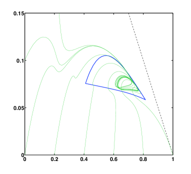
Refer to caption

(a) Refer to caption(b)

Figure 6: Attractiveness and stability of the ergodic set 𝒵0subscript𝒵0\mathcal{Z}_{0}. Several trajectories with arbitrary control α(t)𝛼𝑡\alpha(t) (here, periodic) have been plotted. They all enter the ergodic set and stay there. The right figure is a zoom of the left one.

We state the main result of this step: attractiveness of the approximated ergodic set 𝒵+2δsubscript𝒵2𝛿\mathcal{Z}_{+2\delta}.

Lemma 3.10.

The set 𝒵+2δsubscript𝒵2𝛿\mathcal{Z}_{+2\delta} is attractive: any trajectory yα(t)subscript𝑦𝛼𝑡y_{\alpha}(t) enters the set 𝒵+2δsubscript𝒵2𝛿\mathcal{Z}_{+2\delta} after finite time, at most T0(δ)subscript𝑇0𝛿T_{0}(\delta). The maximal time T0(δ)subscript𝑇0𝛿T_{0}(\delta) does not depend on ϵitalic-ϵ\epsilon.

As this property holds true for any δ>0𝛿0\delta>0 we can conclude that the set 𝒵0subscript𝒵0\mathcal{Z}_{0} is approximately attractive, but we get no estimate about the maximal time T0(δ)subscript𝑇0𝛿T_{0}(\delta) as δ0𝛿0\delta\to 0. In fact we will prove in the next step that close-to-optimal trajectories enter the ergodic set 𝒵0subscript𝒵0\mathcal{Z}_{0} (and even the smaller set 𝒵δsubscript𝒵𝛿\mathcal{Z}_{-\delta}) in finite time: this is a stronger property. The attractiveness property is illustrated in Figure 6: trajectories necessarily enter the set 𝒵+2δsubscript𝒵2𝛿\mathcal{Z}_{+2\delta}.

Proof.

Let yα(t)subscript𝑦𝛼𝑡y_{\alpha}(t) be any trajectory of the system y˙α(t)=b(yα(t),α(t))subscript˙𝑦𝛼𝑡𝑏subscript𝑦𝛼𝑡𝛼𝑡\dot{y}_{\alpha}(t)=b(y_{\alpha}(t),\alpha(t)), where the control α(t)𝛼𝑡\alpha(t) takes values in [a,A]𝑎𝐴[a,A]. We assume without loss of generality that yα(0)Φ+𝒵+2δsubscript𝑦𝛼0subscriptΦsubscript𝒵2𝛿y_{\alpha}(0)\in\Phi_{+}\setminus\mathcal{Z}_{+2\delta}. We define t0subscript𝑡0t_{0} as the first exit time:

t0=inft{t|yα(t)Φ+𝒵+2δ}.subscript𝑡0subscriptinfimum𝑡conditional-set𝑡subscript𝑦𝛼𝑡subscriptΦsubscript𝒵2𝛿t_{0}=\inf_{t}\left\{t\;|\;y_{\alpha}(t)\notin\Phi_{+}\setminus\mathcal{Z}_{+2\delta}\right\}\,.

We face the following alternative: either yα(0)𝒯+subscript𝑦𝛼0subscript𝒯y_{\alpha}(0)\notin\mathcal{T}_{+} then we shall use the first set of charts parametrized by Yθ𝒮subscript𝑌𝜃𝒮Y_{\theta}\in\partial\mathcal{S} (3.11), or yα(0)𝒯+subscript𝑦𝛼0subscript𝒯y_{\alpha}(0)\in\mathcal{T}_{+} then we shall use the second set of charts parametrized by eβΦ0subscript𝑒𝛽subscriptΦ0e_{\beta}\in\Phi_{0} (3.12). We begin with the latter case.

The only way to exit the tunnel 𝒯+subscript𝒯\mathcal{T}_{+} is to enter the set 𝒵+δ𝒵+2δsubscript𝒵𝛿subscript𝒵2𝛿\mathcal{Z}_{+\delta}\subset\mathcal{Z}_{+2\delta}. The quantity βaδ(t)subscript𝛽𝑎𝛿𝑡\beta_{a-\delta}(t) is monotonic. More precisely we have

t[0,t0)β˙aδ(t)δφ(yα(t))exp(s(t)Dyb)|deβdβ,ΘFeβ|ΘFeβ||1.formulae-sequencefor-all𝑡0subscript𝑡0subscript˙𝛽𝑎𝛿𝑡𝛿𝜑subscript𝑦𝛼𝑡𝑠𝑡subscriptnormsubscript𝐷𝑦𝑏superscript𝑑subscript𝑒𝛽𝑑𝛽Θ𝐹subscript𝑒𝛽Θ𝐹subscript𝑒𝛽1\forall t\in[0,t_{0})\quad\dot{\beta}_{a-\delta}(t)\leq-\delta\varphi(y_{\alpha}(t))\exp\left(-s(t)\|D_{y}b\|_{\infty}\right)\left|\left\langle\frac{de_{\beta}}{d\beta},\dfrac{\Theta Fe_{\beta}}{|\Theta Fe_{\beta}|}\right\rangle\right|^{-1}\,.

Recall that the time s(t)𝑠𝑡s(t) is given by the parametrization of the trajectory yα(t)=Γaδ(βaδ(t),s(t))subscript𝑦𝛼𝑡subscriptΓ𝑎𝛿subscript𝛽𝑎𝛿𝑡𝑠𝑡y_{\alpha}(t)=\Gamma_{a-\delta}(\beta_{a-\delta}(t),s(t)). Hence s(t)𝑠𝑡s(t) is uniformly bounded on Φ+𝒵+2δsubscriptΦsubscript𝒵2𝛿\Phi_{+}\setminus\mathcal{Z}_{+2\delta}. This is the reason why we use the set 𝒵+2δsubscript𝒵2𝛿\mathcal{Z}_{+2\delta} rather than the set 𝒵+δsubscript𝒵𝛿\mathcal{Z}_{+\delta} for which we could have s(t)+𝑠𝑡s(t)\to+\infty because eaδ𝒵+δsubscript𝑒𝑎𝛿subscript𝒵𝛿e_{a-\delta}\in\partial\mathcal{Z}_{+\delta}. Therefore the r.h.s of (3.18) can vanish only when yαsubscript𝑦𝛼y_{\alpha} gets close to the set Φ0subscriptΦ0\Phi_{0}. Indeed the factor |deβdβ,ΘFeβ|ΘFeβ||1superscript𝑑subscript𝑒𝛽𝑑𝛽Θ𝐹subscript𝑒𝛽Θ𝐹subscript𝑒𝛽1\left|\left\langle\frac{de_{\beta}}{d\beta},\frac{\Theta Fe_{\beta}}{|\Theta Fe_{\beta}|}\right\rangle\right|^{-1} is clearly bounded from below since |deβdβ,ΘFeβ|ΘFeβ||𝑑subscript𝑒𝛽𝑑𝛽Θ𝐹subscript𝑒𝛽Θ𝐹subscript𝑒𝛽\left|\left\langle\frac{de_{\beta}}{d\beta},\frac{\Theta Fe_{\beta}}{|\Theta Fe_{\beta}|}\right\rangle\right| is bounded from above.

We have a precise description of the dynamics close to Φ0subscriptΦ0\Phi_{0}:

ddtφ(yα(t))𝑑𝑑𝑡𝜑subscript𝑦𝛼𝑡\displaystyle\dfrac{d}{dt}\varphi(y_{\alpha}(t)) =y˙α(t),φ(yα(t))absentsubscript˙𝑦𝛼𝑡𝜑subscript𝑦𝛼𝑡\displaystyle=\left\langle\dot{y}_{\alpha}(t),\nabla\varphi(y_{\alpha}(t))\right\rangle
=b(yα(t),α(t)),φ(yα(t))absent𝑏subscript𝑦𝛼𝑡𝛼𝑡𝜑subscript𝑦𝛼𝑡\displaystyle=\left\langle b(y_{\alpha}(t),\alpha(t)),\nabla\varphi(y_{\alpha}(t))\right\rangle
=b(eβ,α(t)),φ(eβ)+o(|yα(t)eβ|)absent𝑏subscript𝑒𝛽𝛼𝑡𝜑subscript𝑒𝛽𝑜subscript𝑦𝛼𝑡subscript𝑒𝛽\displaystyle=\left\langle b(e_{\beta},\alpha(t)),\nabla\varphi(e_{\beta})\right\rangle+o(|y_{\alpha}(t)-e_{\beta}|) (3.16)
=(α(t)β)Feβ,φ(eβ)+o(|yα(t)eβ|).absent𝛼𝑡𝛽𝐹subscript𝑒𝛽𝜑subscript𝑒𝛽𝑜subscript𝑦𝛼𝑡subscript𝑒𝛽\displaystyle=(\alpha(t)-\beta)\left\langle Fe_{\beta},\nabla\varphi(e_{\beta})\right\rangle+o(|y_{\alpha}(t)-e_{\beta}|)\,.

Hypothesis (H4) guarantees that the quantity Feβ,φ(eβ)𝐹subscript𝑒𝛽𝜑subscript𝑒𝛽\left\langle Fe_{\beta},\nabla\varphi(e_{\beta})\right\rangle is negative for all finite β𝛽\beta:

β<+Feβ,φ(eβ)=Feβ,χβΘdeβdβ=χβΘFeβ,deβdβ<0,formulae-sequencefor-all𝛽𝐹subscript𝑒𝛽𝜑subscript𝑒𝛽𝐹subscript𝑒𝛽subscript𝜒𝛽Θ𝑑subscript𝑒𝛽𝑑𝛽subscript𝜒𝛽Θ𝐹subscript𝑒𝛽𝑑subscript𝑒𝛽𝑑𝛽0\forall\beta<+\infty\quad\left\langle Fe_{\beta},\nabla\varphi(e_{\beta})\right\rangle=\left\langle Fe_{\beta},-\chi_{\beta}\Theta\dfrac{de_{\beta}}{d\beta}\right\rangle=\chi_{\beta}\left\langle\Theta Fe_{\beta},\dfrac{de_{\beta}}{d\beta}\right\rangle<0\,,

where χβsubscript𝜒𝛽\chi_{\beta} is a positive scalar (coming from the discrepancy between the two vectors pointing in the normal direction to Φ0subscriptΦ0\Phi_{0}: φ(eβ)𝜑subscript𝑒𝛽\nabla\varphi(e_{\beta}) and ΘdeβdβΘ𝑑subscript𝑒𝛽𝑑𝛽-\Theta\frac{de_{\beta}}{d\beta}). Unfortunately b(e,α(t)),φ(e)𝑏subscript𝑒𝛼𝑡𝜑subscript𝑒\left\langle b(e_{\infty},\alpha(t)),\nabla\varphi(e_{\infty})\right\rangle may vanish (it is actually the case for the running example: the field b(e,α)𝑏subscript𝑒𝛼b(e_{\infty},\alpha) is independent of α𝛼\alpha and it is tangent to Φ0subscriptΦ0\Phi_{0}). Therefore we have to isolate the large parameters β1much-greater-than𝛽1\beta\gg 1 (trajectory starting close to esubscript𝑒e_{\infty}). To circumvent this issue we investigate the behaviour of yα(t)subscript𝑦𝛼𝑡y_{\alpha}(t) in the neighbourhood of esubscript𝑒e_{\infty}, say a ball (e,η)subscript𝑒superscript𝜂\mathcal{B}(e_{\infty},\eta^{\prime}). We have the following linearization around esubscript𝑒e_{\infty},

b(y,α)=b(e,α)+o(|ye|)=Ge+o(η),𝑏𝑦𝛼𝑏subscript𝑒𝛼𝑜𝑦subscript𝑒𝐺subscript𝑒𝑜superscript𝜂b(y,\alpha)=b(e_{\infty},\alpha)+o(|y-e_{\infty}|)=Ge_{\infty}+o(\eta^{\prime})\,, (3.17)

since Fe=0𝐹subscript𝑒0Fe_{\infty}=0 (see Hypothesis (H2) and subsequent discussion). Moreover we have Ge0𝐺subscript𝑒0Ge_{\infty}\neq 0 (see Hypothesis (H3) and subsequent discussion). The linearization is uniform with respect to α[a,A]𝛼𝑎𝐴\alpha\in[a,A]. Therefore the trajectory is pushed away from esubscript𝑒e_{\infty} in finite time, uniformly with respect to the initial data yα(0)(e,η)subscript𝑦𝛼0subscript𝑒superscript𝜂y_{\alpha}(0)\in\mathcal{B}(e_{\infty},\eta^{\prime}).

We choose η>0superscript𝜂0\eta^{\prime}>0 such that the higher-order terms in the linearization (3.17) are negligible in front of Ge𝐺subscript𝑒Ge_{\infty}. We choose the largest possible B𝐵B such that the portion {eβ:βB}(e,η)conditional-setsubscript𝑒𝛽𝛽𝐵subscript𝑒superscript𝜂\{e_{\beta}:\beta\geq B\}\subset\mathcal{B}(e_{\infty},\eta^{\prime}). There exists ν>0𝜈0\nu>0 depending on B𝐵B such that the following inequality holds,

βBFeβ,φ(eβ)>ν>0.formulae-sequencefor-all𝛽𝐵𝐹subscript𝑒𝛽𝜑subscript𝑒𝛽𝜈0\forall\beta\leq B\quad-\left\langle Fe_{\beta},\nabla\varphi(e_{\beta})\right\rangle>\nu>0\,.

Accordingly we choose a small δ>0superscript𝛿0\delta^{\prime}>0 such that the error term in the linearization (3.16) is uniformly smaller than δν𝛿𝜈\delta\nu for |yα(t)eβ|<δsubscript𝑦𝛼𝑡subscript𝑒𝛽superscript𝛿|y_{\alpha}(t)-e_{\beta}|<\delta^{\prime} and βB𝛽𝐵\beta\leq B. Thus we have

t[0,t0)ddtφ(yα(t))2δνδν=δν.formulae-sequencefor-all𝑡0subscript𝑡0𝑑𝑑𝑡𝜑subscript𝑦𝛼𝑡2𝛿𝜈𝛿𝜈𝛿𝜈\forall t\in[0,t_{0})\quad\dfrac{d}{dt}\varphi(y_{\alpha}(t))\geq 2\delta\nu-\delta\nu=\delta\nu\,.

This defines a narrow band of size δsuperscript𝛿\delta^{\prime} around the portion {eβ:A+2δβB}Φ0conditional-setsubscript𝑒𝛽𝐴2𝛿𝛽𝐵subscriptΦ0\{e_{\beta}:A+2\delta\leq\beta\leq B\}\subset\Phi_{0} in which the quantity φ(yα(t))𝜑subscript𝑦𝛼𝑡\varphi(y_{\alpha}(t)) is increasing, uniformly in time. Therefore the trajectory stays away from Φ0subscriptΦ0\Phi_{0}. Consequently the quantity βaδ(t)subscript𝛽𝑎𝛿𝑡\beta_{a-\delta}(t) is decreasing, uniformly in time, and βaδ(t)subscript𝛽𝑎𝛿𝑡\beta_{a-\delta}(t) gets smaller than A+2δ𝐴2𝛿A+2\delta in finite time. This means that yα(t)subscript𝑦𝛼𝑡y_{\alpha}(t) enters 𝒵+2δsubscript𝒵2𝛿\mathcal{Z}_{+2\delta} in finite time when yα(0)𝒯+subscript𝑦𝛼0subscript𝒯y_{\alpha}(0)\in\mathcal{T}_{+}.

We now consider the case yα(0)𝒯+subscript𝑦𝛼0subscript𝒯y_{\alpha}(0)\notin\mathcal{T}_{+}. We choose the parametrization (3.11) given by the charts associated to the constant control aδ𝑎𝛿a-\delta, and the initial point Yθsubscript𝑌𝜃Y_{\theta} lying on 𝒮𝒮\partial\mathcal{S}. From (3.13) we deduce that θaδ(t)subscript𝜃𝑎𝛿𝑡\theta_{a-\delta}(t) is nonincreasing up to t0subscript𝑡0t_{0}:

t[0,t0)θ˙aδ(t)δφ(yα(t))exp(s(t)Dyb)|ddθYθ,naδ(Yθ)|1.formulae-sequencefor-all𝑡0subscript𝑡0subscript˙𝜃𝑎𝛿𝑡𝛿𝜑subscript𝑦𝛼𝑡𝑠𝑡subscriptnormsubscript𝐷𝑦𝑏superscript𝑑𝑑𝜃subscript𝑌𝜃subscript𝑛𝑎𝛿subscript𝑌𝜃1\forall t\in[0,t_{0})\quad\dot{\theta}_{a-\delta}(t)\geq\delta\varphi(y_{\alpha}(t))\exp\left(-s(t)\|D_{y}b\|_{\infty}\right)\left|\left\langle\frac{d}{d\theta}Y_{\theta},n_{a-\delta}(Y_{\theta})\right\rangle\right|^{-1}\,. (3.18)

The function θaδ(t)subscript𝜃𝑎𝛿𝑡\theta_{a-\delta}(t) is naturally bounded for t[0,t0)𝑡0subscript𝑡0t\in[0,t_{0}). In fact, the point Yθsubscript𝑌𝜃Y_{\theta} cannot make a complete turn around the boundary 𝒮𝒮\partial\mathcal{S}. For instance, when Yθ=e0subscript𝑌𝜃subscript𝑒0Y_{\theta}=e_{0}, we have necessarily yα(t)Φsubscript𝑦𝛼𝑡subscriptΦy_{\alpha}(t)\in\Phi_{-}, since the trajectory γaδ0superscriptsubscript𝛾𝑎𝛿0\gamma_{a-\delta}^{0} lies in ΦsubscriptΦ\Phi_{-}. We denote by θ¯¯𝜃\overline{\theta} a bound from above for θaδ(t)subscript𝜃𝑎𝛿𝑡\theta_{a-\delta}(t).

Recall that the time s(t)𝑠𝑡s(t) is uniformly bounded on Φ+𝒵+2δsubscriptΦsubscript𝒵2𝛿\Phi_{+}\setminus\mathcal{Z}_{+2\delta}. As previously the factor |ddθYθ,naδ(Yθ)|1superscript𝑑𝑑𝜃subscript𝑌𝜃subscript𝑛𝑎𝛿subscript𝑌𝜃1\left|\left\langle\frac{d}{d\theta}Y_{\theta},n_{a-\delta}(Y_{\theta})\right\rangle\right|^{-1} is clearly bounded from below since |ddθYθ,naδ(Yθ)|𝑑𝑑𝜃subscript𝑌𝜃subscript𝑛𝑎𝛿subscript𝑌𝜃\left|\left\langle\frac{d}{d\theta}Y_{\theta},n_{a-\delta}(Y_{\theta})\right\rangle\right| is bounded from above.

The descriptions of the dynamics close to Φ0subscriptΦ0\Phi_{0} (3.16) and esubscript𝑒e_{\infty} (3.17) are still valid. From (3.16) we deduce that the following estimate holds true for |yα(t)eβ|<δsubscript𝑦𝛼𝑡subscript𝑒𝛽superscript𝛿|y_{\alpha}(t)-e_{\beta}|<\delta^{\prime} and βa2δ𝛽𝑎2𝛿\beta\leq a-2\delta,

ddtφ(yα(t))2δν+δν=δν.𝑑𝑑𝑡𝜑subscript𝑦𝛼𝑡2𝛿𝜈𝛿𝜈𝛿𝜈\dfrac{d}{dt}\varphi(y_{\alpha}(t))\leq-2\delta\nu+\delta\nu=-\delta\nu\,.

This defines a narrow band of size δsuperscript𝛿\delta^{\prime} around the portion {eβ:0βa2δ}Φ0conditional-setsubscript𝑒𝛽0𝛽𝑎2𝛿subscriptΦ0\{e_{\beta}:0\leq\beta\leq a-2\delta\}\subset\Phi_{0} in which the quantity φ(yα(t))𝜑subscript𝑦𝛼𝑡\varphi(y_{\alpha}(t)) is uniformly decreasing. Once it enters this narrow band, the trajectory necessarily crosses Φ0subscriptΦ0\Phi_{0} in finite time. It leaves Φ+subscriptΦ\Phi_{+} and it enters the tunnel 𝒯subscript𝒯\mathcal{T}_{-}.

On the other hand, we build an analogous narrow band around the portion {eβ:A+2δβ+}Φ0conditional-setsubscript𝑒𝛽𝐴2𝛿𝛽subscriptΦ0\{e_{\beta}:A+2\delta\leq\beta\leq+\infty\}\subset\Phi_{0}. It is the union of the tunnel 𝒯+subscript𝒯\mathcal{T}_{+} and the ball B(e,η)𝐵subscript𝑒superscript𝜂B(e_{\infty},\eta^{\prime}).

If yα(0)subscript𝑦𝛼0y_{\alpha}(0) starts within (e,η)subscript𝑒superscript𝜂\mathcal{B}(e_{\infty},\eta^{\prime}), the trajectory will leave the ball after a finite time of order τ=2|Ge|ηsuperscript𝜏2𝐺subscript𝑒superscript𝜂\tau^{\prime}=2|Ge_{\infty}|\eta^{\prime}. We cannot rule out the fact that it comes back inside the ball several times. Alternatively, we can evaluate the time the trajectory yαsubscript𝑦𝛼y_{\alpha} spends inside the balls (e,η)subscript𝑒superscript𝜂\mathcal{B}(e_{\infty},\eta^{\prime}) and (e,2η)subscript𝑒2superscript𝜂\mathcal{B}(e_{\infty},2\eta^{\prime}) each time it travels through (e,η)subscript𝑒superscript𝜂\mathcal{B}(e_{\infty},\eta^{\prime}). Clearly the trajectory spends a time at most τ=2|Ge|ηsuperscript𝜏2𝐺subscript𝑒superscript𝜂\tau^{\prime}=2|Ge_{\infty}|\eta^{\prime} inside the first ball, and a time at least τsuperscript𝜏\tau^{\prime} in the annulus (e,2η)(e,η)subscript𝑒2superscript𝜂subscript𝑒superscript𝜂\mathcal{B}(e_{\infty},2\eta^{\prime})\setminus\mathcal{B}(e_{\infty},\eta^{\prime}). Outside the narrow bands, the quantity θaδsubscript𝜃𝑎𝛿\theta_{a-\delta} is monotonic with the following estimate:

θ˙aδ(t)cη,subscript˙𝜃𝑎𝛿𝑡subscript𝑐superscript𝜂\dot{\theta}_{a-\delta}(t)\geq c_{\eta^{\prime}}\,,

for some constant cη>0subscript𝑐superscript𝜂0c_{\eta^{\prime}}>0. As a conclusion, if we denote by N𝑁N the number of times the trajectory yαsubscript𝑦𝛼y_{\alpha} travels through (e,η)subscript𝑒superscript𝜂\mathcal{B}(e_{\infty},\eta^{\prime}), we have

θaδ(t0)θaδ(0)N(τ.0+τcη)(e,2η)+(t02Nτ)cηoutside the narrow bands.subscript𝜃𝑎𝛿subscript𝑡0subscript𝜃𝑎𝛿0subscript𝑁superscript𝜏.0superscript𝜏subscript𝑐superscript𝜂subscript𝑒2superscript𝜂subscriptsubscript𝑡02𝑁superscript𝜏subscript𝑐superscript𝜂outside the narrow bands\theta_{a-\delta}(t_{0})-\theta_{a-\delta}(0)\geq\underbrace{N\left(\tau^{\prime}.0+\tau^{\prime}c_{\eta^{\prime}}\right)}_{\mathcal{B}(e_{\infty},2\eta^{\prime})}+\underbrace{(t_{0}-2N\tau^{\prime})c_{\eta^{\prime}}}_{\text{outside the narrow bands}}\,.

Therefore, the number N𝑁N is bounded. Moreover we have Nτθ¯cη𝑁superscript𝜏¯𝜃subscript𝑐superscript𝜂N\tau^{\prime}\leq\frac{\overline{\theta}}{c_{\eta^{\prime}}}. Consequently, the time t0subscript𝑡0t_{0} is also bounded, and we have

t02Nτ+θ¯cη=3θ¯cη.subscript𝑡02𝑁superscript𝜏¯𝜃subscript𝑐superscript𝜂3¯𝜃subscript𝑐superscript𝜂t_{0}\leq 2N\tau^{\prime}+\frac{\overline{\theta}}{c_{\eta^{\prime}}}=3\frac{\overline{\theta}}{c_{\eta^{\prime}}}\,.

We have finally proven that the trajectory yα(t)subscript𝑦𝛼𝑡y_{\alpha}(t) leaves the set Φ+𝒵+2δsubscriptΦsubscript𝒵2𝛿\Phi_{+}\setminus\mathcal{Z}_{+2\delta} after finite time. A precise follow-up of the time spent in this zone shows that it is uniformly bounded with respect to the initial data yα(0)subscript𝑦𝛼0y_{\alpha}(0). We now face the following alternative: either the trajectory enters the set 𝒵+2δsubscript𝒵2𝛿\mathcal{Z}_{+2\delta} at time t0subscript𝑡0t_{0}, or it enters the set Φ𝒵+2δsubscriptΦsubscript𝒵2𝛿\Phi_{-}\setminus\mathcal{Z}_{+2\delta}. In the former case there is nothing more to say. In the latter case, the trajectory crosses the line Φ0subscriptΦ0\Phi_{0}. It does so on the portion {eβ| 0βa2δ}conditional-setsubscript𝑒𝛽 0𝛽𝑎2𝛿\{e_{\beta}\;|\;0\leq\beta\leq a-2\delta\} (otherwise the vector field b(eβ,α(t0))𝑏subscript𝑒𝛽𝛼subscript𝑡0b(e_{\beta},\alpha(t_{0})) points in the wrong direction, from ΦsubscriptΦ\Phi_{-} to Φ+subscriptΦ\Phi_{+}, and the trajectory lies in the tunnel 𝒯+subscript𝒯\mathcal{T}_{+}). We conclude that the trajectory enters the tunnel 𝒯subscript𝒯\mathcal{T}_{-} at t=t0𝑡subscript𝑡0t=t_{0}.

From t=t0𝑡subscript𝑡0t=t_{0} and yα(t0)𝒯subscript𝑦𝛼subscript𝑡0subscript𝒯y_{\alpha}(t_{0})\in\mathcal{T}_{-} we repeat the same procedure as for yα(0)𝒯+subscript𝑦𝛼0subscript𝒯y_{\alpha}(0)\in\mathcal{T}_{+}, except that we change the control determining the charts: we switch from ΓaδsubscriptΓ𝑎𝛿\Gamma_{a-\delta} to ΓA+δsubscriptΓ𝐴𝛿\Gamma_{A+\delta}. Again, the quantity βA+δ(t)subscript𝛽𝐴𝛿𝑡\beta_{A+\delta}(t) is monotonic, and we have

tt0β˙A+δ(t)δ|φ(yα(t))|exp(s(t)Dyb)|deβdβ,ΘFeβ|ΘFeβ||1.formulae-sequencefor-all𝑡subscript𝑡0subscript˙𝛽𝐴𝛿𝑡𝛿𝜑subscript𝑦𝛼𝑡𝑠𝑡subscriptnormsubscript𝐷𝑦𝑏superscript𝑑subscript𝑒𝛽𝑑𝛽Θ𝐹subscript𝑒𝛽Θ𝐹subscript𝑒𝛽1\forall t\geq t_{0}\quad\dot{\beta}_{A+\delta}(t)\geq\delta\left|\varphi(y_{\alpha}(t))\right|\exp\left(-s(t)\|D_{y}b\|_{\infty}\right)\left|\left\langle\frac{de_{\beta}}{d\beta},\dfrac{\Theta Fe_{\beta}}{|\Theta Fe_{\beta}|}\right\rangle\right|^{-1}\,.

This quantity is positive, and we can prove as above that the quantity φ(yα(t))𝜑subscript𝑦𝛼𝑡\varphi(y_{\alpha}(t)) is uniformly decreasing around the portion {eβ:0βa2δ}conditional-setsubscript𝑒𝛽0𝛽𝑎2𝛿\{e_{\beta}:0\leq\beta\leq a-2\delta\}. We deduce as previously that the trajectory necessarily enters the set 𝒵+2δsubscript𝒵2𝛿\mathcal{Z}_{+2\delta} in finite time T0(y)subscript𝑇0𝑦T_{0}(y). The time is uniformly bounded with respect to the trajectory yαsubscript𝑦𝛼y_{\alpha}, independently of ϵitalic-ϵ\epsilon. ∎

Step 6- Close-to-optimal trajectories do not stay close to the boundary of the ergodic set.

Let T0(δ)subscript𝑇0𝛿T_{0}(\delta) be the maximal time of entry in the set 𝒵+2δsubscript𝒵2𝛿\mathcal{Z}_{+2\delta} for the trajectory y˙α(t)=b(yα(t),α(t))subscript˙𝑦𝛼𝑡𝑏subscript𝑦𝛼𝑡𝛼𝑡\dot{y}_{\alpha}(t)=b(y_{\alpha}(t),\alpha(t)). Let us mention that the set 𝒵+2δsubscript𝒵2𝛿\mathcal{Z}_{+2\delta} is stable (The proof is similar to the stability of 𝒵0subscript𝒵0\mathcal{Z}_{0}, see Lemma 3.5).

The final step in the proof of Theorem 3.2 consists in carefully following trajectories running in the layer Δδ=𝒵+2δ𝒵δsubscriptΔ𝛿subscript𝒵2𝛿subscript𝒵𝛿\Delta_{\delta}=\mathcal{Z}_{+2\delta}\setminus\mathcal{Z}_{-\delta}. It is a narrow band surrounding the boundary of the ergodic set 𝒵0subscript𝒵0\partial\mathcal{Z}_{0}. Heuristically, if the trajectory stays in this band forever, then it follows closely the two trajectories defining 𝒵0subscript𝒵0\partial\mathcal{Z}_{0} (3.7). Thus it spends most of the time in the neighbourhood of easubscript𝑒𝑎e_{a} and eAsubscript𝑒𝐴e_{A}, where the reward values are respectively λ(a)𝜆𝑎\lambda(a) and λ(A)𝜆𝐴\lambda(A). From Hypothesis (H2), and particularly λ(α)>max(λ(a),λ(A))𝜆superscript𝛼𝜆𝑎𝜆𝐴\lambda(\alpha^{*})>\max\left(\lambda(a),\lambda(A)\right), we deduce that such a trajectory is far from optimality.

In the next lines we develop this argumentation with quantitative bounds. We will pay much attention to proving that the maximal exit time T1(ϵ,δ)subscript𝑇1italic-ϵ𝛿T_{1}(\epsilon,\delta) outside ΔδsubscriptΔ𝛿\Delta_{\delta} is such that ϵT1(ϵ,δ)1much-less-thanitalic-ϵsubscript𝑇1italic-ϵ𝛿1\epsilon T_{1}(\epsilon,\delta)\ll 1, uniformly.

The width of the narrow band Δδ=𝒵+2δ𝒵δsubscriptΔ𝛿subscript𝒵2𝛿subscript𝒵𝛿\Delta_{\delta}=\mathcal{Z}_{+2\delta}\setminus\mathcal{Z}_{-\delta} is of order δ𝛿\delta. We introduce an intermediate scale η𝜂\eta, with δη1much-less-than𝛿𝜂much-less-than1\delta\ll\eta\ll 1. We denote Ba=B(ea;2η)subscript𝐵𝑎𝐵subscript𝑒𝑎2𝜂B_{a}=B(e_{a};2\eta) and BA=B(eA;2η)subscript𝐵𝐴𝐵subscript𝑒𝐴2𝜂B_{A}=B(e_{A};2\eta) the balls of radius η𝜂\eta with respective centers a,A𝑎𝐴a,A. The scales δ𝛿\delta and η𝜂\eta are to be determined later. Roughly speaking, the scale η𝜂\eta is determined such that ηλ(α)max(λ(a),λ(A))much-less-than𝜂𝜆superscript𝛼𝜆𝑎𝜆𝐴\eta\ll\lambda(\alpha^{*})-\max\left(\lambda(a),\lambda(A)\right), and δ𝛿\delta is adjusted accordingly.

Our claim is the following: if δ𝛿\delta is chosen small enough, then close-to-optimal trajectories cannot stay in ΔδsubscriptΔ𝛿\Delta_{\delta} forever. Let us mention that the set 𝒵δsubscript𝒵𝛿\mathcal{Z}_{-\delta} is not stable. However we require only that the trajectory enters once in 𝒵δsubscript𝒵𝛿\mathcal{Z}_{-\delta} where we can use the uniform controllability Lemma 3.6.

Lemma 3.11.

Let yα(t)subscript𝑦𝛼𝑡y_{\alpha}(t) be a close-to-optimal trajectory in the following sense:

0+eϵtL(yα(t))𝑑tuϵ(y)O(1).superscriptsubscript0superscript𝑒italic-ϵ𝑡𝐿subscript𝑦𝛼𝑡differential-d𝑡subscript𝑢italic-ϵ𝑦𝑂1\int_{0}^{+\infty}e^{-\epsilon t}L(y_{\alpha}(t))\,dt\geq u_{\epsilon}(y)-O(1)\,.

This trajectory must leave the narrow band ΔδsubscriptΔ𝛿\Delta_{\delta} before some maximal time T1(ϵ,δ)subscript𝑇1italic-ϵ𝛿T_{1}(\epsilon,\delta). In addition we have ϵT1(ϵ,δ)=O(η)italic-ϵsubscript𝑇1italic-ϵ𝛿𝑂𝜂\epsilon T_{1}(\epsilon,\delta)=O(\eta) as ϵ0italic-ϵ0\epsilon\to 0, uniformly for y𝒮𝑦𝒮y\in\mathcal{S}.

Proof.

We begin with some considerations about optimality of trajectories. A first important remark is that for all y𝒮𝑦𝒮y\in\mathcal{S} we have lim infϵ0ϵuϵ(y)λ(α)subscriptlimit-infimumitalic-ϵ0italic-ϵsubscript𝑢italic-ϵ𝑦𝜆superscript𝛼\liminf_{\epsilon\to 0}\epsilon u_{\epsilon}(y)\geq\lambda(\alpha^{*}), uniformly in 𝒮𝒮\mathcal{S}. Indeed we may choose the constant value control α(t)α𝛼𝑡superscript𝛼\alpha(t)\equiv\alpha^{*} in the optimization problem (3.3). We know that exponential convergence occurs towards the eigenvector eαsubscript𝑒superscript𝛼e_{\alpha^{*}}:

|yα(t)eα|C|yeα|eμαt,subscript𝑦superscript𝛼𝑡subscript𝑒superscript𝛼𝐶𝑦subscript𝑒superscript𝛼superscript𝑒subscript𝜇superscript𝛼𝑡|y_{\alpha^{*}}(t)-e_{\alpha^{*}}|\leq C|y-e_{\alpha^{*}}|e^{-\mu_{\alpha^{*}}t}\,,

where μαsubscript𝜇superscript𝛼\mu_{\alpha^{*}} is the spectral gap and C𝐶C denotes some absolute constant. This yields the estimate

ϵ0+eϵtL(yα(t))𝑑titalic-ϵsuperscriptsubscript0superscript𝑒italic-ϵ𝑡𝐿subscript𝑦superscript𝛼𝑡differential-d𝑡\displaystyle\epsilon\int_{0}^{+\infty}e^{-\epsilon t}L(y_{\alpha^{*}}(t))\,dt =ϵ0+eϵtL(eα)𝑑t+ϵ0+eϵt(L(yα(t))L(eα))𝑑tabsentitalic-ϵsuperscriptsubscript0superscript𝑒italic-ϵ𝑡𝐿subscript𝑒superscript𝛼differential-d𝑡italic-ϵsuperscriptsubscript0superscript𝑒italic-ϵ𝑡𝐿subscript𝑦superscript𝛼𝑡𝐿subscript𝑒superscript𝛼differential-d𝑡\displaystyle=\epsilon\int_{0}^{+\infty}e^{-\epsilon t}L(e_{\alpha^{*}})\,dt+\epsilon\int_{0}^{+\infty}e^{-\epsilon t}\left(L(y_{\alpha^{*}}(t))-L(e_{\alpha^{*}})\right)\,dt
λ(α)DLϵ0+eϵt|yα(t)eα|𝑑tabsent𝜆superscript𝛼subscriptnorm𝐷𝐿italic-ϵsuperscriptsubscript0superscript𝑒italic-ϵ𝑡subscript𝑦superscript𝛼𝑡subscript𝑒superscript𝛼differential-d𝑡\displaystyle\geq\lambda(\alpha^{*})-\|DL\|_{\infty}\epsilon\int_{0}^{+\infty}e^{-\epsilon t}|y_{\alpha^{*}}(t)-e_{\alpha^{*}}|\,dt
λ(α)CDL|yeα|ϵ0+eϵteμαt𝑑tabsent𝜆superscript𝛼𝐶subscriptnorm𝐷𝐿𝑦subscript𝑒superscript𝛼italic-ϵsuperscriptsubscript0superscript𝑒italic-ϵ𝑡superscript𝑒subscript𝜇superscript𝛼𝑡differential-d𝑡\displaystyle\geq\lambda(\alpha^{*})-C\|DL\|_{\infty}|y-e_{\alpha^{*}}|\epsilon\int_{0}^{+\infty}e^{-\epsilon t}e^{-\mu_{\alpha^{*}}t}\,dt
λ(α)CDLϵϵ+μα.absent𝜆superscript𝛼𝐶subscriptnorm𝐷𝐿italic-ϵitalic-ϵsubscript𝜇superscript𝛼\displaystyle\geq\lambda(\alpha^{*})-C\|DL\|_{\infty}\dfrac{\epsilon}{\epsilon+\mu_{\alpha^{*}}}\,.

By letting ϵ0italic-ϵ0\epsilon\to 0 we deduce the estimate

lim infϵ0ϵuϵ(y)λ(α),uniformly for y𝒮.subscriptlimit-infimumitalic-ϵ0italic-ϵsubscript𝑢italic-ϵ𝑦𝜆superscript𝛼uniformly for y𝒮\liminf_{\epsilon\to 0}\epsilon u_{\epsilon}(y)\geq\lambda(\alpha^{*})\,,\quad\text{uniformly for $y\in\mathcal{S}$}\,. (3.19)

Now we examine the reward of trajectories during their passage in ΔδsubscriptΔ𝛿\Delta_{\delta}. Let yαsubscript𝑦𝛼y_{\alpha} be such that

t(T0(y),T1(y))yα(t)Δδ,formulae-sequencefor-all𝑡subscript𝑇0𝑦subscript𝑇1𝑦subscript𝑦𝛼𝑡subscriptΔ𝛿\forall t\in(T_{0}(y),T_{1}(y))\quad y_{\alpha}(t)\in\Delta_{\delta}\,,

(note that we may a priori have T1(y)=+subscript𝑇1𝑦T_{1}(y)=+\infty). We distinguish between the different parts of ΔδsubscriptΔ𝛿\Delta_{\delta}. Either yα(t)subscript𝑦𝛼𝑡y_{\alpha}(t) belongs to Δδ(BaBA)subscriptΔ𝛿subscript𝐵𝑎subscript𝐵𝐴\Delta_{\delta}\cap(B_{a}\cup B_{A}) or it belongs to the complementary set. We begin with the latter case. We assume that

t(t1,t2)yα(t)Δδ(BaBA).formulae-sequencefor-all𝑡subscript𝑡1subscript𝑡2subscript𝑦𝛼𝑡subscriptΔ𝛿subscript𝐵𝑎subscript𝐵𝐴\forall t\in(t_{1},t_{2})\quad y_{\alpha}(t)\in\Delta_{\delta}\setminus(B_{a}\cup B_{A})\,.

We first prove that, outside the balls Basubscript𝐵𝑎B_{a} and BAsubscript𝐵𝐴B_{A}, yα(t)subscript𝑦𝛼𝑡y_{\alpha}(t) is close to either the curve γasubscript𝛾𝑎\gamma_{a} or the curve γAsubscript𝛾𝐴\gamma_{A}. We deal with the upper part ΔδΦsubscriptΔ𝛿subscriptΦ\Delta_{\delta}\cap\Phi_{-}, where the curve γAsubscript𝛾𝐴\gamma_{A} lies, without loss of generality. We use Lemma 3.9 for this purpose. We recall (3.13) adapted to the constant value control A𝐴A (instead of A+δ)A+\delta):

β˙A(t)(Aα(t))|φ(yα(t))|exp(s(t)Dyb)|deβdβ,ΘFeβ|ΘFeβ||1.subscript˙𝛽𝐴𝑡𝐴𝛼𝑡𝜑subscript𝑦𝛼𝑡𝑠𝑡subscriptnormsubscript𝐷𝑦𝑏superscript𝑑subscript𝑒𝛽𝑑𝛽Θ𝐹subscript𝑒𝛽Θ𝐹subscript𝑒𝛽1\dot{\beta}_{A}(t)\geq(A-\alpha(t))\left|\varphi(y_{\alpha}(t))\right|\exp\left(-s(t)\|D_{y}b\|_{\infty}\right)\left|\left\langle\frac{de_{\beta}}{d\beta},\dfrac{\Theta Fe_{\beta}}{|\Theta Fe_{\beta}|}\right\rangle\right|^{-1}\,.

Outside the balls Basubscript𝐵𝑎B_{a} and BAsubscript𝐵𝐴B_{A}, the time s(t)𝑠𝑡s(t) is uniformly bounded, and |φ|𝜑|\varphi| is bounded from below. We have

|φ(yα(t))|exp(s(t)Dyb)|deβdβ,ΘFeβ|ΘFeβ||1cη,𝜑subscript𝑦𝛼𝑡𝑠𝑡subscriptnormsubscript𝐷𝑦𝑏superscript𝑑subscript𝑒𝛽𝑑𝛽Θ𝐹subscript𝑒𝛽Θ𝐹subscript𝑒𝛽1subscript𝑐𝜂\left|\varphi(y_{\alpha}(t))\right|\exp\left(-s(t)\|D_{y}b\|_{\infty}\right)\left|\left\langle\frac{de_{\beta}}{d\beta},\dfrac{\Theta Fe_{\beta}}{|\Theta Fe_{\beta}|}\right\rangle\right|^{-1}\geq c_{\eta}\,,

for some positive constant cηsubscript𝑐𝜂c_{\eta}. Thus,

cηt1t2(Aα(t))𝑑tβ(t2)β(t1)3δ.subscript𝑐𝜂superscriptsubscriptsubscript𝑡1subscript𝑡2𝐴𝛼𝑡differential-d𝑡𝛽subscript𝑡2𝛽subscript𝑡13𝛿c_{\eta}\int_{t_{1}}^{t_{2}}(A-\alpha(t))\,dt\leq\beta(t_{2})-\beta(t_{1})\leq 3\delta\,.

We deduce that

ddt|γA(t+τ)yα(t)|2𝑑𝑑𝑡superscriptsubscript𝛾𝐴𝑡𝜏subscript𝑦𝛼𝑡2\displaystyle\dfrac{d}{dt}|\gamma_{A}(t+\tau)-y_{\alpha}(t)|^{2} =2b(γA(t+τ),A)b(yα(t),α(t)),γA(t+τ)yα(t)absent2𝑏subscript𝛾𝐴𝑡𝜏𝐴𝑏subscript𝑦𝛼𝑡𝛼𝑡subscript𝛾𝐴𝑡𝜏subscript𝑦𝛼𝑡\displaystyle=2\left\langle b(\gamma_{A}(t+\tau),A)-b(y_{\alpha}(t),\alpha(t)),\gamma_{A}(t+\tau)-y_{\alpha}(t)\right\rangle
=2b(γA(t+τ),α(t))b(yα(t),α(t)),γA(t+τ)yα(t)absent2𝑏subscript𝛾𝐴𝑡𝜏𝛼𝑡𝑏subscript𝑦𝛼𝑡𝛼𝑡subscript𝛾𝐴𝑡𝜏subscript𝑦𝛼𝑡\displaystyle=2\left\langle b(\gamma_{A}(t+\tau),\alpha(t))-b(y_{\alpha}(t),\alpha(t)),\gamma_{A}(t+\tau)-y_{\alpha}(t)\right\rangle
+2(Aα(t))FγA(t+τ),γA(t+τ)yα(t)2𝐴𝛼𝑡𝐹subscript𝛾𝐴𝑡𝜏subscript𝛾𝐴𝑡𝜏subscript𝑦𝛼𝑡\displaystyle\quad+2(A-\alpha(t))\left\langle F\gamma_{A}(t+\tau),\gamma_{A}(t+\tau)-y_{\alpha}(t)\right\rangle
2Dyb|γA(t+τ)yα(t)|2+C(Aα(t)),absent2normsubscript𝐷𝑦𝑏superscriptsubscript𝛾𝐴𝑡𝜏subscript𝑦𝛼𝑡2𝐶𝐴𝛼𝑡\displaystyle\leq 2\|D_{y}b\||\gamma_{A}(t+\tau)-y_{\alpha}(t)|^{2}+C(A-\alpha(t))\,,

where C𝐶C denotes some absolute constant. Therefore,

|γA(t+τ)yα(t)|2e2Dyb(tt1)|γA(t1+τ)yα(t1)|2+Ct1te2Dyb(tt)(Aα(t))𝑑t.superscriptsubscript𝛾𝐴𝑡𝜏subscript𝑦𝛼𝑡2superscript𝑒2normsubscript𝐷𝑦𝑏𝑡subscript𝑡1superscriptsubscript𝛾𝐴subscript𝑡1𝜏subscript𝑦𝛼subscript𝑡12𝐶superscriptsubscriptsubscript𝑡1𝑡superscript𝑒2normsubscript𝐷𝑦𝑏superscript𝑡𝑡𝐴𝛼superscript𝑡differential-dsuperscript𝑡|\gamma_{A}(t+\tau)-y_{\alpha}(t)|^{2}\leq e^{2\|D_{y}b\|(t-t_{1})}|\gamma_{A}(t_{1}+\tau)-y_{\alpha}(t_{1})|^{2}+C\int_{t_{1}}^{t}e^{2\|D_{y}b\|(t^{\prime}-t)}(A-\alpha(t^{\prime}))\,dt^{\prime}\,.

We choose a suitable time shift τ𝜏\tau such that γA(t1+τ)yα(t1)=O(δ)subscript𝛾𝐴subscript𝑡1𝜏subscript𝑦𝛼subscript𝑡1𝑂𝛿\gamma_{A}(t_{1}+\tau)-y_{\alpha}(t_{1})=O(\delta). This yields the estimate

t(t1,t2)|γA(t+τ)yα(t)|2Cδ2e2Dyb(tt1)+Cδcη.formulae-sequencefor-all𝑡subscript𝑡1subscript𝑡2superscriptsubscript𝛾𝐴𝑡𝜏subscript𝑦𝛼𝑡2𝐶superscript𝛿2superscript𝑒2normsubscript𝐷𝑦𝑏𝑡subscript𝑡1𝐶𝛿subscript𝑐𝜂\forall t\in(t_{1},t_{2})\quad|\gamma_{A}(t+\tau)-y_{\alpha}(t)|^{2}\leq C\delta^{2}e^{2\|D_{y}b\|(t-t_{1})}+C\dfrac{\delta}{c_{\eta}}\,. (3.20)

Because it is a converging trajectory, we know that γAsubscript𝛾𝐴\gamma_{A} spends at most a time Tηsubscript𝑇𝜂T_{\eta} in the zone outside the ball B(eA,η)𝐵subscript𝑒𝐴𝜂B(e_{A},\eta). We choose δ𝛿\delta so small that the following inequality holds,

Cδ2e2DybTη+Cδcη<η2.𝐶superscript𝛿2superscript𝑒2normsubscript𝐷𝑦𝑏subscript𝑇𝜂𝐶𝛿subscript𝑐𝜂superscript𝜂2C\delta^{2}e^{2\|D_{y}b\|T_{\eta}}+C\dfrac{\delta}{c_{\eta}}<\eta^{2}\,.

From the tracking estimate (3.20) we deduce that during the time t(t1,t1+Tη)𝑡subscript𝑡1subscript𝑡1subscript𝑇𝜂t\in(t_{1},t_{1}+T_{\eta}) we have the following estimate,

supt(t1,t1+Tη)|yα(t)γA(t+τ)|2Cδ2e2DybTη+Cδcη<η2.subscriptsupremum𝑡subscript𝑡1subscript𝑡1subscript𝑇𝜂superscriptsubscript𝑦𝛼𝑡subscript𝛾𝐴𝑡𝜏2𝐶superscript𝛿2superscript𝑒2normsubscript𝐷𝑦𝑏subscript𝑇𝜂𝐶𝛿subscript𝑐𝜂superscript𝜂2\sup_{t\in(t_{1},t_{1}+T_{\eta})}|y_{\alpha}(t)-\gamma_{A}(t+\tau)|^{2}\leq C\delta^{2}e^{2\|D_{y}b\|T_{\eta}}+C\dfrac{\delta}{c_{\eta}}<\eta^{2}\,.

Therefore we have yα(t1+Tη)BA=B(eA,2η)subscript𝑦𝛼subscript𝑡1subscript𝑇𝜂subscript𝐵𝐴𝐵subscript𝑒𝐴2𝜂y_{\alpha}(t_{1}+T_{\eta})\in B_{A}=B(e_{A},2\eta). And so we have t2t1+Tηsubscript𝑡2subscript𝑡1subscript𝑇𝜂t_{2}\leq t_{1}+T_{\eta} (but this estimate is inessential).

Concerning the trajectory γAsubscript𝛾𝐴\gamma_{A}, exponential convergence towards the eigenvector eAsubscript𝑒𝐴e_{A} holds true:

t>0|γA(t+τ)eA|C|γA(τ)eA|eμAt,formulae-sequencefor-all𝑡0subscript𝛾𝐴𝑡𝜏subscript𝑒𝐴𝐶subscript𝛾𝐴𝜏subscript𝑒𝐴superscript𝑒subscript𝜇𝐴𝑡\forall t>0\quad|\gamma_{A}(t+\tau)-e_{A}|\leq C|\gamma_{A}(\tau)-e_{A}|e^{-\mu_{A}t}\,, (3.21)

where μA>0subscript𝜇𝐴0\mu_{A}>0 is the spectral gap, and C𝐶C denotes some absolute constant. In fact we replace μAsubscript𝜇𝐴\mu_{A} by μ¯=min(μa,μA)¯𝜇subscript𝜇𝑎subscript𝜇𝐴\underline{\mu}=\min(\mu_{a},\mu_{A}) in (3.21) for the sake of convenience. Plugging this estimate into the optimal reward, we get

ϵt1t2eϵtL(yα(t))𝑑titalic-ϵsuperscriptsubscriptsubscript𝑡1subscript𝑡2superscript𝑒italic-ϵsuperscript𝑡𝐿subscript𝑦𝛼superscript𝑡differential-dsuperscript𝑡\displaystyle\epsilon\int_{t_{1}}^{t_{2}}e^{-\epsilon t^{\prime}}L(y_{\alpha}(t^{\prime}))\,dt^{\prime} =ϵt1t2eϵtL(γA(t+τ))𝑑t+ϵt1t2eϵt[L(yα(t))L(γA(t+τ))]𝑑tabsentitalic-ϵsuperscriptsubscriptsubscript𝑡1subscript𝑡2superscript𝑒italic-ϵsuperscript𝑡𝐿subscript𝛾𝐴superscript𝑡𝜏differential-dsuperscript𝑡italic-ϵsuperscriptsubscriptsubscript𝑡1subscript𝑡2superscript𝑒italic-ϵsuperscript𝑡delimited-[]𝐿subscript𝑦𝛼superscript𝑡𝐿subscript𝛾𝐴superscript𝑡𝜏differential-dsuperscript𝑡\displaystyle=\epsilon\int_{t_{1}}^{t_{2}}e^{-\epsilon t^{\prime}}L(\gamma_{A}(t^{\prime}+\tau))\,dt^{\prime}+\epsilon\int_{t_{1}}^{t_{2}}e^{-\epsilon t^{\prime}}\left[L(y_{\alpha}(t^{\prime}))-L(\gamma_{A}(t^{\prime}+\tau))\right]\,dt^{\prime}
ϵt1t2eϵtL(eA)𝑑t+ϵt1t2eϵt[L(γA(t+τ))L(eA)]𝑑tabsentitalic-ϵsuperscriptsubscriptsubscript𝑡1subscript𝑡2superscript𝑒italic-ϵsuperscript𝑡𝐿subscript𝑒𝐴differential-dsuperscript𝑡italic-ϵsuperscriptsubscriptsubscript𝑡1subscript𝑡2superscript𝑒italic-ϵsuperscript𝑡delimited-[]𝐿subscript𝛾𝐴superscript𝑡𝜏𝐿subscript𝑒𝐴differential-dsuperscript𝑡\displaystyle\leq\epsilon\int_{t_{1}}^{t_{2}}e^{-\epsilon t^{\prime}}L(e_{A})\,dt^{\prime}+\epsilon\int_{t_{1}}^{t_{2}}e^{-\epsilon t^{\prime}}\left[L(\gamma_{A}(t^{\prime}+\tau))-L(e_{A})\right]\,dt^{\prime}
+ηDL(eϵt1eϵt2)𝜂subscriptnorm𝐷𝐿superscript𝑒italic-ϵsubscript𝑡1superscript𝑒italic-ϵsubscript𝑡2\displaystyle\quad+\eta\|DL\|_{\infty}\left(e^{-\epsilon t_{1}}-e^{-\epsilon t_{2}}\right)
λ(A)(eϵt1eϵt2)+CDLϵϵ+μ¯(e(ϵ+μ¯)t1e(ϵ+μ¯)t2)absent𝜆𝐴superscript𝑒italic-ϵsubscript𝑡1superscript𝑒italic-ϵsubscript𝑡2𝐶subscriptnorm𝐷𝐿italic-ϵitalic-ϵ¯𝜇superscript𝑒italic-ϵ¯𝜇subscript𝑡1superscript𝑒italic-ϵ¯𝜇subscript𝑡2\displaystyle\leq\lambda(A)\left(e^{-\epsilon t_{1}}-e^{-\epsilon t_{2}}\right)+C\|DL\|_{\infty}\dfrac{\epsilon}{\epsilon+\underline{\mu}}\left(e^{-(\epsilon+\underline{\mu})t_{1}}-e^{-(\epsilon+\underline{\mu})t_{2}}\right)
+ηDL(eϵt1eϵt2).𝜂subscriptnorm𝐷𝐿superscript𝑒italic-ϵsubscript𝑡1superscript𝑒italic-ϵsubscript𝑡2\displaystyle\quad+\eta\|DL\|_{\infty}\left(e^{-\epsilon t_{1}}-e^{-\epsilon t_{2}}\right)\,.

We conclude that there exists some absolute constant C𝐶C such that

ϵt1t2eϵtL(yα(t))𝑑tλ¯(eϵt1eϵt2)+ϵC(e(ϵ+μ¯)t1e(ϵ+μ¯)t2)+ηC(eϵt1eϵt2),italic-ϵsuperscriptsubscriptsubscript𝑡1subscript𝑡2superscript𝑒italic-ϵsuperscript𝑡𝐿subscript𝑦𝛼superscript𝑡differential-dsuperscript𝑡¯𝜆superscript𝑒italic-ϵsubscript𝑡1superscript𝑒italic-ϵsubscript𝑡2italic-ϵ𝐶superscript𝑒italic-ϵ¯𝜇subscript𝑡1superscript𝑒italic-ϵ¯𝜇subscript𝑡2𝜂𝐶superscript𝑒italic-ϵsubscript𝑡1superscript𝑒italic-ϵsubscript𝑡2\epsilon\int_{t_{1}}^{t_{2}}e^{-\epsilon t^{\prime}}L(y_{\alpha}(t^{\prime}))\,dt^{\prime}\leq\overline{\lambda}\left(e^{-\epsilon t_{1}}-e^{-\epsilon t_{2}}\right)+\epsilon C\left(e^{-(\epsilon+\underline{\mu})t_{1}}-e^{-(\epsilon+\underline{\mu})t_{2}}\right)+\eta C\left(e^{-\epsilon t_{1}}-e^{-\epsilon t_{2}}\right)\,, (3.22)

where we have introduced the notation: λ¯=max(λ(a),λ(A))¯𝜆𝜆𝑎𝜆𝐴\overline{\lambda}=\max(\lambda(a),\lambda(A)).

We now turn to the second (easier) case:

t(t2,t3)yα(t)Δδ(BaBA).formulae-sequencefor-all𝑡subscript𝑡2subscript𝑡3subscript𝑦𝛼𝑡subscriptΔ𝛿subscript𝐵𝑎subscript𝐵𝐴\forall t\in(t_{2},t_{3})\quad y_{\alpha}(t)\in\Delta_{\delta}\cap(B_{a}\cup B_{A})\,.

We assume that yα(t)subscript𝑦𝛼𝑡y_{\alpha}(t) lies inside the ball BAsubscript𝐵𝐴B_{A}, without loss of generality. We directly have:

ϵt2t3eϵtL(yα(t))𝑑titalic-ϵsuperscriptsubscriptsubscript𝑡2subscript𝑡3superscript𝑒italic-ϵsuperscript𝑡𝐿subscript𝑦𝛼superscript𝑡differential-dsuperscript𝑡\displaystyle\epsilon\int_{t_{2}}^{t_{3}}e^{-\epsilon t^{\prime}}L(y_{\alpha}(t^{\prime}))\,dt^{\prime} =ϵt2t3eϵtL(eA)𝑑t+ϵt2t3eϵt[L(yα(t))L(eA)]𝑑tabsentitalic-ϵsuperscriptsubscriptsubscript𝑡2subscript𝑡3superscript𝑒italic-ϵsuperscript𝑡𝐿subscript𝑒𝐴differential-dsuperscript𝑡italic-ϵsuperscriptsubscriptsubscript𝑡2subscript𝑡3superscript𝑒italic-ϵsuperscript𝑡delimited-[]𝐿subscript𝑦𝛼superscript𝑡𝐿subscript𝑒𝐴differential-dsuperscript𝑡\displaystyle=\epsilon\int_{t_{2}}^{t_{3}}e^{-\epsilon t^{\prime}}L(e_{A})\,dt^{\prime}+\epsilon\int_{t_{2}}^{t_{3}}e^{-\epsilon t^{\prime}}\left[L(y_{\alpha}(t^{\prime}))-L(e_{A})\right]\,dt^{\prime}
λ(A)(eϵt2eϵt3)+ηDL(eϵt2eϵt3).absent𝜆𝐴superscript𝑒italic-ϵsubscript𝑡2superscript𝑒italic-ϵsubscript𝑡3𝜂subscriptnorm𝐷𝐿superscript𝑒italic-ϵsubscript𝑡2superscript𝑒italic-ϵsubscript𝑡3\displaystyle\leq\lambda(A)\left(e^{-\epsilon t_{2}}-e^{-\epsilon t_{3}}\right)+\eta\|DL\|_{\infty}\left(e^{-\epsilon t_{2}}-e^{-\epsilon t_{3}}\right)\,.

We conclude that there exists some absolute constant C𝐶C such that we also have

ϵt2t3eϵtL(yα(t))𝑑tλ¯(eϵt2eϵt3)+ϵC(e(ϵ+μ¯)t2e(ϵ+μ¯)t3)+ηC(eϵt2eϵt3).italic-ϵsuperscriptsubscriptsubscript𝑡2subscript𝑡3superscript𝑒italic-ϵsuperscript𝑡𝐿subscript𝑦𝛼superscript𝑡differential-dsuperscript𝑡¯𝜆superscript𝑒italic-ϵsubscript𝑡2superscript𝑒italic-ϵsubscript𝑡3italic-ϵ𝐶superscript𝑒italic-ϵ¯𝜇subscript𝑡2superscript𝑒italic-ϵ¯𝜇subscript𝑡3𝜂𝐶superscript𝑒italic-ϵsubscript𝑡2superscript𝑒italic-ϵsubscript𝑡3\epsilon\int_{t_{2}}^{t_{3}}e^{-\epsilon t^{\prime}}L(y_{\alpha}(t^{\prime}))\,dt^{\prime}\leq\overline{\lambda}\left(e^{-\epsilon t_{2}}-e^{-\epsilon t_{3}}\right)+\epsilon C\left(e^{-(\epsilon+\underline{\mu})t_{2}}-e^{-(\epsilon+\underline{\mu})t_{3}}\right)+\eta C\left(e^{-\epsilon t_{2}}-e^{-\epsilon t_{3}}\right)\,. (3.23)

All in all we add successively estimations (3.22) and (3.23). Using telescopic cancellations, we end up with

ϵT0T1eϵtL(yα(t))𝑑tλ¯(eϵT0eϵT1)+ϵC(e(ϵ+μ¯)T0e(ϵ+μ¯)T1)+ηC(eϵT0eϵT1).italic-ϵsuperscriptsubscriptsubscript𝑇0subscript𝑇1superscript𝑒italic-ϵsuperscript𝑡𝐿subscript𝑦𝛼superscript𝑡differential-dsuperscript𝑡¯𝜆superscript𝑒italic-ϵsubscript𝑇0superscript𝑒italic-ϵsubscript𝑇1italic-ϵ𝐶superscript𝑒italic-ϵ¯𝜇subscript𝑇0superscript𝑒italic-ϵ¯𝜇subscript𝑇1𝜂𝐶superscript𝑒italic-ϵsubscript𝑇0superscript𝑒italic-ϵsubscript𝑇1\epsilon\int_{T_{0}}^{T_{1}}e^{-\epsilon t^{\prime}}L(y_{\alpha}(t^{\prime}))\,dt^{\prime}\leq\overline{\lambda}\left(e^{-\epsilon T_{0}}-e^{-\epsilon T_{1}}\right)+\epsilon C\left(e^{-(\epsilon+\underline{\mu})T_{0}}-e^{-(\epsilon+\underline{\mu})T_{1}}\right)+\eta C\left(e^{-\epsilon T_{0}}-e^{-\epsilon T_{1}}\right)\,. (3.24)

This proves that, for ϵitalic-ϵ\epsilon and η𝜂\eta small enough, we necessarily have T1(y)<+subscript𝑇1𝑦T_{1}(y)<+\infty. Otherwise the trajectory would not be optimal thanks to the estimate (3.19), and also the trivial bound:

ϵ0T0eϵtL(yα(t))𝑑tϵT0(δ)L.italic-ϵsuperscriptsubscript0subscript𝑇0superscript𝑒italic-ϵsuperscript𝑡𝐿subscript𝑦𝛼superscript𝑡differential-dsuperscript𝑡italic-ϵsubscript𝑇0𝛿subscriptnorm𝐿\epsilon\int_{0}^{T_{0}}e^{-\epsilon t^{\prime}}L(y_{\alpha}(t^{\prime}))\,dt^{\prime}\leq\epsilon T_{0}(\delta)\|L\|_{\infty}\,.

This prove that close-to-optimal trajectories necessarily enter the set 𝒵δsubscript𝒵𝛿\mathcal{Z}_{-\delta} before some maximal time T1(ϵ,δ)subscript𝑇1italic-ϵ𝛿T_{1}(\epsilon,\delta).

In fact we can estimate better the maximal time T1(ϵ,δ)subscript𝑇1italic-ϵ𝛿T_{1}(\epsilon,\delta), and prove that ϵT1(ϵ,δ)=O(η)italic-ϵsubscript𝑇1italic-ϵ𝛿𝑂𝜂\epsilon T_{1}(\epsilon,\delta)=O(\eta) as ϵ0italic-ϵ0\epsilon\to 0. Let yαsubscript𝑦𝛼y_{\alpha} be a close-to-optimal trajectory, starting from y𝒮𝑦𝒮y\in\mathcal{S}. Following (3.24) we have

ϵ(uϵ(y)O(1))italic-ϵsubscript𝑢italic-ϵ𝑦𝑂1\displaystyle\epsilon\left(u_{\epsilon}(y)-O(1)\right) ϵ0T1eϵtL(yα(t))𝑑t+ϵeϵT1uϵ(yα(T1))absentitalic-ϵsuperscriptsubscript0subscript𝑇1superscript𝑒italic-ϵsuperscript𝑡𝐿subscript𝑦𝛼superscript𝑡differential-dsuperscript𝑡italic-ϵsuperscript𝑒italic-ϵsubscript𝑇1subscript𝑢italic-ϵsubscript𝑦𝛼subscript𝑇1\displaystyle\leq\epsilon\int_{0}^{T_{1}}e^{-\epsilon t^{\prime}}L(y_{\alpha}(t^{\prime}))\,dt^{\prime}+\epsilon e^{-\epsilon T_{1}}u_{\epsilon}(y_{\alpha}(T_{1}))
ϵ0T0eϵtL(yα(t))𝑑t+ϵT0T1eϵtL(yα(t))𝑑t+eϵT1(y)ϵuϵ(yα(T1))absentitalic-ϵsuperscriptsubscript0subscript𝑇0superscript𝑒italic-ϵsuperscript𝑡𝐿subscript𝑦𝛼superscript𝑡differential-dsuperscript𝑡italic-ϵsuperscriptsubscriptsubscript𝑇0subscript𝑇1superscript𝑒italic-ϵsuperscript𝑡𝐿subscript𝑦𝛼superscript𝑡differential-dsuperscript𝑡superscript𝑒italic-ϵsubscript𝑇1𝑦italic-ϵsubscript𝑢italic-ϵsubscript𝑦𝛼subscript𝑇1\displaystyle\leq\epsilon\int_{0}^{T_{0}}e^{-\epsilon t^{\prime}}L(y_{\alpha}(t^{\prime}))\,dt^{\prime}+\epsilon\int_{T_{0}}^{T_{1}}e^{-\epsilon t^{\prime}}L(y_{\alpha}(t^{\prime}))\,dt^{\prime}+e^{-\epsilon T_{1}(y)}\epsilon u_{\epsilon}(y_{\alpha}(T_{1}))
ϵT0(δ)L+λ¯(1eϵT1(y))+O(ϵ)+O(η)+eϵT1(y)ϵuϵ(yα(T1)).absentitalic-ϵsubscript𝑇0𝛿subscriptnorm𝐿¯𝜆1superscript𝑒italic-ϵsubscript𝑇1𝑦𝑂italic-ϵ𝑂𝜂superscript𝑒italic-ϵsubscript𝑇1𝑦italic-ϵsubscript𝑢italic-ϵsubscript𝑦𝛼subscript𝑇1\displaystyle\leq\epsilon T_{0}(\delta)\|L\|_{\infty}+\overline{\lambda}\left(1-e^{-\epsilon T_{1}(y)}\right)+O(\epsilon)+O(\eta)+e^{-\epsilon T_{1}(y)}\epsilon u_{\epsilon}(y_{\alpha}(T_{1}))\,.

We deduce

eϵT1(y)(ϵuϵ(yα(T1))λ¯)ϵuϵ(y)λ¯+O(ϵT0(δ))+O(ϵ)+O(η).superscript𝑒italic-ϵsubscript𝑇1𝑦italic-ϵsubscript𝑢italic-ϵsubscript𝑦𝛼subscript𝑇1¯𝜆italic-ϵsubscript𝑢italic-ϵ𝑦¯𝜆𝑂italic-ϵsubscript𝑇0𝛿𝑂italic-ϵ𝑂𝜂e^{-\epsilon T_{1}(y)}\left(\epsilon u_{\epsilon}(y_{\alpha}(T_{1}))-\overline{\lambda}\right)\geq\epsilon u_{\epsilon}(y)-\overline{\lambda}+O(\epsilon T_{0}(\delta))+O(\epsilon)+O(\eta)\,.

Therefore we have

ϵT1(y)log(ϵuϵ(yα(T1))λ¯ϵuϵ(y)λ¯+O(ϵT0(δ))+O(ϵ)+O(η)).italic-ϵsubscript𝑇1𝑦italic-ϵsubscript𝑢italic-ϵsubscript𝑦𝛼subscript𝑇1¯𝜆italic-ϵsubscript𝑢italic-ϵ𝑦¯𝜆𝑂italic-ϵsubscript𝑇0𝛿𝑂italic-ϵ𝑂𝜂\epsilon T_{1}(y)\leq\log\left(\dfrac{\epsilon u_{\epsilon}(y_{\alpha}(T_{1}))-\overline{\lambda}}{\epsilon u_{\epsilon}(y)-\overline{\lambda}+O(\epsilon T_{0}(\delta))+O(\epsilon)+O(\eta)}\right)\,. (3.25)

We strongly use the fact that yα(T1)𝒵δsubscript𝑦𝛼subscript𝑇1subscript𝒵𝛿y_{\alpha}(T_{1})\in\mathcal{Z}_{-\delta}. There exists a time T2(δ)subscript𝑇2𝛿T_{2}(\delta) (not depending on ϵitalic-ϵ\epsilon) such that we can send y𝑦y onto yα(T1)subscript𝑦𝛼subscript𝑇1y_{\alpha}(T_{1}) within time T2(δ)subscript𝑇2𝛿T_{2}(\delta). For this, simply send y𝑦y onto a point y𝒵δsuperscript𝑦subscript𝒵𝛿y^{\prime}\in\mathcal{Z}_{-\delta} (for example with constant control α(t)α𝛼𝑡superscript𝛼\alpha(t)\equiv\alpha^{*}), then connect ysuperscript𝑦y^{\prime} to yα(T1)subscript𝑦𝛼subscript𝑇1y_{\alpha}(T_{1}) thanks to Lemma 3.6. Notice that the time T2(δ)subscript𝑇2𝛿T_{2}(\delta) may degenerate as η𝜂\eta (and thus δ𝛿\delta) goes to 00. Using the dynamic programming principle we get,

ϵuϵ(y)ϵ0T2eϵtL(yα(t))𝑑t+ϵeϵT2(δ)uϵ(yα(T1)).italic-ϵsubscript𝑢italic-ϵ𝑦italic-ϵsuperscriptsubscript0subscript𝑇2superscript𝑒italic-ϵsuperscript𝑡𝐿subscript𝑦𝛼superscript𝑡differential-dsuperscript𝑡italic-ϵsuperscript𝑒italic-ϵsubscript𝑇2𝛿subscript𝑢italic-ϵsubscript𝑦𝛼subscript𝑇1\epsilon u_{\epsilon}(y)\geq\epsilon\int_{0}^{T_{2}}e^{-\epsilon t^{\prime}}L(y_{\alpha}(t^{\prime}))\,dt^{\prime}+\epsilon e^{-\epsilon T_{2}(\delta)}u_{\epsilon}(y_{\alpha}(T_{1}))\,.

Plugging this estimate in (3.25), we conclude

ϵT1(y)italic-ϵsubscript𝑇1𝑦\displaystyle\epsilon T_{1}(y) log(ϵuϵ(yα(T1))λ¯eϵT2(δ)ϵuϵ(yα(T1))λ¯+O(ϵT2(δ))+O(ϵT0(δ))+O(ϵ)+O(η))absentitalic-ϵsubscript𝑢italic-ϵsubscript𝑦𝛼subscript𝑇1¯𝜆superscript𝑒italic-ϵsubscript𝑇2𝛿italic-ϵsubscript𝑢italic-ϵsubscript𝑦𝛼subscript𝑇1¯𝜆𝑂italic-ϵsubscript𝑇2𝛿𝑂italic-ϵsubscript𝑇0𝛿𝑂italic-ϵ𝑂𝜂\displaystyle\leq\log\left(\dfrac{\epsilon u_{\epsilon}(y_{\alpha}(T_{1}))-\overline{\lambda}}{e^{-\epsilon T_{2}(\delta)}\epsilon u_{\epsilon}(y_{\alpha}(T_{1}))-\overline{\lambda}+O(\epsilon T_{2}(\delta))+O(\epsilon T_{0}(\delta))+O(\epsilon)+O(\eta)}\right)
log(1+(eϵT2(δ)1)ϵuϵ(yα(T1))+O(ϵT2(δ))+O(ϵT0(δ))+O(ϵ)+O(η)ϵuϵ(yα(T1))λ¯).absent1superscript𝑒italic-ϵsubscript𝑇2𝛿1italic-ϵsubscript𝑢italic-ϵsubscript𝑦𝛼subscript𝑇1𝑂italic-ϵsubscript𝑇2𝛿𝑂italic-ϵsubscript𝑇0𝛿𝑂italic-ϵ𝑂𝜂italic-ϵsubscript𝑢italic-ϵsubscript𝑦𝛼subscript𝑇1¯𝜆\displaystyle\leq-\log\left(1+\dfrac{\left(e^{-\epsilon T_{2}(\delta)}-1\right)\epsilon u_{\epsilon}(y_{\alpha}(T_{1}))+O(\epsilon T_{2}(\delta))+O(\epsilon T_{0}(\delta))+O(\epsilon)+O(\eta)}{\epsilon u_{\epsilon}(y_{\alpha}(T_{1}))-\overline{\lambda}}\right)\,.

Finally, we obtain the estimate

ϵT1(y)=O(η)as ϵ0,uniformly for y𝒮.italic-ϵsubscript𝑇1𝑦𝑂𝜂as ϵ0uniformly for y𝒮\epsilon T_{1}(y)=O(\eta)\quad\text{as $\epsilon\to 0$}\,,\quad\text{uniformly for $y\in\mathcal{S}$}\,.

This concludes the proof of Lemma 3.11. ∎

7- Conclusion.

We are now ready to prove Theorem 3.2.

Proof of Theorem 3.2.

First, the function ϵuϵ(y)italic-ϵsubscript𝑢italic-ϵ𝑦\epsilon u_{\epsilon}(y) is uniformly bounded on the simplex 𝒮𝒮\mathcal{S}: ϵuϵLsubscriptnormitalic-ϵsubscript𝑢italic-ϵsubscriptnorm𝐿\|\epsilon u_{\epsilon}\|_{\infty}\leq\|L\|_{\infty} (3.8). Second, we show equicontinuity of the family of functions (ϵuϵ)ϵsubscriptitalic-ϵsubscript𝑢italic-ϵitalic-ϵ(\epsilon u_{\epsilon})_{\epsilon}. Let y,y𝒮𝑦superscript𝑦𝒮y,y^{\prime}\in\mathcal{S}. We assume without loss of generality that y𝑦y and ysuperscript𝑦y^{\prime} lie outside the ergodic set 𝒵0subscript𝒵0\mathcal{Z}_{0}. From Steps 5 and 6 we deduce that the trajectories yα(t)subscript𝑦𝛼𝑡y_{\alpha}(t) and yα(t)subscriptsuperscript𝑦𝛼𝑡y^{\prime}_{\alpha}(t) enter the approximated ergodic set 𝒵δsubscript𝒵𝛿\mathcal{Z}_{-\delta} within times T1(y)subscript𝑇1𝑦T_{1}(y) and T1(y)subscript𝑇1superscript𝑦T_{1}(y^{\prime}) respectively, such that ϵT1=O(η)italic-ϵsubscript𝑇1𝑂𝜂\epsilon T_{1}=O(\eta). From Step 2 we can connect z=yα(T1(y))𝑧subscript𝑦𝛼subscript𝑇1𝑦z=y_{\alpha}(T_{1}(y)) and z=yα(T1(y))superscript𝑧subscriptsuperscript𝑦𝛼subscript𝑇1superscript𝑦z^{\prime}=y^{\prime}_{\alpha}(T_{1}(y^{\prime})) within time T2(δ)subscript𝑇2𝛿T_{2}(\delta) which is independent of ϵitalic-ϵ\epsilon. From the dynamic programming principle, we have

ϵuϵ(y)ϵuϵ(y)italic-ϵsubscript𝑢italic-ϵsuperscript𝑦italic-ϵsubscript𝑢italic-ϵ𝑦\displaystyle\epsilon u_{\epsilon}(y^{\prime})-\epsilon u_{\epsilon}(y) ϵ0T1(y)eϵtL(yα(t))𝑑t+ϵeϵT1(y)uϵ(z)absentitalic-ϵsuperscriptsubscript0subscript𝑇1superscript𝑦superscript𝑒italic-ϵ𝑡𝐿subscriptsuperscript𝑦𝛼𝑡differential-d𝑡italic-ϵsuperscript𝑒italic-ϵsubscript𝑇1superscript𝑦subscript𝑢italic-ϵsuperscript𝑧\displaystyle\leq\epsilon\int_{0}^{T_{1}(y^{\prime})}e^{-\epsilon t}L(y^{\prime}_{\alpha}(t))\,dt+\epsilon e^{-\epsilon T_{1}(y^{\prime})}u_{\epsilon}(z^{\prime})
ϵ0T1(y)eϵtL(yα(t))𝑑tϵeϵT1(y)uϵ(z)+O(ϵ)italic-ϵsuperscriptsubscript0subscript𝑇1𝑦superscript𝑒italic-ϵ𝑡𝐿subscript𝑦𝛼𝑡differential-d𝑡italic-ϵsuperscript𝑒italic-ϵsubscript𝑇1𝑦subscript𝑢italic-ϵ𝑧𝑂italic-ϵ\displaystyle\hskip 56.9055pt-\epsilon\int_{0}^{T_{1}(y)}e^{-\epsilon t}L(y_{\alpha}(t))\,dt-\epsilon e^{-\epsilon T_{1}(y)}u_{\epsilon}(z)+O(\epsilon)
ϵuϵ(z)ϵuϵ(z)+2ϵT1(y)L+2ϵT1(y)L+O(ϵ)absentitalic-ϵsubscript𝑢italic-ϵsuperscript𝑧italic-ϵsubscript𝑢italic-ϵ𝑧2italic-ϵsubscript𝑇1superscript𝑦subscriptnorm𝐿2italic-ϵsubscript𝑇1𝑦subscriptnorm𝐿𝑂italic-ϵ\displaystyle\leq\epsilon u_{\epsilon}(z^{\prime})-\epsilon u_{\epsilon}(z)+2\epsilon T_{1}(y^{\prime})\|L\|_{\infty}+2\epsilon T_{1}(y)\|L\|_{\infty}+O(\epsilon)
O(ϵT2(δ))+O(ϵT1)+O(ϵ).absent𝑂italic-ϵsubscript𝑇2𝛿𝑂italic-ϵsubscript𝑇1𝑂italic-ϵ\displaystyle\leq O(\epsilon T_{2}(\delta))+O(\epsilon T_{1})+O(\epsilon)\,.

The last estimate was obtained at Step 3 (controllability argument). We end up with

ϵuϵ(y)ϵuϵ(y)O(ϵT2(δ))+O(η)+O(ϵ).italic-ϵsubscript𝑢italic-ϵsuperscript𝑦italic-ϵsubscript𝑢italic-ϵ𝑦𝑂italic-ϵsubscript𝑇2𝛿𝑂𝜂𝑂italic-ϵ\epsilon u_{\epsilon}(y^{\prime})-\epsilon u_{\epsilon}(y)\leq O(\epsilon T_{2}(\delta))+O(\eta)+O(\epsilon)\,.

Exchanging the roles of y𝑦y and ysuperscript𝑦y^{\prime} we obtain the uniform bound,

(y,y)𝒮×𝒮|ϵuϵ(y)ϵuϵ(y)|O(η)as ϵ0.formulae-sequencefor-all𝑦superscript𝑦𝒮𝒮italic-ϵsubscript𝑢italic-ϵsuperscript𝑦italic-ϵsubscript𝑢italic-ϵ𝑦𝑂𝜂as ϵ0\forall(y,y^{\prime})\in\mathcal{S}\times\mathcal{S}\quad|\epsilon u_{\epsilon}(y^{\prime})-\epsilon u_{\epsilon}(y)|\leq O(\eta)\quad\mbox{as $\epsilon\to 0$}\,.

Since the parameter η𝜂\eta can be chosen arbitrarily small, we get that the family (ϵuϵ)ϵsubscriptitalic-ϵsubscript𝑢italic-ϵitalic-ϵ(\epsilon u_{\epsilon})_{\epsilon} converges uniformly towards some constant (up to extraction). In fact the limit is unique [5, 3]. we re-do the proof of this statement for the sake of completeness.

Assume there exist two constant values l1<l2subscript𝑙1subscript𝑙2l_{1}<l_{2} and to subsequences (uϵ1),(uϵ2)subscript𝑢subscriptitalic-ϵ1subscript𝑢subscriptitalic-ϵ2(u_{\epsilon_{1}}),(u_{\epsilon_{2}}) such that limϵ10ϵ1uϵ1=l1subscriptsubscriptitalic-ϵ10subscriptitalic-ϵ1subscript𝑢subscriptitalic-ϵ1subscript𝑙1\lim_{\epsilon_{1}\to 0}\epsilon_{1}u_{\epsilon_{1}}=l_{1} and limϵ20ϵ2uϵ2=l2subscriptsubscriptitalic-ϵ20subscriptitalic-ϵ2subscript𝑢subscriptitalic-ϵ2subscript𝑙2\lim_{\epsilon_{2}\to 0}\epsilon_{2}u_{\epsilon_{2}}=l_{2} uniformly in 𝒮𝒮\mathcal{S}. We recall that uϵsubscript𝑢italic-ϵ-u_{\epsilon} is the viscosity solution of the stationary Hamilton-Jacobi equation (3.4). Since the convergence is uniform, we can find ν,ϵ1𝜈subscriptitalic-ϵ1\nu,\epsilon_{1} and ϵ2subscriptitalic-ϵ2\epsilon_{2} small enough such that ϵ1uϵ1l1νsubscriptitalic-ϵ1subscript𝑢subscriptitalic-ϵ1subscript𝑙1𝜈-\epsilon_{1}u_{\epsilon_{1}}\geq-l_{1}-\nu, and ϵ2uϵ2l2+ν<l1νsubscriptitalic-ϵ2subscript𝑢subscriptitalic-ϵ2subscript𝑙2𝜈subscript𝑙1𝜈-\epsilon_{2}u_{\epsilon_{2}}\leq-l_{2}+\nu<-l_{1}-\nu. Therefore, uϵ1subscript𝑢subscriptitalic-ϵ1-u_{\epsilon_{1}} is a viscosity subsolution of

l1ν+H(y,Dyuϵ1)0,subscript𝑙1𝜈𝐻𝑦subscript𝐷𝑦subscript𝑢subscriptitalic-ϵ10-l_{1}-\nu+H(y,D_{y}u_{\epsilon_{1}})\leq 0\,, (3.26)

and uϵ2subscript𝑢subscriptitalic-ϵ2-u_{\epsilon_{2}} is a viscosity supersolution of the same equation,

l1ν+H(y,Dyuϵ2)0.subscript𝑙1𝜈𝐻𝑦subscript𝐷𝑦subscript𝑢subscriptitalic-ϵ20-l_{1}-\nu+H(y,D_{y}u_{\epsilon_{2}})\geq 0\,. (3.27)

We deduce from standard comparison theorems [5, 12] that y𝒮uϵ1(y)uϵ2(y)for-all𝑦𝒮subscript𝑢subscriptitalic-ϵ1𝑦subscript𝑢subscriptitalic-ϵ2𝑦\forall y\in\mathcal{S}\;-u_{\epsilon_{1}}(y)\leq-u_{\epsilon_{2}}(y). However we can add to uϵ2subscript𝑢subscriptitalic-ϵ2u_{\epsilon_{2}} a large positive constant such that uϵ2>uϵ1subscript𝑢subscriptitalic-ϵ2subscript𝑢subscriptitalic-ϵ1u_{\epsilon_{2}}>u_{\epsilon_{1}}, and (3.26)–(3.27) are still verified. This is a contradiction.

We conclude that there is a unique possible limit for the sequence (ϵuϵ)ϵsubscriptitalic-ϵsubscript𝑢italic-ϵitalic-ϵ(\epsilon u_{\epsilon})_{\epsilon}. This completes the proof of Theorem 3.2. ∎

3.4 Proof of Corollary 3.3

The proof of Corollary 3.3 following Theorem 3.2 is contained in [3, Theorem 5]. We repeat the argument for the sake of completeness. We fix δ>0𝛿0\delta>0, and we choose T=δϵ𝑇𝛿italic-ϵT=\frac{\delta}{\epsilon}. We split the rewards as follows:

ϵuϵ(y)=supα{ϵ0TL(yα(t))𝑑t+ϵ0T(eϵt1)L(yα(t))𝑑t+ϵeϵTuϵ(yα(T))}.italic-ϵsubscript𝑢italic-ϵ𝑦subscriptsupremum𝛼italic-ϵsuperscriptsubscript0𝑇𝐿subscript𝑦𝛼𝑡differential-d𝑡italic-ϵsuperscriptsubscript0𝑇superscript𝑒italic-ϵ𝑡1𝐿subscript𝑦𝛼𝑡differential-d𝑡italic-ϵsuperscript𝑒italic-ϵ𝑇subscript𝑢italic-ϵsubscript𝑦𝛼𝑇\epsilon u_{\epsilon}(y)=\sup_{\alpha}\left\{\epsilon\int_{0}^{T}L(y_{\alpha}(t))\,dt+\epsilon\int_{0}^{T}\left(e^{-\epsilon t}-1\right)L(y_{\alpha}(t))\,dt+\epsilon e^{-\epsilon T}u_{\epsilon}(y_{\alpha}(T))\right\}\,. (3.28)

We have for the second contribution,

|ϵ0T(eϵt1)L(yα(t))𝑑t|L(eδ1+δ).italic-ϵsuperscriptsubscript0𝑇superscript𝑒italic-ϵ𝑡1𝐿subscript𝑦𝛼𝑡differential-d𝑡subscriptnorm𝐿superscript𝑒𝛿1𝛿\left|\epsilon\int_{0}^{T}\left(e^{-\epsilon t}-1\right)L(y_{\alpha}(t))\,dt\right|\leq\|L\|_{\infty}\left(e^{-\delta}-1+\delta\right)\,.

Therefore, dividing (3.28) by δ𝛿\delta we get as ϵ0italic-ϵ0\epsilon\to 0 (or equivalently T+𝑇T\to+\infty),

lim infT+1Tsupα{0TL(yα(t))𝑑t}+(eδ1)δλHJ=O(δ),subscriptlimit-infimum𝑇1𝑇subscriptsupremum𝛼superscriptsubscript0𝑇𝐿subscript𝑦𝛼𝑡differential-d𝑡superscript𝑒𝛿1𝛿subscript𝜆𝐻𝐽𝑂𝛿\displaystyle\liminf_{T\to+\infty}\dfrac{1}{T}\sup_{\alpha}\left\{\int_{0}^{T}L(y_{\alpha}(t))\,dt\right\}+\dfrac{\left(e^{-\delta}-1\right)}{\delta}\lambda_{HJ}=O(\delta)\,,
lim supT+1Tsupα{0TL(yα(t))𝑑t}+(eδ1)δλHJ=O(δ),subscriptlimit-supremum𝑇1𝑇subscriptsupremum𝛼superscriptsubscript0𝑇𝐿subscript𝑦𝛼𝑡differential-d𝑡superscript𝑒𝛿1𝛿subscript𝜆𝐻𝐽𝑂𝛿\displaystyle\limsup_{T\to+\infty}\dfrac{1}{T}\sup_{\alpha}\left\{\int_{0}^{T}L(y_{\alpha}(t))\,dt\right\}+\dfrac{\left(e^{-\delta}-1\right)}{\delta}\lambda_{HJ}=O(\delta)\,,

where we have used the uniform convergence ϵuϵλHJitalic-ϵsubscript𝑢italic-ϵsubscript𝜆𝐻𝐽\epsilon u_{\epsilon}\to\lambda_{HJ} in 𝒮𝒮\mathcal{S}. Since δ>0𝛿0\delta>0 can be chosen arbitrarily small, Corollary 3.3 is proven.

4 Numerical simulations and perspectives
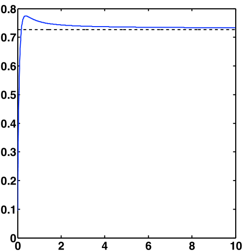
Refer to caption
Figure 7: Convergence of u(T,y)T𝑢𝑇𝑦𝑇\frac{u(T,y)}{T} towards a constant value λHJsubscript𝜆𝐻𝐽\lambda_{HJ}. We have plotted a specific value at an arbitrary point y0𝒮subscript𝑦0𝒮y_{0}\in\mathcal{S}. We observe that the limiting value λHJsubscript𝜆𝐻𝐽\lambda_{HJ} is close to the maximal Perron eigenvalue λP0.7273subscript𝜆𝑃0.7273\lambda_{P}\approx 0.7273 (dashed line, see also Figure 1). The discrepancy between the limiting value and λPsubscript𝜆𝑃\lambda_{P} (dashed line) falls below the numerical error due to the scheme, which is of order one.
Refer to caption

(a) Refer to caption(b)

Refer to caption

(c) Refer to caption(d)

Figure 8: (a) The function u(T,y)𝑢𝑇𝑦u(T,y) presumably converges to an eigenvector u¯¯𝑢\overline{u} as T+𝑇T\to+\infty, modulo a constant of order λHJTsubscript𝜆𝐻𝐽𝑇\lambda_{HJ}T. (b) Level sets of the function u¯¯𝑢\overline{u} and the separation line where the optimal control switches from a𝑎a to A𝐴A. (c) and (d) Derivatives of the function u¯¯𝑢\overline{u} with respect to the first and the second variable.
Refer to caption

(a) Refer to caption(b)

Figure 9: (a) An optimal trajectory starting from the upper corner of the simplex. It presumably converges towards the optimal eigenvector eαsubscript𝑒superscript𝛼e_{\alpha^{*}}. The optimal trajectory appears to be glued to the separation line. (b) The corresponding optimal control α(t)𝛼𝑡\alpha(t) is plotted in blue. It oscillates rapidly between the two extremal values a=1,A=6formulae-sequence𝑎1𝐴6a=1,A=6. It converges weakly to α=3.35superscript𝛼3.35\alpha^{*}=3.35 as the time step ΔtΔ𝑡\Delta t goes to zero (here, Δt=103Δ𝑡superscript103\Delta t=10^{-3}), as can be observed when averaging the function α(t)𝛼𝑡\alpha(t) (in red: local average of α(t)𝛼𝑡\alpha(t) with a span of 100Δt100Δ𝑡100\Delta t).
Growth in the first compartment τ1=0.5subscript𝜏10.5\tau_{1}=0.5
Growth in the second compartment τ2=5subscript𝜏25\tau_{2}=5
fragmentation in the second compartment β2=1subscript𝛽21\beta_{2}=1
fragmentation in the third compartment β3=2subscript𝛽32\beta_{3}=2
minimal rate of sonication a=1𝑎1a=1
maximal rate of sonication A=6𝐴6A=6
optimal rate of sonication (constant control) α=3.35superscript𝛼3.35\alpha^{*}=3.35
space step in the simplex Δy=102Δ𝑦superscript102\Delta y=10^{-2}
time step Δt=103Δ𝑡superscript103\Delta t=10^{-3}
final time of computation T=10𝑇10T=10
Table 1: Set of parameters for illustrations and numerical simulations.

All the numerical simulations shown in Section 3 have been performed for the running example (1.4) with parameters listed in Table 1. We have solved numerically the Hamilton-Jacobi-Bellman equation (3.1) using a classical upwind scheme for the discretization of the Hamiltonian (3.2). We observe that the quantity u(T,y)T𝑢𝑇𝑦𝑇\frac{u(T,y)}{T} converges to a constant value λHJsubscript𝜆𝐻𝐽\lambda_{HJ} which is close to the Perron eigenvalue λP(α)subscript𝜆𝑃superscript𝛼\lambda_{P}(\alpha^{*}). The discrepancy in the limit falls within the range of error due to the numerical scheme. Furthermore, we observe that the function u(T,y)λHJT𝑢𝑇𝑦subscript𝜆𝐻𝐽𝑇u(T,y)-\lambda_{HJ}T presumably converges to an eigenvector u¯¯𝑢\overline{u} (Figure 8).

We notice that the numerical scheme selects either a𝑎a or A𝐴A at each step because of the very definition of the hamiltonian (3.2). It is quite instructive to plot the line where the control switches from a𝑎a to A𝐴A, namely where Fy,Dyu¯=0𝐹𝑦subscript𝐷𝑦¯𝑢0\left\langle Fy,D_{y}\overline{u}\right\rangle=0. We call it the separation line (Figure 8b). Apparently the optimal eigenvector eαsubscript𝑒superscript𝛼e_{\alpha^{*}} belongs to this line. We observe numerically that the optimal trajectories are glued to this separation line (Figure 9a). We observe fast oscillations between the extremal values a𝑎a and A𝐴A at the scale of the time step (see Figure 9b). The values a𝑎a and A𝐴A are chosen in such a way that local averaging over several time steps yields a constant control αsuperscript𝛼\alpha^{*}. We conjecture that the control α(t)𝛼𝑡\alpha(t) obtained through a bang-bang procedure (thus taking extremal values a𝑎a and A𝐴A) converges weakly to the constant control αsuperscript𝛼\alpha^{*} in infinite horizon.

We now list perspectives for future attention, by discussing the assumptions made in the present work. The first question concerns the higher-dimensional case. Here the two dimensional structure of the simplex plays a crucial role. For instance, it is not even clear how to define properly the ergodic set in higher dimension of space. A natural extension would be to study the case where the control α(t)𝛼𝑡\alpha(t) has N1𝑁1N-1 degree of freedom, where N𝑁N is the dimension of the simplex (the original problem (1.1) being of dimension N+1𝑁1N+1). Next we discuss ways to remove the hypotheses (H1-2-3-4-5), separately.
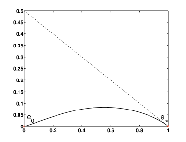
Refer to caption

(a)  Refer to caption(b)

Refer to caption

(c)   Refer to caption(d)

Figure 10: Discussion of Hypotheses (H1)-(H3). We have plotted the zero level set of the cubic function Φ0={y𝒮:φ(y)=0}subscriptΦ0conditional-set𝑦𝒮𝜑𝑦0\Phi_{0}=\{y\in\mathcal{S}\;:\;\varphi(y)=0\} together with the extremal eigenvectors e0subscript𝑒0e_{0} and esubscript𝑒e_{\infty} in four cases: (a) G𝐺G and F𝐹F are both reducible (i.e. the running example (1.4)), (b) G𝐺G is irreducible and F𝐹F is reducible, (c) G𝐺G is reducible and F𝐹F is irreducible, (d) G𝐺G and F𝐹F are both irreducible. We have modified F𝐹F such that we still have mTF=0superscript𝑚𝑇𝐹0m^{T}F=0.
Refer to caption

(a)  Refer to caption(b)

Refer to caption

(c) Refer to caption(d)

Figure 11: Discussion of Hypothesis (H2). Here, τ1=τ2=0.5subscript𝜏1subscript𝜏20.5\tau_{1}=\tau_{2}=0.5, a=1𝑎1a=1 and A=6𝐴6A=6. The function λ(α)𝜆𝛼\lambda(\alpha) is increasing (a). The optimal control is α(t)=A𝛼𝑡𝐴\alpha(t)=A. Consequently λ=λP(A)superscript𝜆subscript𝜆𝑃𝐴\lambda^{*}=\lambda_{P}(A). The eigenvector is also known: u¯(y)=logϕA,y¯𝑢𝑦subscriptitalic-ϕ𝐴𝑦\overline{u}(y)=\log\left\langle\phi_{A},y\right\rangle. This claim is confirmed by numerical simulations: the level sets of u(T,y)𝑢𝑇𝑦u(T,y) are straight lines (b). The slope of the lines is in accordance with ϕAsubscriptitalic-ϕ𝐴\phi_{A} (the thick line is directed by mϕAT𝒮𝑚subscriptitalic-ϕ𝐴𝑇𝒮m\wedge\phi_{A}\in T\mathcal{S}). The gradient of the function exp(u(T,y)u(T,y0))𝑢𝑇𝑦𝑢𝑇subscript𝑦0\exp(u(T,y)-u(T,y_{0})) is almost constant: observe the small amplitude in (c) and (d).
Refer to caption
Figure 12: Construction of the subset 𝒮superscript𝒮\mathcal{S}^{\prime}: the segment [y,e]𝑦subscript𝑒[y,e_{\infty}] crosses the line Φ0subscriptΦ0\Phi_{0} on eβsubscript𝑒𝛽e_{\beta} with βA𝛽superscript𝐴\beta\leq A^{\prime}
Refer to caption

(a)  Refer to caption(b)

Refer to caption

(c)  Refer to caption(d)

Figure 13: Discussion of Hypothesis (H2). Here, τ1=0.5subscript𝜏10.5\tau_{1}=0.5, τ2=5subscript𝜏25\tau_{2}=5, a=0.5𝑎0.5a=0.5 and A=2𝐴2A=2. The function λ(α)𝜆𝛼\lambda(\alpha) is increasing up to α=3.35superscript𝛼3.35\alpha^{*}=3.35, then decreasing (a). The eigenvector is known on a subpart 𝒮𝒮superscript𝒮𝒮\mathcal{S}^{\prime}\subset\mathcal{S}, where 𝒮superscript𝒮\mathcal{S}^{\prime} is defined in the text: y𝒮u¯(y)=logϕA,yfor-all𝑦superscript𝒮¯𝑢𝑦subscriptitalic-ϕ𝐴𝑦\forall y\in\mathcal{S}^{\prime}\;\overline{u}(y)=\log\left\langle\phi_{A},y\right\rangle. This claim is confirmed by numerical simulations: the level sets of u(T,y)𝑢𝑇𝑦u(T,y) are straight lines on 𝒮superscript𝒮\mathcal{S}^{\prime} (b). The slope of the lines is in accordance with ϕAsubscriptitalic-ϕ𝐴\phi_{A} (the thick line is directed by mϕAT𝒮𝑚subscriptitalic-ϕ𝐴𝑇𝒮m\wedge\phi_{A}\in T\mathcal{S}). The gradient of the function exp(u(T,y)u(T,y0))𝑢𝑇𝑦𝑢𝑇subscript𝑦0\exp(u(T,y)-u(T,y_{0})) is plotted in (c) and (d).
(H1)-(H3)

In the case where G𝐺G or F𝐹F is irreducible, the limiting eigenvectors do not lie on the boundary of the simplex. Therefore the line of Perron eigenvectors {eβ: 0β}conditional-setsubscript𝑒𝛽 0𝛽\{e_{\beta}:\;0\leq\beta\leq\infty\} does not divide the simplex into two parts. However the line Φ0={y𝒮:φ(y)=0}subscriptΦ0conditional-set𝑦𝒮𝜑𝑦0\Phi_{0}=\{y\in\mathcal{S}\;:\;\varphi(y)=0\} does so. It is the zero level set of a cubic function. We have plotted in Figure 10 several examples, for the cases where G𝐺G or F𝐹F, or both, are irreducible.

(H2)

When the Perron eigenvalue λP(α)subscript𝜆𝑃𝛼\lambda_{P}(\alpha) is nondecreasing with respect to α𝛼\alpha and bounded (cf. Proposition 2.1 for the running example), we have maxα[a,A]λP(α)=λP(A)subscript𝛼𝑎𝐴subscript𝜆𝑃𝛼subscript𝜆𝑃𝐴\max_{\alpha\in[a,A]}\lambda_{P}(\alpha)=\lambda_{P}(A). Our strategy of proof does not contain this particular example (see Step 6). Nevertheless, under an additional assumption (see below) we exhibit a particular solution to (3.1) with a different initial condition, namely

u(t,y)=λP(A)t+logϕA,y.𝑢𝑡𝑦subscript𝜆𝑃𝐴𝑡subscriptitalic-ϕ𝐴𝑦u(t,y)=\lambda_{P}(A)t+\log\left\langle\phi_{A},y\right\rangle\,. (4.1)

Interestingly this coincides with the expansion of rα(T,x)subscript𝑟𝛼𝑇𝑥r_{\alpha}(T,x) in the case of constant control α=A𝛼𝐴\alpha=A (2.1). Moreover the function u¯(y)=logϕA,y¯𝑢𝑦subscriptitalic-ϕ𝐴𝑦\overline{u}(y)=\log\left\langle\phi_{A},y\right\rangle is a good candidate for being the Hamilton-Jacobi eigenvector. It is a viscosity solution of the ergodic stationary equation,

λP(A)+H(y,Dyu¯(y))=0.subscript𝜆𝑃𝐴𝐻𝑦subscript𝐷𝑦¯𝑢𝑦0-\lambda_{P}(A)+H(y,D_{y}\overline{u}(y))=0\,.

In Figure 11 we show numerical simulations which confirm that this particular solution describes well the asymptotic behaviour of solutions to (3.1).
To assert that u(t,y)𝑢𝑡𝑦u(t,y) given by (4.1) is a particular solution of (3.1) we check that the optimality condition is verified for α=A𝛼𝐴\alpha=A,

maxα[a,A]b(y,α),Dyusubscript𝛼𝑎𝐴𝑏𝑦𝛼subscript𝐷𝑦𝑢\displaystyle\max_{\alpha\in[a,A]}\left\langle b(y,\alpha),D_{y}u\right\rangle =maxα[a,A]{(G+αF)y,ϕAy,ϕAm,Gy}absentsubscript𝛼𝑎𝐴𝐺𝛼𝐹𝑦subscriptitalic-ϕ𝐴𝑦subscriptitalic-ϕ𝐴𝑚𝐺𝑦\displaystyle=\max_{\alpha\in[a,A]}\left\{\dfrac{\left\langle(G+\alpha F)y,\phi_{A}\right\rangle}{\left\langle y,\phi_{A}\right\rangle}-\left\langle m,Gy\right\rangle\right\}
=maxα[a,A]{λP(A)+(αA)Fy,ϕAy,ϕA}absentsubscript𝛼𝑎𝐴subscript𝜆𝑃𝐴𝛼𝐴𝐹𝑦subscriptitalic-ϕ𝐴𝑦subscriptitalic-ϕ𝐴\displaystyle=\max_{\alpha\in[a,A]}\left\{\lambda_{P}(A)+(\alpha-A)\frac{\left\langle Fy,\phi_{A}\right\rangle}{\left\langle y,\phi_{A}\right\rangle}\right\}
=λP(A).absentsubscript𝜆𝑃𝐴\displaystyle=\lambda_{P}(A)\,.

The optimality condition is satisfied if Fy,ϕA0𝐹𝑦subscriptitalic-ϕ𝐴0\left\langle Fy,\phi_{A}\right\rangle\geq 0 for all y𝒮𝑦𝒮y\in\mathcal{S}. This condition is guaranteed under the two following conditions: (i) αλP(α)maps-to𝛼subscript𝜆𝑃𝛼\alpha\mapsto\lambda_{P}(\alpha) is nondecreasing, and (ii) for all y𝒮𝑦𝒮y\in\mathcal{S} the segment [y,e]𝑦subscript𝑒[y,e_{\infty}] crosses the line of eigenvectors Φ0subscriptΦ0\Phi_{0}, where esubscript𝑒e_{\infty} is a corner of the simplex (Figure 12). The second condition is satisfied for the running example since in this case e0=(0 0 1/3)Tsubscript𝑒0superscript0013𝑇e_{0}=(0\ 0\ 1/3)^{T} and e=(1 0 0)Tsubscript𝑒superscript100𝑇e_{\infty}=(1\ 0\ 0)^{T} are corners of the simplex 𝒮𝒮\mathcal{S} and the tangent to Φ0subscriptΦ0\Phi_{0} at the point esubscript𝑒e_{\infty}, given by the vector Gem,Gee=τ1(2 1 0)T,𝐺subscript𝑒𝑚𝐺subscript𝑒subscript𝑒subscript𝜏1superscript210𝑇Ge_{\infty}-\left\langle m,Ge_{\infty}\right\rangle e_{\infty}=\tau_{1}(-2\ 1\ 0)^{T}, coincides with the edge of the simplex which does not contain e0subscript𝑒0e_{0}. We introduce the intersection point eβΦ0subscript𝑒𝛽subscriptΦ0e_{\beta}\in\Phi_{0}. We decompose y=cβeβ+ce𝑦subscript𝑐𝛽subscript𝑒𝛽subscript𝑐subscript𝑒y=c_{\beta}e_{\beta}+c_{\infty}e_{\infty}, with cβ0subscript𝑐𝛽0c_{\beta}\geq 0 (and csubscript𝑐c_{\infty}\in\mathbb{R}). We have on the one hand,

λP(A)ϕA,eβ=ϕA(G+AF)eβ=λP(β)ϕA,eβ+(Aβ)ϕA,Feβ.subscript𝜆𝑃𝐴subscriptitalic-ϕ𝐴subscript𝑒𝛽subscriptitalic-ϕ𝐴𝐺𝐴𝐹subscript𝑒𝛽subscript𝜆𝑃𝛽subscriptitalic-ϕ𝐴subscript𝑒𝛽𝐴𝛽subscriptitalic-ϕ𝐴𝐹subscript𝑒𝛽\lambda_{P}(A)\left\langle\phi_{A},e_{\beta}\right\rangle=\phi_{A}(G+AF)e_{\beta}=\lambda_{P}(\beta)\left\langle\phi_{A},e_{\beta}\right\rangle+(A-\beta)\left\langle\phi_{A},Fe_{\beta}\right\rangle\,.

On the other hand we get since Fe=0𝐹subscript𝑒0Fe_{\infty}=0,

Fy,ϕA𝐹𝑦subscriptitalic-ϕ𝐴\displaystyle\left\langle Fy,\phi_{A}\right\rangle =cβFeβ,ϕA+cFe,ϕAabsentsubscript𝑐𝛽𝐹subscript𝑒𝛽subscriptitalic-ϕ𝐴subscript𝑐𝐹subscript𝑒subscriptitalic-ϕ𝐴\displaystyle=c_{\beta}\left\langle Fe_{\beta},\phi_{A}\right\rangle+c_{\infty}\left\langle Fe_{\infty},\phi_{A}\right\rangle
=cβλP(A)λP(β)AβϕA,eβ0.absentsubscript𝑐𝛽subscript𝜆𝑃𝐴subscript𝜆𝑃𝛽𝐴𝛽subscriptitalic-ϕ𝐴subscript𝑒𝛽0\displaystyle=c_{\beta}\dfrac{\lambda_{P}(A)-\lambda_{P}(\beta)}{A-\beta}\left\langle\phi_{A},e_{\beta}\right\rangle\geq 0\,.

The same result holds true in the case where λP(α)subscript𝜆𝑃𝛼\lambda_{P}(\alpha) is increasing up to A𝐴A, and satisfies λP(β)λP(A)subscript𝜆𝑃𝛽subscript𝜆𝑃𝐴\lambda_{P}(\beta)\geq\lambda_{P}(A) for all β>A𝛽𝐴\beta>A.
Last but not least, in the case where λP(α)subscript𝜆𝑃𝛼\lambda_{P}(\alpha) is increasing up to A𝐴A, and there exists A>Asuperscript𝐴𝐴A^{\prime}>A such that λP(A)=λP(A)subscript𝜆𝑃superscript𝐴subscript𝜆𝑃𝐴\lambda_{P}(A^{\prime})=\lambda_{P}(A) the situation is quite different. We choose the smallest possible A>Asuperscript𝐴𝐴A^{\prime}>A. The function defined by (4.1) is a particular solution only on the subset of the simplex 𝒮superscript𝒮\mathcal{S}^{\prime} defined by the following rule: y𝒮𝑦superscript𝒮y\in\mathcal{S}^{\prime} if the segment [y,e]𝑦subscript𝑒[y,e_{\infty}] crosses the line Φ0subscriptΦ0\Phi_{0} on eβsubscript𝑒𝛽e_{\beta} with βA𝛽superscript𝐴\beta\leq A^{\prime} (Figures 12 and 13).

(H4)

When the quantity (3.5) does not have a constant sign, we cannot rule out the situation where the trajectories cross the line of eigenvectors Φ0subscriptΦ0\Phi_{0} anywhere. This causes problems on the proper definition of the ergodic set 𝒵0subscript𝒵0\mathcal{Z}_{0} (see also discussion of how to remove (H5) below). This also causes problems on the monotonicity formulas (3.13)-(3.14). However we believe this is just a technical assumption. When the quantity deβdβ,ΘFeβ|ΘFeβ|𝑑subscript𝑒𝛽𝑑𝛽Θ𝐹subscript𝑒𝛽Θ𝐹subscript𝑒𝛽\left\langle\frac{de_{\beta}}{d\beta},\frac{\Theta Fe_{\beta}}{|\Theta Fe_{\beta}|}\right\rangle changes sign then we may switch the parametrization from A+δ𝐴𝛿A+\delta to aδ𝑎𝛿a-\delta, or vice-versa, to preserve the monotonicity of β(t)𝛽𝑡\beta(t).

(H5)

This Hypothesis is essential to build properly the ergodic set 𝒵0subscript𝒵0\mathcal{Z}_{0} in our way. In fact it guarantees that the trajectories which define the boundary 𝒵0subscript𝒵0\partial\mathcal{Z}_{0} lie on the two opposite sides of Φ0subscriptΦ0\Phi_{0}. This rules out a possible spiraling phenomenon. It could be possible to define the ergodic set 𝒵0subscript𝒵0\mathcal{Z}_{0} in another way but this would lead to increasing complexity of the preceding steps.
We propose the following construction: starting from easubscript𝑒𝑎e_{a}, the trajectory γAasuperscriptsubscript𝛾𝐴𝑎\gamma_{A}^{a} crosses Φ0subscriptΦ0\Phi_{0} on eβ1subscript𝑒subscript𝛽1e_{\beta_{1}} with β1Asubscript𝛽1𝐴\beta_{1}\geq A due to Assumption (H4). If β1>Asubscript𝛽1𝐴\beta_{1}>A we need to switch the control after crossing Φ0subscriptΦ0\Phi_{0} to preserve the monotonicity formula (Lemma 3.9). The trajectory starting from eβ1subscript𝑒subscript𝛽1e_{\beta_{1}} with constant control a𝑎a, γaβ1superscriptsubscript𝛾𝑎subscript𝛽1\gamma_{a}^{\beta_{1}} reaches Φ0subscriptΦ0\Phi_{0} on eβ2subscript𝑒subscript𝛽2e_{\beta_{2}} with β2asubscript𝛽2𝑎\beta_{2}\leq a due to Assumption (H4). If β2=asubscript𝛽2𝑎\beta_{2}=a we are done: the two portions of trajectories γAasuperscriptsubscript𝛾𝐴𝑎\gamma_{A}^{a} and γaβ1superscriptsubscript𝛾𝑎subscript𝛽1\gamma_{a}^{\beta_{1}} enclose a stable set 𝒵0subscript𝒵0\mathcal{Z}_{0} which is a good candidate to being the ergodic set.
If β2<asubscript𝛽2𝑎\beta_{2}<a however we switch again: the trajectory starting from eβ2subscript𝑒subscript𝛽2e_{\beta_{2}} with constant control A𝐴A, γAβ2superscriptsubscript𝛾𝐴subscript𝛽2\gamma_{A}^{\beta_{2}} reaches Φ0subscriptΦ0\Phi_{0} on eβ3subscript𝑒subscript𝛽3e_{\beta_{3}} with β3>β1subscript𝛽3subscript𝛽1\beta_{3}>\beta_{1} (because trajectories cannot cross). We define iteratively two monotonic sequences β2isubscript𝛽2𝑖\beta_{2i} and β2i+1subscript𝛽2𝑖1\beta_{2i+1} (resp. decreasing and increasing) such that β2i<asubscript𝛽2𝑖𝑎\beta_{2i}<a and β2(i+1)>Asubscript𝛽2𝑖1𝐴\beta_{2(i+1)}>A. The two limits β¯<β2i<a<A<β2(i+1)<β¯¯𝛽subscript𝛽2𝑖𝑎𝐴subscript𝛽2𝑖1¯𝛽\underline{\beta}<\beta_{2i}<a<A<\beta_{2(i+1)}<\overline{\beta} define the boundary of a stable and controllable set 𝒵0subscript𝒵0\mathcal{Z}_{0} through the following periodic cycle: starting from eβ¯subscript𝑒¯𝛽e_{\underline{\beta}} the trajectory with constant control A𝐴A reaches eβ¯subscript𝑒¯𝛽e_{\overline{\beta}} in finite time, and the trajectory starting from eβ¯subscript𝑒¯𝛽e_{\overline{\beta}} with constant control a𝑎a reaches eβ¯subscript𝑒¯𝛽e_{\underline{\beta}} in finite time.
We cannot rule out the existence of several such periodic cycles (with control a𝑎a on Φ+superscriptΦ\Phi^{+} and control A𝐴A on ΦsuperscriptΦ\Phi^{-}). In this case the set 𝒵0subscript𝒵0\mathcal{Z}_{0} constructed above is certainly not attractive, because 𝒵0subscript𝒵0\mathcal{Z}_{0} does not contain any other cycle than its boundary.


Acknowledgements. The authors have benefited from stimulating discussions with Stéphane Gaubert, Thomas Lepoutre and Maxime Zavidovique. They warmly thank Marie Doumic for having coordinated the ANR Grant ANR-09-BLAN-0218 TOPPAZ, in which both authors were involved. The early motivation for this work comes from illuminating discussions with Natacha Lennuzza and Franck Mouthon, from whom the authors have learned everything they know about Prion proliferation and PMCA.


Appendix

Appendix A Diagonalisation of G+αF𝐺𝛼𝐹G+\alpha F

In the case of the running example, we give a condition for which the matrix G+αF𝐺𝛼𝐹G+\alpha F is diagonalisable (in \mathbb{R}).

Proposition A.1.

Consider the matrices G𝐺G and F𝐹F defined in (1.4), with the condition τ2>2τ1.subscript𝜏22subscript𝜏1\tau_{2}>2\tau_{1}. Then the matrix G+αF𝐺𝛼𝐹G+\alpha F is diagonalisable in {\mathbb{R}} for any α>0.𝛼0\alpha>0. Furthermore, the three real eigenvalues satisfy

λ1>0>λ2>λ3.superscriptsubscript𝜆10subscript𝜆2subscript𝜆3\lambda_{1}^{*}>0>\lambda_{2}>\lambda_{3}.
Proof.

We compute the value of the characteristic polynomial of G+αF𝐺𝛼𝐹G+\alpha F at x=0𝑥0x=0

P(0)=ατ1τ2β3α2τ1β2β3<0𝑃0𝛼subscript𝜏1subscript𝜏2subscript𝛽3superscript𝛼2subscript𝜏1subscript𝛽2subscript𝛽30P(0)=-\alpha\tau_{1}\tau_{2}\beta_{3}-\alpha^{2}\tau_{1}\beta_{2}\beta_{3}<0

as for two well chosen negative values

P(αβ3)=ατ2β3(αβ32τ1)𝑃𝛼subscript𝛽3𝛼subscript𝜏2subscript𝛽3𝛼subscript𝛽32subscript𝜏1P(-\alpha\beta_{3})=\alpha\tau_{2}\beta_{3}(\alpha\beta_{3}-2\tau_{1})

and

P(τ2)=αβ2(τ22+τ1τ2)+αβ3(τ222τ1τ2)α2(τ1+τ2)β2β3.𝑃subscript𝜏2𝛼subscript𝛽2superscriptsubscript𝜏22subscript𝜏1subscript𝜏2𝛼subscript𝛽3superscriptsubscript𝜏222subscript𝜏1subscript𝜏2superscript𝛼2subscript𝜏1subscript𝜏2subscript𝛽2subscript𝛽3P(-\tau_{2})=\alpha\beta_{2}(\tau_{2}^{2}+\tau_{1}\tau_{2})+\alpha\beta_{3}(\tau_{2}^{2}-2\tau_{1}\tau_{2})-\alpha^{2}(\tau_{1}+\tau_{2})\beta_{2}\beta_{3}.

We notice that

P(αβ3)>0α>2τ1β3formulae-sequence𝑃𝛼subscript𝛽30𝛼2subscript𝜏1subscript𝛽3P(-\alpha\beta_{3})>0\quad\Leftrightarrow\quad\alpha>\frac{2\tau_{1}}{\beta_{3}}

and

P(τ2)>0α<τ2β3+τ2τ1τ2τ22τ1β2.formulae-sequence𝑃subscript𝜏20𝛼subscript𝜏2subscript𝛽3subscript𝜏2subscript𝜏1subscript𝜏2subscript𝜏22𝜏1subscript𝛽2P(-\tau_{2})>0\quad\Leftrightarrow\quad\alpha<\frac{\tau_{2}}{\beta_{3}}+\frac{\tau_{2}}{\tau_{1}\tau_{2}}\frac{\tau_{2}-2\tau 1}{\beta_{2}}.

Because τ2>2τ1,subscript𝜏22subscript𝜏1\tau_{2}>2\tau_{1}, we have

τ2β3+τ2τ1τ2τ22τ1β2>τ2β3>2τ1β3subscript𝜏2subscript𝛽3subscript𝜏2subscript𝜏1subscript𝜏2subscript𝜏22𝜏1subscript𝛽2subscript𝜏2subscript𝛽32subscript𝜏1subscript𝛽3\frac{\tau_{2}}{\beta_{3}}+\frac{\tau_{2}}{\tau_{1}\tau_{2}}\frac{\tau_{2}-2\tau 1}{\beta_{2}}>\frac{\tau_{2}}{\beta_{3}}>\frac{2\tau_{1}}{\beta_{3}}

so if P(αβ3)0,𝑃𝛼subscript𝛽30P(-\alpha\beta_{3})\leq 0, then P(τ2)>0.𝑃subscript𝜏20P(-\tau_{2})>0. Finally P𝑃P is a third order polynomial which satisfies the following properties: (i) it tends to -\infty at -\infty; (ii) it takes positive values for negative x𝑥x; (iii) it is negative at x=0𝑥0x=0; (iv) it tends to ++\infty at ++\infty. Thus P𝑃P has 3 real roots and it proves the proposition. ∎

Appendix B Criterion for Assumption (H4)
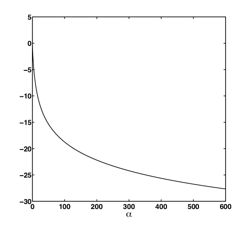
Refer to caption
Figure 14: Numerical check of the Assumption (H4) for the running example, by using the formula in Proposition B.1. Plot of the quantity deαdα,ΘFeα𝑑subscript𝑒𝛼𝑑𝛼Θ𝐹subscript𝑒𝛼-\left\langle\frac{de_{\alpha}}{d\alpha},\Theta Fe_{\alpha}\right\rangle as a function of α𝛼\alpha in log-scale.
Proposition B.1.

Denoting (e1,e2,e3)subscript𝑒1subscript𝑒2subscript𝑒3(e_{1},e_{2},e_{3}) a basis of eigenvectors for G+αF,𝐺𝛼𝐹G+\alpha F, so that e1=eα,subscript𝑒1subscript𝑒𝛼e_{1}=e_{\alpha}, and (ϕ1,ϕ2,ϕ3)subscriptitalic-ϕ1subscriptitalic-ϕ2subscriptitalic-ϕ3(\phi_{1},\phi_{2},\phi_{3}) a basis of dual eigenvectors, we have the formula

deαdα,ΘFeα=λ2λ3(λ1λ2)(λ1λ3)(ϕ2Fe1)(ϕ3Fe1)e2e1,Θ(e3e1).𝑑subscript𝑒𝛼𝑑𝛼Θ𝐹subscript𝑒𝛼subscript𝜆2subscript𝜆3subscript𝜆1subscript𝜆2subscript𝜆1subscript𝜆3subscriptitalic-ϕ2𝐹subscript𝑒1subscriptitalic-ϕ3𝐹subscript𝑒1subscript𝑒2subscript𝑒1Θsubscript𝑒3subscript𝑒1\left\langle\frac{de_{\alpha}}{d\alpha},\Theta Fe_{\alpha}\right\rangle=\frac{\lambda_{2}-\lambda_{3}}{(\lambda_{1}-\lambda_{2})(\lambda_{1}-\lambda_{3})}(\phi_{2}Fe_{1})(\phi_{3}Fe_{1})\left\langle e_{2}-e_{1},\Theta(e_{3}-e_{1})\right\rangle.
Proof.

Decompose deαdα𝑑subscript𝑒𝛼𝑑𝛼\frac{de_{\alpha}}{d\alpha} and Feα𝐹subscript𝑒𝛼Fe_{\alpha} along the basis (e1,e2,e3)::subscript𝑒1subscript𝑒2subscript𝑒3absent(e_{1},e_{2},e_{3}):

deαdα=a1e1+a2e2+a3e3,Feα=b1e1+b2e2+b3e3.formulae-sequence𝑑subscript𝑒𝛼𝑑𝛼subscript𝑎1subscript𝑒1subscript𝑎2subscript𝑒2subscript𝑎3subscript𝑒3𝐹subscript𝑒𝛼subscript𝑏1subscript𝑒1subscript𝑏2subscript𝑒2subscript𝑏3subscript𝑒3\frac{de_{\alpha}}{d\alpha}=a_{1}e_{1}+a_{2}e_{2}+a_{3}e_{3},\qquad Fe_{\alpha}=b_{1}e_{1}+b_{2}e_{2}+b_{3}e_{3}.

For all α𝛼\alpha we have m,eα=1𝑚subscript𝑒𝛼1\left\langle m,e_{\alpha}\right\rangle=1 because eα𝒮,subscript𝑒𝛼𝒮e_{\alpha}\in\mathcal{S}, so m,deαdα=0.𝑚𝑑subscript𝑒𝛼𝑑𝛼0\left\langle m,\frac{de_{\alpha}}{d\alpha}\right\rangle=0. Because mTF=0,superscript𝑚𝑇𝐹0m^{T}F=0, we also have m,Feα=0.𝑚𝐹subscript𝑒𝛼0\left\langle m,Fe_{\alpha}\right\rangle=0. It leads to the relations

a1+a2+a3=b1+b2+b3=0.subscript𝑎1subscript𝑎2subscript𝑎3subscript𝑏1subscript𝑏2subscript𝑏30a_{1}+a_{2}+a_{3}=b_{1}+b_{2}+b_{3}=0.

As a consequence we have

deαdα,ΘFeα𝑑subscript𝑒𝛼𝑑𝛼Θ𝐹subscript𝑒𝛼\displaystyle\left\langle\frac{de_{\alpha}}{d\alpha},\Theta Fe_{\alpha}\right\rangle =a2(e2e1)+a3(e3e1),b2Θ(e2e1)+b3Θ(e3e1)absentsubscript𝑎2subscript𝑒2subscript𝑒1subscript𝑎3subscript𝑒3subscript𝑒1subscript𝑏2Θsubscript𝑒2subscript𝑒1subscript𝑏3Θsubscript𝑒3subscript𝑒1\displaystyle=\left\langle a_{2}(e_{2}-e_{1})+a_{3}(e_{3}-e_{1}),b_{2}\Theta(e_{2}-e_{1})+b_{3}\Theta(e_{3}-e_{1})\right\rangle
=a2b3(e2e1),Θ(e3e1)+a3b2(e3e1),Θ(e2e1).absentsubscript𝑎2subscript𝑏3subscript𝑒2subscript𝑒1Θsubscript𝑒3subscript𝑒1subscript𝑎3subscript𝑏2subscript𝑒3subscript𝑒1Θsubscript𝑒2subscript𝑒1\displaystyle=a_{2}b_{3}\left\langle(e_{2}-e_{1}),\Theta(e_{3}-e_{1})\right\rangle+a_{3}b_{2}\left\langle(e_{3}-e_{1}),\Theta(e_{2}-e_{1})\right\rangle.

Now we look for a relation between aisubscript𝑎𝑖a_{i} and bisubscript𝑏𝑖b_{i} and we start from

(G+αF)eα=λ(α)eα𝐺𝛼𝐹subscript𝑒𝛼𝜆𝛼subscript𝑒𝛼(G+\alpha F)e_{\alpha}=\lambda(\alpha)e_{\alpha}

which gives after differentiation with respect to α𝛼\alpha

(G+αF)deαdα+Feα=λαdeαdα+λ(α)eα.𝐺𝛼𝐹𝑑subscript𝑒𝛼𝑑𝛼𝐹subscript𝑒𝛼subscript𝜆𝛼𝑑subscript𝑒𝛼𝑑𝛼superscript𝜆𝛼subscript𝑒𝛼(G+\alpha F)\frac{de_{\alpha}}{d\alpha}+Fe_{\alpha}=\lambda_{\alpha}\frac{de_{\alpha}}{d\alpha}+\lambda^{\prime}(\alpha)e_{\alpha}.

Testing against ϕisubscriptitalic-ϕ𝑖\phi_{i} with i{2,3},𝑖23i\in\{2,3\}, we obtain

λiϕideαdα+ϕiFe1=λ1ϕideαdα.subscript𝜆𝑖subscriptitalic-ϕ𝑖𝑑subscript𝑒𝛼𝑑𝛼subscriptitalic-ϕ𝑖𝐹subscript𝑒1subscript𝜆1subscriptitalic-ϕ𝑖𝑑subscript𝑒𝛼𝑑𝛼\lambda_{i}\phi_{i}\frac{de_{\alpha}}{d\alpha}+\phi_{i}Fe_{1}=\lambda_{1}\phi_{i}\frac{de_{\alpha}}{d\alpha}.

Finally we find

bi=ϕiFe1=(λ1λi)ϕideαdα=(λ1λi)aisubscript𝑏𝑖subscriptitalic-ϕ𝑖𝐹subscript𝑒1subscript𝜆1subscript𝜆𝑖subscriptitalic-ϕ𝑖𝑑subscript𝑒𝛼𝑑𝛼subscript𝜆1subscript𝜆𝑖subscript𝑎𝑖b_{i}=\phi_{i}Fe_{1}=(\lambda_{1}-\lambda_{i})\phi_{i}\frac{de_{\alpha}}{d\alpha}=(\lambda_{1}-\lambda_{i})a_{i}

and the result of the proposition follows. ∎

References

  • [1] O. Alvarez and M. Bardi. Ergodicity, stabilization, and singular perturbations for Bellman-Isaacs equations. Mem. Amer. Math. Soc., 204(960):vi+77, 2010.
  • [2] M. Arisawa. Ergodic problem for the Hamilton-Jacobi-Bellman equation. I. Existence of the ergodic attractor. Annales de l’Institut Henri Poincaré (C) Non Linear Analysis, 14(4):415–438, 1997.
  • [3] M. Arisawa. Ergodic problem for the Hamilton-Jacobi-Bellman equation. II. Annales de l’Institut Henri Poincaré (C) Non Linear Analysis, 15(1):1–24, 1998.
  • [4] M. Arisawa and P.-L. Lions. On ergodic stochastic control. Communications in Partial Differential Equations, 23(11-12):333–358, 1998.
  • [5] M. Bardi and I. Capuzzo-Dolcetta. Optimal control and viscosity solutions of Hamilton-Jacobi-Bellman equations. Systems & Control: Foundations & Applications. Birkhäuser Boston Inc., Boston, MA, 1997. With appendices by Maurizio Falcone and Pierpaolo Soravia.
  • [6] G. Barles. Some homogenization results for non-coercive Hamilton-Jacobi equations. Calc. Var. Partial Differential Equations, 30(4):449–466, 2007.
  • [7] G. Barles, L. C. Evans, and P. E. Souganidis. Wavefront propagation for reaction-diffusion systems of PDE. Duke Math. J., 61(3):835–858, 1990.
  • [8] G. Barles and J.-M. Roquejoffre. Ergodic type problems and large time behaviour of unbounded solutions of Hamilton-Jacobi equations. Comm. Partial Differential Equations, 31(7-9):1209–1225, 2006.
  • [9] G. Barles and P. E. Souganidis. On the large time behavior of solutions of Hamilton-Jacobi equations. SIAM J. Math. Anal., 31(4):925–939 (electronic), 2000.
  • [10] V. Calvez, M. Doumic Jauffret, and P. Gabriel. Self-similarity in a general aggregation-fragmentation problem; application to fitness analysis. J. Math. Pures Appl., 2012. doi:10.1016/j.matpur.2012.01.004.
  • [11] V. Calvez, N. Lenuzza, D. Oelz, J.-P. Deslys, P. Laurent, F. Mouthon, and B. Perthame. Size distribution dependence of prion aggregates infectivity. Math. Biosci., 1:88–99, 2009.
  • [12] I. Capuzzo-Dolcetta and P.-L. Lions. Hamilton-Jacobi equations with state constraints. Trans. Amer. Math. Soc., 318(2):643–683, 1990.
  • [13] P. Cardaliaguet. Ergodicity of Hamilton-Jacobi equations with a noncoercive nonconvex Hamiltonian in 2/2superscript2superscript2\mathbb{R}^{2}/\mathbb{Z}^{2}. Ann. Inst. H. Poincaré (C) Non Lin. Anal., 27(3):837–856, 2010.
  • [14] J.-M. Coron, P. Gabriel, and P. Shang. Optimization of an amplification protocol for misfolded proteins by using relaxed control. In preparation.
  • [15] M. Doumic Jauffret and P. Gabriel. Eigenelements of a general aggregation-fragmentation model. Math. Models Methods Appl. Sci., 20(5):757–783, 2010.
  • [16] L. C. Evans and D. Gomes. Effective hamiltonians and averaging for hamiltonian dynamics I. Archive for Rational Mechanics and Analysis, 157:1–33, 2001.
  • [17] A. Fathi. Théorème KAM faible et théorie de Mather sur les systèmes lagrangiens. C. R. Acad. Sci. Paris Sér. I Math., 324(9):1043–1046, 1997.
  • [18] A. Fathi. The Weak KAM Theorem in Lagrangian Dynamics. Cambridge Studies in Advanced Mathematics, to appear.
  • [19] P. Gabriel. Équations de Transport-Fragmentation et Applications aux Maladies à Prions [Transport-Fragmentation Equations and Applications to Prion Diseases]. PhD thesis, Paris, 2011.
  • [20] M. L. Greer, L. Pujo-Menjouet, and G. F. Webb. A mathematical analysis of the dynamics of prion proliferation. J. Theoret. Biol., 242(3):598–606, 2006.
  • [21] C. Imbert and R. Monneau. Homogenization of first-order equations with (u/ϵ)𝑢italic-ϵ(u/\epsilon)-periodic Hamiltonians. I. Local equations. Arch. Ration. Mech. Anal., 187(1):49–89, 2008.
  • [22] P.-L. Lions, G. Papanicolaou, and S. R. S. Varadhan. Homogenization of Hamilton-Jacobi equations. Unpublished work, 1988.
  • [23] J. Masel, V. Jansen, and M. Nowak. Quantifying the kinetic parameters of prion replication. Biophysical Chemistry, 77(2-3):139–152, 1999.
  • [24] P. Michel. Optimal proliferation rate in a cell division model. Math. Model. Nat. Phenom., 1(2):23–44, 2006.
  • [25] G. Namah and J.-M. Roquejoffre. Remarks on the long time behaviour of the solutions of Hamilton-Jacobi equations. Comm. Partial Differential Equations, 24(5-6):883–893, 1999.
  • [26] C. Soto, G. P. Saborio, and L. Anderes. Cyclic amplification of protein misfolding: application to prion-related disorders and beyond. Trends in Neurosciences, 25(8):390–394, 2002.