A universal model of commuting networks

Abstract

We show that a recently proposed model generates accurate commuting networks on 80 case studies from different regions of the world (Europe and United-States) at different scales (e.g. municipalities, counties, regions). The model takes as input the number of commuters coming in and out of each geographic unit and generates the matrix of commuting flows between the units. The single parameter of the model follows a universal law that depends only on the scale of the geographic units. We show that our model significantly outperforms two other approaches proposing a universal commuting model Balcan2009 ; Simini2012 , particularly when the geographic units are small (e.g. municipalities).

Introduction

Billions of people move everyday from home to workplace and generate networks of socio-economic relationships that are the vector of social and economic dynamics such as epidemic outbreaks, information flows, city development and traffic Ortuzar2011 ; Balcan2009 . Understanding the essential properties of these networks and reproducing them accurately is therefore a crucial issue for public health institutions, policy makers, urban development, infrastructure planners, etc. DeMontis2007 ; DeMontis2010 . This challenge is the subject of an intensive scientific activity (see Barthelemy2011 ; Rouwendal2004 for reviews), in which the analogy of the gravitational attraction inspires a majority of approaches Wilson1998 ; Choukroun1975 : the number of commuters between two geographic units (cities, counties, regions…) is supposed proportional to the product of the ”masses” of each geographic unit (the population for example) and inversely proportional to a function of the distance between them. Unfortunately, numerous experiments showed that the optimum function and parameter values vary a lot with the case studies Vries2009 ; DeMontis2007 ; DeMontis2010 ; Fotheringham1981 . This situation is not satisfactory because when one wants to generate a particular commuting network without having the total origin destination matrix of commuting, no practical heuristic is available for choosing the adequate type of function and parameter values. This paper addresses this problem.

We consider a recently proposed model Gargiulo2012 ; Lenormand2012 , differentiating itself from the usual gravity law models in two main features:

• It takes as input the total number of commuters in and out from each geographic unit. With this starting point, the model focuses directly on the influence of the distance between geographic units on the commuting probability. The model is data demanding, but these data are widely available.

• It builds the network progressively, allocating commuters one by one in the different flows, according to probabilities that increase with the number of commuters coming in the destination and decrease with the distance between the origin and destination. These probabilities are updated after each allocation.

Our model is close to the traditional doubly-constrained gravity model Wilson1998 ; Choukroun1975 , but it is more flexible and less data demanding. Indeed, the doubly constrained model and the methods used to solve it require a closed network of commuters: they cannot take into account commuting links outside the considered geographical units. Our individual based stochastic approach overcomes this problem and can deal with the usually available data of total number of commuters in and out of geographic units.

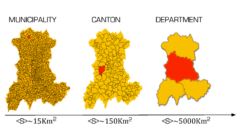
We test this model on 80 case-studies with geographic units of different scales. For example in the same case-study the geographic unit can be either the municipality, the canton or the department, (see an example on Figure 1). More precisely, the case studies include: Czech Republic (municipality scale, 1 case-study), France (municipality scale, 34 case-studies), France (canton scale, 15 case-studies including whole France), France (département scale one case-study (whole France), Italy (municipality scale, 10 case-studies), Italy (province scale, 4 case-studies), USA (county level, 15 case-studies including whole USA). For a detailed description of the datasets see the Appendix.

We show that the single parameter of our model follows a simple universal law that depends only on the average surface of the considered geographic units. This implies that, given the number of commuters in and out of each geographic unit and their average surface, we can derive the whole matrix of flows with a very good confidence.

Figure 1: Three scales of geographic units (Auvergne region, France).

Two other approaches Balcan2009 ; Simini2012 claim to catch universal properties of commuting networks. We show that our model yields significantly more accurate results, especially for case-studies with small geographic units (e.g. municipalities).

The model

We consider the basic double-constrained model setup, without adding any ingredient about the job market characteristics (professions, salary range, etc.). Instead of solving analytically the optimisation problem, we use an individual based procedure that allocates virtual individuals one by one in the different flows between geographic units, according to a probability that is updated after each allocation.

This individual based approach can deal with less constrained data than the doubly-constrained gravity model that requires the total number of commuters in to be equal to the total number of commuters out. In other words the doubly contrained model can only deal with the flows between the considered geographic units; it cannot take into account the commuting links with destinations outside the case study area. This is a problem when only the numbers of commuters in and out the geographic units are available (and not the complete matrix of the commuting flows), because the data do not distinguish between the flows inside and outside the case study area. It is therefore difficult to estimate the correct data to take as input to the doubly-constrained model in this case. Our approach is more flexible and overcomes this difficulty. It does not require that the total number of commuters in and out to be equal (for more details see Lenormand2012 ), hence it can easily use directly the usually available data on the number of commuters in and out of each geographic unit.

Let $s^{out}_{i}$ and $s^{in}_{j}$ be respectively the global number of commuters starting from unit $u_{i}$ and the global number of commuters arriving in unit $u_{j}$. These numbers are initialised from data and then they are progressively modified by the procedure. More precisely, at each step we select unit $u_{i}$ such that $s^{out}_{i}>0$ at random, and we consider a virtual commuter starting from $u_{i}$. We draw at random the working place $u_{j^{*}}$ of this individual among all possible destinations $u_{j}$ according to probabilities $P_{i\rightarrow j}$:

$$P_{i\rightarrow j}=\frac{s^{in}_{j}e^{-\beta D_{ij}}}{\sum_{k=1}^{N}s^{in}_{k}e^{-\beta D_{ik}}}$$ (1)

where $D_{ij}$ is the Euclidian distance in meter between units $u_{i}$ and $u_{j}$ (computable from the Lambert or GIS coordinates). Having drawn $u_{j^{*}}$, we decrement of one $s^{out}_{i}$ and $s^{in}_{j^{*}}$. Note that decrementing $s^{in}$ and $s^{out}$ at each step complicates significantly the derivation of an analytical expression of the model. We chose a probability decreasing exponentially with the distance, in accordance with the investigations carried out in Lenormand2012 and with the literature on commuting network models. The importance of the distance in the commuting choices is embedded in parameter $\beta$: for $\beta\rightarrow 0$ the probability tends to be independent from the distance, while for high values of $\beta$, the probability tends to zero very rapidly when the distance increases, independently from the number of commuters arriving in the units.

To reduce the border effect (see Lenormand2012 ), we consider the job-search basin in an extended (EXT) area, composed by the $n$ residential units and $m$ units surrounding the area. Thus, we have $n$ units which are commuting origins and $N=n+m$ units that are commuting destinations. The generated network is saved in matrix $\tilde{T}\in M_{n\times N}(\mathbb{N})$ where each entry $\tilde{T}_{ij}$ represents the number of commuters between units $u_{i}$ and $u_{j}$. The algorithm is summarized in Algorithm 1.

List of Algorithms 1 Commuting generation model

$D\in\mathrm{M}_{n\times N}(\mathbb{R})$, $s^{in}\in\mathbb{N}^{N}$, $s^{out}\in\mathbb{N}^{n}$, $\beta\in\mathbb{R}_{+}$

$\tilde{T}\in\mathrm{M}_{n\times N}(\mathbb{N})$

$\tilde{T}_{ij}\leftarrow 0$

while $\sum_{k=1}^{n}s^{out}_{k}>0$ do

   Pick at random $i\in|[1,n]|$, such that $s^{out}_{i}\neq 0$

   Pick at random $j$ from $|[1,N]|$

       with a probability $P_{i\rightarrow j}$

   $\tilde{T}_{ij}\leftarrow\tilde{T}_{ij}+1$

   $s^{in}_{j}\leftarrow s^{in}_{j}-1$

   $s^{out}_{i}\leftarrow s^{out}_{i}-1$

end while

Results

A universal law ruling parameter $\beta$

The model depends on a single parameter ruling the importance of the distance in commuting choice. We show that this parameter can be derived as a function of the scale of the problem, independently from the socio-geographical location of the case study area. This opens the possibility to reconstruct the commuting flows (origin-destination matrix) when they are not provided.

We calibrated parameter $\beta$ by maximising the common part of commuters (CPC), based on the Sørensen index Sorensen1948 .

$$CPC(T,\tilde{T})=\frac{2NCC(T,\tilde{T})}{NC(T)+NC(\tilde{T})}$$ (2)

with:

$$NCC(T,\tilde{T})=\sum_{i=1}^{n}\sum_{j=1}^{n}\min(T_{ij}\tilde{T}_{ij})$$ (3)

and

$$NC(T)=\sum_{i=1}^{n}\sum_{j=1}^{n}T_{ij}$$ (4)

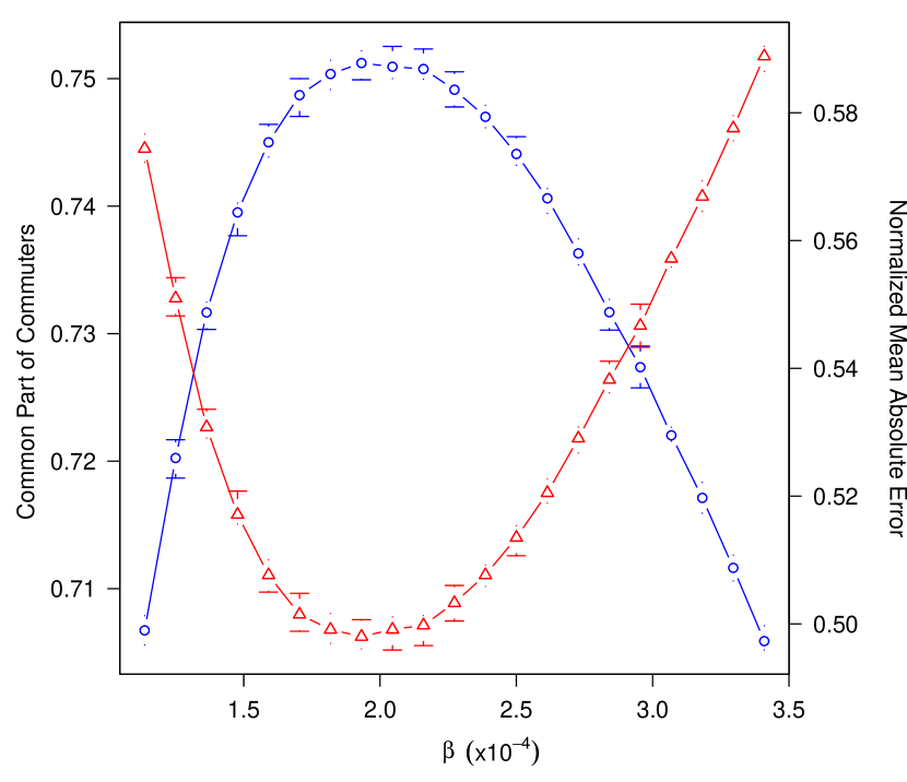
where $T$ is the observed origin-destination matrix and $\tilde{T}$ is the simulated one. This is a similarity measure based on the Sørensen index in ecology computing which part of the commuting flows is correctly reproduced, on average, by the simulated network. It varies between 0, when no agreement is found, and 1, when the two networks are identical. We priviledged this indicator because of its direct interpretation. Indeed, when $NC(T)\simeq NC(\tilde{T})$ (it is the case for our model), the CPC represents the percentage of commuting connection correctly located (i.e. with the right pair origin - destination). Moreover, we tested on all case studies that the results obtained with the MAE, the RMSE or CPC are equivalent (see the Appendix for more details). We have also shown in Gargiulo2012 ; Lenormand2012 that the value of $\beta$ yielding the maximum CPC also yields the maximum similarity between observed and simulated commuting distance distributions. As an example on the $FR1$ case study, Figure 2 shows that the same $\beta$ value maximizes the CPC and minimizes the MAE. In this Figure we can also note that the CPC is very sensitive to $\beta$ and that its value does not vary much with the different replicas of the stochastic solving process.

Figure 2: Plot of the average CPC (blue circle) and the average NMAE (red triangle) in term of $\beta$ for 10 replications of the model for the Auvergne case study (FR1). The error bars represent the minimum value and maximum value obtain over the 10 replications.

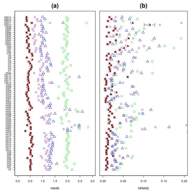
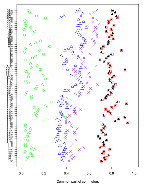
Moreover, in order to have an idea of the improvement of the model compared with complete randomness, we have computed the CPC of a random model where the probabilities presented in Equation (1) are uniform ($P_{i\rightarrow j}=\frac{1}{n}$, where $n$ is the number of units). As shown on the Figure 4 we obtained an average CPC around 0.1. For our model, the CPC is always higher than 0.7 with an average around 0.8, which can be interpreted as 70 to 80 % of correctly predicted commuting connections.

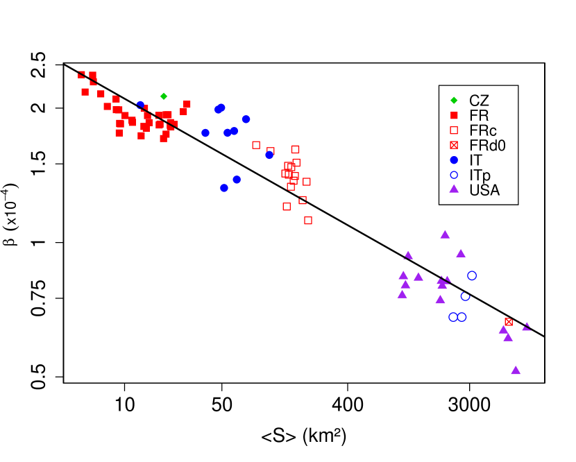
Our goal is to derive the value of $\beta$ from some easily available global characteristics of the case-study, giving the possibility to reconstruct the commuting flows when they are not available. Figure 3 gives strong evidence of such a universal relation.

The x-axis represents the average surface of the geographic units of the case-study ($\langle S\rangle$ in logarithm scale) and the y-axis the optimal $\beta$ value (in logarithm scale). The linear regression in the log-log plane shows a simple relation:

$$\beta=\alpha\langle S\rangle^{-\nu}$$ (5)

with $\alpha=3.15\cdot 10^{-4}$ and $\nu=0.177$. $\alpha$ corresponds to the $\beta$ value for the unitary surface 1 $km^{2}$. The high value of the adjusted $R^{2}=0.92$ confirms the quality of the linear model. We observe that $\beta$ decreases with the average surface of the units $\langle S\rangle$, meaning that, when $\langle S\rangle$ is small (e.g. for municipalities in France) the distance is more important in the commuting choice than when $\langle S\rangle$ is large (e.g. for regions or counties).

Figure 3: Log-log scatter plot of the calibrated $\beta$ values in terms of average surface of the geographic units for 80 case-studies; the line represents the regression line predicting $\beta$.

Figure 4: Common part of commuters (CPC) for the 80 case-studies. The red squares represent the CPC obtained with the value of $\beta$ optimised from data on the case-study network. Black plain triangles represent the average CPC obtained with $\beta$ values estimated with the rule linking $\beta$ and the average surface of the units obtain with the cross-validation; Dark bars represent the minimum and the maximum CPC obtained with the estimated $\beta$ but in most cases they are too close to the average to be seen. The green circles represent the CPC obtained with the random model. The blue triangles represent the CPC obtained with the radiation model. The purple crosses represent the CPC obtained with the modified version of the radiation model.

We now evaluate the robustness of our estimation of $\alpha$ and $\nu$ using a common statistical procedure: the cross-validation. The cross-validation aims at evaluating the potential error of using the $\beta$ value derived from the regression model intsead of deriving this value by optimisation for a new case study. This procedure repeats a large number of times the following steps: define a sub-sample of the total sample of case studies, derive a regression model of $\beta$ from this sub-sample, for each case study that do not belong to the sub-sample, derive $\beta$ from this regression model and compare the corresponding CPC with the value of $\beta$ directly calibrated on the complete origin - destination data. The dataset (including 80 case-studies) is randomly cut into two sets, called the training set (comprising 53 case-studies) and the test set (composed of 27 case-studies). We build a regression model on the training set, providing $\alpha$ and $\nu$, from which we derive estimates of $\beta$ for each of the 27 case-studies of the testing set. We have 27 estimations of $\beta$ using the relation 5 where $\alpha$ and $\nu$ are obtained from the random sub-sample of 53 case-studies. We repeat this process $10,000$ times obtaining 270,000 estimations of $\beta$ (uniformly distributed over the 80 case-studies) corresponding to about $\frac{270,000}{80}=3,375$ estimations of $\beta$ for each case study. Then we calculate the average, minimum and maximum CPC for each of these values of $\beta$, and we compare them with the CPC obtained with value of $\beta$ directly calibrated on the data.

Figure 4 shows, for each case-study, the CPC associated with the calibrated $\beta$, the average CPC obtained with the $\beta$ values estimated from the cross-validation and the confidence interval defined by the minimum and the maximum values (but it is too small to be seen in most cases). The CPC obtained with the calibrated $\beta$ value (black triangle) is almost the same as the average CPC obtained with the estimated $\beta$ in most cases (red square). Globally, we can conclude that the $\beta$ estimated with the log-linear model and the calibrated $\beta$ lead to very similar CPCs and also very similar MAE and the RMSE as shown in the Appendix. The method appears therefore fairly robust and this gives confidence for using it with the value of $\beta$ derived from our loglog regression in new cases studies.

Figure 5: Comparing the predictions of the radiation model with ours for two case studies, the first row ((a)-(c)) for USA0 (USA at county scale) and the second row ((d)-(f)) for FR1 (Auvergne region, France at municipality scale). Plots (a), (b) , (d) and (e): Comparison between the observed (Census) and the simulated (model) non-zero flows. Grey points are the scatter plot for each pair of units. The boxplots (D1, Q1, Q2, Q3 and D9) represent the distribution of the number of simulated travelers in different bins of number of observed travelers. The blue circles represent the average number of simulated travelers in the different bins. Plots (c) and (f): Commuting distance distributions (km) (i.e. Probability for a commuters of the region to commut at a distance $d$). The blue line represents the observed data, the red one the results of our model and the green one the results of the radiation model.

Comparaison with other universal derivations of commuting networks

Two other different approaches, Balcan2009 and Simini2012 , claim also to provide a universal derivation of commuting networks. The objective of Balcan2009 is to generate a worldwide commuting network, and the model must deal with the wide variety of populations and surfaces of geographic units for which the data are available. To solve this difficulty, the authors project these data on ad-hoc units defined with a Voronoi diagram. They define their basic unit as a cell approximately equivalent to a rectangle of 25 x 25 kilometers along the Equator. This allows them to calibrate their model because a unit is the same object whatever the country. This is an interesting solution for generating a world-wide commuting network but it leads to an average commuting distance of 250 km which is much larger than the average distance of daily commuting. For example for the USA case study the average distance of daily commuting is about 68 km for the observed network and about 64 km for the simulated network obtained with our algorithm. For the Auvergne (France) case study at municipality scale the average distance of daily commuting is about 12 km for the observed network and about 11 km for the simulated one.

In the radiation model, proposed in Simini2012 , the commuting flow between two geographic units is a function of the cumulated population in a circle at the distance between the two units. The model has an elegant analytical solution and the average flow $T_{ij}$ from unit $u_{i}$ to unit $u_{j}$ can be approximated by

$$\langle T_{ij}\rangle=\left(m_{i}\frac{P_{c}}{P}\right)\frac{m_{i}n_{j}}{\left(m_{i}+s_{ij}\right)\left(m_{i}+n_{j}+s_{ij}\right)}$$ (6)

where $m_{i}$ and $n_{j}$ are respectively the population of units $u_{i}$ and $u_{j}$, $P_{c}$ is the total number of commuters and $P$ is the total population in the case-study region, and $s_{ij}$ the total population in the circle of radius $r_{ij}$ centred at $u_{i}$ (excluding the source and destination population).

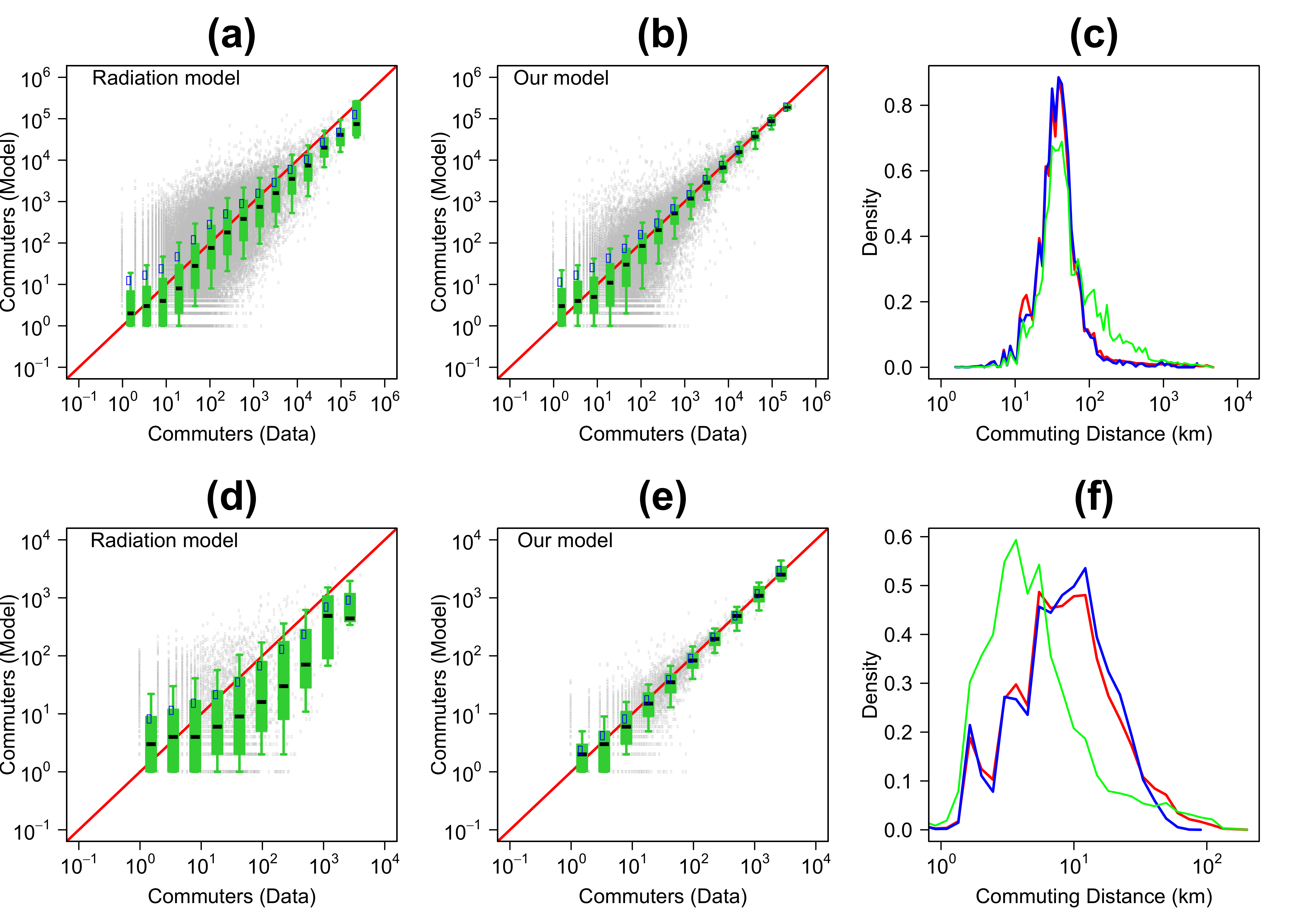
We implemented their analytical approximation and reproduced the graphs presented in their paper. Figure 5 shows the comparison between the radiation model and ours in the US for inter-county commuting and in the French Auvergne region for inter-municipality commuting (see the Appendix for more examples). We observe that in both cases our approach yields significantly better results. Moreover, as shown on Figure 4, the average CPC for the radiation model on all the case studies is around 0.4, and lower for all case studies than the one obtained with our approach.

However, it should be reminded that our model uses more specific data (total number of commuters in and out of each geographic unit) than the radiation model, hence one could expect our results to be more accurate. Therefore, to be fair with the radiation model we implemented a modified version of this model using the number of out and in commuters of each units. This new approximation is presented in Equation 7 where $s_{ij}$ the total number of in-commuters in the circle of radius $r_{ij}$ centred at $u_{i}$ (excluding the source and destination).

$$\langle T_{ij}\rangle=s^{out}_{i}\frac{s^{out}_{i}s^{in}_{j}}{\left(s^{out}_{i}+s_{ij}\right)\left(s^{out}_{i}+s^{in}_{j}+s_{ij}\right)}$$ (7)

As shown on Figure 4, this new model reaches an average CPC around 0.5 which is higher than the original radiation model but still significantly lower than the results obtained with our model. Using the MAE and the RMSE leads to the same conclusions (see the Appendix for more details).

Discussion

The power law of our model’s single parameter $\beta$ with the average area of the case study geographic units, is surprising to us because of the high variety in our case studies in terms of scale, number of units, number of commuters and surface areas. For instance the Auvergne region in France is rural with a population density of about 50 hab./km² whereas the New York City region is very urban with a population density of about 6500 hab./km². As far as we know, this is the first time that a single model is shown to fit such diverse group of datasets.

We show that our approach outperforms the radiation model and that the difference of input data plays a minor role in this superiority. This superiority is not due to our particular treatment of the border effects either. Indeed, we could check our approach outperforms the radiation model also on particular case studies (e.g. on islands such as Corsica) where this border effect does not play. We can conclude that the accuracy of our model comes from a proper use of the number of commuters in and out of each geographic unit and an adequate choice of the function of the distance.

The results of the cross validation procedure give a good confidence in the robustness of this law. However, we have to admit that, despite their diversity, our 80 case studies come all from western industrialised countries. Therefore it will be important to check the validity of our law on case studies coming from other continents and less industrialised countries. Moreover, we use a very rough approximation of the distance between the geographic units with the Euclidian distance between the unit centroids. More accurate approximations of this distance would certainly improve the results. Finally, we also intend to apply our approach to commuting networks inside urban areas because many cities of the world show an impressive growth and an increasing part of commuting takes place within them Roth2011 . An important issue in our perspective is to check if our law holds at this scale.

APPENDIX

Data presentation

Datasets

Commuting data are usually provided by statistical offices in the form of origin-destination tables. We analyzed $80$ case studies from $7$ differents datasets and $4$ different country (described in Table S2). In these appendices we called outside (Out.) the $m$ units surrounding the area.

Distance

The distances between units are Euclidean, computed using the Lambert coordinates or the latitude/longitude of the centroid of the units.

Case studies

We define two types of case studies: from administrative regions and from aggregation of small administrative units around a randomly chosen point. Each case study is composed of a region and an outside (the units surrounding the region at a reasonable distance).

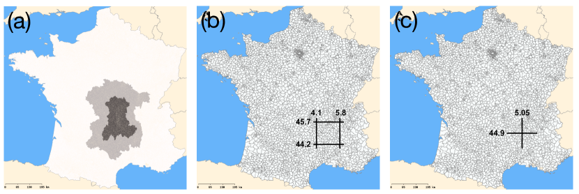
To build a case study from an admistrative region, we select an administrative region (For example the Auvergne region represented by the dark grey region in Figure 1a) and to build the outside we select all the units surrounding the region at a reasonable distance (For the Auvergne region example, the outside is represented by the light grey region in Figure 1a).

To build a case study by aggregation of units, firstly, we define the number of desired units and we draw at random a latitude and a longitude (For example the point represented in Figure 1b). In a second time we gradually increase the area of a square with as center the starting point until the desired number of units is obtained (Figure LABEL:FigureS1c). To build the outside we select all the units surrounding the defined set of units at a reasonable distance or all the remaining units in the country (it depends of the number of units).

The case studies with an identifier with a $0$, for example $FRc0$, are complete network of the country without outside. Indeed, we have no data for the surrounding countries. When we consider a region in the country we can determine the outside as the units surrounding the region. When we consider as a region the whole country we can’t determine an outside, it is the case for $FRc0$ (all the Cantons of France), $Frd0$ (all the Départements of France), $Itp0$ (all the Provincias of Italy) and $USA0$ (all the counties of USA).

Source

The $3$ French datasets are measured for the 1999 French Census by the French Statistical Institute, $INSEE$. They were kindly made available by the Maurice Halbwachs Center. The $2$ Italian datasets are measured for the 2001 Italian Census by the National Institute for Statistics, $ISTAT$.

Table S1: Description of the case studies

Case study	Number of units (area)	Number of units (outside)	Surface (km2)	Average unit surface (km2)	Standard deviation unit surface (km2)	Observed number of commuters (Area)	Estimated number of commuters (Area)
CZ	43	630	35369	822.54	703.23	6585	6847
FR1	1310	3463	26013	19.86	12.49	261822	262452
FR2	1269	1447	27208	21.44	16.14	608587	613363
FR3	419	2809	5762	13.75	8.46	90456	76829
FR4	903	3081	8280	9.17	9.55	409661	402565
FR5	2296	2835	41309	17.99	21.30	679639	657095
FR6	261	3124	5175	19.83	10.46	52921	48681
FR7	185	1859	5167	27.93	18.71	9474	8981
FR8	1464	2467	25810	17.63	12.94	333045	333540
FR9	1842	4718	39151	21.25	14.76	514461	529535
FR10	3020	3845	45348	15.02	15.74	502326	494946
FR11	747	3169	16942	22.68	14.15	118508	117217
FR12	1786	3317	16202	9.07	7.46	239931	236314
FR13	1420	3536	12317	8.67	5.64	396800	402128
FR14	433	3914	6211	14.34	12.41	30175	28729
FR15	515	3808	5874	11.41	9.54	76519	72896
FR16	2339	3067	23547	10.07	7.51	505807	507812
FR17	260	1814	5565	21.40	13.15	17310	17071
FR18	1545	3046	27367	17.71	15.78	354824	354566
FR19	1948	1983	25606	13.14	12.94	333045	329908
FR20	36	1245	176	4.89	3.28	193236	182808
FR21	262	1543	2284	8.72	6.62	226205	206624
FR22	185	1707	1246	6.74	3.83	143938	124185
FR23	47	1234	245	5.21	3.03	143586	121474
FR24	377	2283	3525	9.35	7.44	160294	157123
FR25	195	2338	3718	19.07	17.66	26576	24975
FR26	547	449	4116	7.52	15.87	59709	61324
FR27	163	353	4299	26.37	27.53	145995	148922
FR28	327	2788	4781	14.62	9.76	134048	130910
FR29	102	2031	609	5.97	4.21	22520	20549
FR30	40	783	236	5.90	4.28	139181	125542
FR31	196	1597	1804	9.20	6.04	188855	165505
FR32	463	2588	5229	11.29	8.03	50505	51413
FR33	433	2728	6004	13.87	9.07	69377	63078
FR34	286	2088	5857	20.48	13.36	38141	37197
FRc0	3646	0	540241	171.72	99.90	12193161	12193161
FRc1	1062	2584	173797	163.65	91.23	2229003	2265247
FRc2	523	3123	58366	111.60	114.44	3892543	3922481
FRc3	226	3420	33041	146.20	70.56	548048	558086
FRc4	160	3486	25044	156.52	75.47	320432	323169
FRc5	55	3591	7847	142.67	71.64	61761	60285
FRc6	869	2777	131174	150.95	96.62	1995302	1983097
FRc7	2088	1558	351073	168.14	94.18	4459338	4523902
FRc8	100	3546	20246	202.46	161.41	307744	316592
FRc9	600	3046	113905	189.84	103.57	1078183	1095993
FRc10	302	3344	26627	88.17	77.64	1306425	1274670
FRc11	906	2740	142619	157.42	100.21	2324444	2358580
FRc12	1500	2146	250676	167.12	99.00	3224586	3284517
FRc13	32	3614	6653	207.91	145.33	11959	10634
FRc14	506	3140	75603	149.41	85.63	1311912	1331984
FRd0	94	0	540250	5747.35	1957.11	3548178	3548178
IT1	377	0	24090	63.90	61.89	225351	225351
IT2	395	201	24157	61.16	77.51	409889	408692
IT3	1002	2020	54918	54.81	71.37	1235378	1193338
IT4	201	507	14964	74.45	82.42	246609	248562
IT5	204	1005	10567	51.80	55.68	279014	272310
IT6	51	506	5582	109.45	101.52	57446	51211
IT7	2000	4001	98693	49.35	60.97	2849914	2812238
IT8	186	1023	2412	12.97	15.25	316602	286285
IT9	1510	4004	71167	47.13	58.08	1703944	1702002
IT10	705	3008	26809	38.03	41.62	401998	403307
ITp0	99	0	277220	2800.20	1619.86	1567576	1567576
ITp1	50	49	131773	2635.45	1401.23	742229	727038
ITp2	30	69	93666	3122.21	1599.56	266696	272316
ITp3	20	79	45854	2292.72	1128.38	264824	259988
USA0	3108	0	8070785	2596.78	3437.29	34077841	34077841
USA1	1015	2093	1876151	1848.42	916.86	5855813	5902784
USA2	103	3005	101411	984.57	341.47	527136	535608
USA3	54	3054	306284	5671.93	4488.99	604043	597371
USA4	2011	1097	4169235	2073.21	1786.40	14767588	14926726
USA5	202	2906	404093	2000.46	1994.32	8789633	8893748
USA6	504	2604	949238	1883.41	1041.57	2125887	2155981
USA7	806	2302	4234740	5254.02	5626.18	5003104	5099317
USA8	352	2756	2723212	7736.40	7741.02	4147054	4234376
USA9	1507	1601	2877429	1909.38	1517.28	10099598	10234438
USA10	13	3095	14123	1086.37	343.73	58212	53513
USA11	32	3076	205989	6437.17	4105.95	22496	24085
USA12	1004	2104	1292835	1287.68	563.79	9704950	9735646
USA13	207	2901	207785	1003.79	352.24	1307774	1326018
USA14	301	2807	312955	1039.72	394.71	2054878	2085408

Results with standard indicators of error

We computed the results with standard indicators of error.

• The Normalized Mean Absolute Error:

  $$NMAE(T,\tilde{T})=\frac{\sum_{i=1}^{n}\sum_{j=1}^{n}|T_{ij}-\tilde{T}_{ij}|}{\sum_{i=1}^{n}\sum_{j=1}^{n}T_{ij}}$$ (8)

• Normalized Root Mean Square Error:

  $$NRMSE(T,\tilde{T})=\frac{\sqrt{\sum_{i=1}^{n}\sum_{j=1}^{n}(T_{ij}-\tilde{T}_{ij})^{2}}}{\sum_{i=1}^{n}\sum_{j=1}^{n}T_{ij}}$$ (9)

Table S2: Presentation of the datasets. * Data are available online at http://www.czso.cz/eng/redakce.nsf/i/home and ** Data are available online at http://www.census.gov/geo/www/gazetteer/places2k.html

Dataset	Country	Case Study	Distance	Region	Scale	Year	Source
1	Czech Republic	CZ	Latitude Longitude	Administrative	Municipality	2001	*
2	France	FR1 - FR34	Lambert	Administrative	Municipality	1999	INSEE
3	France	FRc0 - FR14	Latitude Longitude	Arbitrary aggregation	Canton	1999	INSEE
4	France	FRd0	Latitude Longitude	Administrative	Département	1999	INSEE
5	Italy	IT1 - IT10	Latitude Longitude	Arbitrary aggregation	Municipality	2001	ISTAT
6	Italy	ITp0 - ITp4	Latitude Longitude	Arbitrary aggregation	Provincia	2001	ISTAT
7	USA	USA0 - USA14	Latitude Longitude	Arbitrary aggregation	County	2000	**

Figure S1: Maps to illustrate the build process regions. (a) Administrative; (b) starting point of aggregation and (c) limits of aggregated units. Base maps source: Cemagref - DTM - Développement Informatique Système d’Information et Base de Données : F.Bray & A.TorreIGN (Géofla^®,2007).

Figure S2: Normalized Mean Absolute Error (a) and Normalized Root Mean Square Error (b) for the 80 case-studies. The red squares represent the errors obtained with the value of $\beta$ optimised from data on the case-study network. Black plain triangles represent the average errors obtained with $\beta$ values estimated with the rule linking $\beta$ and the average surface of the units obtain with the cross-validation; Dark bars represent the minimum and the maximum errors obtained with the estimated $\beta$ but in most cases they are too close to the average to be seen. The green circles represent the errors obtained with the random model. The green circles represent the errors obtained with the random model. The blue triangles represent the value obtained with the radiation model. The purple cross represent the errors obtained with the modified version of the radiation model.

References

- [1] D. Balcan, V. Colizza, B. Goncalves, H. Hud, J.J. Ramasco, and A. Vespignani. Multiscale mobility networks and the spatial spreading of infectious diseases. Proceedings of the National Academy of Sciences of the United States of America, 106(51):21484–21489, 2009.
- [2] F. Simini, M. C. Gonzalez, A. Maritan, and A.-L. Barabasi. A universal model for mobility and migration patterns. Nature, advance online publication:–, February 2012.
- [3] J.D. Ortúzar and L.G. Willumsen. Modeling Transport. John Wiley and Sons Ltd, New York, 2011.
- [4] A. De Montis, M. Barthelemy, A. Chessa, and A. Vespignani. The structure of interurban traffic: A weighted network analysis. Environment and Planning B: Planning and Design, 34(5):905–924, 2007.
- [5] A. De Montis, A. Chessa, M. Campagna, S. Caschili, and G. Deplano. Modeling commuting systems through a complex network analysis: A study of the italian islands of sardinia and sicily. The Journal of Transport and Land Use, 2(3):39–55, 2010.
- [6] M. Barthelemy. Spatial networks. Physics Reports, 499:1–101, 2011.
- [7] J. Rouwendal and P. Nijkamp. Living in two worlds: A review of home-to-work decisions. Growth and Change, 35(3):287–303, 2004.
- [8] A. G. Wilson. Land-use/transport interaction models: Past and future. Journal of Transport Economics and Policy, 32(1):pp. 3–26, 1998.
- [9] J.-M. Choukroun. A general framework for the development of gravity-type trip distribution models. Regional Science and Urban Economics, 5(2):177–202, 1975.
- [10] J.J. de Vries, P. Nijkamp, and P. Rietveld. Exponential or power distance-decay for commuting? an alternative specification. Environment and Planning A, 41(2):461–480, 2009.
- [11] A.S. Fotheringham. Spatial structure and distance-decay parameters. Annals, Association of American Geographers, 71(3):425–436, 1981.
- [12] F. Gargiulo, M. Lenormand, S. Huet, and O. Baqueiro Espinosa. Commuting network model: getting to the essentials. Journal of Artificial Societies and Social Simulation, 15(2):13, 2012.
- [13] M. Lenormand, S. Huet, and F. Gargiulo. Generating french virtual commuting network at municipality level. 2012.
- [14] T. Sørensen. A method of establishing groups of equal amplitude in plant sociology based on similarity of species and its application to analyses of the vegetation on danish commons. Biol. Skr., 5:1–34, 1948.
- [15] C. Roth, S. M. Kang, M. Batty, and M. Barthelemy. Structure of urban movements: Polycentric activity and entangled hierarchical flows. PLoS ONE, 6(1), 01 2011.