Optimal estimates of the diffusion coefficient of a single Brownian trajectory

Abstract

Modern developments in microscopy and image processing are revolutionizing areas of physics, chemistry and biology as nanoscale objects can be tracked with unprecedented accuracy. The goal of single particle tracking is to determine the interaction between the particle and its environment. The price paid for having a direct visualization of a single particle is a consequent lack of statistics. Here we address the optimal way of extracting diffusion constants from single trajectories for pure Brownian motion. It is shown that the maximum likelihood estimator is much more efficient than the commonly used least squares estimate. Furthermore we investigate the effect of disorder on the distribution of estimated diffusion constants and show that it increases the probability of observing estimates much smaller than the true (average) value.

I Introduction

Single particle tracking dates back to the classic study of Perrin on Brownian motion (BM) perrin . It generates the position time series of an individual particle trajectory ${\bf B}(t)$ in a medium (see, e.g., Refs. bra ; saxton ) and when properly interpreted, the information drawn from a single, or a finite number of trajectories, can provide insight into the mechanisms and forces that drive or constrain the motion of the particle. The method is thus potentially a powerful tool to probe physical and biological processes at the level of a single molecule moerner . At the present time, single particle tracking is widely used to characterize the microscopic rheological properties of complex media mason , and to probe the active motion of biomolecular motors greenleaf . In biological cells and complex fluids, single particle trajectory (SPT) methods have, in particular, become instrumental in demonstrating deviations from normal BM of passively moving particles (see, e.g., Refs. golding ; weber ; bronstein ; seisenberger ).

The reliability of the information drawn from SPT analysis, obtained at high temporal and spatial resolution but at expense of statistical sample size is not always clear. Time averaged quantities associated with a given trajectory may be subject to large fluctuations among trajectories. For a wide class of anomalous diffusions described by continuous-time random walks, time-averages of certain particle’s observables are, by their very nature, themselves random variables distinct from their ensemble averages rebenshtok . An example is the square displacement time-averaged along a given trajectory, which differs from the ensemble averaged mean squared displacement he . By analyzing time-averaged displacements of a particular trajectory realization, subdiffusive motion can actually look normal, although with strongly differing diffusion coefficients from one trajectory to another lubelski .

Standard BM is a much simpler and exceedingly well-studied random process yuval than anomalous diffusion, but still it is far of being as straightforward as one might be tempted to think. Even in bounded systems, despite the fact that the first passage time distribution has all moments, first passages to a given target of two independent identical BMs, starting at the same point in space, will most likely occur at two distinctly different time moments carlos , revealing a substantial manifestation of sample-to-sample fluctuations. Ergodicity, that is, equivalence of time- and ensemble-averages of square displacement holds only in the infinite sample size limit. In practice, it means that standard fitting procedures applied to finite (albeit very long) trajectories of a given particle will unavoidably lead to fluctuating estimates of the diffusion coefficient $D$. Indeed, variations by orders of magnitude have been observed in SPT measurements of the diffusion coefficient of the LacI repressor protein along elongated DNA austin (see also Section VI.1). Significant sample-to-sample fluctuations resulting in broad histograms for the value of the diffusion coefficient have been observed experimentally for two-dimensional (2D) diffusion in the plasma membrane saxton , as well as for diffusion of a single protein in the cytoplasm and nucleoplasm of mammalian cells goulian .

Such a broad dispersion of the value of the diffusion coefficient extracted from SPT measurements, raises important questions about the correct or optimal methodology that should be used to estimate $D$. Indeed, these measurements are performed in rather complex environments and each SPT has its own history of encounters with other species, defects, impurities, etc., which inevitably results in rather broad histograms for observed $D$. On the other hand, it is highly desirable to have a reliable estimator of the diffusion coefficient even for the hypothetical ”pure” cases, such as, e.g., unconstrained standard BM. A reliable estimator should produce a distribution of $D$ as narrow as possible and with the most probable value as close as possible to the ensemble average one. A knowledge of the distribution of such an estimator could provide a useful gauge to identify effects of the medium complexity as opposed to variations in the underlying thermal noise driving microscopic diffusion. Commonly used methods of extraction of $D$ from the SPT data are based on a least square (LS) estimate of the time-averaged square displacement and some of its derivatives (see, e.g., saxton ; goulian ; saxton2 and the next section). A recent study, Ref. boyer , focussed on estimators for $D$ for 1D BM, the statistics of which is amenable to analytical analysis. Several methods for estimating $D$ from the SPT data were studied and it was shown that a completely different approach - consisting of maximizing the unconditional probability of observing the whole trajectory - is superior to those based on the LS minimization. As a matter of fact, at least in 1D systems the distribution of the maximum likelihood (ML) estimator of the diffusion coefficient not only appears narrower than the LS ones, resulting in a smaller dispersion, but also the most probable value of the diffusion coefficient appears closer to the ensemble average $D$ boyer .

In this paper we focus first on the case of pure standard BM and calculate exactly, for arbitrary spatial dimension $d$, the distribution $P(u)$ of the maximum likelihood estimator

$$u=\frac{1}{T}\int^{t_{0}+T}_{t_{0}}dt\frac{{\bf B}^{2}(t)}{\mathbb{E}\left\{{\bf B}^{2}(t)\right\}},$$ (1)

of the diffusion coefficient of a single BM trajectory ${\bf B}(t)$. The parameter $t_{0}$ here is the lag time (at which the measurement is started) which can be set equal to zero for standard BM without any lack of generality. However for anomalous diffusion, or BM in presence of disorder $t_{0}$ will play a significant role. The symbol $\mathbb{E}\{\ldots\}$ denotes ensemble average, so that

$$\mathbb{E}\left\{{\bf B}^{2}(t)\right\}=2dDt\,,$$ (2)

$D$ being the ensemble-average diffusion coefficient. Consequently, the random variable $u$ is defined as the ratio of the realization-dependent diffusion coefficient, calculated as the weighted time-average along a single trajectory, and the ensemble average diffusion coefficient. Clearly, $\mathbb{E}\left\{u\right\}\equiv 1$.

Further on, we analyze here a useful measure of sample-to-sample fluctuations - the distribution function $P(\omega)$ of the random variable

$$\omega=\frac{u_{1}}{u_{1}+u_{2}},$$ (3)

where $u_{1}$ and $u_{2}$ are two identical independent random variables with the distribution $P(u)$. Hence, the distribution $P(\omega)$ probes the likelihood of the event that the diffusion coefficients drawn from two different trajectories are equal to each other.

Finally, we discuss the effect of disorder on the distributions $P(u)$ and $P(\omega)$ for 1D BM in random media. We consider two different models of diffusion in 1D random environments - diffusion in presence of a random quenched potential with a finite correlation length, as exemplified here by the Slutsky-Kardar-Mirny model slutsky , and diffusion in a random forcing landscape - the so-called Sinai model Sinai1982 . The former is appropriate for diffusion of proteins on DNA, which is affected by the base-pair reading interaction and thus is sequence dependent, while the latter describes, for example, the dynamics of the helix-coil boundary in a melting heteropolymer pgg . Note that in the former case, at sufficiently large times, one observes a diffusive-type motion with $B_{t}^{2}\sim t$, while in the latter case dynamics is strongly anomalous so that $B_{t}$ is logarithmically confined, $B_{t}^{2}\sim\ln^{4}t$.

The paper is outlined as follows: In Section II we recall some common fitting procedures used to calculate the diffusion coefficient from single particle tracking data. In Section III we focus on the maximum likelihood estimator and, generalizing the approach developed in Ref. boyer for 1D systems, obtain new results for the moment generating function $\Phi(\sigma)$ and the probability density function $P(u)$ of the ML estimator for arbitrary spatial dimension $d$. In that Section we also obtain the asymptotical behavior of the probability distribution function $P(u)$, as well as its kurtosis and skewness. Next, in Section IV we focus on the probability distribution function of the random variable $\omega$ - a novel statistical diagnostics of the broadness of the parental distribution $P(u)$ which probes the likelihood of the event that two estimates of the diffusion coefficient drawn from two different trajectories are the same. Further on, Section V presents a comparison of the commonly used least squares estimator and the maximum likelihood estimator. We show that the latter outperforms the former in any spatial dimension $d$ producing a lower variance and the most probable value being closer to the ensemble average value. Next, in Section VI we focus on Brownian motion in presence of disorder. As exemplified by two models of dynamics in systems with quenched disorder - Sinai diffusion (random force) and Slutsky-Kardar-Mirny model (random potential), disorder substantially enhances the importance of sample-to-sample fluctuations. We show that the observation of values of the diffusion coefficient significantly lower than the ensemble average becomes more probable. We show, as well, that as the strength of disorder is increased, the distribution $P(\omega)$ undergoes a surprising shape-reversal transition from a bell-shaped unimodal to a bimodal form with a local minimum at $\omega=1/2$. Finally, we conclude in Section VII with a brief recapitulation of our results and some outline of our further research.

II Fits for the diffusion coefficient of a single trajectory

To set up the scene, we first briefly recall several fitting procedures commonly used to calculate the diffusion coefficient from the SPT data. More detailed discussion can be found in Refs. saxton ; goulian ; saxton2 ; boyer . We focus here on estimators which yield a first power of $D$. Non-linear estimators, e.g. a mean maximal excursion method ralf which has been used to study anomalous diffusion and produces $\sqrt{D}$, will be analyzed elsewhere.

One of the simplest methods consists in calculating a least squares estimate based on the minimization of the integral

$$\int^{T}_{0}dt\left({\bf B}^{2}(t)-l(t)\right)^{2},$$ (4)

where the diffusion law $l(t)$ is taken either as a linear, $l(t)=2dD_{l}t$, or an affine function, $l(t)=2dD_{a}t+b_{a}$. In particular, for the linear case the least squares minimization yields the following linear-least-squares estimator:

$$u_{ls}=\frac{A}{T}\int^{T}_{0}dt\,t\,{\bf B}^{2}(t),$$ (5)

where $A$ is the normalization factor, $A=3/2dDT^{2}$, conveniently chosen so that $\mathbb{E}\left\{u_{ls}\right\}\equiv 1$.

A second, more sophisticated, approach is based on

$$\delta^{2}_{T}(t)=\frac{1}{T-t}\int^{T-t}_{0}\,dt^{\prime}\,\left({\bf B}(t^{\prime}+t)-{\bf B}(t^{\prime})\right)^{2}\,,$$ (6)

which is the temporal moving average over a sufficiently long trajectory ${\bf B}(t)$ produced by the underlying process of duration $T\gg t$. The diffusion coefficient is then extracted from fits of $\delta^{2}_{T}(t)$, or from a related least squares estimator, which is given by the following functional of the trajectory

$$u_{\delta}=\frac{A}{T}\int^{T}_{0}\,dt\,t\,\delta^{2}_{T}(t),$$ (7)

where $A$ is the same normalization constant as in Eq. (5). Note that the random variable $u_{\delta}$ is again conveniently normalized so that $\mathbb{E}\left\{u_{\delta}\right\}\equiv 1$, which enables a direct comparison of the respective distributions of different estimators. As shown in Ref. boyer , $u_{\delta}$ only provides a slightly better estimate of $D$ than $u_{ls}$. A conceptually different fitting procedure has been discussed in Ref. boyer which amounts to maximizing the unconditional probability of observing the whole trajectory ${\bf B}(t)$, assuming that it is drawn from a Brownian process with mean-square displacement $2dDt$ (see Eq. (2)). This is the maximum likelihood estimate which takes the value of $D$ that maximizes the likelihood of ${\bf B}(t)$, defined as:

$$L=\prod_{t=0}^{T}\left(4\pi dDt\right)^{-d/2}\exp\left(-\frac{{\bf B}^{2}(t)}{4dDt}\right)$$ (8)

where the trajectory ${\bf B}(t)$ is appropriately discretized. Differentiating the logarithm of $L$ with respect to $D$ and setting $d\ln L/dD=0$, one finds the maximum likelihood estimate of $D$, which upon a proper normalization is defined by Eq. (1).

Below we will derive the distribution function $P(u)$ of the ML estimator $u$ and compare it against numerical results for the distribution function of the LS estimator $u_{\delta}$ for $d=1,2,3$.

III Distribution of the ML estimator

III.1 The moment generating function

Let $\Phi(\sigma)$ denote the moment generating function of the random variable $u$ defined in Eq. (1),

$$\Phi(\sigma)=\mathbb{E}\left\{e^{-\sigma u}\right\}.$$ (9)

The squared distance from the origin, of $d$-dimensional BM at time $t$ for a given realization, decomposes into the sum

$${\bf B}^{2}(t)=\sum_{i=1}^{d}B_{i}^{2}(t),$$ (10)

$B_{i}(t)$ being realizations of trajectories of independent 1D BMs (for each spatial direction). Thus, $\Phi(\sigma)$ factorizes

$$\Phi(\sigma)=G^{d}(\sigma),$$ (11)

where

$$G(\sigma)=\mathbb{E}\left\{\exp\left(-\frac{\sigma}{2dDT}\int^{T}_{0}d\tau\frac{B_{i}^{2}(\tau)}{\tau}\right)\right\}.$$ (12)

Here, in order to calculate $G(\sigma)$, we follow the strategy of Ref. boyer and introduce an auxiliary functional:

$$\Psi(x,t)=\mathbb{E}^{x}_{t}\left\{\exp\left(-\frac{\sigma}{2dDT}\int^{T}_{t}d\tau\frac{B_{i}^{2}(\tau)}{\tau}\right)\right\}$$ (13)

where the expectation is for a BM starting at $x$ at time $t$. We derive a Feynman-Kac type formula for $\Psi(x,t)$ considering how the functional in Eq. (13) evolves in the time interval $(t,t+dt)$. During this interval the BM moves from $x$ to $x+dB_{i}(t)$, where $dB_{i}(t)$ is an infinitesimal Brownian increment such that $\mathbb{E}_{dB}\{dB_{i}(t)\}=0$ and $\mathbb{E}_{dB}\{dB^{2}_{i}(t)\}=2Ddt$, where $\mathbb{E}_{dB}$ denotes now averaging with respect to the increment $dB_{i}(t)$. For such an evolution we have to order $dt$:

$$\Psi(x,t) = \mathbb{E}\Big{\{}\left(1-\frac{\sigma x^{2}}{2dDTt}dt\right)$$ (14)

$$\times \mathbb{E}^{x+dB_{i}(t)}_{t+dt}\left\{\exp\left(-\frac{\sigma}{2dDT}\int^{T}_{t+dt}d\tau\frac{B_{i}^{2}(\tau)}{\tau}\right)\right\}\Big{\}}$$

$$= \mathbb{E}\left\{\Psi(x+dB_{i}(t),t+dt)\left(1-\frac{\sigma x^{2}}{2dDTt}dt\right)\right\}$$

Expanding the right-hand-side of the latter equation to second order in $dB_{i}(t)$, linear order in $dt$ and performing averaging, we find eventually the following Schrödinger equation:

$$\frac{\partial\Psi(x,t)}{\partial t}=-D\frac{\partial^{2}\Psi(x,t)}{\partial x^{2}}+\frac{\sigma x^{2}}{2dDTt}\Psi(x,t).$$ (15)

The solution of this equation has been obtained in Ref. boyer and gives

$$G(\sigma)=\Psi(0,0)=\left(I_{0}\left(\sqrt{8\sigma/d}\right)\right)^{-1/2},$$ (16)

where $I_{0}(.)$ is the modified Bessel function abramowitz . Consequently, we find the following general result

$$\Phi(\sigma)=\left(I_{0}\left(\sqrt{8\sigma/d}\right)\right)^{-d/2}.$$ (17)

Note that $\Phi(\sigma)$ is independent of $T$ and $D$, as it should in virtue of the scaling properties of the BM.

III.2 The distribution function

We turn next to the analysis of the distribution of the ML estimator defined in Eq. (1). First of all, we calculate several first moments of $u$ by merely differentiating the result in Eq. (17):

$$\mathbb{E}\left\{u^{2}\right\} = 1+\frac{1}{d}$$

$$\mathbb{E}\left\{u^{3}\right\} = 1+\frac{3}{d}+\frac{8}{3d^{2}}$$

$$\mathbb{E}\left\{u^{4}\right\} = 1+\frac{6}{d}+\frac{41}{3d^{2}}+\frac{11}{d^{3}}$$ (18)

Consequently, one may expect that all moments tend to $1$ as $d\to\infty$, so that $P(u)\to\delta(u-1)$. For fixed $d$, the variance $\mathbb{E}\left\{u^{2}\right\}-\mathbb{E}\left\{u\right\}^{2}\equiv 1/d$, the coefficient of asymmetry $\gamma_{a}\equiv 8/3\sqrt{d}$ and the kurtosis $\gamma_{e}\equiv 11/d$. All these characteristics vanish when $d\to\infty$.

Figure 1: (Color online) The distribution $P(u)$ in Eq. (23) for ML estimates of BM: the blue solid line (left) corresponds to $d=1$, the red line (middle) to $d=2$ and the green line (right) to $d=3$. The open circles present the results of numerical simulations. In the inset the dashed lines correspond to the small-$u$ and large-$u$ asymptotics in Eqs. (26) and (28).

Note next that since $I_{0}(\sqrt{8\sigma/d})=J_{0}(i\sqrt{8\sigma/d})$, the poles of $\Psi(\sigma)$ are located at $\sigma=-d\gamma_{k}^{2}/8$, where $\gamma_{k}$ is the $k$th zero of the Bessel function $J_{0}(.)$ abramowitz . Consequently, for even $d$, we can straightforwardly find $P(u)$ in form of an infinite series in the zeros of the Bessel function $J_{0}(.)$. For $d=2$, $\Phi(\sigma)$ has only simple poles so that the expansion theorem gives

$$P(u) = \frac{1}{2}\sum_{k=1}^{\infty}\frac{\gamma_{k}}{J_{1}(\gamma_{k})}\,\exp\left(-\frac{\gamma_{k}^{2}}{4}u\right).$$ (19)

For $d=4$ and $d=6$ the standard residue calculus yields

$$P(u)=\sum_{k=1}^{\infty}\frac{\gamma_{k}\left(\gamma_{k}\,J_{1}(\gamma_{k})\,u-J_{2}(\gamma_{k})\right)}{J_{1}^{3}(\gamma_{k})}\,\exp\left(-\frac{\gamma_{k}^{2}}{2}u\right)$$ (20)

and

$$P(u)=\frac{3}{16}\sum_{k=1}^{\infty}\frac{\alpha_{k}}{\gamma_{k}J_{1}^{5}(\gamma_{k})}\exp\left(-\frac{3\gamma_{k}^{2}}{4}u\right),$$ (21)

where

$$\alpha_{k}=9\gamma_{k}^{4}J_{1}^{2}(\gamma_{k})u^{2}-36\gamma_{k}^{2}J_{1}^{2}(\gamma_{k})u+4J_{2}^{2}(\gamma_{k})(\gamma_{k}^{2}-8).$$ (22)

Similar results can be readily obtained for greater even $d$.

For arbitrary $d$, including odd values, the distribution $P(u)$ is defined by inverting the Laplace transform and is given by the following integral:

$$P(u)=\frac{1}{\pi}\int^{\infty}_{0}\frac{\cos\left(uy-d\phi/2\right)\,dy}{\left({\rm ber}^{2}(\sqrt{8y/d})+{\rm bei}^{2}(\sqrt{8y/d})\right)^{d/4}}$$ (23)

where the phase $\phi$ is given by

$$\phi=\sum_{k=1}^{\infty}{\rm Arcsin}\left(\frac{8y}{\sqrt{d^{2}\gamma_{k}^{4}+64y^{2}}}\right)={\rm Arctan}\left(\frac{{\rm bei}(\sqrt{\frac{8y}{d}})}{{\rm ber}(\sqrt{\frac{8y}{d}})}\right)$$ (24)

${\rm ber}(x)$ and ${\rm bei}(x)$ being the $0$th order Kelvin functions abramowitz .

Finally, we consider the small-$u$ and large-$u$ asymptotic behavior of the probability density function $P(u)$. To extract the small-$u$ asymptotic behavior of $P(u)$ we consider the large-$\sigma$ form of $\Phi(\sigma)$. From Eq. (17) we get

$$\Phi(\sigma)\sim\left(2\pi\right)^{d/4}\left(\frac{8\sigma}{d}\right)^{d/8}\exp\left(-\sqrt{2d\sigma}\right)$$ (25)

as $\sigma\to\infty$. Consequently, we find the following strongly non-analytical behavior:

$$P(u)\sim(4\pi)^{d/4}\sqrt{\frac{d}{2\pi}}\exp\left(-\frac{d}{2u}\right)\frac{1}{u^{1+\mu}},\,\mu=\frac{d+2}{4}\,.$$ (26)

The large-$u$ behavior of the distribution $P(u)$ is defined by the behavior of the moment generating function $\Phi(\sigma)$ in the vicinity of $\sigma^{*}=-d\gamma_{1}^{2}/8$,

$$\Phi(\sigma)\sim\left(\frac{d\gamma_{1}}{4J_{1}(\gamma_{1})}\right)^{d/2}\,\frac{1}{\left(\sigma+d\gamma_{1}^{2}/8\right)^{d/2}}\,.$$ (27)

Consequently, we find that for $u\to\infty$, $P(u)$ decays as

$$P(u)\sim\frac{1}{\Gamma(d/2)}\,\left(\frac{d\gamma_{1}}{4J_{1}(\gamma_{1})}\right)^{d/2}\,u^{d/2-1}\,\exp\left(-\frac{d\gamma_{1}^{2}}{8}u\right)\,.$$ (28)

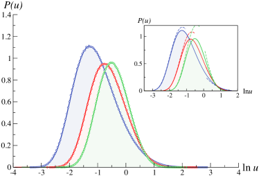
This behavior is, of course, consistent with the series expansions in Eqs.  (19), (20) and (21). Our results on the distribution $P(u)$ are summarized in Fig. 1.

Figure 2: (Color online) Distribution $P(\omega)$ for standard BM obtained from Eqs.  (23) and (29). $P(\omega=1/2)$ increases with the dimension $d$. The blue (lower) solid line corresponds to $d=1$, the red (middle) line to $d=2$ and the green (upper) line to $d=3$. Open circles with the same color code (and relative positions) present the results of numerical simulations for the LS estimator $u_{\delta}$ defined in Eq. (7). Note that an apparent coincidence of the results for the distributions $P(\omega)$ for the ML estimator in 2D and that for the LS estimator $u_{\delta}$ in 3D is accidental. It just signifies that the former outperforms the latter.

IV The distribution of the random variable $\omega$

Suppose next that we have two different independent realizations of BM trajectories, ${\bf B}_{1}(t)$ and ${\bf B}_{2}(t)$ which we use to generate to independent random variables $u_{1}$ and $u_{2}$. A natural question arising about their suitability as estimators is how likely is it that they will have the same value? Of course the distributions and thus moments of these two random variables are the same, however a measure of their relative dispersion can be deduced by studying the distribution function $P(\omega)$ of the random variable $\omega$ carlos ; carlos1 , defined in Eq. (3). This distribution is given explicitly by gleb

$$P(\omega)=\frac{1}{(1-\omega)^{2}}\int^{\infty}_{0}u\,du\,P(u)\,P\left(\frac{\omega}{1-\omega}u\right)$$ (29)

and hence, it suffices to know $P(u)$ in order to determine $P(\omega)$.

For $d=2$, (and, in fact, for any other even $d$), $P(\omega)$ can be evaluated exactly. Plugging Eq. (19) into (29), we get:

$$P(\omega)=4\sum_{k,l=1}^{\infty}\frac{\gamma_{k}}{J_{1}(\gamma_{k})}\frac{\gamma_{l}}{J_{1}(\gamma_{l})}\frac{1}{\left((1-\omega)\gamma_{k}^{2}+\omega\gamma_{l}^{2}\right)^{2}}$$ (30)

Performing the sum over $l$, we arrive at the following result for the distribution $P(\omega)$ in 2D systems

$$P(\omega)=2\frac{{\rm d}}{{\rm d}\omega}\sum_{k=1}^{\infty}\frac{1}{\gamma_{k}J_{1}(\gamma_{k})I_{0}(\gamma_{k}\sqrt{(1-\omega)/\omega})}\,.$$ (31)

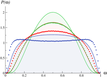
Numerically obtained distributions $P(\omega)$ for $d=1,2$ and $d=3$ dimensional systems are presented in Fig. 2. Notice that in all dimensions $\omega=1/2$ is the most probable value of the distribution $P(\omega)$ so that most probably $u_{1}=u_{2}$. Nevertheless, the distributions are rather broad which signifies that sample-to-sample fluctuations are rather important.

V Comparison of the LS and ML estimators.

We will now show that the ML estimator defined in Eq. (1) substantially outperforms the MS estimator as defined in Eq. (7) in any spatial dimension $d$. This is a very surprising result as one would intuitively expect, and it is often stated in the literature, that using the process $\delta_{T}$ has the effect of a reducing the fluctuations of the estimate of $D$ because the process is partially averaged in time.

To demonstrate this, we present in Fig. 3 a comparison of the analytical results for $P(u)$ of the ML estimator with the corresponding distributions of the LS estimator for $u_{\delta}$ obtained numerically.

Figure 3: (Color online) Comparison of $P(u)$ in Eq. (23) (solid lines) and the results of the numerical simulations for the distribution $P(u_{\delta})$ (histograms). From left to right: $d=1$, 2 and 3.

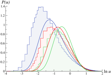
Indeed, we find that the variance of the distribution $P(u_{\delta})$ equals $1.38$, $0.66$ and $0.44$ for $d=1,2$ and $3$, respectively. The distribution of the ML estimator appears to be substantially narrower so that the variance is significantly lower, $1$, $1/2$ and $1/3$. Moreover, the most probable values of $u$ are closer to the ensemble average value $\mathbb{E}\{u\}\equiv 1$ than the most probable values of $P(u_{\delta})$ to $\mathbb{E}\{u_{\delta}\}\equiv 1$: we observe that the distribution $P(u_{\delta})$ attains its maximal values at $u_{\delta}\approx 0.15$, $0.33$ and $0.47$ for $d=1,2$ and $3$, respectively, while the corresponding maxima of the distribution $P(u)$ are located at $u\approx 0.28,0.47$ and $0.6$. Last but not least, the distribution $P(\omega_{\delta})$ appears to be significantly broader than $P(\omega)$, as revealed by Fig. 2. The worst performance of the LS estimator $u_{\delta}$ is in 1D systems in which the distribution $P(\omega_{\delta})$ has a bimodal $M$-shape with a local minimum at $\omega_{\delta}=1/2$, and maxima (most likely values) around $0.1$ and $0.9$. This means that the values $u_{1}$ and $u_{2}$ drawn from two different trajectories will most probably be different by an order of magnitude!

VI 1D Brownian motion in presence of disorder.

In this final section we address the question of how the distribution $P(u)$ of the ML estimator of a single trajectory diffusion coefficient will change in presence of quenched disorder. We will consider two different models of BM in random 1D environments - diffusion in presence of a random correlated potential and diffusion in presence of a random force.

Figure 4: (Color online) Distribution $P(u)$ for a particle diffusing in a random energy landscape with variance $\sigma^{2}$, correlation length $\xi_{c}=20$ and various disorder strengths $\epsilon=\beta\sigma$. From right to left: blue histogram corresponds to $\epsilon=0.5$, red - to $\epsilon=0.8$, green - to $\epsilon=1$, yellow - to $\epsilon=2$ and brown - to $\epsilon=3$. The walk duration is $T=10^{5}$, $t_{0}=0$ and averages are taken over $12,000$ walks occurring in independent landscapes. For comparison we present the distribution (solid black curve) for standard 1D BM ($\varepsilon\equiv 0$). The corresponding distributions $P(\omega)$ are shown in the inset ($P(\omega=1/2)$ decreases with increasing $\epsilon$).

VI.1 Diffusion in presence of a random potential

First we consider a BM in a 1D inhomogeneous energy landscape, where disorder is correlated over a finite length $\xi_{c}$. This model gives a simple description of diffusion of a protein along a DNA sequence, for instance, where the particle interacts with several neighboring base pairs at a time slutsky . The total binding energy of the protein is assumed to be a random variable. When the particle hops one neighboring base further to the right or to the left, its new energy is highly correlated to the value it had before the jump. Slutsky et al. slutsky modeled this process as a point-like particle diffusing on a 1D lattice of unit spacing with random site energies $\{U_{i}\}$, whose distribution is Gaussian with zero mean, variance $\sigma^{2}$ and is correlated in space as $\langle(U_{i}-U_{j})^{2}\rangle=2\sigma^{2}[1-\exp(-|i-j|/\xi_{c})]$. At each time step, the particle located at some site $i$ jumps to the left or to the right with probabilities $p_{i}\propto\exp[\beta(U_{i}-U_{i-1})]$ and $q_{i}\propto\exp[\beta(U_{i}-U_{i+1})]$, respectively, where $p_{i}+q_{i}=1$. Diffusion is asymptotically normal for any disorder strength $\epsilon=\beta\sigma$. Nevertheless, the particle can be trapped in local energy minima for long periods of time. During an extended intermediate time regime, it is observed that first passage properties fluctuate widely from one sample to another slutsky .

Our numerical simulations reveal that disorder has a dramatic effect on the distributions $P(u)$ and $P(\omega)$. As shown by Fig. 4, the distribution $P(u)$ broadens significantly in the small $u$ regime: very small values of the time-average diffusion constant (compared to the thermal and disorder average) become increasingly more probable as the disorder strength increases. However, the right tail of $P(u)$ is much less affected. Similarly, two independent measurements are likely to differ significantly, even in moderately disordered media (see inset of Fig. 4). When $\epsilon\approx 0.8$, the distribution $P(\omega)$ undergoes a continuous shape reversal transition - from a unimodal bell-shaped form to a bimodal $M$-shape one with the minimum at $\omega=1/2$ and two maxima approaching $0$ and $1$ at larger disorder strengths. Unfortunately, it does not seem possible to obtain this critical value analytically. Even for the case of a pure Brownian motion considered in Ref. carlos , such an analysis appears to be extremely difficult.

Therefore, for $\epsilon>0.8$ sample-to-sample fluctuations becomes essential and it is most likely that the diffusion coefficients drawn from two different trajectories will be different.

Figure 5: (Color online) In panel (a), distribution $P(u)$ for Sinai diffusion and different strengths of the disorder $\epsilon$. From right to left: blue histogram corresponds to $\epsilon=0.05$, red - to $\epsilon=0.1$, green - to $\epsilon=0.2$ and yellow - to $\epsilon=0.3$. The solid black curve depicts the distribution $P(u)$ for 1D BM ($\epsilon\equiv 0$), and the corresponding distributions $P(\omega)$ are shown in the inset with the same color code (for $\omega$ close to 0 or 1, $P(\omega)$ increases with $\epsilon$). In panel (b), distribution $P(\omega)$ for Sinai diffusion with $\epsilon=0.1$, the integration time is set to $T=10^{2}$ and $t_{0}$ is varied. $P(\omega=1/2)$ decreases with increasing $t_{0}$: the different curves corresponds to (from darker gray to lighter gray): $t_{0}=5$ (blue), $t_{0}=5\times 10^{2}$ (red), $t_{0}=5\times 10^{3}$ (green) and $t_{0}=5\times 10^{5}$ (yellow). In panel (c), the lag time is set to $t_{0}=5$ and the integration time $T$ is varied. $P(\omega=1/2)$ decreases with increasing $T$: $10^{2}$ (blue), $5\times 10^{4}$ (red), $1,5\times 10^{5}$ (green) and $2,5\times 10^{5}$ (yellow).

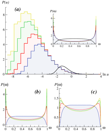
VI.2 Diffusion in presence of a random force

We discuss now the effect of disorder on the distributions $P(u)$ and $P(\omega)$ for 1D BM in presence of a quenched uncorrelated random force - the so-called Sinai diffusion Sinai1982 . In this model, one considers a random walk on a 1D infinite lattice and site $i$ dependent hopping probabilities: $p_{i}=\frac{1}{2}-\varepsilon_{i}$ for hopping from $i$ to the site $i+1$ and $q_{i}=\frac{1}{2}+\varepsilon_{i}$ for hopping to the site $i-1$. Here, $\varepsilon_{i}$ are independent, uncorrelated, identically distributed random variables with distribution $P(\varepsilon_{i})=\frac{1}{2}\delta(\varepsilon_{i}-\varepsilon)+\frac{1}{2}\delta(\varepsilon_{i}+\varepsilon)$ and the strength of disorder $\varepsilon$ is bounded away from $0$ and $1$. It is well-known that in the large-$t$ limit the model produces an anomalously slow sub-diffusion $\langle x^{2}(t)\rangle\sim\ln^{4}(t)$, where the angle brackets denote averaging with respect to different realizations of disorder. At shorter times, however, one observes an extended stage with a transient behavior which is substantially different from the asymptotic one. As a consequence, the statistics of $u$, defined in equation (1), and $\omega$ will depend not only on the integration time $T$ but also on the lag time $t_{0}$ from which a single trajectory is analyzed.

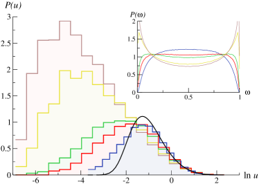
We have numerically computed the distributions $P(u)$ and $P(\omega)$. In Fig. 5$a$ we present the dependence of the $u$ and $\omega$ statistics on the strength of the disorder $\varepsilon$. As in the previous disordered potential case, we find that the maximum of $P(u)$ shifts toward zero as the disorder gets stronger. For comparison, the solid black line in Fig. 5$a$ represents $P(u)$ observed for standard BM, $\varepsilon\equiv 0$. Moreover, the stronger the disorder is, the broader the distribution $P(u)$ becomes, yielding more peaked maxima in $P(\omega)$ (see the inset of Fig. 5$a$). We also note that $P(\omega)$ has a bimodal $M$-shaped form even for the weakest disorder $\varepsilon=0.005$ that we have considered, suggesting that the zero-disorder limit is non-analytic compared to the continuous transition observed for diffusion in the random energy landscape of the previous section.

In Fig. 5$b$ and Fig. 5$c$, we show the statistics of $\omega$ for different values of $t_{0}$ and $T$. Increasing $t_{0}$ (or $T$) we observe that $P(\omega)$ changes from an almost uniform form, for which any relation between $u_{1}$ and $u_{2}$ is equally probable, to a bimodal $M$-shaped distribution, which signifies that in this regime two ML estimates $u_{1}$ and $u_{2}$ will most likely have different values. Bimodality is a property of the Sinai regime carlos , as also noticed earlier in Ref. redner , and thus it shows up only at sufficiently long times when the trajectories follow the asymptotic ultra-slow diffusion. The distribution $P(\omega)$ is remarkably sensitive to the characteristic aging of Sinai diffusion.

As a final observation, one may also study the statistics of $u$ for trajectories evolving in the same random force field. In this case (not shown here) one gets a narrow distribution for of $u$ and a unimodal $P(\omega)$ that converges to a delta singularity at $\omega=1/2$ when the disorder becomes infinite. This is due to the fact, known as Golosov phenomenon, that two trajectories in the same disorder will move together Golosov1983 .

VII Discussion

We have analyzed the reliability of the ML estimator for the diffusion constant of standard Brownian motion and shown its superiority over the more commonly used LS estimator in a number of important aspects, notably the variance of the estimator, the proximity of the most probable value to the true mean value and the distribution of the random variable $\omega$ which is a measure of the extent to which two estimations of $D$ vary. Going beyond the important test case of pure Brownian motion we have also analyzed the effect of quenched disorder, modeling fluctuations of the local energy landscape and forces. As one may have intuitively expected, the presence of short range disorder tends to broaden the distribution of the so measured value of $D$, as it presents an additional source of fluctuation. However in the Sinai model, in the same realization of the force field, trajectories are disorder dominated and are almost independent of the thermal noise, leading to highly peaked distributions of $D$. Analytically understanding the distribution of $D$ in the presence of disorder presents an interesting mathematical challenge which will involve analysis of the corresponding Schrödinger equation with a random drift term. Further interesting questions remain to be addressed, in particular can one use the two time correlation function of measured trajectories to obtain better estimators ? Single particle tracking technology will undoubtedly further improve in the coming years and many interesting mathematical, statistical and physical challenges will arise in the ultimate goal of getting the most out of the trajectories so obtained.