11institutetext: A. Kyrillidis 22institutetext: Laboratory for Information and Inference Systems, Ecole Polytechnique Federale de Lausanne
Tel.: +41 21 69 31154
22email: anastasios.kyrillidis@epfl.ch
33institutetext: V. Cevher 44institutetext: Laboratory for Information and Inference Systems, Ecole Polytechnique Federale de Lausanne
Tel.: +41 21 69 31101
44email: volkan.cevher@epfl.ch

Matrix Recipes for
Hard Thresholding Methods

\IEEEauthorblockNAnastasios Kyrillidis and Volkan Cevher
   Anastasios Kyrillidis    Volkan Cevher
(Received: date / Accepted: date)
Abstract

In this paper, we present and analyze a new set of low-rank recovery algorithms for linear inverse problems within the class of hard thresholding methods. We provide strategies on how to set up these algorithms via basic ingredients for different configurations to achieve complexity vs. accuracy tradeoffs. Moreover, we study acceleration schemes via memory-based techniques and randomized, ϵitalic-ϵ\epsilon-approximate matrix projections to decrease the computational costs in the recovery process. For most of the configurations, we present theoretical analysis that guarantees convergence under mild problem conditions. Simulation results demonstrate notable performance improvements as compared to state-of-the-art algorithms both in terms of reconstruction accuracy and computational complexity.

Keywords:
Affine rank minimization hard thresholding ϵitalic-ϵ\epsilon-approximation schemes randomized algorithms.

1 Introduction

In this work, we consider the general affine rank minimization (ARM) problem, described as follows: The ARM Problem: Assume 𝐗m×nsuperscript𝐗superscript𝑚𝑛\boldsymbol{X}^{\ast}\in\mathbb{R}^{m\times n} is a rank-k𝑘k matrix of interest (kmin{m,n}much-less-than𝑘𝑚𝑛k\ll\min\{m,n\}) and let 𝓐:m×np:𝓐superscript𝑚𝑛superscript𝑝\boldsymbol{\mathcal{A}}:\mathbb{R}^{m\times n}\rightarrow\mathbb{R}^{p} be a known linear operator. Given a set of observations as 𝐲=𝓐𝐗+𝛆p𝐲𝓐superscript𝐗𝛆superscript𝑝\boldsymbol{y}=\boldsymbol{\mathcal{A}}\boldsymbol{X}^{\ast}+\boldsymbol{\varepsilon}\in\mathbb{R}^{p}, we desire to recover 𝐗superscript𝐗\boldsymbol{X}^{\ast}from 𝐲𝐲\boldsymbol{y} in a scalable and robust manner. The challenge in this problem is to recover the true low-rank matrix in subsampled settings where pmnmuch-less-than𝑝𝑚𝑛p\ll m\cdot n. In such cases, we typically exploit the prior information that 𝑿superscript𝑿\boldsymbol{X}^{\ast} is low-rank and thus, we are interested in finding a matrix 𝑿𝑿\boldsymbol{X} of rank at most k𝑘k that minimizes the data error f(𝑿):=𝒚𝓐𝑿22assign𝑓𝑿superscriptsubscriptnorm𝒚𝓐𝑿22f(\boldsymbol{X}):=\|\boldsymbol{y}-\boldsymbol{\mathcal{A}}\boldsymbol{X}\|_{2}^{2} as follows:

minimize𝑿m×n𝑿superscript𝑚𝑛minimize\displaystyle\underset{\boldsymbol{X}\in\mathbb{R}^{m\times n}}{\text{minimize}} f(𝑿)𝑓𝑿\displaystyle f(\boldsymbol{X}) (1)
subject to rank(𝑿)k.rank𝑿𝑘\displaystyle\text{rank}(\boldsymbol{X})\leq k.

The ARM problem appears in many applications; low dimensional embedding baraniuk2010low , matrix completion candès2009exact , image compression SVP , function learning TyagiCevherRidge ; TyagiCevherRidgeII just to name a few. We present below important ARM problem cases, as characterized by the nature of the linear operator 𝓐𝓐\boldsymbol{\mathcal{A}}.

General linear maps: In many ARM problem cases, 𝓐𝓐\boldsymbol{\mathcal{A}} or 𝓐superscript𝓐\boldsymbol{\mathcal{A}}^{\ast} has a dense range, satisfying specific incoherence or restricted isometry properties (discussed later in the paper); here, 𝓐superscript𝓐\boldsymbol{\mathcal{A}}^{\ast} is the adjoint operator of 𝓐𝓐\boldsymbol{\mathcal{A}}. In Quantum Tomography, liuuniversal studies the Pauli operator, a compressive linear map 𝓐𝓐\boldsymbol{\mathcal{A}} that consists of the kronecker product of 2×2222\times 2 matrices and obeys restricted isometry properties, defined later in the paper. Furthermore, recent developments indicate connections of ridge function learning TyagiCevherRidge ; hemant2012active and phase retrieval candes2012solving with the ARM problem where 𝓐𝓐\boldsymbol{\mathcal{A}} is a Bernoulli and a Fourier operator, respectively.

Matrix Completion (MC): Let ΩΩ\Omega be the set of ordered pairs that represent the coordinates of the observable entries in 𝑿superscript𝑿\boldsymbol{X}^{\ast}. Then, the set of observations satisfy 𝒚=𝓐Ω𝑿+𝜺𝒚subscript𝓐Ωsuperscript𝑿𝜺\boldsymbol{y}=\boldsymbol{\mathcal{A}}_{\Omega}\boldsymbol{X}^{\ast}+\boldsymbol{\varepsilon} where 𝓐Ωsubscript𝓐Ω\boldsymbol{\mathcal{A}}_{\Omega} defines a linear mask over the observable entries ΩΩ\Omega. To solve the MC problem, a potential criterion is given by (1) candès2009exact . As a motivating example, consider the famous Netflix problem netflix , a recommender system problem where users’ movie preferences are inferred by a limited subset of entries in a database.

Principal Component Analysis: In Principal Component Analysis (PCA), we are interested in identifying a low rank subspace that best explains the data in the Euclidean sense from the observations 𝒚=𝓐𝑿𝒚𝓐superscript𝑿\boldsymbol{y}=\boldsymbol{\mathcal{A}}\boldsymbol{X}^{\ast} where 𝓐:m×np:𝓐superscript𝑚𝑛superscript𝑝\boldsymbol{\mathcal{A}}:\mathbb{R}^{m\times n}\rightarrow\mathbb{R}^{p} is an identity linear map that stacks the columns of the matrix 𝑿superscript𝑿\boldsymbol{X}^{\ast} into a single column vector with p=mn𝑝𝑚𝑛p=m\cdot n. We observe that the PCA problem falls under the ARM criterion in (1). While (1) is generally NP-hard to solve optimally, PCA can be solved in polynomial time using the truncated Singular Value Decomposition (SVD) of 𝓐𝒚superscript𝓐𝒚\boldsymbol{\mathcal{A}}^{\ast}\boldsymbol{y}. As an extension to the PCA setting, candes2011robust considers the Robust PCA problem where 𝒚𝒚\boldsymbol{y} is further corrupted by gross sparse noise. We extend the framework proposed in this paper for the RPCA case and its generalizations in KyrillidisCevherSSP .

For the rest of the paper, we consider only the low rank estimation case in (1). As running test cases to support our claims, we consider the MC setting as well as the general ARM setting where 𝓐𝓐\boldsymbol{\mathcal{A}} is constituted by permuted subsampled noiselets sparcs .

1.1 Two camps of recovery algorithms

Convex relaxations: In brecht2010 , the authors study the nuclear norm 𝑿subscriptnorm𝑿\|\boldsymbol{X}\|_{\ast} :=i=1rank(𝑿)σiassignabsentsuperscriptsubscript𝑖1rank𝑿subscript𝜎𝑖:=\sum_{i=1}^{\text{rank}(\boldsymbol{X})}\sigma_{i} as a convex surrogate of rank(𝑿)rank𝑿\text{rank}(\boldsymbol{X}) operator so that we can leverage convex optimization approaches, such as interior-point methods—here, σisubscript𝜎𝑖\sigma_{i} denotes the i𝑖i-th singular value of 𝑿𝑿\boldsymbol{X}. Under basic incoherence properties of the sensing linear mapping 𝓐𝓐\boldsymbol{\mathcal{A}}, brecht2010 provides provable guarantees for unique low rank matrix recovery using the nuclear norm.

Once (1) is relaxed to a convex problem, decades of knowledge on convex analysis and optimization can be leveraged. Interior point methods find a solution with fixed precision in polynomial time but their complexity might be prohibitive even for moderate-sized problems Liu2009 ; Fazel2010 . More suitable for large-scale data analysis, first-order methods constitute low-complexity alternatives but most of them introduce complexity vs. accuracy tradeoffs SVT ; ParallelRecht ; ALM ; APG .

Non-convex approaches: In contrast to the convex relaxation approaches, iterative greedy algorithms maintain the nonconvex nature of (1). Unfortunately, solving (1) optimally is in general NP-hard natarajan1995sparse . Due to this computational intractability, the algorithms in this class greedily refine a rank-k𝑘k solution using only “local” information available at the current iteration admira2010 ; Goldfarb:2011 ; beck2011linearly .

1.2 Contributions

In this work, we study a special class of iterative greedy algorithms known as hard thresholding methods. Similar results have been derived for the vector case KyrillidisCevherRecipes . Note that the transition from sparse vector approximation to ARM is non-trivial; while s𝑠s-sparse signals “live” in the union of finite number of subspaces, the set of rank-k𝑘k matrices expands to infinitely many subspaces. Thus, the selection rules do not generalize in a straightforward way.

Our contributions are the following:

Ingredients of hard thresholding methods: We analyze the behaviour and performance of hard thresholding methods from a global perspective. Five building blocks are studied: i)i) step size selection μisubscript𝜇𝑖\mu_{i}, ii)ii) gradient or least-squares updates over restricted low-rank subspaces (e.g., adaptive block coordinate descent), iii)iii) memory exploitation, iv)iv) active low-rank subspace tracking and, v)v) low-rank matrix approximations (described next). We highlight the impact of these key pieces on the convergence rate and signal reconstruction performance and provide optimal and/or efficient strategies on how to set up these ingredients under different problem conditions.

Low-rank matrix approximations in hard thresholding methods: In clash , the authors show that the solution efficiency can be significantly improved by ϵitalic-ϵ\epsilon-approximation algorithms. Based on similar ideas, we analyze the impact of ϵitalic-ϵ\epsilon-approximate low rank-revealing schemes in the proposed algorithms with well-characterized time and space co- mplexities. Moreover, we provide extensive analysis to prove convergence using ϵitalic-ϵ\epsilon-approximate low-rank projections.

Hard thresholding-based framework with improved convergence conditions: We study hard thresholding variants that provide salient computational tradeoffs for the class of greedy methods on low-rank matrix recovery. These methods, as they iterate, exploit the non-convex scaffold of low rank subspaces on which the approximation problem resides. Using simple analysis tools, we derive improved conditions that guarantee convergence, compared to state-of-the-art approaches.

The organization of the paper is as follows. In Section 2, we set up the notation and provide some definitions and properties, essential for the rest of the paper. In Section 3, we describe the basic algorithmic frameworks in a nutshell, while in Section 4 we provide important “ingredients” for the class of hard-thresholding methods; detailed convergence analysis proofs are provided in Section 5. The complexity analysis of the proposed algorithms is provided in Section 6. We study two acceleration schemes in Sections 7 and 8, based on memory utilization and ϵitalic-ϵ\epsilon-approximate low-rank projections, respectively. We further improve convergence speed by exploiting randomized low rank projections in Section 9, based on power iteration-based subspace finder tools findingstructure . We provide empirical support for our claims through experimental results on synthetic and real data in Section 10. Finally, we conclude with future work directions in Section 11.

2 Elementary Definitions and Properties

We reserve lower-case and bold lower-case letters for scalar and vector variable representation, respectively. Bold upper-case letters denote matrices while bold calligraphic upper-case letters represent linear operators. We use calligraphic upper-case letters for set representations. We use 𝑿(i)𝑿𝑖\boldsymbol{X}(i) to represent the matrix estimate at the i𝑖i-th iteration.

The rank of 𝑿𝑿\boldsymbol{X} is denoted as rank(𝑿)min{m,n}rank𝑿𝑚𝑛\text{rank}(\boldsymbol{X})\leq\min\{m,n\}. The empirical data error is denoted as f(𝑿):=𝒚𝓐𝑿22assign𝑓𝑿superscriptsubscriptnorm𝒚𝓐𝑿22f(\boldsymbol{X}):=\|\boldsymbol{y}-\boldsymbol{\mathcal{A}}\boldsymbol{X}\|_{2}^{2} with gradient f(𝑿):=2𝓐(𝒚𝓐𝑿)assign𝑓𝑿2superscript𝓐𝒚𝓐𝑿\nabla f(\boldsymbol{X}):=-2\boldsymbol{\mathcal{A}}^{\ast}(\boldsymbol{y}-\boldsymbol{\mathcal{A}}\boldsymbol{X}), where is the adjoint operation over the linear mapping 𝓐𝓐\boldsymbol{\mathcal{A}}. The inner product between matrices 𝑨,𝑩m×n𝑨𝑩superscript𝑚𝑛\boldsymbol{A},~{}\boldsymbol{B}\in\mathbb{R}^{m\times n} is denoted as 𝑨,𝑩=trace(𝑩T𝑨)𝑨𝑩tracesuperscript𝑩𝑇𝑨\left\langle\boldsymbol{A},\boldsymbol{B}\right\rangle=\text{trace}(\boldsymbol{B}^{T}\boldsymbol{A}), where T represents the transpose operation. 𝐈𝐈\mathbf{I} represents an identity matrix with dimensions apparent from the context.

Let 𝒮𝒮\mathcal{S} be a set of orthonormal, rank-1 matrices that span an arbitrary subspace in m×nsuperscript𝑚𝑛\mathbb{R}^{m\times n}. We reserve span(𝒮)span𝒮\text{span}(\mathcal{S}) to denote the subspace spanned by 𝒮𝒮\mathcal{S}. With slight abuse of notation, we use:

rank(span(𝒮))max𝑿{rank(𝑿):𝑿span(𝒮)},rankspan𝒮subscript𝑿:rank𝑿𝑿span𝒮\displaystyle\text{rank}(\text{span}(\mathcal{S}))\equiv\max_{\boldsymbol{X}}\left\{\text{rank}(\boldsymbol{X}):~{}\boldsymbol{X}\in\text{span}(\mathcal{S})\right\}, (2)

to denote the maximum rank a matrix 𝑿m×n𝑿superscript𝑚𝑛\boldsymbol{X}\in\mathbb{R}^{m\times n} can have such that 𝑿𝑿\boldsymbol{X} lies in the subspace spanned by the set 𝒮𝒮\mathcal{S}. Given a finite set 𝒮𝒮\mathcal{S}, |𝒮|𝒮|\mathcal{S}| denotes the cardinality of 𝒮𝒮\mathcal{S}. For any matrix 𝑿𝑿\boldsymbol{X}, we use R(𝑿)𝑅𝑿R(\boldsymbol{X}) to denote its range.

We define a minimum cardinality set of orthonormal, rank-1 matrices that span the subspace induced by a set of rank-1 (and possibly non-orthogonal) matrices 𝒮𝒮\mathcal{S} as:

ortho(𝒮)argmin𝒯{|𝒯|:𝒯𝒰s.t.span(𝒯)=span(𝒮)},ortho𝒮subscriptargmin𝒯:𝒯𝒯𝒰s.t.span𝒯span𝒮\displaystyle\text{ortho}(\mathcal{S})\in\operatorname*{arg\,min}_{\mathcal{T}}\{|\mathcal{T}|:\mathcal{T}\subseteq\mathcal{U}~{}\text{s.t.}~{}\text{span}(\mathcal{T})=\text{span}(\mathcal{S})\},

where 𝒰𝒰\mathcal{U} denotes the superset that includes all the sets of orthonormal, rank-1 matrices in m×nsuperscript𝑚𝑛\mathbb{R}^{m\times n} such that 𝑻i,𝑻j=0,ij,formulae-sequencesubscript𝑻𝑖subscript𝑻𝑗0𝑖𝑗\langle\boldsymbol{T}_{i},\boldsymbol{T}_{j}\rangle=0,~{}i\neq j, 𝑻i,𝑻j𝒯for-allsubscript𝑻𝑖subscript𝑻𝑗𝒯\forall\boldsymbol{T}_{i},\boldsymbol{T}_{j}\in\mathcal{T} and, 𝑻iF=1,isubscriptnormsubscript𝑻𝑖𝐹1for-all𝑖\big{\|}\boldsymbol{T}_{i}\big{\|}_{F}=1,~{}\forall i. In general, ortho(𝒮)ortho𝒮\text{ortho}(\mathcal{S}) is not unique.

A well-known lemma used in the convergence rate proofs of this class of greedy hard thresholding algorithms is defined next.

Lemma 1

Bertsekas Let 𝒥m×n𝒥superscript𝑚𝑛\mathcal{J}\subseteq\mathbb{R}^{m\times n} be a closed convex set and f:𝒥:𝑓𝒥f:\mathcal{J}\rightarrow\mathbb{R} be a smooth objective function defined over 𝒥𝒥\mathcal{J}. Let 𝐗𝒥superscript𝐗𝒥\boldsymbol{X}^{\ast}\in\mathcal{J} be a local minimum of the objective function f𝑓f over the set 𝒥𝒥\mathcal{J}. Then

f(𝑿),𝑿𝑿0,𝑿𝒥.formulae-sequence𝑓superscript𝑿𝑿superscript𝑿0for-all𝑿𝒥\displaystyle\langle\nabla f(\boldsymbol{X}^{\ast}),\boldsymbol{X}-\boldsymbol{X}^{\ast}\rangle\geq 0,\;\;\forall\boldsymbol{X}\in\mathcal{J}. (3)

2.1 Singular Value Decomposition (SVD) and its properties

Definition 1

[SVD] Let 𝑿m×n𝑿superscript𝑚𝑛\boldsymbol{X}\in\mathbb{R}^{m\times n} be a rank-l𝑙l (l<min𝑙l<\min {m,n}𝑚𝑛\{m,n\}) matrix. Then, the SVD of 𝑿𝑿\boldsymbol{X} is given by:

𝑿=𝑼𝚺𝑽T=[𝑼α𝑼β][𝚺~𝟎𝟎𝟎][𝑽αT𝑽βT],𝑿𝑼𝚺superscript𝑽𝑇matrixsubscript𝑼𝛼subscript𝑼𝛽matrix~𝚺000matrixsuperscriptsubscript𝑽𝛼𝑇superscriptsubscript𝑽𝛽𝑇\displaystyle\boldsymbol{X}=\boldsymbol{U}\boldsymbol{\Sigma}\boldsymbol{V}^{T}=\begin{bmatrix}\boldsymbol{U}_{\alpha}&\boldsymbol{U}_{\beta}\end{bmatrix}\begin{bmatrix}\widetilde{\boldsymbol{\Sigma}}&\boldsymbol{0}\\ \boldsymbol{0}&\boldsymbol{0}\end{bmatrix}\begin{bmatrix}\boldsymbol{V}_{\alpha}^{T}\\ \boldsymbol{V}_{\beta}^{T}\end{bmatrix}, (4)

where 𝑼αm×l,𝑼βm×(ml),𝑽αn×l,𝑽βn×(nl)formulae-sequencesubscript𝑼𝛼superscript𝑚𝑙formulae-sequencesubscript𝑼𝛽superscript𝑚𝑚𝑙formulae-sequencesubscript𝑽𝛼superscript𝑛𝑙subscript𝑽𝛽superscript𝑛𝑛𝑙\boldsymbol{U}_{\alpha}\in\mathbb{R}^{m\times l},\boldsymbol{U}_{\beta}\in\mathbb{R}^{m\times(m-l)},\boldsymbol{V}_{\alpha}\in\mathbb{R}^{n\times l},\boldsymbol{V}_{\beta}\in\mathbb{R}^{n\times(n-l)} and 𝚺~=diag(σ1,,σl)l×l~𝚺diagsubscript𝜎1subscript𝜎𝑙superscript𝑙𝑙\widetilde{\boldsymbol{\Sigma}}=\text{diag}(\sigma_{1},\dots,\sigma_{l})\in\mathbb{R}^{l\times l} for σ1,,subscript𝜎1\sigma_{1},\dots, σl+subscript𝜎𝑙subscript\sigma_{l}\in\mathbb{R}_{+}. Here, the columns of 𝑼,𝑽𝑼𝑽\boldsymbol{U},\boldsymbol{V} represent the set of left and right singular vectors, respectively, and σ1,,σlsubscript𝜎1subscript𝜎𝑙\sigma_{1},\dots,\sigma_{l} denote the singular values.

For any matrix 𝑿m×n𝑿superscript𝑚𝑛\boldsymbol{X}\in\mathbb{R}^{m\times n} with arbitrary rank(𝑿)min{m,n}rank𝑿𝑚𝑛\text{rank}(\boldsymbol{X})\leq\min\{m,n\}, its best orthogonal projection 𝒫k(𝑿)subscript𝒫𝑘𝑿\mathcal{P}_{k}(\boldsymbol{X}) onto the set of rank-k𝑘k (k<rank(𝑿)𝑘rank𝑿k<\text{rank}(\boldsymbol{X})) matrices 𝒞k:={𝑨m×n:rank(𝑨)k}assignsubscript𝒞𝑘conditional-set𝑨superscript𝑚𝑛rank𝑨𝑘\mathcal{C}_{k}:=\{\boldsymbol{A}\in\mathbb{R}^{m\times n}:\text{rank}(\boldsymbol{A})\leq k\} defines the optimization problem:

𝒫k(𝑿)argmin𝒀𝒞k𝒀𝑿F.subscript𝒫𝑘𝑿subscriptargmin𝒀subscript𝒞𝑘subscriptnorm𝒀𝑿𝐹\displaystyle\mathcal{P}_{k}(\boldsymbol{X})\in\operatorname*{arg\,min}_{\boldsymbol{Y}\in\mathcal{C}_{k}}\big{\|}\boldsymbol{Y}-\boldsymbol{X}\big{\|}_{F}. (5)

According to the Eckart-Young theorem horn1990matrix , the best rank-k𝑘k approximation of a matrix 𝑿𝑿\boldsymbol{X} corresponds to its truncated SVD: if 𝑿=𝑼𝚺𝑽T𝑿𝑼𝚺superscript𝑽𝑇\boldsymbol{X}=\boldsymbol{U}\boldsymbol{\Sigma}\boldsymbol{V}^{T}, then 𝒫k(𝑿):=𝑼k𝚺k𝑽kTassignsubscript𝒫𝑘𝑿subscript𝑼𝑘subscript𝚺𝑘superscriptsubscript𝑽𝑘𝑇\mathcal{P}_{k}(\boldsymbol{X}):=\boldsymbol{U}_{k}\boldsymbol{\Sigma}_{k}\boldsymbol{V}_{k}^{T} where 𝚺kk×ksubscript𝚺𝑘superscript𝑘𝑘\boldsymbol{\Sigma}_{k}\in\mathbb{R}^{k\times k} is a diagonal matrix that contains the first k𝑘k diagonal entries of 𝚺𝚺\boldsymbol{\Sigma} and 𝑼k,𝑽ksubscript𝑼𝑘subscript𝑽𝑘\boldsymbol{U}_{k},~{}\boldsymbol{V}_{k} contain the corresponding left and right singular vectors, respectively. Moreover, this projection is not always unique. In the case of multiple identical singular values, the lexicographic approach is used to break ties. In any case, 𝒫k(𝑿)𝑿F𝑾𝑿Fsubscriptnormsubscript𝒫𝑘𝑿𝑿𝐹subscriptnorm𝑾𝑿𝐹\big{\|}\mathcal{P}_{k}(\boldsymbol{X})-\boldsymbol{X}\big{\|}_{F}\leq\big{\|}\boldsymbol{W}-\boldsymbol{X}\big{\|}_{F} for any rank-k𝑘k 𝑾m×n𝑾superscript𝑚𝑛\boldsymbol{W}\in\mathbb{R}^{m\times n}.

2.2 Subspace projections

Given a set of orthonormal, rank-1 matrices 𝒮𝒮\mathcal{S}, we denote the orthogonal projection operator onto the subspace induced by 𝒮𝒮\mathcal{S} as 𝒫𝒮subscript𝒫𝒮\mathcal{P}_{\mathcal{S}}111The distinction between 𝒫𝒮subscript𝒫𝒮\mathcal{P}_{\mathcal{S}} and 𝒫ksubscript𝒫𝑘\mathcal{P}_{k} for k𝑘k positive integer is apparent from context. which is an idempotent linear transformation; furthermore, we denote the orthogonal projection operator onto the orthogonal subspace of 𝒮𝒮\mathcal{S} as 𝒫𝒮subscript𝒫superscript𝒮bottom\mathcal{P}_{\mathcal{S}^{\bot}}. We can always decompose a matrix 𝑿m×n𝑿superscript𝑚𝑛\boldsymbol{X}\in\mathbb{R}^{m\times n} into two matrix components, as follows:

𝑿:=𝒫𝒮𝑿+𝒫𝒮𝑿,such that𝒫𝒮𝑿,𝒫𝒮𝑿=0.formulae-sequenceassign𝑿subscript𝒫𝒮𝑿subscript𝒫superscript𝒮bottom𝑿such thatsubscript𝒫𝒮𝑿subscript𝒫superscript𝒮bottom𝑿0\displaystyle\boldsymbol{X}:=\mathcal{P}_{\mathcal{S}}\boldsymbol{X}+\mathcal{P}_{\mathcal{S}^{\bot}}\boldsymbol{X},~{}~{}\text{such that}~{}\langle\mathcal{P}_{\mathcal{S}}\boldsymbol{X},\mathcal{P}_{\mathcal{S}^{\bot}}\boldsymbol{X}\rangle=0.

If 𝑿span(𝒮)𝑿span𝒮\boldsymbol{X}\in\text{span}(\mathcal{S}), the best projection of 𝑿𝑿\boldsymbol{X} onto the subspace induced by 𝒮𝒮\mathcal{S} is the matrix 𝑿𝑿\boldsymbol{X} itself. Moreover, 𝒫𝒮𝑿F𝑿Fsubscriptnormsubscript𝒫𝒮𝑿𝐹subscriptnorm𝑿𝐹\big{\|}\mathcal{P}_{\mathcal{S}}\boldsymbol{X}\big{\|}_{F}\leq\big{\|}\boldsymbol{X}\big{\|}_{F} for any 𝒮𝒮\mathcal{S} and 𝑿𝑿\boldsymbol{X}.

Definition 2

[Orthogonal projections using SVD] Let 𝑿m×n𝑿superscript𝑚𝑛\boldsymbol{X}\in\mathbb{R}^{m\times n} be a matrix with arbitrary rank and SVD decomposition given by (4). Then, 𝒮:={𝒖i𝒗iT:i=1,,k}assign𝒮conditional-setsubscript𝒖𝑖superscriptsubscript𝒗𝑖𝑇𝑖1𝑘\mathcal{S}:=\{\boldsymbol{u}_{i}\boldsymbol{v}_{i}^{T}:i=1,\dots,k\} (krank(𝑿)𝑘rank𝑿k\leq\text{rank}(\boldsymbol{X})) constitutes a set of orthonormal, rank-1 matrices that spans the best k𝑘k-rank subspace in R(𝑿)𝑅𝑿R(\boldsymbol{X}) and R(𝑿T)𝑅superscript𝑿𝑇R(\boldsymbol{X}^{T}); here, 𝒖isubscript𝒖𝑖\boldsymbol{u}_{i} and 𝒗isubscript𝒗𝑖\boldsymbol{v}_{i} denote the i𝑖i-th left and right singular vectors, respectively. The orthogonal projection onto this subspace is given by candès2009exact :

𝒫𝒮𝑿=𝒫𝒰𝑿+𝑿𝒫𝒱𝒫𝒰𝑿𝒫𝒱subscript𝒫𝒮𝑿subscript𝒫𝒰𝑿𝑿subscript𝒫𝒱subscript𝒫𝒰𝑿subscript𝒫𝒱\displaystyle\mathcal{P}_{\mathcal{S}}\boldsymbol{X}=\mathcal{P}_{\mathcal{U}}\boldsymbol{X}+\boldsymbol{X}\mathcal{P}_{\mathcal{V}}-\mathcal{P}_{\mathcal{U}}\boldsymbol{X}\mathcal{P}_{\mathcal{V}} (6)

where 𝒫𝒰=𝑼:,1:k𝑼:,1:kTsubscript𝒫𝒰subscript𝑼::1𝑘superscriptsubscript𝑼::1𝑘𝑇\mathcal{P}_{\mathcal{U}}=\boldsymbol{U}_{:,1:k}\boldsymbol{U}_{:,1:k}^{T} and 𝒫𝒱=𝑽:,1:k𝑽:,1:kTsubscript𝒫𝒱subscript𝑽::1𝑘superscriptsubscript𝑽::1𝑘𝑇\mathcal{P}_{\mathcal{V}}=\boldsymbol{V}_{:,1:k}\boldsymbol{V}_{:,1:k}^{T} in Matlab notation. Moreover, the orthogonal projection onto the 𝒮superscript𝒮bottom\mathcal{S}^{\bot} is given by:

𝒫𝒮𝑿=𝑿𝒫𝒮𝑿.subscript𝒫superscript𝒮bottom𝑿𝑿subscript𝒫𝒮𝑿\displaystyle\mathcal{P}_{\mathcal{S}^{\bot}}\boldsymbol{X}=\boldsymbol{X}-\mathcal{P}_{\mathcal{S}}\boldsymbol{X}. (7)

In the algorithmic descriptions, we use 𝒮𝒫k(𝑿)𝒮subscript𝒫𝑘𝑿\mathcal{S}\leftarrow\mathcal{P}_{k}\left(\boldsymbol{X}\right) to denote the set of rank-1, orthonormal matrices as outer products of the k𝑘k left 𝒖isubscript𝒖𝑖\boldsymbol{u}_{i} and right 𝒗isubscript𝒗𝑖\boldsymbol{v}_{i} principal singular vectors of 𝑿𝑿\boldsymbol{X} that span the best rank-k𝑘k subspace of 𝑿𝑿\boldsymbol{X}; e.g. 𝒮={𝒖i𝒗i,i=1,,k}\mathcal{S}=\{\boldsymbol{u}_{i}\boldsymbol{v}_{i},~{}i=1,\dots,k\}. Moreover, 𝑿^𝒫k(𝑿)^𝑿subscript𝒫𝑘𝑿\widehat{\boldsymbol{X}}\leftarrow\mathcal{P}_{k}\left(\boldsymbol{X}\right) denotes a/the best rank-k𝑘k projection matrix of 𝑿𝑿\boldsymbol{X}. In some cases, we use {𝒮,𝑿^}𝒫k(𝑿)𝒮^𝑿subscript𝒫𝑘𝑿\{\mathcal{S},~{}\widehat{\boldsymbol{X}}\}\leftarrow\mathcal{P}_{k}\left(\boldsymbol{X}\right) when we compute both. The distiction between these cases is apparent from the context.

2.3 Restricted Isometry Property

Many conditions have been proposed in the literature to establish solution uniqueness and recovery stability such as null space property cohen06 , exact recovery condition Tro04:Greed-Good , etc. For the matrix case, brecht2010 proposed the restricted isometry property (RIP) for the ARM problem.

Definition 3

[Rank Restricted Isometry Property (R-RIP) for matrix linear operators brecht2010 ] A linear operator 𝓐:m×n:𝓐superscript𝑚𝑛\boldsymbol{\mathcal{A}}:\mathbb{R}^{m\times n} pabsentsuperscript𝑝\rightarrow\mathbb{R}^{p} satisfies the R-RIP with constant δk(𝓐)(0,1)subscript𝛿𝑘𝓐01\delta_{k}(\boldsymbol{\mathcal{A}})\in(0,1) if and only if:

(1δk(𝓐))𝑿F2𝓐𝑿22(1+δk(𝓐))𝑿F2,1subscript𝛿𝑘𝓐superscriptsubscriptnorm𝑿𝐹2superscriptsubscriptnorm𝓐𝑿221subscript𝛿𝑘𝓐superscriptsubscriptnorm𝑿𝐹2(1-\delta_{k}(\boldsymbol{\mathcal{A}}))\big{\|}\boldsymbol{X}\big{\|}_{F}^{2}\leq\big{\|}\boldsymbol{\mathcal{A}}\boldsymbol{X}\big{\|}_{2}^{2}\leq(1+\delta_{k}(\boldsymbol{\mathcal{A}}))\big{\|}\boldsymbol{X}\big{\|}_{F}^{2}, (8)

𝑿m×nsuch thatrank(𝑿)k.for-all𝑿superscript𝑚𝑛such thatrank𝑿𝑘~{}~{}\forall\boldsymbol{X}\in\mathbb{R}^{m\times n}~{}\text{such that}~{}\text{rank}(\boldsymbol{X})\leq k. We write δksubscript𝛿𝑘\delta_{k} to mean δk(𝓐)subscript𝛿𝑘𝓐\delta_{k}(\boldsymbol{\mathcal{A}}), unless otherwise stated.

liuuniversal shows that Pauli operators satisfy the rank-RIP in compressive settings while, in function learning, the linear map 𝓐𝓐\boldsymbol{\mathcal{A}} is designed specifically to satisfy the rank-RIP hemant2012active .

2.4 Some useful bounds using R-RIP

In this section, we present some lemmas that are useful in our subsequent developments—these lemmas are consequen- ces of the R-RIP of 𝓐𝓐\boldsymbol{\mathcal{A}}.

Lemma 2

admira2010 Let 𝓐:m×np:𝓐superscript𝑚𝑛superscript𝑝\boldsymbol{\mathcal{A}}:\mathbb{R}^{m\times n}\rightarrow\mathbb{R}^{p} be a linear operator that satisfies the R-RIP with constant δksubscript𝛿𝑘\delta_{k}. Then, 𝐯pfor-all𝐯superscript𝑝\forall\boldsymbol{v}\in\mathbb{R}^{p}, the following holds true:

𝒫𝒮(𝓐𝒗)F1+δk𝒗2,subscriptnormsubscript𝒫𝒮superscript𝓐𝒗𝐹1subscript𝛿𝑘subscriptnorm𝒗2\displaystyle\big{\|}\mathcal{P}_{\mathcal{S}}(\boldsymbol{\mathcal{A}}^{\ast}\boldsymbol{v})\big{\|}_{F}\leq\sqrt{1+\delta_{k}}\big{\|}\boldsymbol{v}\big{\|}_{2}, (9)

where 𝒮𝒮\mathcal{S} is a set of orthonormal, rank-1 matrices in m×nsuperscript𝑚𝑛\mathbb{R}^{m\times n} such that rank(𝒫𝒮𝐗)k,𝐗m×nformulae-sequenceranksubscript𝒫𝒮𝐗𝑘for-all𝐗superscript𝑚𝑛\text{rank}(\mathcal{P}_{\mathcal{S}}\boldsymbol{X})\leq k,~{}\forall\boldsymbol{X}\in\mathbb{R}^{m\times n}.

Lemma 3

admira2010 Let 𝓐:m×np:𝓐superscript𝑚𝑛superscript𝑝\boldsymbol{\mathcal{A}}:\mathbb{R}^{m\times n}\rightarrow\mathbb{R}^{p} be a linear operator that satisfies the R-RIP with constant δksubscript𝛿𝑘\delta_{k}. Then, 𝐗m×nfor-all𝐗superscript𝑚𝑛\forall\boldsymbol{X}\in\mathbb{R}^{m\times n}, the following holds true:

(1δk)𝒫𝒮𝑿F1subscript𝛿𝑘subscriptnormsubscript𝒫𝒮𝑿𝐹\displaystyle(1-\delta_{k})\big{\|}\mathcal{P}_{\mathcal{S}}\boldsymbol{X}\big{\|}_{F} 𝒫𝒮𝓐𝓐𝒫𝒮𝑿Fabsentsubscriptnormsubscript𝒫𝒮superscript𝓐𝓐subscript𝒫𝒮𝑿𝐹\displaystyle\leq\big{\|}\mathcal{P}_{\mathcal{S}}\boldsymbol{\mathcal{A}}^{\ast}\boldsymbol{\mathcal{A}}\mathcal{P}_{\mathcal{S}}\boldsymbol{X}\big{\|}_{F}
(1+δk)𝒫𝒮𝑿F,absent1subscript𝛿𝑘subscriptnormsubscript𝒫𝒮𝑿𝐹\displaystyle\leq(1+\delta_{k})\big{\|}\mathcal{P}_{\mathcal{S}}\boldsymbol{X}\big{\|}_{F}, (10)

where 𝒮𝒮\mathcal{S} is a set of orthonormal, rank-1 matrices in m×nsuperscript𝑚𝑛\mathbb{R}^{m\times n} such that rank(𝒫𝒮𝐗)k,𝐗m×nformulae-sequenceranksubscript𝒫𝒮𝐗𝑘for-all𝐗superscript𝑚𝑛\text{rank}(\mathcal{P}_{\mathcal{S}}\boldsymbol{X})\leq k,~{}\forall\boldsymbol{X}\in\mathbb{R}^{m\times n}.

Lemma 4

Goldfarb:2011 Let 𝓐:m×np:𝓐superscript𝑚𝑛superscript𝑝\boldsymbol{\mathcal{A}}:\mathbb{R}^{m\times n}\rightarrow\mathbb{R}^{p} be a linear operator that satisfies the R-RIP with constant δksubscript𝛿𝑘\delta_{k} and 𝒮𝒮\mathcal{S} be a set of orthonormal, rank-1 matrices in m×nsuperscript𝑚𝑛\mathbb{R}^{m\times n} such that rank(𝒫𝒮𝐗)k,𝐗m×nformulae-sequenceranksubscript𝒫𝒮𝐗𝑘for-all𝐗superscript𝑚𝑛\text{rank}(\mathcal{P}_{\mathcal{S}}\boldsymbol{X})\leq k,~{}\forall\boldsymbol{X}\in\mathbb{R}^{m\times n}. Then, for μ>0𝜇0\mu>0, 𝓐𝓐\boldsymbol{\mathcal{A}} satisfies:

λ(μ𝒫𝒮𝓐𝓐𝒫𝒮)[μ(1δk),μ(1+δk)].𝜆𝜇subscript𝒫𝒮superscript𝓐𝓐subscript𝒫𝒮𝜇1subscript𝛿𝑘𝜇1subscript𝛿𝑘\displaystyle\lambda(\mu\mathcal{P}_{\mathcal{S}}\boldsymbol{\mathcal{A}}^{\ast}\boldsymbol{\mathcal{A}}\mathcal{P}_{\mathcal{S}})\in[\mu(1-\delta_{k}),\mu(1+\delta_{k})]. (11)

where λ(𝓑)𝜆𝓑\lambda(\boldsymbol{\mathcal{B}}) represents the range of eigenvalues of the linear operator 𝓑:pm×n:𝓑superscript𝑝superscript𝑚𝑛\boldsymbol{\mathcal{B}}:\mathbb{R}^{p}\rightarrow\mathbb{R}^{m\times n}. Moreover, 𝐗m×nfor-all𝐗superscript𝑚𝑛\forall\boldsymbol{X}\in\mathbb{R}^{m\times n}, it follows that:

(𝐈μ𝒫𝒮𝓐𝓐𝒫𝒮)𝒫𝒮𝑿Fsubscriptnorm𝐈𝜇subscript𝒫𝒮superscript𝓐𝓐subscript𝒫𝒮subscript𝒫𝒮𝑿𝐹\displaystyle\big{\|}(\mathbf{I}-\mu\mathcal{P}_{\mathcal{S}}\boldsymbol{\mathcal{A}}^{\ast}\boldsymbol{\mathcal{A}}\mathcal{P}_{\mathcal{S}})\mathcal{P}_{\mathcal{S}}\boldsymbol{X}\big{\|}_{F}
max{μ(1+δk)1,1μ(1δk)}𝒫𝒮𝑿F.absent𝜇1subscript𝛿𝑘11𝜇1subscript𝛿𝑘subscriptnormsubscript𝒫𝒮𝑿𝐹\displaystyle\leq\max\left\{\mu(1+\delta_{k})-1,1-\mu(1-\delta_{k})\right\}\big{\|}\mathcal{P}_{\mathcal{S}}\boldsymbol{X}\big{\|}_{F}. (12)
Lemma 5

Goldfarb:2011 Let 𝓐:m×np:𝓐superscript𝑚𝑛superscript𝑝\boldsymbol{\mathcal{A}}:\mathbb{R}^{m\times n}\rightarrow\mathbb{R}^{p} be a linear operator that satisfies the R-RIP with constant δksubscript𝛿𝑘\delta_{k} and 𝒮1,𝒮2subscript𝒮1subscript𝒮2\mathcal{S}_{1},\mathcal{S}_{2} be two sets of orthonormal, rank-1 matrices in m×nsuperscript𝑚𝑛\mathbb{R}^{m\times n} such that

rank(𝒫𝒮1𝒮2𝑿)k,𝑿m×n.formulae-sequenceranksubscript𝒫subscript𝒮1subscript𝒮2𝑿𝑘for-all𝑿superscript𝑚𝑛\displaystyle\text{rank}(\mathcal{P}_{\mathcal{S}_{1}\cup\mathcal{S}_{2}}\boldsymbol{X})\leq k,~{}\forall\boldsymbol{X}\in\mathbb{R}^{m\times n}. (13)

Then, the following inequality holds:

𝒫𝒮1𝓐𝓐𝒫𝒮1𝑿Fδk𝒫𝒮1𝑿F,𝑿span(𝒮2).formulae-sequencesubscriptnormsubscript𝒫subscript𝒮1superscript𝓐𝓐subscript𝒫superscriptsubscript𝒮1bottom𝑿𝐹subscript𝛿𝑘subscriptnormsubscript𝒫superscriptsubscript𝒮1bottom𝑿𝐹for-all𝑿spansubscript𝒮2\displaystyle\big{\|}\mathcal{P}_{\mathcal{S}_{1}}\boldsymbol{\mathcal{A}}^{\ast}\boldsymbol{\mathcal{A}}\mathcal{P}_{\mathcal{S}_{1}^{\bot}}\boldsymbol{X}\big{\|}_{F}\leq\delta_{k}\big{\|}\mathcal{P}_{\mathcal{S}_{1}^{\bot}}\boldsymbol{X}\big{\|}_{F},\forall\boldsymbol{X}\in\text{span}(\mathcal{S}_{2}). (14)

3 Algrebraic Pursuits in a nutshell

1:Input: 𝒚𝒚\boldsymbol{y}, 𝓐𝓐\boldsymbol{\mathcal{A}}, k𝑘k, Tolerance η𝜂\eta, MaxIterations
2:Initialize: 𝑿(0)0𝑿00\boldsymbol{X}(0)\leftarrow 0, 𝒳0{}subscript𝒳0\mathcal{X}_{0}\leftarrow\{\emptyset\}, i0𝑖0i\leftarrow 0
3:repeat
4:   𝒟i𝒫k(𝒫𝒳if(𝑿(i)))subscript𝒟𝑖subscript𝒫𝑘subscript𝒫superscriptsubscript𝒳𝑖bottom𝑓𝑿𝑖\mathcal{D}_{i}\leftarrow\mathcal{P}_{k}\big{(}\mathcal{P}_{\mathcal{X}_{i}^{\bot}}\nabla f(\boldsymbol{X}(i))\big{)} (Best rank-k𝑘k subspace orthogonal to 𝒳isubscript𝒳𝑖\mathcal{X}_{i})         
5:   𝒮i𝒟i𝒳isubscript𝒮𝑖subscript𝒟𝑖subscript𝒳𝑖\mathcal{S}_{i}\leftarrow\mathcal{D}_{i}\cup\mathcal{X}_{i} (Active subspace expansion)         
6:   μiargminμ𝒚𝓐(𝑿(i)μ2𝒫𝒮if(𝑿(i)))22=𝒫𝒮if(𝑿(i))F2𝓐𝒫𝒮if(𝑿(i))22subscript𝜇𝑖subscriptargmin𝜇superscriptsubscriptnorm𝒚𝓐𝑿𝑖𝜇2subscript𝒫subscript𝒮𝑖𝑓𝑿𝑖22superscriptsubscriptnormsubscript𝒫subscript𝒮𝑖𝑓𝑿𝑖𝐹2superscriptsubscriptnorm𝓐subscript𝒫subscript𝒮𝑖𝑓𝑿𝑖22\mu_{i}\leftarrow\operatorname*{arg\,min}_{\mu}\big{\|}\boldsymbol{y}-\boldsymbol{\mathcal{A}}\big{(}\boldsymbol{X}(i)-\frac{\mu}{2}\mathcal{P}_{\mathcal{S}_{i}}\nabla f(\boldsymbol{X}(i))\big{)}\big{\|}_{2}^{2}=\frac{\|\mathcal{P}_{\mathcal{S}_{i}}\nabla f(\boldsymbol{X}(i))\|_{F}^{2}}{\|\boldsymbol{\mathcal{A}}\mathcal{P}_{\mathcal{S}_{i}}\nabla f(\boldsymbol{X}(i))\|_{2}^{2}} (Step size selection)         
7:   𝑽(i)𝑿(i)μi2𝒫𝒮if(𝑿(i))𝑽𝑖𝑿𝑖subscript𝜇𝑖2subscript𝒫subscript𝒮𝑖𝑓𝑿𝑖\boldsymbol{V}(i)\leftarrow\boldsymbol{X}(i)-\frac{\mu_{i}}{2}\mathcal{P}_{\mathcal{S}_{i}}\nabla f(\boldsymbol{X}(i)) (Error norm reduction via gradient descent)         
8:   {𝒲i,𝑾(i)}𝒫k(𝑽(i))subscript𝒲𝑖𝑾𝑖subscript𝒫𝑘𝑽𝑖\{\mathcal{W}_{i},~{}\boldsymbol{W}(i)\}\leftarrow\mathcal{P}_{k}(\boldsymbol{V}(i)) (Best rank-k𝑘k subspace selection)         
9:   ξiargminξ𝒚𝓐(𝑾(i)ξ2𝒫𝒲if(𝑾(i)))22=𝒫𝒲if(𝑾(i))F2𝓐𝒫𝒲if(𝑾(i))22subscript𝜉𝑖subscriptargmin𝜉superscriptsubscriptnorm𝒚𝓐𝑾𝑖𝜉2subscript𝒫subscript𝒲𝑖𝑓𝑾𝑖22superscriptsubscriptnormsubscript𝒫subscript𝒲𝑖𝑓𝑾𝑖𝐹2superscriptsubscriptnorm𝓐subscript𝒫subscript𝒲𝑖𝑓𝑾𝑖22\xi_{i}\leftarrow\operatorname*{arg\,min}_{\xi}\big{\|}\boldsymbol{y}-\boldsymbol{\mathcal{A}}\big{(}\boldsymbol{W}(i)-\frac{\xi}{2}\mathcal{P}_{\mathcal{W}_{i}}\nabla f(\boldsymbol{W}(i))\big{)}\big{\|}_{2}^{2}=\frac{\|\mathcal{P}_{\mathcal{W}_{i}}\nabla f(\boldsymbol{W}(i))\|_{F}^{2}}{\|\boldsymbol{\mathcal{A}}\mathcal{P}_{\mathcal{W}_{i}}\nabla f(\boldsymbol{W}(i))\|_{2}^{2}} (Step size selection)         
10:   𝑿(i+1)𝑾(i)ξi2𝒫𝒲if(𝑾(i))with𝒳i+1𝒫k(𝑿(i+1))𝑿𝑖1𝑾𝑖subscript𝜉𝑖2subscript𝒫subscript𝒲𝑖𝑓𝑾𝑖withsubscript𝒳𝑖1subscript𝒫𝑘𝑿𝑖1\boldsymbol{X}(i+1)\leftarrow\boldsymbol{W}(i)-\frac{\xi_{i}}{2}\mathcal{P}_{\mathcal{W}_{i}}\nabla f(\boldsymbol{W}(i))~{}~{}\text{with}~{}\mathcal{X}_{i+1}\leftarrow\mathcal{P}_{k}(\boldsymbol{X}(i+1)) (De-bias using gradient descent)         
11:   ii+1𝑖𝑖1i\leftarrow i+1
12:until 𝑿(i)𝑿(i1)2η𝑿(i)2subscriptnorm𝑿𝑖𝑿𝑖12𝜂subscriptnorm𝑿𝑖2\|\boldsymbol{X}(i)-\boldsymbol{X}(i-1)\|_{2}\leq\eta\|\boldsymbol{X}(i)\|_{2} or MaxIterations.
Algorithm 1 Matrix ALPS I
1:Input: 𝒚𝒚\boldsymbol{y}, 𝓐𝓐\boldsymbol{\mathcal{A}}, k𝑘k, Tolerance η𝜂\eta, MaxIterations
2:Initialize: 𝑿(0)0𝑿00\boldsymbol{X}(0)\leftarrow 0, 𝒳0{}subscript𝒳0\mathcal{X}_{0}\leftarrow\{\emptyset\}, i0𝑖0i\leftarrow 0
3:repeat
4:   𝒟i𝒫k(𝒫𝒳if(𝑿(i)))subscript𝒟𝑖subscript𝒫𝑘subscript𝒫superscriptsubscript𝒳𝑖bottom𝑓𝑿𝑖\mathcal{D}_{i}\leftarrow\mathcal{P}_{k}\big{(}\mathcal{P}_{\mathcal{X}_{i}^{\bot}}\nabla f(\boldsymbol{X}(i))\big{)} (Best rank-k𝑘k subspace orthogonal to 𝒳isubscript𝒳𝑖\mathcal{X}_{i})         
5:   𝒮i𝒟i𝒳isubscript𝒮𝑖subscript𝒟𝑖subscript𝒳𝑖\mathcal{S}_{i}\leftarrow\mathcal{D}_{i}\cup\mathcal{X}_{i} (Active subspace expansion)         
6:   𝑽(i)argmin𝑽:𝑽span(𝒮i)𝒚𝓐𝑽22𝑽𝑖subscriptargmin:𝑽𝑽spansubscript𝒮𝑖superscriptsubscriptnorm𝒚𝓐𝑽22\boldsymbol{V}(i)\leftarrow\operatorname*{arg\,min}_{\boldsymbol{V}:\boldsymbol{V}\in\text{span}(\mathcal{S}_{i})}\big{\|}\boldsymbol{y}-\boldsymbol{\mathcal{A}}\boldsymbol{V}\big{\|}_{2}^{2} (Error norm reduction via least-squares optimization)         
7:   {𝒳i+1,𝑿(i+1)}𝒫k(𝑽(i))subscript𝒳𝑖1𝑿𝑖1subscript𝒫𝑘𝑽𝑖\{\mathcal{X}_{i+1},~{}\boldsymbol{X}(i+1)\}\leftarrow\mathcal{P}_{k}(\boldsymbol{V}(i)) (Best rank-k𝑘k subspace selection)         
8:   ii+1𝑖𝑖1i\leftarrow i+1
9:until 𝑿(i)𝑿(i1)2η𝑿(i)2subscriptnorm𝑿𝑖𝑿𝑖12𝜂subscriptnorm𝑿𝑖2\|\boldsymbol{X}(i)-\boldsymbol{X}(i-1)\|_{2}\leq\eta\|\boldsymbol{X}(i)\|_{2} or MaxIterations.
Algorithm 2 ADMiRA Instance

Explicit descriptions of the proposed algorithms are provided in Algorithms 1 and 2. Algorithm 1 follows from the ALgrebraic PursuitS (ALPS) scheme for the vector case cevher2011alps . Matrix ALPS I provides efficient strategies for adaptive step size selection and additional signal estimate updates at each iteration (these motions are explained in detail in the next subsection). Algorithm 2 (ADMiRA) admira2010 further improves the performance of Algorithm 1 by introducing least squares optimization steps on restricted subspaces—this technique borrows from a series of vector reconstruction algorithms such as CoSaMP cosamp , Subspace Pursuit (SP) SP and Hard Thresholding Pursuit (HTP) HTP .

In a nutshell, both algorithms simply seek to improve the subspace selection by iteratively collecting an extended subspace 𝒮isubscript𝒮𝑖\mathcal{S}_{i} with rank(span(𝒮i))2krankspansubscript𝒮𝑖2𝑘\text{rank}(\text{span}(\mathcal{S}_{i}))\leq 2k and then finding the rank-k𝑘k matrix that fits the measurements in this restricted subspace using least squares or gradient descent motions.

At each iteration, the Algorithms 1 and 2 perform motions from the following list:

1) Best rank-k𝑘k subspace orthogonal to 𝒳isubscript𝒳𝑖\mathcal{X}_{i} and active subspace expansion: We identify the best rank-k𝑘k subspace of the current gradient f(𝑿(i))𝑓𝑿𝑖\nabla f(\boldsymbol{X}(i)), orthogonal to 𝒳isubscript𝒳𝑖\mathcal{X}_{i} and then merge this low-rank subspace with 𝒳isubscript𝒳𝑖\mathcal{X}_{i}. This motion guarantees that, at each iteration, we expand the current rank-k𝑘k subspace estimate with k𝑘k new, rank-1 orthogonal subspaces to explore.

2a) Error norm reduction via greedy descent with adaptive step size selection (Algorithm 1): We decrease the data error by performing a single gradient descent step. This scheme is based on a one-shot step size selection procedure (Step size selection step)—detailed description of this approach is given in Section 4.

2b) Error norm reduction via least squares optimization (Algorithm 2): We decrease the data error f(𝑿)𝑓𝑿f(\boldsymbol{X}) on the active O(k)𝑂𝑘O(k)-low rank subspace. Assuming 𝓐𝓐\boldsymbol{\mathcal{A}} is well-conditioned over low-rank subspaces, the main complexity of this operation is dominated by the solution of a symmetric linear system of equations.

3) Best rank-k𝑘k subspace selection: We project the constrained solution onto the set of rank-k𝑘k matrices 𝒞k:={𝑨m×n:rank(𝑨)k}assignsubscript𝒞𝑘conditional-set𝑨superscript𝑚𝑛rank𝑨𝑘\mathcal{C}_{k}:=\{\boldsymbol{A}\in\mathbb{R}^{m\times n}:\text{rank}(\boldsymbol{A})\leq k\} to arbitrate the active support set. This step is calculated in polynomial time complexity as a function of m×n𝑚𝑛m\times n using SVD or other matrix rank-revealing decomposition algorithms—further discussions about this step and its approximations can be found in Sections 8 and 9.

4) De-bias using gradient descent (Algorithm 1): We de-bias the current estimate 𝑾(i)𝑾𝑖\boldsymbol{W}(i) by performing an additional gradient descent step, decreasing the data error. The step size selection procedure follows the same motions as in 2a).

4 Ingredients for hard thresholding methods

4.1 Step size selection

For the sparse vector approximation problem, recent works on the performance of the IHT algorithm provide strong convergence rate guarantees in terms of RIP constants Blumensath_iterativehard . However, as a prerequisite to achieve these strong isometry constant bounds, the step size is set μi=1,i,subscript𝜇𝑖1for-all𝑖\mu_{i}=1,\forall i, given that the sensing matrix satisfies 𝚽22<1superscriptsubscriptnorm𝚽221\|\boldsymbol{\Phi}\|_{2}^{2}<1 where 2\|\cdot\|_{2} denotes the spectral norm HTP ; similar analysis can be found in SVP for the matrix case. From a different perspective, garg2009gradient proposes a constant step size μi=1/(1+δ2K),isubscript𝜇𝑖11subscript𝛿2𝐾for-all𝑖\mu_{i}=1/(1+\delta_{2K}),~{}\forall i, based on a simple but intuitive convergence analysis of the gradient descent method.

Unfortunately, most of the above problem assumptions are not naturally met; the authors in NIHT provide an intuitive example where IHT algorithm behaves differently under various scalings of the sensing matrix; similar counterexamples can be devised for the matrix case. Violating these assumptions usually leads to unpredictable signal recovery performance of the class of hard thresholding methods. Therefore, more sophisticated step size selection procedures should be devised to tackle these issues during actual recovery. On the other hand, the computation of R-RIP constants has exponential time complexity for the strategy of SVP .

To this end, existing approaches broadly fall into two categories: constant and adaptive step size selection. In this work, we present efficient strategies to adaptively select the step size μisubscript𝜇𝑖\mu_{i} that implies fast convergence rate, for mild R-RIP assumptions on 𝓐𝓐\boldsymbol{\mathcal{A}}. Constant step size strategies easily follow from KyrillidisCevherRecipes and are not listed in this work.

Adaptive step size selection. There is limited work on the adaptive step size selection for hard thresholding methods. To the best of our knowledge, apart from KyrillidisCevherRecipes , NIHT -AIHT are the only studies that attempt this via line searching for the vector case. At the time of review process, we become aware of tannernormalized which implements ideas presented in NIHT for the matrix case.


Refer to caption
Refer to caption
Refer to caption
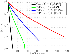
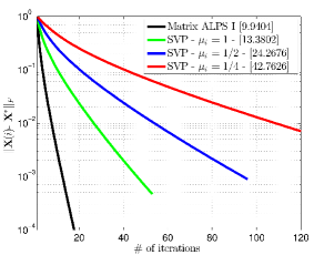
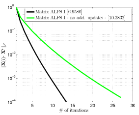
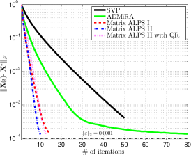
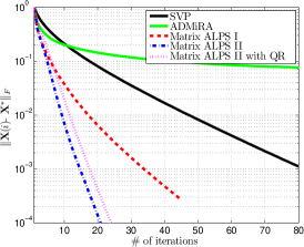
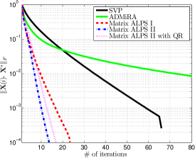
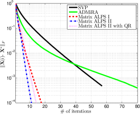
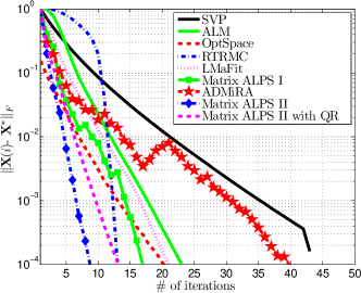
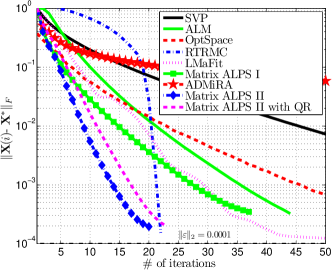
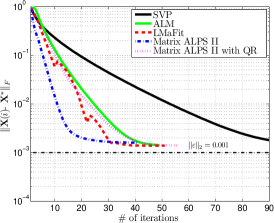
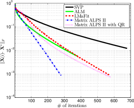
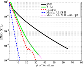
Figure 1: Median error per iteration for various step size policies and 20 Monte-Carlo repetitions. In brackets, we present the median time consumed for convergene in seconds. (a) m=n=2048𝑚𝑛2048m=n=2048, p=0.4n2,𝑝0.4superscript𝑛2p=0.4n^{2}, and rank k=70𝑘70k=70𝓐𝓐\boldsymbol{\mathcal{A}} is formed by permuted and subsampled noiselets coifman2001noiselets . (b) n=2048𝑛2048n=2048 , m=512𝑚512m=512, p=0.4n2𝑝0.4superscript𝑛2p=0.4n^{2}, and rank k=50𝑘50k=50—we use underdetermined linear map 𝓐𝓐\boldsymbol{\mathcal{A}} according to the MC problem (c) n=2048𝑛2048n=2048, m=512𝑚512m=512, p=0.4n2,𝑝0.4superscript𝑛2p=0.4n^{2}, and rank k=40𝑘40k=40—we use underdetermined linear map 𝓐𝓐\boldsymbol{\mathcal{A}} according to the MC problem.

According to Algorithm 1, let 𝑿(i)𝑿𝑖\boldsymbol{X}(i) be the current rank-k𝑘k matrix estimate spanned by the set of orthonormal, rank-1 matrices in 𝒳isubscript𝒳𝑖\mathcal{X}_{i}. Using regular gradient descent motions, the new rank-k𝑘k estimate 𝑾(i)𝑾𝑖\boldsymbol{W}(i) can be calculated through:

𝑽i=𝑿(i)μ2f(𝑿(i)),{𝒲i,𝑾(i)}𝒫k(𝑽(i)).formulae-sequencesubscript𝑽𝑖𝑿𝑖𝜇2𝑓𝑿𝑖subscript𝒲𝑖𝑾𝑖subscript𝒫𝑘𝑽𝑖\displaystyle\boldsymbol{V}_{i}=\boldsymbol{X}(i)-\frac{\mu}{2}\nabla f(\boldsymbol{X}(i)),~{}~{}~{}\{\mathcal{W}_{i},~{}\boldsymbol{W}(i)\}\leftarrow\mathcal{P}_{k}(\boldsymbol{V}(i)).

We highlight that the rank-k𝑘k approximate matrix may not be unique. It then holds that the subspace spanned by 𝒲isubscript𝒲𝑖\mathcal{W}_{i} originates: i)i) either from the subspace of 𝒳isubscript𝒳𝑖\mathcal{X}_{i}, ii)ii) or from the best subspace (in terms of the Frobenius norm metric) of the current gradient f(𝑿(i))𝑓𝑿𝑖\nabla f(\boldsymbol{X}(i)), orthogonal to 𝒳isubscript𝒳𝑖\mathcal{X}_{i}, iii)iii) or from the combination of orthonormal, rank-1 matrices lying on the union of the above two subspaces. The statements above can be summarized in the following expression:

span(𝒲i)span(𝒟i𝒳i)spansubscript𝒲𝑖spansubscript𝒟𝑖subscript𝒳𝑖\displaystyle\text{span}(\mathcal{W}_{i})\in\text{span}\left(\mathcal{D}_{i}\cup\mathcal{X}_{i}\right) (15)

for any step size μisubscript𝜇𝑖\mu_{i} and 𝒟i𝒫k(𝒫𝒳if(𝑿(i)))subscript𝒟𝑖subscript𝒫𝑘subscript𝒫superscriptsubscript𝒳𝑖bottom𝑓𝑿𝑖\mathcal{D}_{i}\leftarrow\mathcal{P}_{k}\big{(}\mathcal{P}_{\mathcal{X}_{i}^{\bot}}\nabla f(\boldsymbol{X}(i))\big{)}. Since rank(span(𝒲i))krankspansubscript𝒲𝑖𝑘\text{rank}(\text{span}(\mathcal{W}_{i}))\leq k, we easily deduce the following key observation: let 𝒮i𝒟i𝒳isubscript𝒮𝑖subscript𝒟𝑖subscript𝒳𝑖\mathcal{S}_{i}\leftarrow\mathcal{D}_{i}\cup\mathcal{X}_{i} be a set of rank-1, orthonormal matrices where rank(span(𝒮i))2krankspansubscript𝒮𝑖2𝑘\text{rank}(\text{span}(\mathcal{S}_{i}))\leq 2k. Given 𝒲isubscript𝒲𝑖\mathcal{W}_{i} is unknown before the i𝑖i-th iteration, 𝒮isubscript𝒮𝑖\mathcal{S}_{i} spans the smallest subspace that contains 𝒲isubscript𝒲𝑖\mathcal{W}_{i} such that the following equality

𝒫ksubscript𝒫𝑘\displaystyle\mathcal{P}_{k} (𝑿(i)μi2f(𝑿(i)))𝑿𝑖subscript𝜇𝑖2𝑓𝑿𝑖\displaystyle\left(\boldsymbol{X}(i)-\frac{\mu_{i}}{2}\nabla f(\boldsymbol{X}(i))\right)
=𝒫k(𝑿(i)μi2𝒫𝒮if(𝑿(i)))absentsubscript𝒫𝑘𝑿𝑖subscript𝜇𝑖2subscript𝒫subscript𝒮𝑖𝑓𝑿𝑖\displaystyle=\mathcal{P}_{k}\left(\boldsymbol{X}(i)-\frac{\mu_{i}}{2}\mathcal{P}_{\mathcal{S}_{i}}\nabla f(\boldsymbol{X}(i))\right) (16)

necessarily holds.222In the case of multiple identical singular values, any ties are lexicographically dissolved.

To compute step-size μisubscript𝜇𝑖\mu_{i}, we use:

μisubscript𝜇𝑖\displaystyle\mu_{i} =argminμ𝒚𝓐(𝑿(i)μ2𝒫𝒮if(𝑿(i)))22absentsubscriptargmin𝜇superscriptsubscriptnorm𝒚𝓐𝑿𝑖𝜇2subscript𝒫subscript𝒮𝑖𝑓𝑿𝑖22\displaystyle=\operatorname*{arg\,min}_{\mu}\big{\|}\boldsymbol{y}-\boldsymbol{\mathcal{A}}\left(\boldsymbol{X}(i)-\frac{\mu}{2}\mathcal{P}_{\mathcal{S}_{i}}\nabla f(\boldsymbol{X}(i))\right)\big{\|}_{2}^{2}
=𝒫𝒮if(𝑿(i))F2𝓐𝒫𝒮if(𝑿(i))22,absentsuperscriptsubscriptnormsubscript𝒫subscript𝒮𝑖𝑓𝑿𝑖𝐹2superscriptsubscriptnorm𝓐subscript𝒫subscript𝒮𝑖𝑓𝑿𝑖22\displaystyle=\frac{\|\mathcal{P}_{\mathcal{S}_{i}}\nabla f(\boldsymbol{X}(i))\|_{F}^{2}}{\|\boldsymbol{\mathcal{A}}\mathcal{P}_{\mathcal{S}_{i}}\nabla f(\boldsymbol{X}(i))\|_{2}^{2}}, (17)

i.e., μisubscript𝜇𝑖\mu_{i} is the minimizer of the objective function, given the current gradient f(𝑿(i))𝑓𝑿𝑖\nabla f(\boldsymbol{X}(i)). Note that:

1δ2k(𝓐)1μi1+δ2k(𝓐),1subscript𝛿2𝑘𝓐1subscript𝜇𝑖1subscript𝛿2𝑘𝓐\displaystyle{}1-\delta_{2k}(\boldsymbol{\mathcal{A}})\leq\frac{1}{\mu_{i}}\leq 1+\delta_{2k}(\boldsymbol{\mathcal{A}}), (18)

due to R-RIP—i.e., we select 2k2𝑘2k subspaces such that μisubscript𝜇𝑖\mu_{i} satisfies (18). We can derive similar arguments for the additional step size selection ξisubscript𝜉𝑖\xi_{i} in Step 6 of Algorithm 1.

Adaptive μisubscript𝜇𝑖\mu_{i} scheme results in more restrictive worst-case isometry constants compared to HTP ; foucart2010sparse ; SVP , but faster convergence and better stability are empirically observed in general. In SVP , the authors present the Singular Value Projection (SVP) algorithm, an iterative hard thresholding algorithm for the ARM problem. According to SVP , both constant and iteration dependent (but user-defined) step sizes are considered. Adaptive strategies presented in SVP require the computation of R-RIP constants which has exponential time complexity. Figures 1(a)-(b) illustrate some characteristic examples. The performance varies for different problem configurations. For μ>1𝜇1\mu>1, SVP diverges for various test cases. We note that, for large fixed matrix dimensions m,n𝑚𝑛m,n, adaptive step size selection becomes computationally expensive compared to constant step size selection strategies, as the rank of 𝑿superscript𝑿\boldsymbol{X}^{\ast} increases.

4.2 Updates on restricted subspaces

In Algorithm 1, at each iteration, the new estimate 𝑾(i)𝒫k(𝑽(i))𝑾𝑖subscript𝒫𝑘𝑽𝑖\boldsymbol{W}(i)\leftarrow\mathcal{P}_{k}\left(\boldsymbol{V}(i)\right) can be further refined by applying a single or multiple gradient descent updates with line search restricted on 𝒲isubscript𝒲𝑖\mathcal{W}_{i} HTP (Step 7 in Algorithm 1):

𝑿(i+1)𝑾(i)ξi2𝒫𝒲if(𝑾(i)),𝑿𝑖1𝑾𝑖subscript𝜉𝑖2subscript𝒫subscript𝒲𝑖𝑓𝑾𝑖\displaystyle\boldsymbol{X}(i+1)\leftarrow\boldsymbol{W}(i)-\frac{\xi_{i}}{2}\mathcal{P}_{\mathcal{W}_{i}}\nabla f(\boldsymbol{W}(i)),

whereξi=𝒫𝒲if(𝑾(i))F2𝓐𝒫𝒲if(𝑾(i))22.wheresubscript𝜉𝑖superscriptsubscriptnormsubscript𝒫subscript𝒲𝑖𝑓𝑾𝑖𝐹2superscriptsubscriptnorm𝓐subscript𝒫subscript𝒲𝑖𝑓𝑾𝑖22\text{where}~{}\xi_{i}=\frac{\|\mathcal{P}_{\mathcal{W}_{i}}\nabla f(\boldsymbol{W}(i))\|_{F}^{2}}{\|\boldsymbol{\mathcal{A}}\mathcal{P}_{\mathcal{W}_{i}}\nabla f(\boldsymbol{W}(i))\|_{2}^{2}}. In spirit, the gradient step above is the same as block coordinate descent in convex optimization where we find the subspaces adaptively. Figure 1(c) depicts the acceleration achieved by using additional gradient updates over restricted low-rank subspaces for a test case.

4.3 Acceleration via memory-based schemes and low-rank matrix approximations

Memory-based techniques can be used to improve convergence speed. Furthermore, low-rank matrix approximation tools overcome the computational overhead of computing the best low-rank projection by inexactly solving (5). We keep the discussion on memory utilization for Section 7 and low-rank matrix approximations for Sections 8 and 9 where we present new algorithmic frameworks for low-rank matrix recovery.


Refer to caption
Refer to caption
Refer to caption
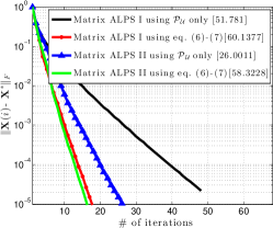
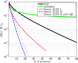
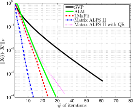
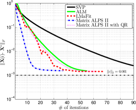
Figure 2: Median error per iteration for Matrix ALPS I and Matrix ALPS II variants over 10 Monte-Carlo repetitions. In brackets, we present the median time consumed for convergene in seconds. (a) n=2048,m=512formulae-sequence𝑛2048𝑚512n=2048,m=512, p=0.25n2,𝑝0.25superscript𝑛2p=0.25n^{2}, and rank k=40𝑘40k=40. (b) n=2000,m=1000formulae-sequence𝑛2000𝑚1000n=2000,m=1000, p=0.25n2,𝑝0.25superscript𝑛2p=0.25n^{2}, and rank k=50𝑘50k=50. (c) n=m=1000𝑛𝑚1000n=m=1000, p=0.25n2,𝑝0.25superscript𝑛2p=0.25n^{2}, and rank k=50𝑘50k=50.

4.4 Active low-rank subspace tracking

Per iteration of Algorithms 1 and 2, we perform projection operations 𝒫𝒮𝑿subscript𝒫𝒮𝑿\mathcal{P}_{\mathcal{S}}\boldsymbol{X} and 𝒫𝒮𝑿subscript𝒫superscript𝒮bottom𝑿\mathcal{P}_{\mathcal{S}^{\bot}}\boldsymbol{X} where 𝑿m×n𝑿superscript𝑚𝑛\boldsymbol{X}\in\mathbb{R}^{m\times n}, as described by (6) and (7), respectively. Since 𝒮𝒮\mathcal{S} is constituted by outer products of left and right singular vectors as in Definition 2, 𝒫𝒮𝑿subscript𝒫𝒮𝑿\mathcal{P}_{\mathcal{S}}\boldsymbol{X} (resp. 𝒫𝒮𝑿subscript𝒫superscript𝒮bottom𝑿\mathcal{P}_{\mathcal{S}^{\bot}}\boldsymbol{X}) projects onto the (resp. complement of the) best low-rank subspace in R(𝑿)𝑅𝑿R(\boldsymbol{X}) and R(𝑿T)𝑅superscript𝑿𝑇R(\boldsymbol{X}^{T}). These operations are highly connected with the adaptive step size selection and the updates on restricted subspaces. Unfortunately, the time-complexity to compute 𝒫𝒮𝑿subscript𝒫𝒮𝑿\mathcal{P}_{\mathcal{S}}\boldsymbol{X} is dominated by three matrix-matrix multiplications which decelerates the convergence of the proposed schemes in high-dimensional settings. To accelerate the convergence in many test cases, it turns out that we do not have to use the best projection 𝒫𝒮subscript𝒫𝒮\mathcal{P}_{\mathcal{S}} in practice.333From a different perspective and for a different problem case, similar ideas have been used in ALM . Rather, employing inexact projections is sufficient to converge to the optimal solution: either i)i) 𝒫𝒰𝑿subscript𝒫𝒰𝑿\mathcal{P}_{\mathcal{U}}\boldsymbol{X} onto the best low-rank subspace in R(𝑿)𝑅𝑿R(\boldsymbol{X}) only (if mnmuch-less-than𝑚𝑛m\ll n) or ii)ii) 𝑿𝒫𝒱𝑿subscript𝒫𝒱\boldsymbol{X}\mathcal{P}_{\mathcal{V}} onto the best low-rank subspace in R(𝑿T)𝑅superscript𝑿𝑇R(\boldsymbol{X}^{T}) only (if mnmuch-greater-than𝑚𝑛m\gg n)444We can move between these two cases by a simple transpose of the problem.; 𝒫𝒰subscript𝒫𝒰\mathcal{P}_{\mathcal{U}} and 𝒫𝒱subscript𝒫𝒱\mathcal{P}_{\mathcal{V}} are defined in Definition 2 and require only one matrix-matrix multiplication.

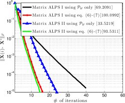
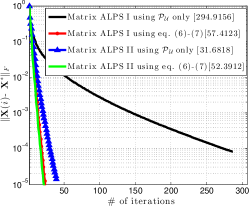
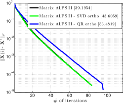
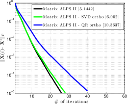
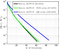
Figure 2 shows the time overhead due to the exact projection application 𝒫𝒮subscript𝒫𝒮\mathcal{P}_{\mathcal{S}} compared to 𝒫𝒰subscript𝒫𝒰\mathcal{P}_{\mathcal{U}} for mn𝑚𝑛m\leq n. In Figure 2(a), we use subsampled and permuted noiselets for linear map 𝓐𝓐\boldsymbol{\mathcal{A}} and in Figures 2(b)-(c), we test the MC problem. While in the case m=n𝑚𝑛m=n the use of (6)-(7) has a clear advantage over inexact projections using only 𝒫𝒰subscript𝒫𝒰\mathcal{P}_{\mathcal{U}}, the latter case converges faster to the desired accuracy 51045superscript1045\cdot 10^{-4} when mnmuch-less-than𝑚𝑛m\ll n as shown in Figures 2(a)-(b). In our derivations, we assume 𝒫𝒮subscript𝒫𝒮\mathcal{P}_{\mathcal{S}} and 𝒫𝒮subscript𝒫superscript𝒮bottom\mathcal{P}_{\mathcal{S}^{\bot}} as defined in (6) and (7).

5 Convergence guarantees

In this section, we present the theoretical convergence guarantees of Algorithms 1 and 2 as functions of R-RIP constants. To characterize the performance of the proposed algorithms, both in terms of convergence rate and noise resilience, we use the following recursive expression:

𝑿(i+1)𝑿Fρ𝑿(i)𝑿F+γ𝜺2.subscriptnorm𝑿𝑖1superscript𝑿𝐹𝜌subscriptnorm𝑿𝑖superscript𝑿𝐹𝛾subscriptnorm𝜺2\displaystyle\|\boldsymbol{X}(i+1)-\boldsymbol{X}^{\ast}\|_{F}\leq\rho\|\boldsymbol{X}(i)-\boldsymbol{X}^{\ast}\|_{F}+\gamma\|\boldsymbol{\varepsilon}\|_{2}. (19)

In (19), γ𝛾\gamma denotes the approximation guarantee and provides insights into algorithm’s reconstruction capabilities when additive noise is present; ρ<1𝜌1\rho<1 expresses the convergence rate towards a region around 𝑿superscript𝑿\boldsymbol{X}^{\ast}, whose radius is determined by γ1ρ𝜺2𝛾1𝜌subscriptnorm𝜺2\frac{\gamma}{1-\rho}\|\boldsymbol{\varepsilon}\|_{2}. In short, (19) characterizes how the distance to the true signal 𝑿superscript𝑿\boldsymbol{X}^{\ast} is decreased and how the noise level affects the accuracy of the solution, at each iteration.

5.1 Matrix ALPS I

An important lemma for our derivations below is given next:

Lemma 6

[Active subspace expansion] Let 𝐗(i)𝐗𝑖\boldsymbol{X}(i) be the matrix estimate at the i𝑖i-th iteration and let 𝒳isubscript𝒳𝑖\mathcal{X}_{i} be a set of orthonormal, rank-1 matrices such that 𝒳i𝒫k(𝐗(i))subscript𝒳𝑖subscript𝒫𝑘𝐗𝑖\mathcal{X}_{i}\leftarrow\mathcal{P}_{k}(\boldsymbol{X}(i)). Then, at each iteration, the Active Subspace Expansion step in Algorithms 1 and 2 identifies information in 𝐗superscript𝐗\boldsymbol{X}^{\ast}, such that:

𝒫𝒳𝒫𝒮i𝑿Fsubscriptnormsubscript𝒫superscript𝒳subscript𝒫superscriptsubscript𝒮𝑖bottomsuperscript𝑿𝐹\displaystyle\big{\|}\mathcal{P}_{\mathcal{X}^{\ast}}\mathcal{P}_{\mathcal{S}_{i}^{\bot}}\boldsymbol{X}^{\ast}\big{\|}_{F} (2δ2k+2δ3k)𝑿(i)𝑿Fabsent2subscript𝛿2𝑘2subscript𝛿3𝑘subscriptnorm𝑿𝑖superscript𝑿𝐹\displaystyle\leq(2\delta_{2k}+2\delta_{3k})\big{\|}\boldsymbol{X}(i)-\boldsymbol{X}^{\ast}\big{\|}_{F}
+2(1+δ2k)𝜺2,21subscript𝛿2𝑘subscriptnorm𝜺2\displaystyle+\sqrt{2(1+\delta_{2k})}\big{\|}\boldsymbol{\varepsilon}\big{\|}_{2}, (20)

where 𝒮i𝒳i𝒟isubscript𝒮𝑖subscript𝒳𝑖subscript𝒟𝑖\mathcal{S}_{i}\leftarrow\mathcal{X}_{i}\cup\mathcal{D}_{i} and 𝒳𝒫k(𝐗)superscript𝒳subscript𝒫𝑘superscript𝐗\mathcal{X}^{\ast}\leftarrow\mathcal{P}_{k}(\boldsymbol{X}^{\ast}).

Lemma 6 states that, at each iteration, the active subspace expansion step identifies a 2k𝑘k rank subspace such that the amount of unrecovered energy of 𝑿superscript𝑿\boldsymbol{X}^{\ast}—i.e., the projection of 𝑿superscript𝑿\boldsymbol{X}^{\ast} onto the orthogonal subspace of span(𝒮i)spansubscript𝒮𝑖\text{span}(\mathcal{S}_{i})—is bounded by (20).

Then, Theorem 1 characterizes the iteration invariant of Algorithm 1 for the matrix case:

Theorem 5.1

[Iteration invariant for Matrix ALPS I] The (i+1)𝑖1(i+1)-th matrix estimate 𝐗(i+1)𝐗𝑖1\boldsymbol{X}(i+1) of Matrix ALPS I satisfies the following recursion:

𝑿(i+1)𝑿Fsubscriptnorm𝑿𝑖1superscript𝑿𝐹\displaystyle\big{\|}\boldsymbol{X}(i+1)-\boldsymbol{X}^{\ast}\big{\|}_{F} ρ𝑿(i)𝑿F+γ𝜺2,absent𝜌subscriptnorm𝑿𝑖superscript𝑿𝐹𝛾subscriptnorm𝜺2\displaystyle\leq\rho\big{\|}\boldsymbol{X}(i)-\boldsymbol{X}^{\ast}\big{\|}_{F}+\gamma\big{\|}\boldsymbol{\varepsilon}\big{\|}_{2}, (21)

where ρ:=(1+2δ2k1δ2k)(4δ2k1δ2k+(2δ2k+2δ3k)2δ3k1δ2k)assign𝜌12subscript𝛿2𝑘1subscript𝛿2𝑘4subscript𝛿2𝑘1subscript𝛿2𝑘2subscript𝛿2𝑘2subscript𝛿3𝑘2subscript𝛿3𝑘1subscript𝛿2𝑘\rho:=\Big{(}\frac{1+2\delta_{2k}}{1-\delta_{2k}}\Big{)}\Big{(}\frac{4\delta_{2k}}{1-\delta_{2k}}+(2\delta_{2k}+2\delta_{3k})\frac{2\delta_{3k}}{1-\delta_{2k}}\Big{)} and γ:=(1+2δ2k1δ2k)(21+δ2k1δ2k+2δ3k1δ2k2(1+δ2k))+1+δk1δk.assign𝛾12subscript𝛿2𝑘1subscript𝛿2𝑘21subscript𝛿2𝑘1subscript𝛿2𝑘2subscript𝛿3𝑘1subscript𝛿2𝑘21subscript𝛿2𝑘1subscript𝛿𝑘1subscript𝛿𝑘\gamma:=\Big{(}\frac{1+2\delta_{2k}}{1-\delta_{2k}}\Big{)}\Big{(}\frac{2\sqrt{1+\delta_{2k}}}{1-\delta_{2k}}+\frac{2\delta_{3k}}{1-\delta_{2k}}\sqrt{2(1+\delta_{2k})}\Big{)}+\frac{\sqrt{1+\delta_{k}}}{1-\delta_{k}}. Moreover, when δ3k<0.1235subscript𝛿3𝑘0.1235\delta_{3k}<0.1235, the iterations are contractive.

To provide some intuition behind this result, assume that 𝑿superscript𝑿\boldsymbol{X}^{\ast} is a rank-k𝑘k matrix. Then, according to Theorem 5.1, for ρ<1𝜌1\rho<1, the approximation parameter γ𝛾\gamma in (21) satisfies:

γ<5.7624,forδ3k<0.1235.formulae-sequence𝛾5.7624forsubscript𝛿3𝑘0.1235\displaystyle\gamma<5.7624,~{}~{}\text{for}~{}~{}\delta_{3k}<0.1235.

Moreover, we derive the following:

ρ<1+2δ3k(1δ3k)2(4δ3k+8δ3k2)<12δ3k<0.079,𝜌12subscript𝛿3𝑘superscript1subscript𝛿3𝑘24subscript𝛿3𝑘8superscriptsubscript𝛿3𝑘212subscript𝛿3𝑘0.079\displaystyle\rho<\frac{1+2\delta_{3k}}{(1-\delta_{3k})^{2}}\big{(}4\delta_{3k}+8\delta_{3k}^{2}\big{)}<\frac{1}{2}\Rightarrow\delta_{3k}<0.079,

which is a stronger R-RIP condition assumption compared to state-of-the-art approaches admira2010 . In the next section, we further improve this guarantee using Algorithm 2.

Unfolding the recursive formula (21), we obtain the following upper bound for 𝑿(i)𝑿Fsubscriptnorm𝑿𝑖superscript𝑿𝐹\big{\|}\boldsymbol{X}(i)-\boldsymbol{X}^{\ast}\big{\|}_{F} at the i𝑖i-th iteration:

𝑿(i)𝑿Fρi𝑿(0)𝑿F+γ1ρ𝜺2.subscriptnorm𝑿𝑖superscript𝑿𝐹superscript𝜌𝑖subscriptnorm𝑿0superscript𝑿𝐹𝛾1𝜌subscriptnorm𝜺2\displaystyle\big{\|}\boldsymbol{X}(i)-\boldsymbol{X}^{\ast}\big{\|}_{F}\leq\rho^{i}\big{\|}\boldsymbol{X}(0)-\boldsymbol{X}^{\ast}\big{\|}_{F}+\frac{\gamma}{1-\rho}\big{\|}\boldsymbol{\varepsilon}\big{\|}_{2}. (22)

Then, given 𝑿(0)=𝟎𝑿00\boldsymbol{X}(0)=\mathbf{0}, Matrix ALPS I finds a rank-k𝑘k solution 𝑿^m×n^𝑿superscript𝑚𝑛\widehat{\boldsymbol{X}}\in\mathbb{R}^{m\times n} such that 𝑿^𝑿Fγ+1ρ1ρ𝜺2subscriptnorm^𝑿superscript𝑿𝐹𝛾1𝜌1𝜌subscriptnorm𝜺2\big{\|}\widehat{\boldsymbol{X}}-\boldsymbol{X}^{\ast}\big{\|}_{F}\leq\frac{\gamma+1-\rho}{1-\rho}\big{\|}\boldsymbol{\varepsilon}\big{\|}_{2} after i:=log(𝑿F/𝜺2)log(1/ρ)assign𝑖subscriptnormsuperscript𝑿𝐹subscriptnorm𝜺21𝜌i:=\Big{\lceil}\frac{\log(\|\boldsymbol{X}^{\ast}\|_{F}/\|\boldsymbol{\varepsilon}\|_{2})}{\log(1/\rho)}\Big{\rceil} iterations.

If we ignore steps 5 and 6 in Algorithm 1, we obtain another projected gradient descent variant for the affine rank minimization problem, for which we obtain the following performance guarantees—the proof follows from the proof of Theorem 5.1.

Corollary 1

[Matrix ALPS I Instance] In Algorithm 1, we ignore steps 5 and 6 and let {𝒳i+1,𝐗(i+1)}𝒫k(𝐕i)subscript𝒳𝑖1𝐗𝑖1subscript𝒫𝑘subscript𝐕𝑖\{\mathcal{X}_{i+1},~{}\boldsymbol{X}(i+1)\}\leftarrow\mathcal{P}_{k}(\boldsymbol{V}_{i}). Then, by the same analysis, we observe that the following recursion is satisfied:

𝑿(i+1)𝑿Fsubscriptnorm𝑿𝑖1superscript𝑿𝐹\displaystyle\big{\|}\boldsymbol{X}(i+1)-\boldsymbol{X}^{\ast}\big{\|}_{F} ρ𝑿(i)𝑿F+γ𝜺2,absent𝜌subscriptnorm𝑿𝑖superscript𝑿𝐹𝛾subscriptnorm𝜺2\displaystyle\leq\rho\big{\|}\boldsymbol{X}(i)-\boldsymbol{X}^{\ast}\big{\|}_{F}+\gamma\big{\|}\boldsymbol{\varepsilon}\big{\|}_{2}, (23)

for ρ:=(4δ2k1δ2k+(2δ2k+2δ3k)2δ3k1δ2k)assign𝜌4subscript𝛿2𝑘1subscript𝛿2𝑘2subscript𝛿2𝑘2subscript𝛿3𝑘2subscript𝛿3𝑘1subscript𝛿2𝑘\rho:=\Big{(}\frac{4\delta_{2k}}{1-\delta_{2k}}+(2\delta_{2k}+2\delta_{3k})\frac{2\delta_{3k}}{1-\delta_{2k}}\Big{)} and γ:=(21+δ2k1δ2k+2δ3k1δ2k2(1+δ2k))assign𝛾21subscript𝛿2𝑘1subscript𝛿2𝑘2subscript𝛿3𝑘1subscript𝛿2𝑘21subscript𝛿2𝑘\gamma:=\Big{(}\frac{2\sqrt{1+\delta_{2k}}}{1-\delta_{2k}}+\frac{2\delta_{3k}}{1-\delta_{2k}}\sqrt{2(1+\delta_{2k})}\Big{)}. Moreover, ρ<1𝜌1\rho<1 when δ3k<0.1594subscript𝛿3𝑘0.1594\delta_{3k}<0.1594.

We observe that the absence of the additional estimate update over restricted support sets results in less restrictive isometry constants compared to Theorem 5.1. In practice, additional updates result in faster convergence, as shown in Figure 1(c).

5.2 ADMiRA Instance

In Matrix ALPS I, the gradient descent steps constitute a first-order approximation to least-squares minimization problems. Replacing Step 4 in Algorithm 1 with the following optimization problem:

𝑽(i)argmin𝑽:𝑽span(𝒮i)𝒚𝓐𝑽22,𝑽𝑖subscriptargmin:𝑽𝑽spansubscript𝒮𝑖superscriptsubscriptnorm𝒚𝓐𝑽22\displaystyle\boldsymbol{V}(i)\leftarrow\operatorname*{arg\,min}_{\boldsymbol{V}:\boldsymbol{V}\in\text{span}(\mathcal{S}_{i})}\big{\|}\boldsymbol{y}-\boldsymbol{\mathcal{A}}\boldsymbol{V}\big{\|}_{2}^{2}, (24)

we obtain ADMiRA (furthermore, we remove the de-bias step in Algorithm 1). Assuming that the linear operator 𝓐𝓐\boldsymbol{\mathcal{A}}, restricted on sufficiently low-rank subspaces, is well conditioned in terms of the R-RIP assumption, the optimization problem (24) has a unique optimal minimizer. By exploiting the optimality condition in Lemma 1, ADMiRA instance in Algorithm 2 features the following guarantee:

Theorem 5.2

[Iteration invariant for ADMiRA instance] The (i+1)𝑖1(i+1)-th matrix estimate 𝐗(i+1)𝐗𝑖1\boldsymbol{X}(i+1) of ADMiRA answers the following recursive expression:

𝑿(i+1)𝑿Fρ𝑿(i)𝑿F+γ𝜺F,subscriptnorm𝑿𝑖1superscript𝑿𝐹𝜌subscriptnorm𝑿𝑖superscript𝑿𝐹𝛾subscriptnorm𝜺𝐹\big{\|}\boldsymbol{X}(i+1)-\boldsymbol{X}^{\ast}\big{\|}_{F}\leq\rho\big{\|}\boldsymbol{X}(i)-\boldsymbol{X}^{\ast}\big{\|}_{F}+\gamma\big{\|}\boldsymbol{\varepsilon}\big{\|}_{F},

ρ:=(2δ2k+2δ3k)1+3δ3k21δ3k2,assign𝜌2subscript𝛿2𝑘2subscript𝛿3𝑘13superscriptsubscript𝛿3𝑘21superscriptsubscript𝛿3𝑘2\rho:=\big{(}2\delta_{2k}+2\delta_{3k}\big{)}\sqrt{\frac{1+3\delta_{3k}^{2}}{1-\delta_{3k}^{2}}}, and γ:=1+3δ3k21δ3k22(1+δ3k)assign𝛾13superscriptsubscript𝛿3𝑘21superscriptsubscript𝛿3𝑘221subscript𝛿3𝑘\gamma:=\sqrt{\frac{1+3\delta_{3k}^{2}}{1-\delta_{3k}^{2}}}\sqrt{2(1+\delta_{3k})} +(1+3δ3k21δ3k+3)1+δ2k.13superscriptsubscript𝛿3𝑘21subscript𝛿3𝑘31subscript𝛿2𝑘+\Big{(}\frac{\sqrt{1+3\delta_{3k}^{2}}}{1-\delta_{3k}}+\sqrt{3}\Big{)}\sqrt{1+\delta_{2k}}. Moreover, when δ3k<0.2267subscript𝛿3𝑘0.2267\delta_{3k}<0.2267, the iterations are contractive.

Similarly to Matrix ALPS I analysis, the parameter γ𝛾\gamma in Theorem 5.2 satisfies:

γ<5.1848,forδ3k<0.2267.formulae-sequence𝛾5.1848forsubscript𝛿3𝑘0.2267\displaystyle\gamma<5.1848,~{}\text{for}~{}\delta_{3k}<0.2267.

Furthermore, to compare the approximation guarantees of Theorem 5.2 with admira2010 , we further observe:

δ3k<0.1214,forρ<1/2.formulae-sequencesubscript𝛿3𝑘0.1214for𝜌12\displaystyle\delta_{3k}<0.1214,~{}\text{for}~{}\rho<1/2.

We remind that admira2010 provides convergence guarantees for ADMiRA with δ4k<0.04subscript𝛿4𝑘0.04\delta_{4k}<0.04 for ρ=1/2𝜌12\rho=1/2.

6 Complexity Analysis

In each iteration, computational requirements of the proposed hard thresholding methods mainly depend on the total number of linear mapping operations 𝓐𝓐\boldsymbol{\mathcal{A}}, gradient descent steps, least-squares optimizations, projection operations and matrix decompositions for low rank approximation. Different algorithmic configurations (e.g. removing steps 6 and 7 in Algorithm 1) lead to hard thresholding variants with less computational complexity per iteration and better R-RIP conditions for convergence but a degraded performance in terms of stability and convergence speed is observed in practice. On the other hand, these additional processing steps increase the required time-complexity per iteration; hence, low iteration counts are desired to tradeoff these operations.

A non-exhaustive list of linear map examples includes the identity operator (Principal component analysis (PCA) problem), Fourier/Wavelets/Noiselets tranformations and the famous Matrix Completion problem where 𝓐𝓐\boldsymbol{\mathcal{A}} is a mask operator such that only a fraction of elements in 𝑿𝑿\boldsymbol{X} is observed. Assuming the most demanding case where 𝓐𝓐\boldsymbol{\mathcal{A}} and 𝓐superscript𝓐\boldsymbol{\mathcal{A}}^{\ast} are dense linear maps with no structure, the computation of the gradient f(𝑿(i))𝑓𝑿𝑖\nabla f(\boldsymbol{X}(i)) at each iteration requires O(pkmn)𝑂𝑝𝑘𝑚𝑛O(pkmn) arithmetic operations.

Given a set 𝒮𝒮\mathcal{S} of orthonormal, rank-1 matrices, the projection 𝒫𝒮𝑿subscript𝒫𝒮𝑿\mathcal{P}_{\mathcal{S}}\boldsymbol{X} for any matrix 𝑿m×n𝑿superscript𝑚𝑛\boldsymbol{X}\in\mathbb{R}^{m\times n} requires time complexity O(max{m2n,O(\max\{m^{2}n, mn2})mn^{2}\}) as a sequence of matrix-matrix multiplication operations.555While such operation has O(max{m2n,O(\max\{m^{2}n, mn2})mn^{2}\}) complexity, each application of 𝒫𝒮𝑿subscript𝒫𝒮𝑿\mathcal{P}_{\mathcal{S}}\boldsymbol{X} requires three matrix-matrix multiplications. To reduce such computational cost, we relax this operation in Section 10 where in practice we use only 𝒫𝒰subscript𝒫𝒰\mathcal{P}_{\mathcal{U}} that needs one matrix-matrix multiplication. In Matrix ALPS I, the adaptive step size selection steps require O(max{pkmn,m2n})𝑂𝑝𝑘𝑚𝑛superscript𝑚2𝑛O(\max\{pkmn,m^{2}n\}) time complexity for the calculation of μisubscript𝜇𝑖\mu_{i} and ξisubscript𝜉𝑖\xi_{i} quantities. In ADMiRA solving a least-squares system restricted on rank-2k𝑘k and rank-k𝑘k subspaces requires O(pk2)𝑂𝑝superscript𝑘2O(pk^{2}) complexity; according to cosamp , admira2010 , the complexity of this step can be further reduced using iterative techniques such as the Richardson method or conjugate gradients algorithm.

Using the Lanczos method, we require O(kmn)𝑂𝑘𝑚𝑛O(kmn) arithmetic operations to compute a rank-k𝑘k matrix approximation for a given constant accuracy; a prohibitive time-complexity that does not scale well for many practical applications. Sections 8 and 9 describe approximate low rank matrix projections and how they affect the convergence guarantees of the proposed algorithms.

Overall, the operation that dominates per iteration requires O(max{pkmn,m2n,mn2})𝑂𝑝𝑘𝑚𝑛superscript𝑚2𝑛𝑚superscript𝑛2O(\max\{pkmn,m^{2}n,mn^{2}\}) time complexity in the proposed schemes.

7 Memory-based Acceleration

Iterative algorithms can use memory to gain momentum in convergence. Based on Nesterov’s optimal gradient methods nesterov2007gradient , we propose a hard thresholding variant, described in Algorithm 3 where an additional update on 𝑿(i+1)𝑿𝑖1\boldsymbol{X}(i+1) with momentum step size τisubscript𝜏𝑖\tau_{i} is performed using previous matrix estimates.

1:Input: 𝒚𝒚\boldsymbol{y}, 𝓐𝓐\boldsymbol{\mathcal{A}}, k𝑘k, Tolerance η𝜂\eta, MaxIterations
2:Initialize: 𝑿(0)0𝑿00\boldsymbol{X}(0)\leftarrow 0, 𝒳0{}subscript𝒳0\mathcal{X}_{0}\leftarrow\{\emptyset\}, 𝑸(0)0𝑸00\boldsymbol{Q}(0)\leftarrow 0, 𝒬0{}subscript𝒬0\mathcal{Q}_{0}\leftarrow\{\emptyset\}, τiisubscript𝜏𝑖for-all𝑖\tau_{i}~{}\forall i, i0𝑖0i\leftarrow 0
3:repeat
4:   𝒟i𝒫k(𝒫𝒬if(𝑸(i)))subscript𝒟𝑖subscript𝒫𝑘subscript𝒫superscriptsubscript𝒬𝑖bottom𝑓𝑸𝑖\mathcal{D}_{i}\leftarrow\mathcal{P}_{k}\big{(}\mathcal{P}_{\mathcal{Q}_{i}^{\bot}}\nabla f(\boldsymbol{Q}(i))\big{)} (Best rank-k𝑘k subspace orthogonal to 𝒬isubscript𝒬𝑖\mathcal{Q}_{i})         
5:   𝒮i𝒟i𝒬isubscript𝒮𝑖subscript𝒟𝑖subscript𝒬𝑖\mathcal{S}_{i}\leftarrow\mathcal{D}_{i}\cup\mathcal{Q}_{i} (Active subspace expansion)         
6:   μiargminμ𝒚𝓐(𝑸(i)μ2𝒫𝒮if(𝑸(i)))22=𝒫𝒮if(𝑸(i))F2𝓐𝒫𝒮if(𝑸(i))22subscript𝜇𝑖subscriptargmin𝜇superscriptsubscriptnorm𝒚𝓐𝑸𝑖𝜇2subscript𝒫subscript𝒮𝑖𝑓𝑸𝑖22superscriptsubscriptnormsubscript𝒫subscript𝒮𝑖𝑓𝑸𝑖𝐹2superscriptsubscriptnorm𝓐subscript𝒫subscript𝒮𝑖𝑓𝑸𝑖22\mu_{i}\leftarrow\operatorname*{arg\,min}_{\mu}\big{\|}\boldsymbol{y}-\boldsymbol{\mathcal{A}}\big{(}\boldsymbol{Q}(i)-\frac{\mu}{2}\mathcal{P}_{\mathcal{S}_{i}}\nabla f(\boldsymbol{Q}(i))\big{)}\big{\|}_{2}^{2}=\frac{\|\mathcal{P}_{\mathcal{S}_{i}}\nabla f(\boldsymbol{Q}(i))\|_{F}^{2}}{\|\boldsymbol{\mathcal{A}}\mathcal{P}_{\mathcal{S}_{i}}\nabla f(\boldsymbol{Q}(i))\|_{2}^{2}} (Step size selection)         
7:   𝑽(i)𝑸(i)μi2𝒫𝒮if(𝑸(i))𝑽𝑖𝑸𝑖subscript𝜇𝑖2subscript𝒫subscript𝒮𝑖𝑓𝑸𝑖\boldsymbol{V}(i)\leftarrow\boldsymbol{Q}(i)-\frac{\mu_{i}}{2}\mathcal{P}_{\mathcal{S}_{i}}\nabla f(\boldsymbol{Q}(i)) (Error norm reduction via gradient descent)         
8:   {𝒳i+1,𝑿(i+1)}𝒫k(𝑽(i))subscript𝒳𝑖1𝑿𝑖1subscript𝒫𝑘𝑽𝑖\{\mathcal{X}_{i+1},~{}\boldsymbol{X}(i+1)\}\leftarrow\mathcal{P}_{k}(\boldsymbol{V}(i)) (Best rank-k𝑘k subspace selection)         
9:   𝑸(i+1)𝑿(i+1)+τi(𝑿(i+1)𝑿(i))𝑸𝑖1𝑿𝑖1subscript𝜏𝑖𝑿𝑖1𝑿𝑖\boldsymbol{Q}(i+1)\leftarrow\boldsymbol{X}(i+1)+\tau_{i}(\boldsymbol{X}(i+1)-\boldsymbol{X}(i)) (Momentum update)         
10:   𝒬i+1ortho(𝒳i𝒳i+1)subscript𝒬𝑖1orthosubscript𝒳𝑖subscript𝒳𝑖1\mathcal{Q}_{i+1}\leftarrow\text{ortho}(\mathcal{X}_{i}\cup\mathcal{X}_{i+1})
11:   ii+1𝑖𝑖1i\leftarrow i+1
12:until 𝑿(i)𝑿(i1)2η𝑿(i)2subscriptnorm𝑿𝑖𝑿𝑖12𝜂subscriptnorm𝑿𝑖2\|\boldsymbol{X}(i)-\boldsymbol{X}(i-1)\|_{2}\leq\eta\|\boldsymbol{X}(i)\|_{2} or MaxIterations.
Algorithm 3 Matrix ALPS II

Similar to μisubscript𝜇𝑖\mu_{i} strategies, τisubscript𝜏𝑖\tau_{i} can be preset as constant or adaptively computed at each iteration. Constant momentum step size selection has no additional computational cost but convergence rate acceleration is not guaranteed for some problem formulations in practice. On the other hand, empirical evidence has shown that adaptive τisubscript𝜏𝑖\tau_{i} selection strategies result in faster convergence compared to zero-memory methods with similar complexity.

For the case of strongly convex objective functions, Nesterov nesterov proposed the following constant momentum step size selection scheme: τi=αi(1αi)αi2+αi+1subscript𝜏𝑖subscript𝛼𝑖1subscript𝛼𝑖superscriptsubscript𝛼𝑖2subscript𝛼𝑖1\tau_{i}=\frac{\alpha_{i}(1-\alpha_{i})}{\alpha_{i}^{2}+\alpha_{i+1}}, where α0(0,1)subscript𝛼001\alpha_{0}\in(0,1) and αi+1subscript𝛼𝑖1\alpha_{i+1} is computed as the root (0,1)absent01\in(0,1) of

αi+12=(1αi+1)αi2+qαi+1,forq1κ2(𝓐),formulae-sequencesuperscriptsubscript𝛼𝑖121subscript𝛼𝑖1superscriptsubscript𝛼𝑖2𝑞subscript𝛼𝑖1for𝑞1superscript𝜅2𝓐\displaystyle\alpha_{i+1}^{2}=(1-\alpha_{i+1})\alpha_{i}^{2}+q\alpha_{i+1},~{}\text{for}~{}~{}q\triangleq\frac{1}{\kappa^{2}(\boldsymbol{\mathcal{A}})}, (25)

where κ(𝓐)𝜅𝓐\kappa(\boldsymbol{\mathcal{A}}) denotes the condition number of 𝓐𝓐\boldsymbol{\mathcal{A}}. In this scheme, exact calculation of q𝑞q parameter is computationally expensive for large-scale data problems and approximation schemes are leveraged to compensate this complexity bottleneck.

Based upon adaptive μisubscript𝜇𝑖\mu_{i} selection, we propose to select τisubscript𝜏𝑖\tau_{i} as the minimizer of the objective function:

τisubscript𝜏𝑖\displaystyle\tau_{i} =argminτ𝒚𝓐𝑸(i+1)22absentsubscriptargmin𝜏superscriptsubscriptnorm𝒚𝓐𝑸𝑖122\displaystyle=\operatorname*{arg\,min}_{\tau}\|\boldsymbol{y}-\boldsymbol{\mathcal{A}}\boldsymbol{Q}(i+1)\|_{2}^{2}
=𝒚𝓐𝑿(i),𝓐𝑿(i)𝓐𝑿(i1)𝓐𝑿(i)𝓐𝑿(i1)22,absent𝒚𝓐𝑿𝑖𝓐𝑿𝑖𝓐𝑿𝑖1superscriptsubscriptnorm𝓐𝑿𝑖𝓐𝑿𝑖122\displaystyle=\frac{\langle\boldsymbol{y}-\boldsymbol{\mathcal{A}}\boldsymbol{X}(i),\boldsymbol{\mathcal{A}}\boldsymbol{X}(i)-\boldsymbol{\mathcal{A}}\boldsymbol{X}(i-1)\rangle}{\|\boldsymbol{\mathcal{A}}\boldsymbol{X}(i)-\boldsymbol{\mathcal{A}}\boldsymbol{X}(i-1)\|_{2}^{2}}, (26)

where 𝓐𝑿(i),𝓐𝑿(i1)𝓐𝑿𝑖𝓐𝑿𝑖1\boldsymbol{\mathcal{A}}\boldsymbol{X}(i),\boldsymbol{\mathcal{A}}\boldsymbol{X}(i-1) are already pre-computed at each iteration. According to (26), τisubscript𝜏𝑖\tau_{i} is dominated by the calculation of a vector inner product, a computationally cheaper process than q𝑞q calculation.

Theorem 7.1 characterizes Algorithm 3 for constant momentum step size selection. To keep the main ideas simple, we ignore the additional gradient updates in Algorithm 3. In addition, we only consider the noiseless case for clarity. The convergence rate proof for these cases is provided in the appendix.

Theorem 7.1

[Iteration invariant for Matrix ALPS II] Let 𝐲=𝓐𝐗𝐲𝓐superscript𝐗\boldsymbol{y}=\boldsymbol{\mathcal{A}}\boldsymbol{X}^{\ast} be a noiseless set of observations. To recover 𝐗superscript𝐗\boldsymbol{X}^{\ast} from 𝐲𝐲\boldsymbol{y} and 𝓐𝓐\boldsymbol{\mathcal{A}}, the (i+1)𝑖1(i+1)-th matrix estimate 𝐗(i+1)𝐗𝑖1\boldsymbol{X}(i+1) of Matrix ALPS II satisfies the following recursion:

𝑿(i+1)𝑿Fsubscriptnorm𝑿𝑖1superscript𝑿𝐹\displaystyle\big{\|}\boldsymbol{X}(i+1)-\boldsymbol{X}^{\ast}\big{\|}_{F} α(1+τi)𝑿(i)𝑿Fabsent𝛼1subscript𝜏𝑖subscriptnorm𝑿𝑖superscript𝑿𝐹\displaystyle\leq\alpha(1+\tau_{i})\big{\|}\boldsymbol{X}(i)-\boldsymbol{X}^{\ast}\big{\|}_{F}
+ατi𝑿(i1)𝑿F,𝛼subscript𝜏𝑖subscriptnorm𝑿𝑖1superscript𝑿𝐹\displaystyle+\alpha\tau_{i}\big{\|}\boldsymbol{X}(i-1)-\boldsymbol{X}^{\ast}\big{\|}_{F}, (27)

where α:=4δ3k1δ3k+(2δ3k+2δ4k)2δ3k1δ3kassign𝛼4subscript𝛿3𝑘1subscript𝛿3𝑘2subscript𝛿3𝑘2subscript𝛿4𝑘2subscript𝛿3𝑘1subscript𝛿3𝑘\alpha:=\frac{4\delta_{3k}}{1-\delta_{3k}}+(2\delta_{3k}+2\delta_{4k})\frac{2\delta_{3k}}{1-\delta_{3k}}. Moreover, solving the above second-order recurrence, the following inequality holds true:

𝑿(i+1)𝑿Fρi+1𝑿(0)𝑿F,subscriptnorm𝑿𝑖1superscript𝑿𝐹superscript𝜌𝑖1subscriptnorm𝑿0superscript𝑿𝐹\displaystyle\big{\|}\boldsymbol{X}(i+1)-\boldsymbol{X}^{\ast}\big{\|}_{F}\leq\rho^{i+1}\big{\|}\boldsymbol{X}(0)-\boldsymbol{X}^{\ast}\big{\|}_{F}, (28)

for ρ:=α(1+τi)+α2(1+τi)2+4ατi2assign𝜌𝛼1subscript𝜏𝑖superscript𝛼2superscript1subscript𝜏𝑖24𝛼subscript𝜏𝑖2\rho:=\frac{\alpha(1+\tau_{i})+\sqrt{\alpha^{2}(1+\tau_{i})^{2}+4\alpha\tau_{i}}}{2}.


Refer to caption
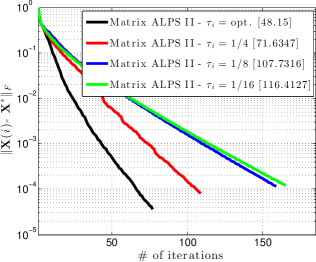
Figure 3: Median error per iteration for various momentum step size policies and 10 Monte-Carlo repetitions. Here, n=1024𝑛1024n=1024, m=256𝑚256m=256, p=0.25n2,𝑝0.25superscript𝑛2p=0.25n^{2}, and rank k=40𝑘40k=40. We use permuted and subsampled noiselets for the linear map 𝓐𝓐\boldsymbol{\mathcal{A}}. In brackets, we present the median time for convergence in seconds.

Theorem 7.1 provides convergence rate behaviour proof for the case where τisubscript𝜏𝑖\tau_{i} is constant ifor-all𝑖\forall i. The more elaborate case where τisubscript𝜏𝑖\tau_{i} follows the policy described in (26) is left as an open question for future work. To provide some insight for (28), for τi=1/4,isubscript𝜏𝑖14for-all𝑖\tau_{i}=1/4,~{}\forall i and τi=1/2,isubscript𝜏𝑖12for-all𝑖\tau_{i}=1/2,~{}\forall i, δ4k<0.1187subscript𝛿4𝑘0.1187\delta_{4k}<0.1187 and δ4k<0.095subscript𝛿4𝑘0.095\delta_{4k}<0.095 guarantee convergence in Algorithm 3, respectively. While the RIP requirements for memory-based Matrix ALPS II are more stringent than the schemes proposed in the previous section, it outperforms Algorithms 1 and 2. Figure 2 shows the acceleration achieved in Matrix ALPS II by using inexact projections 𝒫𝒰subscript𝒫𝒰\mathcal{P}_{\mathcal{U}}. Using the proper projections (6)-(7), Figure 3 shows acceleration in practice when using the adaptive momentum step size strategy: while a wide range of constant momentum step sizes leads to convergence, providing flexibility to select an appropriate τisubscript𝜏𝑖\tau_{i}, adaptive τisubscript𝜏𝑖\tau_{i} avoids this arbitrary τisubscript𝜏𝑖\tau_{i} selection while further decreases the number of iterations needed for convergence in most cases.

8 Accelerating Matrix ALPS: ϵitalic-ϵ\epsilon-Approximation of SVD via Column Subset Selection

A time-complexity bottleneck in the proposed schemes is the computation of the singular value decomposition to find subspaces that describe the unexplored information in matrix 𝑿superscript𝑿\boldsymbol{X}^{\ast}. Unfortunately, the computational cost of regular SVD for best subspace tracking is prohibitive for many applications.

Based on drineas1 ; drineas2 , we can obtain randomized SVD approximations of a matrix 𝑿𝑿\boldsymbol{X} using column subset selection ideas: we compute a leverage score for each column that represents its “significance”. In particular, we define a probability distribution that weights each column depending on the amount of information they contain; usually, the distribution is related to the 2subscript2\ell_{2}-norm of the columns. The main idea of this approach is to compute a surrogate rank-k𝑘k matrix 𝒫kϵ(𝑿)superscriptsubscript𝒫𝑘italic-ϵ𝑿\mathcal{P}_{k}^{\epsilon}(\boldsymbol{X}) by subsampling the columns according to this distribution. It turns out that the total number of sampled columns is a function of the parameter ϵitalic-ϵ\epsilon. Moreover, deshpande1 ; deshpande2 proved that, given a target rank k𝑘k and an approximation parameter ϵitalic-ϵ\epsilon, we can compute an ϵitalic-ϵ\epsilon-approximate rank-k𝑘k matrix 𝒫kϵ(𝑿)superscriptsubscript𝒫𝑘italic-ϵ𝑿\mathcal{P}_{k}^{\epsilon}(\boldsymbol{X}) according to the following defintion.

Definition 4

[ϵitalic-ϵ\epsilon-approximate low-rank projection] Let 𝑿𝑿\boldsymbol{X} be an arbitrary matrix. Then, 𝒫kϵ(𝑿)superscriptsubscript𝒫𝑘italic-ϵ𝑿\mathcal{P}_{k}^{\epsilon}(\boldsymbol{X}) projection provides a rank-k𝑘k matrix approximation to 𝑿𝑿\boldsymbol{X} such that:

𝒫kϵ(𝑿)𝑿F2(1+ϵ)𝒫k(𝑿)𝑿F2,superscriptsubscriptnormsuperscriptsubscript𝒫𝑘italic-ϵ𝑿𝑿𝐹21italic-ϵsuperscriptsubscriptnormsubscript𝒫𝑘𝑿𝑿𝐹2\displaystyle\big{\|}\mathcal{P}_{k}^{\epsilon}(\boldsymbol{X})-\boldsymbol{X}\big{\|}_{F}^{2}\leq(1+\epsilon)\big{\|}\mathcal{P}_{k}(\boldsymbol{X})-\boldsymbol{X}\big{\|}_{F}^{2}, (29)

where 𝒫k(𝑿)argmin𝒀:rank(𝒀)k𝑿𝒀Fsubscript𝒫𝑘𝑿subscriptargmin:𝒀rank𝒀𝑘subscriptnorm𝑿𝒀𝐹\mathcal{P}_{k}(\boldsymbol{X})\in\operatorname*{arg\,min}_{\boldsymbol{Y}:\text{rank}(\boldsymbol{Y})\leq k}\|\boldsymbol{X}-\boldsymbol{Y}\|_{F}.

For the following theoretical results, we assume the following condition on the sensing operator 𝓐::𝓐absent\boldsymbol{\mathcal{A}}: 𝓐𝜷Fλ,𝜷pformulae-sequencesubscriptnormsuperscript𝓐𝜷𝐹𝜆for-all𝜷superscript𝑝\big{\|}\boldsymbol{\mathcal{A}}^{\ast}\boldsymbol{\beta}\big{\|}_{F}\leq\lambda,~{}\forall\boldsymbol{\beta}\in\mathbb{R}^{p} where λ>0𝜆0\lambda>0. Using ϵitalic-ϵ\epsilon-approximation schemes to perform the Active subspace selection step, the following upper bound holds. The proof is provided in the Appendix:

Lemma 7

[ϵitalic-ϵ\epsilon-approximate active subspace expansion] Let 𝐗(i)𝐗𝑖\boldsymbol{X}(i) be the matrix estimate at the i𝑖i-th iteration and let 𝒳isubscript𝒳𝑖\mathcal{X}_{i} be a set of orthonormal, rank-1 matrices in m×nsuperscript𝑚𝑛\mathbb{R}^{m\times n} such that 𝒳i𝒫k(𝐗(i))subscript𝒳𝑖subscript𝒫𝑘𝐗𝑖\mathcal{X}_{i}\leftarrow\mathcal{P}_{k}(\boldsymbol{X}(i)). Furthermore, let

𝒟iϵ𝒫kϵ(𝒫𝒳if(𝑿(i))),superscriptsubscript𝒟𝑖italic-ϵsuperscriptsubscript𝒫𝑘italic-ϵsubscript𝒫superscriptsubscript𝒳𝑖bottom𝑓𝑿𝑖\displaystyle\mathcal{D}_{i}^{\epsilon}\leftarrow\mathcal{P}_{k}^{\epsilon}\big{(}\mathcal{P}_{\mathcal{X}_{i}^{\bot}}\nabla f(\boldsymbol{X}(i))\big{)},

be a set of orthonormal, rank-1 matrices that span rank-k𝑘k subspace such that (29) is satisfied for 𝐗:=𝒫𝒳if(𝐗(i))assign𝐗subscript𝒫superscriptsubscript𝒳𝑖bottom𝑓𝐗𝑖\boldsymbol{X}:=\mathcal{P}_{\mathcal{X}_{i}^{\bot}}\nabla f(\boldsymbol{X}(i)). Then, at each iteration, the Active Subspace Expansion step in Algorithms 1 and 2 captures information contained in the true matrix 𝐗superscript𝐗\boldsymbol{X}^{\ast}, such that:

\displaystyle\big{\|} 𝒫𝒳𝒫𝒮i𝑿Fevaluated-atsubscript𝒫superscript𝒳subscript𝒫superscriptsubscript𝒮𝑖bottomsuperscript𝑿𝐹\displaystyle\mathcal{P}_{\mathcal{X}^{\ast}}\mathcal{P}_{\mathcal{S}_{i}^{\bot}}\boldsymbol{X}^{\ast}\big{\|}_{F}
(2δ2k+2δ3k)𝑿(i)𝑿F+2(1+δ2k)𝜺2absent2subscript𝛿2𝑘2subscript𝛿3𝑘subscriptnorm𝑿𝑖superscript𝑿𝐹21subscript𝛿2𝑘subscriptnorm𝜺2\displaystyle\leq\big{(}2\delta_{2k}+2\delta_{3k}\big{)}\big{\|}\boldsymbol{X}(i)-\boldsymbol{X}^{\ast}\big{\|}_{F}+\sqrt{2(1+\delta_{2k})}\big{\|}\boldsymbol{\varepsilon}\big{\|}_{2}
+2λϵ,2𝜆italic-ϵ\displaystyle+2\lambda\sqrt{\epsilon}, (30)

where 𝒮i𝒳i𝒟iϵsubscript𝒮𝑖subscript𝒳𝑖superscriptsubscript𝒟𝑖italic-ϵ\mathcal{S}_{i}\leftarrow\mathcal{X}_{i}\cup\mathcal{D}_{i}^{\epsilon} and 𝒳𝒫k(𝐗)superscript𝒳subscript𝒫𝑘superscript𝐗\mathcal{X}^{\ast}\leftarrow\mathcal{P}_{k}(\boldsymbol{X}^{\ast}).

Furthermore, to prove the following theorems, we extend Lemma 10, provided in the Appendix, as follows. The proof easily follows from the proof of Lemma 10, using Definition 4:

Lemma 8

[ϵitalic-ϵ\epsilon-approximation rank-k𝑘k subspace selection] Let 𝐕(i)𝐕𝑖\boldsymbol{V}(i) be a rank-2k2𝑘2k proxy matrix in the subspace spanned by 𝒮isubscript𝒮𝑖\mathcal{S}_{i} and let 𝐖^(i)𝒫kϵ(𝐕(i))^𝐖𝑖superscriptsubscript𝒫𝑘italic-ϵ𝐕𝑖\widehat{\boldsymbol{W}}(i)\leftarrow\mathcal{P}_{k}^{\epsilon}(\boldsymbol{V}(i)) denote the rank-k𝑘k ϵitalic-ϵ\epsilon-approxi- mation to 𝐕(i)𝐕𝑖\boldsymbol{V}(i), according to (5). Then:

𝑾^(i)𝑽(i)F2superscriptsubscriptnorm^𝑾𝑖𝑽𝑖𝐹2\displaystyle\big{\|}\widehat{\boldsymbol{W}}(i)-\boldsymbol{V}(i)\big{\|}_{F}^{2} (1+ϵ)𝑾(i)𝑽(i)Fabsent1italic-ϵsubscriptnorm𝑾𝑖𝑽𝑖𝐹\displaystyle\leq(1+\epsilon)\big{\|}\boldsymbol{W}(i)-\boldsymbol{V}(i)\big{\|}_{F}
(1+ϵ)𝒫𝒮i(𝑽(i)𝑿)Fabsent1italic-ϵsubscriptnormsubscript𝒫subscript𝒮𝑖𝑽𝑖superscript𝑿𝐹\displaystyle\leq(1+\epsilon)\big{\|}\mathcal{P}_{\mathcal{S}_{i}}(\boldsymbol{V}(i)-\boldsymbol{X}^{\ast})\big{\|}_{F}
(1+ϵ)𝑽(i)𝑿Fabsent1italic-ϵsubscriptnorm𝑽𝑖superscript𝑿𝐹\displaystyle\leq(1+\epsilon)\big{\|}\boldsymbol{V}(i)-\boldsymbol{X}^{\ast}\big{\|}_{F} (31)

where 𝐖(i)𝒫k(𝐕(i))𝐖𝑖subscript𝒫𝑘𝐕𝑖\boldsymbol{W}(i)\leftarrow\mathcal{P}_{k}(\boldsymbol{V}(i)).

8.1 Matrix ALPS I using ϵitalic-ϵ\epsilon-approximate low-rank projection via column subset selection

Using ϵitalic-ϵ\epsilon-approximate SVD in Matrix ALPS I, the following iteration invariant theorem holds:

Theorem 8.1

[Iteration invariant with ϵitalic-ϵ\epsilon-approximate projections for Matrix ALPS I] The (i+1)𝑖1(i+1)-th matrix estimate 𝐗(i+1)𝐗𝑖1\boldsymbol{X}(i+1) of Matrix ALPS I with ϵitalic-ϵ\epsilon-approximate projections 𝒟iϵ𝒫kϵ(𝒫𝒳if(𝐗(i)))superscriptsubscript𝒟𝑖italic-ϵsuperscriptsubscript𝒫𝑘italic-ϵsubscript𝒫superscriptsubscript𝒳𝑖bottom𝑓𝐗𝑖\mathcal{D}_{i}^{\epsilon}\leftarrow\mathcal{P}_{k}^{\epsilon}\big{(}\mathcal{P}_{\mathcal{X}_{i}^{\bot}}\nabla f(\boldsymbol{X}(i))\big{)} and 𝐖^(i)𝒫kϵ(𝐕(i))^𝐖𝑖superscriptsubscript𝒫𝑘italic-ϵ𝐕𝑖\widehat{\boldsymbol{W}}(i)\leftarrow\mathcal{P}_{k}^{\epsilon}(\boldsymbol{V}(i)) in Algorithm 1 satisfies the following recursion:

𝑿(i+1)𝑿Fρ𝑿(i)𝑿F+γ𝜺2+βλ,subscriptnorm𝑿𝑖1superscript𝑿𝐹𝜌subscriptnorm𝑿𝑖superscript𝑿𝐹𝛾subscriptnorm𝜺2𝛽𝜆\displaystyle\big{\|}\boldsymbol{X}(i+1)-\boldsymbol{X}^{\ast}\big{\|}_{F}\leq\rho\big{\|}\boldsymbol{X}(i)-\boldsymbol{X}^{\ast}\big{\|}_{F}+\gamma\|\boldsymbol{\varepsilon}\|_{2}+\beta\lambda, (32)

where ρ:=(1+3δk1δk)(2+ϵ)[(1+δ3k1δ2k)4δ3k+2δ2k1δ2k],assign𝜌13subscript𝛿𝑘1subscript𝛿𝑘2italic-ϵdelimited-[]1subscript𝛿3𝑘1subscript𝛿2𝑘4subscript𝛿3𝑘2subscript𝛿2𝑘1subscript𝛿2𝑘\rho:=\left(1+\frac{3\delta_{k}}{1-\delta_{k}}\right)\left(2+\epsilon\right)\big{[}(1+\frac{\delta_{3k}}{1-\delta_{2k}})4\delta_{3k}+\frac{2\delta_{2k}}{1-\delta_{2k}}\big{]}, β:=(1+3δk1δk)(2+ϵ)(1+δ3k1δ2k)2ϵ,assign𝛽13subscript𝛿𝑘1subscript𝛿𝑘2italic-ϵ1subscript𝛿3𝑘1subscript𝛿2𝑘2italic-ϵ\beta:=\left(1+\frac{3\delta_{k}}{1-\delta_{k}}\right)\left(2+\epsilon\right)\left(1+\frac{\delta_{3k}}{1-\delta_{2k}}\right)2\sqrt{\epsilon}, and
γ:=(1+3δk1δk)(2+ϵ)[(1+δ3k1δ2k)2(1+δ2k)+\gamma:=\left(1+\frac{3\delta_{k}}{1-\delta_{k}}\right)\big{(}2+\epsilon\big{)}\Big{[}\big{(}1+\frac{\delta_{3k}}{1-\delta_{2k}}\big{)}\sqrt{2(1+\delta_{2k})}+
21+δ2k1δ2k].2\frac{\sqrt{1+\delta_{2k}}}{1-\delta_{2k}}\Big{]}.

Refer to caption
Figure 4: Performance comparison using ϵitalic-ϵ\epsilon-approximation SVD deshpande2 in Matrix ALPS II. m=n=256𝑚𝑛256m=n=256, p=0.4n2𝑝0.4superscript𝑛2p=0.4n^{2}, rank of 𝑿superscript𝑿\boldsymbol{X}^{\ast} equals 222 and 𝓐𝓐\boldsymbol{\mathcal{A}} constituted by permuted noiselets. The non-smoothness in the error curves is due to the extreme low rankness of 𝑿superscript𝑿\boldsymbol{X}^{\ast} for this setting.

Similar analysis can be conducted for the ADMiRA algorithm. To illustrate the impact of SVD ϵitalic-ϵ\epsilon-approximation on the signal reconstruction performance of the proposed methods, we replace the best rank-k𝑘k projections in steps 1 and 5 of Algorithm 1 by the ϵitalic-ϵ\epsilon-approximation SVD algorithm, presented in deshpande2 . In this paper, the column subset selection algorithm satisfies the following theorem:

Theorem 8.2

Let 𝐗m×n𝐗superscript𝑚𝑛\boldsymbol{X}\in\mathbb{R}^{m\times n} be a signal of interest with arbitrary rank<min{m,n}rank𝑚𝑛\text{rank}<\min\{m,n\} and let 𝐗ksubscript𝐗𝑘\boldsymbol{X}_{k} represent the best rank-k𝑘k approximation of 𝐗𝐗\boldsymbol{X}. After 2(k+1)(log(k+1)+1)2𝑘1𝑘112(k+1)(\log(k+1)+1) passes over the data, the Linear Time Low-Rank Matrix Approximation algorithm in deshpande2 computes a rank-k𝑘k approximation 𝒫kϵ(𝐗)m×nsuperscriptsubscript𝒫𝑘italic-ϵ𝐗superscript𝑚𝑛\mathcal{P}_{k}^{\epsilon}(\boldsymbol{X})\in\mathbb{R}^{m\times n} such that Definition 4 is satisfied with probability at least 3/4.

The proof is provided in deshpande2 . In total, Linear Time Low-Rank Matrix Approximation algorithm deshpande2 requires O(mnO(mn (k/ϵ+k2logk)+(m+n)(k2/ϵ2+k3logk/ϵ(k/\epsilon+k^{2}\log k)+(m+n)(k^{2}/\epsilon^{2}+k^{3}\log k/\epsilon +k4log2k))+k^{4}\log^{2}k)) and O(min{m,n}(k/ϵ+k2logk))𝑂𝑚𝑛𝑘italic-ϵsuperscript𝑘2𝑘O(\min\{m,n\}(k/\epsilon+k^{2}\log k)) time and space complexity, respectively. However, while column subset selection methods such as deshpande2 reduce the overall complexity of low-rank projections in theory, in practice this applies only in very high-dimensional settings. To strengthen this argument, in Figure 4 we compare SVD-based Matrix ALPS II with Matrix ALPS II using the ϵitalic-ϵ\epsilon-approximate column subset selection method in deshpande2 . We observe that the total number of iterations for convergence increases due to ϵitalic-ϵ\epsilon-approximate low-rank projections, as expected. Nevertheless, we observe that, on average, the column subset selection process deshpande2 is computationally prohibitive compared to regular SVD due to the time overhead in the column selection procedure—fewer passes over the data are desirable in practice to tradeoff the increased number of iterations for convergence. In the next section, we present alternatives based on recent trends in randomized matrix decompositions and how we can use them in low-rank recovery.

9 Accelerating Matrix ALPS: SVD Approximation using Randomized Matrix Decompositions

1:Input: 𝒚𝒚\boldsymbol{y}, 𝓐𝓐\boldsymbol{\mathcal{A}}, k𝑘k, q𝑞q, Tolerance η𝜂\eta, MaxIterations
2:Initialize: 𝑿(0)0𝑿00\boldsymbol{X}(0)\leftarrow 0, 𝒳0{}subscript𝒳0\mathcal{X}_{0}\leftarrow\{\emptyset\}, 𝑸(0)0𝑸00\boldsymbol{Q}(0)\leftarrow 0, 𝒬0{}subscript𝒬0\mathcal{Q}_{0}\leftarrow\{\emptyset\}, τiisubscript𝜏𝑖for-all𝑖\tau_{i}~{}\forall i, i0𝑖0i\leftarrow 0
3:repeat
4:   𝒟isubscript𝒟𝑖absent\mathcal{D}_{i}\leftarrow RandomizedPowerIteration(𝒫𝒬if(𝐐(i)),k,q)subscript𝒫superscriptsubscript𝒬𝑖bottom𝑓𝐐𝑖𝑘𝑞\big{(}\mathcal{P}_{\mathcal{Q}_{i}^{\bot}}\nabla f(\mathbf{Q}(i)),~{}k,~{}q\big{)} (Rank-k𝑘k subspace via Randomized Power Iteration)         
5:   𝒮i𝒟i𝒬isubscript𝒮𝑖subscript𝒟𝑖subscript𝒬𝑖\mathcal{S}_{i}\leftarrow\mathcal{D}_{i}\cup\mathcal{Q}_{i} (Active subspace expansion)         
6:   μiargminμ𝒚𝓐(𝑸(i)μ2𝒫𝒮if(𝑸(i)))22=𝒫𝒮if(𝑸(i))F2𝓐𝒫𝒮if(𝑸(i))22subscript𝜇𝑖subscriptargmin𝜇superscriptsubscriptnorm𝒚𝓐𝑸𝑖𝜇2subscript𝒫subscript𝒮𝑖𝑓𝑸𝑖22superscriptsubscriptnormsubscript𝒫subscript𝒮𝑖𝑓𝑸𝑖𝐹2superscriptsubscriptnorm𝓐subscript𝒫subscript𝒮𝑖𝑓𝑸𝑖22\mu_{i}\leftarrow\operatorname*{arg\,min}_{\mu}\big{\|}\boldsymbol{y}-\boldsymbol{\mathcal{A}}\big{(}\boldsymbol{Q}(i)-\frac{\mu}{2}\mathcal{P}_{\mathcal{S}_{i}}\nabla f(\boldsymbol{Q}(i))\big{)}\big{\|}_{2}^{2}=\frac{\|\mathcal{P}_{\mathcal{S}_{i}}\nabla f(\boldsymbol{Q}(i))\|_{F}^{2}}{\|\boldsymbol{\mathcal{A}}\mathcal{P}_{\mathcal{S}_{i}}\nabla f(\boldsymbol{Q}(i))\|_{2}^{2}} (Step size selection)         
7:   𝑽(i)𝑸(i)μi2𝒫𝒮if(𝑸(i))𝑽𝑖𝑸𝑖subscript𝜇𝑖2subscript𝒫subscript𝒮𝑖𝑓𝑸𝑖\boldsymbol{V}(i)\leftarrow\boldsymbol{Q}(i)-\frac{\mu_{i}}{2}\mathcal{P}_{\mathcal{S}_{i}}\nabla f(\boldsymbol{Q}(i)) (Error norm reduction via gradient descent)         
8:   𝒲𝒲absent\mathcal{W}\leftarrow RandomizedPowerIteration(𝐕(i),k,q)𝐕𝑖𝑘𝑞\big{(}\mathbf{V}(i),~{}k,~{}q\big{)} (Rank-k𝑘k subspace via Randomized Power Iteration)         
9:   𝑿(i+1)𝒫𝒲𝐕(i)𝑿𝑖1subscript𝒫𝒲𝐕𝑖\boldsymbol{X}(i+1)\leftarrow\mathcal{P}_{\mathcal{W}}\mathbf{V}(i) (Best rank-k𝑘k subspace selection)         
10:   𝑸(i+1)𝑿(i+1)+τi(𝑿(i+1)𝑿(i))𝑸𝑖1𝑿𝑖1subscript𝜏𝑖𝑿𝑖1𝑿𝑖\boldsymbol{Q}(i+1)\leftarrow\boldsymbol{X}(i+1)+\tau_{i}(\boldsymbol{X}(i+1)-\boldsymbol{X}(i)) (Momentum update)         
11:   𝒬i+1ortho(𝒳i𝒳i+1)subscript𝒬𝑖1orthosubscript𝒳𝑖subscript𝒳𝑖1\mathcal{Q}_{i+1}\leftarrow\text{ortho}(\mathcal{X}_{i}\cup\mathcal{X}_{i+1})
12:   ii+1𝑖𝑖1i\leftarrow i+1
13:until 𝑿(i)𝑿(i1)2η𝑿(i)2subscriptnorm𝑿𝑖𝑿𝑖12𝜂subscriptnorm𝑿𝑖2\|\boldsymbol{X}(i)-\boldsymbol{X}(i-1)\|_{2}\leq\eta\|\boldsymbol{X}(i)\|_{2} or MaxIterations.
Algorithm 4 Randomized Matrix ALPS II with QR Factorization

Finding low-cost SVD approximations to tackle the above complexity issues is a challenging task. Recent works on probabilistic methods for matrix approximation findingstructure provide a family of efficient approximate projections on the set of rank-deficient matrices with clear computational advantages over regular SVD computation in practice and attractive theoretical guarantees. In this work, we build on the low-cost, power-iteration subspace tracking scheme, described in Algorithms 4.3 and 4.4 in findingstructure . Our proposed algorithm is described in Algorithm 4.

The convergence guarantees of Algorithm 4 follow the same motions described in Section 8, where ϵitalic-ϵ\epsilon is a function of m,n,k𝑚𝑛𝑘m,~{}n,~{}k and q𝑞q.

10 Experiments

10.1 List of algorithms

In the following experiments, we compare the following algorithms: (i)𝑖(i) the Singular Value Projection (SVP) algorithm SVP , a non-convex first-order projected gradient descent algorithm with constant step size selection (we study the case where μ=1𝜇1\mu=1), (ii)𝑖𝑖(ii) the inexact ALM algorithm ALM based on augmented Langrance multiplier method, (iii)𝑖𝑖𝑖(iii) the OptSpace algorithm OptSpace , a gradient descent algorithm on the Grassmann manifold, (iv)𝑖𝑣(iv) the Grassmannian Rank-One Update Subspace Estimation (GROUSE) and the Grassmannian Robust Adaptive Subspace Tracking methods (GRASTA) GROUSE ; GRASTA , two stochastic gradient descent algorithms that operate on the Grassmannian—moreover, to allay the impact of outliers in the subspace selection step, GRASTA incorporates the augmented Lagrangian of 1subscript1\ell_{1}-norm loss function into the Grassmannian optimization framework, (v)𝑣(v) the Riemannian Trust Region Matrix Completion algorithm (RTRMC) RTRMC , a matrix completion method using first- and second-order Riemannian trust-region approaches, (vi)𝑣𝑖(vi) the Low rank Matrix Fitting algorithm (LMatFit) LMatFit , a nonlinear successive over-relaxation algorithm and (vii)𝑣𝑖𝑖(vii) the algorithms Matrix ALPS I, ADMiRA admira2010 , Matrix ALPS II and Randomized Matrix ALPS II with QR Factorization (referred shortly as Matrix ALPS II with QR) presented in this paper.


Refer to caption
Refer to caption
Refer to caption
Figure 5: Median error per iteration for Matrix ALPS II variants over 10 Monte-Carlo repetitions. In brackets, we present the mean time consumed for convergene in seconds. (a) n=1024,m=256formulae-sequence𝑛1024𝑚256n=1024,m=256, p=0.25n2,𝑝0.25superscript𝑛2p=0.25n^{2}, and rank k=20𝑘20k=20. (b) n=2048,m=512formulae-sequence𝑛2048𝑚512n=2048,m=512, p=0.25n2,𝑝0.25superscript𝑛2p=0.25n^{2}, and rank k=60𝑘60k=60. (c) n=1000𝑛1000n=1000, m=500𝑚500m=500, p=0.25n2,𝑝0.25superscript𝑛2p=0.25n^{2}, and rank k=50𝑘50k=50.

10.2 Implementation details

To properly compare the algorithms in the above list, we preset a set of parameters that are common. We denote the ratio between the number of observed samples and the number of variables in 𝑿superscript𝑿\boldsymbol{X}^{\ast} as SR:=p/(mn)assignSR𝑝𝑚𝑛\text{SR}:=p/(m\cdot n) (sampling ratio). Furthemore, we reserve FR to represent the degree of freedom in a rank-k𝑘k matrix to the number of observations—this corresponds to the following definition FR:=(k(m+nk))/passignFR𝑘𝑚𝑛𝑘𝑝\text{FR}:=(k(m+n-k))/p. In most of the experiments, we fix the number of observable data p=0.3mn𝑝0.3𝑚𝑛p=0.3mn and vary the dimensions and the rank k𝑘k of the matrix 𝑿superscript𝑿\boldsymbol{X}^{\ast}. This way, we create a wide range of different problem configurations with variable FR.

Most of the algorithms in comparison as well as the proposed schemes are implemented in Matlab. We note that the LMaFit software package contains parts implemented in C that reduce the per iteration computational time. This provides insights for further time savings in our schemes; we leave a fully optimized implementation of our algorithms as future work. In this paper, we mostly test cases where mnmuch-less-than𝑚𝑛m\ll n. Such settings can be easily found in real-world problems such as recommender systems (e.g. Netflix, Amazon, etc.) where the number of products, movies, etc. is much greater than the number of active users.

In all algorithms, we fix the maximum number of iterations to 500, unless otherwise stated. To solve a least squares problem over a restricted low-rank subspace, we use conjugate gradients with maximum number of iterations given by cg_maxiter:=500assigncg_maxiter500\rm{cg\_maxiter}:=500 and tolerance parameter cg_tol:=1010assigncg_tolsuperscript1010\rm{cg\_tol}:=10^{-10}. We use the same stopping criteria for the majority of algorithms under consideration:

𝑿(i)𝑿(i1)F𝑿(i)Ftol,subscriptnorm𝑿𝑖𝑿𝑖1𝐹subscriptnorm𝑿𝑖𝐹tol\displaystyle\frac{\big{\|}\boldsymbol{X}(i)-\boldsymbol{X}(i-1)\big{\|}_{F}}{\big{\|}\boldsymbol{X}(i)\big{\|}_{F}}\leq\rm{tol}, (33)

where 𝑿(i),𝑿(i1)𝑿𝑖𝑿𝑖1\boldsymbol{X}(i),~{}\boldsymbol{X}(i-1) denote the current and the previous estimate of 𝑿superscript𝑿\boldsymbol{X}^{\ast} and tol:=5105assigntol5superscript105\rm{tol}:=5\cdot 10^{-5}. If this is not the case, we tweak the algorithms to minimize the total execution time and achieve similar reconstruction performance as the rest of the algorithms. For SVD calculations, we use the lansvdlansvd\rm{lansvd} implementation in PROPACK package propack —moreover, all the algorithms in comparison use the same linear operators 𝓐𝓐\boldsymbol{\mathcal{A}} and 𝓐superscript𝓐\boldsymbol{\mathcal{A}}^{\ast} for gradient and SVD calculations and conjugate-gradient least-squares minimizations. For fairness, we modified all the algorithms so that they exploit the true rank. Small deviations from the true rank result in relatively small degradation in terms of the reconstruction performance. In case the rank of 𝑿superscript𝑿\boldsymbol{X}^{\ast} is unknown, one has to predict the dimension of the principal singular space. The authors in SVP , based on ideas in OptSpace , propose to compute singular values incrementally until a significant gap between singular values is found. Similar strategies can be found in ALM for the convex case.

In Matrix ALPS II and Matrix ALPS II with QR, we perform 𝒬iortho(𝒳i𝒳i+1)subscript𝒬𝑖orthosubscript𝒳𝑖subscript𝒳𝑖1\mathcal{Q}_{i}\leftarrow\text{ortho}(\mathcal{X}_{i}\cup\mathcal{X}_{i+1}) to construct a set of orthonormal rank-1 matrices that span the subspace, spanned by 𝒳i𝒳i+1subscript𝒳𝑖subscript𝒳𝑖1\mathcal{X}_{i}\cup\mathcal{X}_{i+1}. While such operation can be implemented using factorization procedures (such as SVD or QR decompositions), in practice this degrades the time complexity of the algorithm substantially as the rank k𝑘k and the problem dimensionality increase. In our implementations, we simply union the set of orthonormal rank-1 matrices, without further orthogonalization. Thus, we employ inexact projections for computational efficiency which results in faster convergence. Figure 5 shows the time overhead due to the additional orthogonalization process. We compare three algorithms: Matrix ALPS II (no orthogonalization step), Matrix ALPS II using SVD for orthogonalization and, Matrix ALPS II using QR for orthogonalization. In Figures 5(a)-(b), we use subsampled and permuted noiselets for linear map 𝓐𝓐\boldsymbol{\mathcal{A}} and in Figure 5(c), we test the MC problem. In all the experimental cases considered in this work, we observed identical performace in terms of reconstruction accuracy for the three variants, as can be also seen in Figure 5. To this end, for the rest of the paper, we use Matrix ALPS II where 𝒬i𝒳i𝒳i+1subscript𝒬𝑖subscript𝒳𝑖subscript𝒳𝑖1\mathcal{Q}_{i}\leftarrow\mathcal{X}_{i}\cup\mathcal{X}_{i+1}.

10.3 Limitations of \big{\|}\cdot\big{\|}_{\ast}-based algorithms: a toy example

While nucluear norm heuristic is widely used in solving the low-rank minimization problem, nonuclear presents simple problem cases where convex, nuclear norm-based, algorithms fail in practice. Using the \big{\|}\cdot\big{\|}_{\ast}-norm in the objective function as the convex surrogate of the rank()rank\text{rank}(\cdot) metric might lead to a candidate set with multiple solutions, introducing ambiguity in the selection process. Borrowing the example in nonuclear , we test the list of algorithms above on a toy problem setting that does not satisfy the rank-RIP. To this end, we design the following problem: let 𝑿5×4superscript𝑿superscript54\boldsymbol{X}^{\ast}\in\mathbb{R}^{5\times 4} be the matrix of interest with rank(𝑿)=2ranksuperscript𝑿2\text{rank}(\boldsymbol{X}^{\ast})=2, as shown in Figure 6(a). We consider the case where we have access to 𝑿superscript𝑿\boldsymbol{X}^{\ast} only through a subset of its entries, as shown in Figure 6(b).

(22112211221122111121)22112211221122111121\displaystyle\left(\begin{array}[]{cccc}2&2&1&1\\ 2&2&1&1\\ 2&2&1&1\\ 2&2&1&1\\ 1&1&2&1\end{array}\right) (39)

(a)

(22112211???12??11121)22112211???12??11121\displaystyle\left(\begin{array}[]{cccc}2&2&1&1\\ 2&2&1&1\\ ?&?&?&1\\ 2&?&?&1\\ 1&1&2&1\end{array}\right) (45)

(b)

Figure 6: Matrix Completion toy example for 𝑿5×4superscript𝑿superscript54\boldsymbol{X}^{\ast}\in\mathbb{R}^{5\times 4}. We use ‘?’ to denote the unobserved entried.

In Figure 7, we present the reconstruction performance of various matrix completion solvers after 300 iterations. Although there are multiple solutions that induce the recovered matrix and have the same rank as 𝑿superscript𝑿\boldsymbol{X}^{\ast}, most of the algorithms in comparison reconstruct 𝑿superscript𝑿\boldsymbol{X}^{\ast} successfully. We note that, in some cases, the inadequancy of an algorithm to reconstruct 𝑿superscript𝑿\boldsymbol{X}^{\ast} is not because of the (relaxed) problem formulation but due to its fast—but inaccurate—implementation (fast convergence versus reconstruction accuracy tradeoff).

(22112211112122111121)22112211112122111121\displaystyle\left(\begin{array}[]{cccc}2&2&1&1\\ 2&2&1&1\\ 1&1&2&1\\ 2&2&1&1\\ 1&1&2&1\end{array}\right) (51)

(a) SVT

(22112211111122111121)22112211111122111121\displaystyle\left(\begin{array}[]{cccc}2&2&1&1\\ 2&2&1&1\\ 1&1&1&1\\ 2&2&1&1\\ 1&1&2&1\end{array}\right) (57)

(b) FPC

(22112211221122111121)22112211221122111121\displaystyle\left(\begin{array}[]{cccc}2&2&1&1\\ 2&2&1&1\\ 2&2&1&1\\ 2&2&1&1\\ 1&1&2&1\end{array}\right) (63)

(c) SVP (μ=1𝜇1\mu=1)

(22112211221122111121)22112211221122111121\displaystyle\left(\begin{array}[]{cccc}2&2&1&1\\ 2&2&1&1\\ 2&2&1&1\\ 2&2&1&1\\ 1&1&2&1\end{array}\right) (69)

(d) ALM

(22112211221122011121)22112211221122011121\displaystyle\left(\begin{array}[]{cccc}2&2&1&1\\ 2&2&1&1\\ 2&2&1&1\\ 2&2&0&1\\ 1&1&2&1\end{array}\right) (75)

(e) OptSpace

(22112211112122111121)22112211112122111121\displaystyle\left(\begin{array}[]{cccc}2&2&1&1\\ 2&2&1&1\\ 1&1&2&1\\ 2&2&1&1\\ 1&1&2&1\end{array}\right) (81)

(f) SET

(22112211221122111121)22112211221122111121\displaystyle\left(\begin{array}[]{cccc}2&2&1&1\\ 2&2&1&1\\ 2&2&1&1\\ 2&2&1&1\\ 1&1&2&1\end{array}\right) (87)

(g) ADMiRA

(22112211112122111121)22112211112122111121\displaystyle\left(\begin{array}[]{cccc}2&2&1&1\\ 2&2&1&1\\ 1&1&2&1\\ 2&2&1&1\\ 1&1&2&1\end{array}\right) (93)

(h) GRASTA

(2211221111212211 1121)22112211112122111121\displaystyle\left(\begin{array}[]{cccc}2&2&1&1\\ 2&2&1&1\\ 1&1&2&1\\ 2&2&1&1\\ \ 1&1&2&1\end{array}\right) (99)

(i) LMatFit

(22112211221122111121)22112211221122111121\displaystyle\left(\begin{array}[]{cccc}2&2&1&1\\ 2&2&1&1\\ 2&2&1&1\\ 2&2&1&1\\ 1&1&2&1\end{array}\right) (105)

(j) Matrix ALPS II

Figure 7: Toy example reconstruction performance for various algorithms. We observe that 𝑿superscript𝑿\boldsymbol{X}^{\ast} is an integer matrix—since the algorithms under consideration return real matrices as solutions, we round the solution elementwise.

10.4 Synthetic data

General affine rank minimization using noiselets: In this experiment, the set of observations 𝒚p𝒚superscript𝑝\boldsymbol{y}\in\mathbb{R}^{p} satisfy:

𝒚=𝓐𝑿+𝜺𝒚𝓐superscript𝑿𝜺\displaystyle\boldsymbol{y}=\boldsymbol{\mathcal{A}}\boldsymbol{X}^{\ast}+\boldsymbol{\varepsilon} (106)

Here, we use permuted and subsampled noiselets for the linear operator 𝓐𝓐\boldsymbol{\mathcal{A}} sparcs . The signal 𝑿superscript𝑿\boldsymbol{X}^{\ast} is generated as the multiplication of two low-rank matrices, 𝐋m×k𝐋superscript𝑚𝑘\mathbf{L}\in\mathbb{R}^{m\times k} and 𝐑n×k𝐑superscript𝑛𝑘\mathbf{R}\in\mathbb{R}^{n\times k}, such that 𝑿=𝐋𝐑Tsuperscript𝑿superscript𝐋𝐑𝑇\boldsymbol{X}^{\ast}=\mathbf{L}\mathbf{R}^{T} and 𝑿F=1subscriptnormsuperscript𝑿𝐹1\big{\|}\boldsymbol{X}^{\ast}\big{\|}_{F}=1. Both 𝐋𝐋\mathbf{L} and 𝐑𝐑\mathbf{R} have random independent and identically distributed (iid) Gaussian entries with zero mean and unit variance. In the noisy case, the additive noise term 𝜺p𝜺superscript𝑝\boldsymbol{\varepsilon}\in\mathbb{R}^{p} contains entries drawn from a zero mean Gaussian distribution with 𝜺2{103,104}subscriptnorm𝜺2superscript103superscript104\big{\|}\boldsymbol{\varepsilon}\big{\|}_{2}\in\{10^{-3},10^{-4}\}.

We compare the following algorithms: SVP, ADMiRA, Matrix ALPS I, Matrix ALPS II and Matrix ALPS II with QR for various problem configurations, as depicted in Table 1 (there is no available code with arbitrary sensing operators for the rest algorithms). In Table 1, we show the median values of reconstruction error, number of iterations and execution time over 50 Monte Carlo iterations. For all cases, we assume SR=0.3SR0.3\text{SR}=0.3 and we set the maximum number of iterations to 500. Bold font denotes the fastest execution time. Furthermore, Figure 8 illustrates the effectiveness of the algorithms for some representative problem configurations.

In Table 1, Matrix ALPS II and Matrix ALPS II with QR obtain accurate low-rank solutions much faster than the rest of the algorithms in comparison. In high dimensional settings, Matrix ALPS II with QR scales better as the problem dimensions increase, leading to faster convergence. Moreover, its execution time is at least a few orders of magnitude smaller compared to SVP, ADMiRA and Matrix ALPS I implementations.

Table 1: General ARM using Noiselets.
Configuration FR SVP ADMiRA Matrix ALPS I
m𝑚m n𝑛n k𝑘k 𝜺2subscriptnorm𝜺2\big{\|}\boldsymbol{\varepsilon}\big{\|}_{2} iter. err. time iter. err. time iter. err. time
256256256 512512512 555 00 0.0970.0970.097 383838 2.21042.2superscript1042.2\cdot 10^{-4} 0.780.780.78 272727 4.41054.4superscript1054.4\cdot 10^{-5} 2.262.262.26 13.513.513.5 11051superscript1051\cdot 10^{-5} 0.70.70.7
256256256 512512512 555 103superscript10310^{-3} 0.0970.0970.097 383838 61046superscript1046\cdot 10^{-4} 0.910.910.91 700700700 21032superscript1032\cdot 10^{-3} 65.9465.9465.94 161616 71047superscript1047\cdot 10^{-4} 0.920.920.92
256256256 512512512 555 104superscript10410^{-4} 0.0970.0970.097 383838 2.11042.1superscript1042.1\cdot 10^{-4} 0.940.940.94 700700700 4.11044.1superscript1044.1\cdot 10^{-4} 69.0369.0369.03 11.511.511.5 7.91057.9superscript1057.9\cdot 10^{-5} 0.720.720.72
256256256 512512512 101010 00 0.1930.1930.193 505050 3.41043.4superscript1043.4\cdot 10^{-4} 1.441.441.44 383838 51055superscript1055\cdot 10^{-5} 4.424.424.42 131313 3.91053.9superscript1053.9\cdot 10^{-5} 0.920.920.92
256256256 512512512 101010 103superscript10310^{-3} 0.1930.1930.193 505050 91049superscript1049\cdot 10^{-4} 1.391.391.39 700700700 1.71031.7superscript1031.7\cdot 10^{-3} 56.9456.9456.94 292929 1.21031.2superscript1031.2\cdot 10^{-3} 1.781.781.78
256256256 512512512 101010 104superscript10410^{-4} 0.1930.1930.193 505050 3.51043.5superscript1043.5\cdot 10^{-4} 1.381.381.38 700700700 9.31059.3superscript1059.3\cdot 10^{-5} 64.6964.6964.69 141414 1.41041.4superscript1041.4\cdot 10^{-4} 0.930.930.93
256256256 512512512 202020 00 0.380.380.38 868686 71047superscript1047\cdot 10^{-4} 3.323.323.32 700700700 4.11054.1superscript1054.1\cdot 10^{-5} 81.9381.9381.93 454545 21042superscript1042\cdot 10^{-4} 4.094.094.09
256256256 512512512 202020 103superscript10310^{-3} 0.380.380.38 868686 1.51031.5superscript1031.5\cdot 10^{-3} 3.453.453.45 700700700 4.21024.2superscript1024.2\cdot 10^{-2} 77.3577.3577.35 696969 2.31032.3superscript1032.3\cdot 10^{-3} 5.055.055.05
256256256 512512512 202020 104superscript10410^{-4} 0.380.380.38 868686 71047superscript1047\cdot 10^{-4} 3.263.263.26 700700700 41024superscript1024\cdot 10^{-2} 79.4779.4779.47 464646 41044superscript1044\cdot 10^{-4} 4.14.14.1
512512512 102410241024 303030 00 0.2870.2870.287 666666 4.91044.9superscript1044.9\cdot 10^{-4} 8.798.798.79 295295295 5.41055.4superscript1055.4\cdot 10^{-5} 143.53143.53143.53 242424 11041superscript1041\cdot 10^{-4} 8.018.018.01
512512512 102410241024 404040 00 0.380.380.38 868686 71047superscript1047\cdot 10^{-4} 10.0910.0910.09 700700700 4.31024.3superscript1024.3\cdot 10^{-2} 251.27251.27251.27 454545 21042superscript1042\cdot 10^{-4} 11.0811.0811.08
102410241024 204820482048 505050 00 0.240.240.24 575757 4.31044.3superscript1044.3\cdot 10^{-4} 42.8842.8842.88 103103103 5.21055.2superscript1055.2\cdot 10^{-5} 312.62312.62312.62 181818 5.71055.7superscript1055.7\cdot 10^{-5} 35.8635.8635.86
Matrix ALPS II Matrix ALPS II with QR
m𝑚m n𝑛n k𝑘k 𝜺2subscriptnorm𝜺2\big{\|}\boldsymbol{\varepsilon}\big{\|}_{2} iter. err. time iter. err. time
256256256 512512512 555 00 0.0970.0970.097 888 7.11067.1superscript1067.1\cdot 10^{-6} 0.420.420.42 101010 9.11069.1superscript1069.1\cdot 10^{-6} 0.390.39\mathbf{0.39}
256256256 512512512 555 103superscript10310^{-3} 0.0970.0970.097 999 71047superscript1047\cdot 10^{-4} 0.560.56\mathbf{0.56} 202020 71047superscript1047\cdot 10^{-4} 0.930.930.93
256256256 512512512 555 104superscript10410^{-4} 0.0970.0970.097 888 71057superscript1057\cdot 10^{-5} 0.50.50.5 101010 7.81057.8superscript1057.8\cdot 10^{-5} 0.460.46\mathbf{0.46}
256256256 512512512 101010 00 0.1930.1930.193 101010 2.31052.3superscript1052.3\cdot 10^{-5} 0.680.680.68 131313 2.41052.4superscript1052.4\cdot 10^{-5} 0.640.64\mathbf{0.64}
256256256 512512512 101010 103superscript10310^{-3} 0.1930.1930.193 191919 11031superscript1031\cdot 10^{-3} 1.291.29\mathbf{1.29} 272727 11031superscript1031\cdot 10^{-3} 1.351.351.35
256256256 512512512 101010 104superscript10410^{-4} 0.1930.1930.193 101010 1.11041.1superscript1041.1\cdot 10^{-4} 0.680.680.68 131313 1.11041.1superscript1041.1\cdot 10^{-4} 0.620.62\mathbf{0.62}
256256256 512512512 202020 00 0.380.380.38 212121 11041superscript1041\cdot 10^{-4} 1.921.921.92 242424 11041superscript1041\cdot 10^{-4} 1.261.26\mathbf{1.26}
256256256 512512512 202020 103superscript10310^{-3} 0.380.380.38 363636 1.51031.5superscript1031.5\cdot 10^{-3} 2.672.672.67 393939 1.51031.5superscript1031.5\cdot 10^{-3} 1.691.69\mathbf{1.69}
256256256 512512512 202020 104superscript10410^{-4} 0.380.380.38 212121 21042superscript1042\cdot 10^{-4} 1.871.871.87 242424 21042superscript1042\cdot 10^{-4} 1.221.22\mathbf{1.22}
512512512 102410241024 303030 00 0.2870.2870.287 141414 4.51054.5superscript1054.5\cdot 10^{-5} 4.74.74.7 181818 3.31053.3superscript1053.3\cdot 10^{-5} 4.154.15\mathbf{4.15}
512512512 102410241024 404040 00 0.380.380.38 212121 11041superscript1041\cdot 10^{-4} 6.016.016.01 242424 11041superscript1041\cdot 10^{-4} 4.534.53\mathbf{4.53}
102410241024 204820482048 505050 00 0.240.240.24 121212 2.51052.5superscript1052.5\cdot 10^{-5} 22.7622.7622.76 151515 3.31053.3superscript1053.3\cdot 10^{-5} 17.9417.94\mathbf{17.94}


Refer to caption
Refer to caption
Refer to caption
Refer to caption
Refer to caption
Refer to caption
Figure 8: Low rank signal reconstruction using noiselet linear operator. The error curves are the median values across 50 Monte-Carlo realizations over each iteration. For all cases, we assume p=0.3mn𝑝0.3𝑚𝑛p=0.3mn. (a) m=256𝑚256m=256, n=512𝑛512n=512, k=10𝑘10k=10 and 𝜺2=103subscriptnorm𝜺2superscript103\big{\|}\boldsymbol{\varepsilon}\big{\|}_{2}=10^{-3}. (b) m=256𝑚256m=256, n=512𝑛512n=512, k=10𝑘10k=10 and 𝜺2=104subscriptnorm𝜺2superscript104\big{\|}\boldsymbol{\varepsilon}\big{\|}_{2}=10^{-4}. (c) m=256𝑚256m=256, n=512𝑛512n=512, k=20𝑘20k=20 and 𝜺2=0subscriptnorm𝜺20\big{\|}\boldsymbol{\varepsilon}\big{\|}_{2}=0. (d) m=512𝑚512m=512, n=1024𝑛1024n=1024, k=30𝑘30k=30 and 𝜺2=0subscriptnorm𝜺20\big{\|}\boldsymbol{\varepsilon}\big{\|}_{2}=0. (e) m=512𝑚512m=512, n=1024𝑛1024n=1024, k=40𝑘40k=40 and 𝜺2=0subscriptnorm𝜺20\big{\|}\boldsymbol{\varepsilon}\big{\|}_{2}=0. (f) m=1024𝑚1024m=1024, n=2048𝑛2048n=2048, k=50𝑘50k=50 and 𝜺2=0subscriptnorm𝜺20\big{\|}\boldsymbol{\varepsilon}\big{\|}_{2}=0.

Robust matrix completion: We design matrix completion problems in the following way. The signal of interest 𝑿m×nsuperscript𝑿superscript𝑚𝑛\boldsymbol{X}^{\ast}\in\mathbb{R}^{m\times n} is synthesized as a rank-k𝑘k matrix, factorized as 𝑿:=𝐋𝐑Tassignsuperscript𝑿superscript𝐋𝐑𝑇\boldsymbol{X}^{\ast}:=\mathbf{L}\mathbf{R}^{T} with 𝑿F=1subscriptnormsuperscript𝑿𝐹1\big{\|}\boldsymbol{X}^{\ast}\big{\|}_{F}=1 where 𝐋m×k𝐋superscript𝑚𝑘\mathbf{L}\in\mathbb{R}^{m\times k} and 𝐑n×k𝐑superscript𝑛𝑘\mathbf{R}\in\mathbb{R}^{n\times k} as defined above. In sequence, we subsample 𝑿superscript𝑿\boldsymbol{X}^{\ast} by observing p=0.3mn𝑝0.3𝑚𝑛p=0.3mn entries, drawn uniformly at random. We denote the set of ordered pairs that represent the coordinates of the observable entries as Ω={(i,j):[𝑿]ij is known}{1,,m}×{1,,n}Ωconditional-set𝑖𝑗subscriptdelimited-[]superscript𝑿𝑖𝑗 is known1𝑚1𝑛\Omega=\{(i,j):[\boldsymbol{X}^{\ast}]_{ij}\text{ is known}\}\subseteq\{1,\dots,m\}\times\{1,\dots,n\} and let 𝓐Ωsubscript𝓐Ω\boldsymbol{\mathcal{A}}_{\Omega} denote the linear operator (mask) that samples a matrix according to ΩΩ\Omega. Then, the set of observations satisfies:

𝒚=𝓐Ω𝑿+𝜺,𝒚subscript𝓐Ωsuperscript𝑿𝜺\displaystyle\boldsymbol{y}=\boldsymbol{\mathcal{A}}_{\Omega}\boldsymbol{X}^{\ast}+\boldsymbol{\varepsilon}, (107)

i.e., the known entries of 𝑿superscript𝑿\boldsymbol{X}^{\ast} are structured as a vector 𝒚p𝒚superscript𝑝\boldsymbol{y}\in\mathbb{R}^{p}, disturbed by a dense noise vector 𝜺p𝜺superscript𝑝\boldsymbol{\varepsilon}\in\mathbb{R}^{p} with fixed-energy, which is populated by iid zero-mean Gaussians.

To demonstrate the reconstruction accuracy and the convergence speeds, we generate various problem configurations (both noisy and noiseless settings), according to (107). The energy of the additive noise takes values 𝜺2{103,\big{\|}\boldsymbol{\varepsilon}\big{\|}_{2}\in\{10^{-3}, 104}10^{-4}\}. All the algorithms are tested for the same signal-matrix-noise realizations. A summary of the results can be found in Tables 2, 3 and, 4 where we present the median values of reconstruction error, number of iterations and execution time over 50 Monte Carlo iterations. For all cases, we assume SR=0.3SR0.3\text{SR}=0.3 and set the maximum number of iterations to 700. Bold font denotes the fastest execution time. Some convergence error curves for specific cases are illustrated in Figures 9 and 10.

In Table 2, LMaFit LMatFit implementation has the fastest convergence for small scale problem configuration where m=300𝑚300m=300 and n=600𝑛600n=600. We note that part of LMaFit implementation uses C code for acceleration. GROUSE GROUSE is a competitive low-rank recovery method with attractive execution times for the extreme low rank problem settings due to stochastic gradient descent techniques. Nevertheless, its execution time performance degrades significantly as we increase the rank of 𝑿superscript𝑿\boldsymbol{X}^{\ast}. Moreover, we observe how randomized low rank projections accelerate the convergence speed where Matrix ALPS II with QR converges faster than Matrix ALPS II. In Tables 3 and 4, we increase the problem dimensions. Here, Matrix ALPS II with QR has faster convergence for most of the cases and scales well as the problem size increases. We note that we do not exploit stochastic gradient descent techniques in the recovery process to accelerate convergence which is left for future work.

Table 2: Matrix Completion problem for m=300𝑚300m=300 and n=600𝑛600n=600. “-” depicts no information or not applicable due to time overhead.
Configuration FR SVP GROUSE TFOCS
m𝑚m n𝑛n k𝑘k 𝜺2subscriptnorm𝜺2\big{\|}\boldsymbol{\varepsilon}\big{\|}_{2} iter. err. time iter. err. time iter. err. time
300300300 600600600 555 00 0.0830.0830.083 434343 2.91042.9superscript1042.9\cdot 10^{-4} 0.590.590.59 - 1.521041.52superscript1041.52\cdot 10^{-4} 0.080.080.08 - 8.691058.69superscript1058.69\cdot 10^{-5} 3.363.363.36
300300300 600600600 555 103superscript10310^{-3} 0.0830.0830.083 424242 61046superscript1046\cdot 10^{-4} 0.650.650.65 - 21042superscript1042\cdot 10^{-4} 0.0820.0820.082 - 51045superscript1045\cdot 10^{-4} 3.853.853.85
300300300 600600600 555 104superscript10410^{-4} 0.0830.0830.083 434343 31043superscript1043\cdot 10^{-4} 0.640.640.64 - 21042superscript1042\cdot 10^{-4} 0.0790.0790.079 - 11041superscript1041\cdot 10^{-4} 3.53.53.5
300300300 600600600 101010 00 0.1650.1650.165 545454 41044superscript1044\cdot 10^{-4} 0.90.90.9 - 4.51064.5superscript1064.5\cdot 10^{-6} 0.220.220.22 - 21042superscript1042\cdot 10^{-4} 6.436.436.43
300300300 600600600 101010 103superscript10310^{-3} 0.1650.1650.165 545454 91049superscript1049\cdot 10^{-4} 0.890.890.89 - 21042superscript1042\cdot 10^{-4} 0.160.160.16 - 81048superscript1048\cdot 10^{-4} 7.837.837.83
300300300 600600600 101010 104superscript10410^{-4} 0.1650.1650.165 545454 41044superscript1044\cdot 10^{-4} 0.910.910.91 - 21042superscript1042\cdot 10^{-4} 0.160.160.16 - 11041superscript1041\cdot 10^{-4} 6.756.756.75
300300300 600600600 202020 00 0.3260.3260.326 858585 81048superscript1048\cdot 10^{-4} 2.042.042.04 - 11041superscript1041\cdot 10^{-4} 0.810.810.81 - 21042superscript1042\cdot 10^{-4} 30.0430.0430.04
300300300 600600600 404040 00 0.6370.6370.637 241241241 3.41033.4superscript1033.4\cdot 10^{-3} 11.111.111.1 - 3.11033.1superscript1033.1\cdot 10^{-3} 13.9413.9413.94 - - -
Inexact ALM OptSpace GRASTA
m𝑚m n𝑛n k𝑘k 𝜺2subscriptnorm𝜺2\big{\|}\boldsymbol{\varepsilon}\big{\|}_{2} iter. err. time iter. err. time iter. err. time
300300300 600600600 555 00 0.0830.0830.083 242424 6.71056.7superscript1056.7\cdot 10^{-5} 0.470.470.47 313131 2.81062.8superscript1062.8\cdot 10^{-6} 2.412.412.41 - 2.21042.2superscript1042.2\cdot 10^{-4} 2.072.072.07
300300300 600600600 555 103superscript10310^{-3} 0.0830.0830.083 242424 61046superscript1046\cdot 10^{-4} 0.490.490.49 297297297 51045superscript1045\cdot 10^{-4} 22.8222.8222.82 - 11041superscript1041\cdot 10^{-4} 2.072.072.07
300300300 600600600 555 104superscript10410^{-4} 0.0830.0830.083 242424 11041superscript1041\cdot 10^{-4} 0.490.490.49 267267267 11041superscript1041\cdot 10^{-4} 21.5621.5621.56 - 81058superscript1058\cdot 10^{-5} 2.12.12.1
300300300 600600600 101010 00 0.1650.1650.165 262626 11041superscript1041\cdot 10^{-4} 0.60.60.6 373737 2.31062.3superscript1062.3\cdot 10^{-6} 8.428.428.42 - 8.61068.6superscript1068.6\cdot 10^{-6} 4.54.54.5
300300300 600600600 101010 103superscript10310^{-3} 0.1650.1650.165 262626 81048superscript1048\cdot 10^{-4} 0.590.590.59 304304304 81048superscript1048\cdot 10^{-4} 66.0266.0266.02 - 5.51035.5superscript1035.5\cdot 10^{-3} 3.433.433.43
300300300 600600600 101010 104superscript10410^{-4} 0.1650.1650.165 262626 11041superscript1041\cdot 10^{-4} 0.610.610.61 304304304 11041superscript1041\cdot 10^{-4} 65.5665.5665.56 - 5.31035.3superscript1035.3\cdot 10^{-3} 3.443.443.44
300300300 600600600 202020 00 0.3260.3260.326 444444 31043superscript1043\cdot 10^{-4} 1.371.371.37 - - - - 51045superscript1045\cdot 10^{-4} 10.5110.5110.51
300300300 600600600 404040 00 0.6370.6370.637 134134134 1.61031.6superscript1031.6\cdot 10^{-3} 7.087.087.08 - - - - 5.21035.2superscript1035.2\cdot 10^{-3} 251.34251.34251.34
RTRMC LMaFit Matrix ALPS I
m𝑚m n𝑛n k𝑘k 𝜺2subscriptnorm𝜺2\big{\|}\boldsymbol{\varepsilon}\big{\|}_{2} iter. err. time iter. err. time iter. err. time
300300300 600600600 555 00 0.0830.0830.083 131313 1.21041.2superscript1041.2\cdot 10^{-4} 0.590.590.59 202020 2.21042.2superscript1042.2\cdot 10^{-4} 0.0540.054\mathbf{0.054} 222222 1.81051.8superscript1051.8\cdot 10^{-5} 0.760.760.76
300300300 600600600 555 103superscript10310^{-3} 0.0830.0830.083 131313 11041superscript1041\cdot 10^{-4} 0.590.590.59 191919 51045superscript1045\cdot 10^{-4} 0.0490.049\mathbf{0.049} 373737 71047superscript1047\cdot 10^{-4} 1.341.341.34
300300300 600600600 555 104superscript10410^{-4} 0.0830.0830.083 131313 21042superscript1042\cdot 10^{-4} 0.590.590.59 212121 11041superscript1041\cdot 10^{-4} 0.0520.052\mathbf{0.052} 181818 11041superscript1041\cdot 10^{-4} 0.610.610.61
300300300 600600600 101010 00 0.1650.1650.165 161616 1.11031.1superscript1031.1\cdot 10^{-3} 1.031.031.03 232323 11041superscript1041\cdot 10^{-4} 0.0640.064\mathbf{0.064} 161616 11041superscript1041\cdot 10^{-4} 0.650.650.65
300300300 600600600 101010 103superscript10310^{-3} 0.1650.1650.165 171717 11041superscript1041\cdot 10^{-4} 1.091.091.09 262626 81048superscript1048\cdot 10^{-4} 0.0770.077\mathbf{0.077} 303030 1.11031.1superscript1031.1\cdot 10^{-3} 1.161.161.16
300300300 600600600 101010 104superscript10410^{-4} 0.1650.1650.165 171717 21042superscript1042\cdot 10^{-4} 1.091.091.09 323232 11041superscript1041\cdot 10^{-4} 0.0970.097\mathbf{0.097} 161616 11041superscript1041\cdot 10^{-4} 0.630.630.63
300300300 600600600 202020 00 0.3260.3260.326 222222 41044superscript1044\cdot 10^{-4} 2.992.992.99 373737 21042superscript1042\cdot 10^{-4} 0.120.12\mathbf{0.12} 373737 21042superscript1042\cdot 10^{-4} 2.052.052.05
300300300 600600600 404040 00 0.6370.6370.637 353535 31053superscript1053\cdot 10^{-5} 11.8311.8311.83 233233233 4.91044.9superscript1044.9\cdot 10^{-4} 2.522.52\mathbf{2.52} 500500500 6.51026.5superscript1026.5\cdot 10^{-2} 45.6745.6745.67
ADMiRA Matrix ALPS II Matrix ALPS II with QR
m𝑚m n𝑛n k𝑘k 𝜺2subscriptnorm𝜺2\big{\|}\boldsymbol{\varepsilon}\big{\|}_{2} iter. err. time iter. err. time iter. err. time
300300300 600600600 555 00 0.0830.0830.083 595959 5.21055.2superscript1055.2\cdot 10^{-5} 2.862.862.86 101010 1.71051.7superscript1051.7\cdot 10^{-5} 0.340.340.34 141414 3.21053.2superscript1053.2\cdot 10^{-5} 0.450.450.45
300300300 600600600 555 103superscript10310^{-3} 0.0830.0830.083 700700700 41034superscript1034\cdot 10^{-3} 30.9630.9630.96 121212 61046superscript1046\cdot 10^{-4} 0.440.440.44 242424 61046superscript1046\cdot 10^{-4} 0.810.810.81
300300300 600600600 555 104superscript10410^{-4} 0.0830.0830.083 700700700 4.51034.5superscript1034.5\cdot 10^{-3} 31.4531.4531.45 101010 11041superscript1041\cdot 10^{-4} 0.360.360.36 141414 11041superscript1041\cdot 10^{-4} 0.470.470.47
300300300 600600600 101010 00 0.1650.1650.165 474747 11031superscript1031\cdot 10^{-3} 2.562.562.56 121212 31053superscript1053\cdot 10^{-5} 0.480.480.48 161616 3.41053.4superscript1053.4\cdot 10^{-5} 0.490.490.49
300300300 600600600 101010 103superscript10310^{-3} 0.1650.1650.165 700700700 1.51031.5superscript1031.5\cdot 10^{-3} 28.4928.4928.49 191919 91049superscript1049\cdot 10^{-4} 0.740.740.74 292929 91049superscript1049\cdot 10^{-4} 0.950.950.95
300300300 600600600 101010 104superscript10410^{-4} 0.1650.1650.165 700700700 11041superscript1041\cdot 10^{-4} 31.9931.9931.99 121212 11041superscript1041\cdot 10^{-4} 0.490.490.49 161616 11041superscript1041\cdot 10^{-4} 0.540.540.54
300300300 600600600 202020 00 0.3260.3260.326 700700700 1.21031.2superscript1031.2\cdot 10^{-3} 41.8641.8641.86 202020 11041superscript1041\cdot 10^{-4} 1.161.161.16 232323 11041superscript1041\cdot 10^{-4} 0.790.790.79
300300300 600600600 202020 00 0.3260.3260.326 - - - 727272 21042superscript1042\cdot 10^{-4} 7.217.217.21 686868 21042superscript1042\cdot 10^{-4} 2.62.62.6
         
Refer to caption
Refer to caption
Figure 9: Low rank matrix recovery for the matrix completion problem. The error curves are the median values across 50 Monte-Carlo realizations over each iteration. For all cases, we assume p=0.3mn𝑝0.3𝑚𝑛p=0.3mn. (a) m=300𝑚300m=300, n=600𝑛600n=600, k=5𝑘5k=5 and 𝜺2=0subscriptnorm𝜺20\big{\|}\boldsymbol{\varepsilon}\big{\|}_{2}=0. (b) m=300𝑚300m=300, n=600𝑛600n=600, k=20𝑘20k=20 and 𝜺2=104subscriptnorm𝜺2superscript104\big{\|}\boldsymbol{\varepsilon}\big{\|}_{2}=10^{-4}.
Table 3: Matrix Completion problem for m=700𝑚700m=700 and n=1000𝑛1000n=1000. “-” depicts no information or not applicable due to time overhead.
Configuration FR SVP Inexact ALM GROUSE
m𝑚m n𝑛n k𝑘k 𝜺2subscriptnorm𝜺2\big{\|}\boldsymbol{\varepsilon}\big{\|}_{2} iter. err. time iter. err. time iter. err. time
700700700 100010001000 555 00 0.040.040.04 343434 1.91041.9superscript1041.9\cdot 10^{-4} 1.771.771.77 232323 6.51056.5superscript1056.5\cdot 10^{-5} 1.691.691.69 - 3.51053.5superscript1053.5\cdot 10^{-5} 0.230.23\mathbf{0.23}
700700700 100010001000 555 10310310{-3} 0.040.040.04 343434 4.21044.2superscript1044.2\cdot 10^{-4} 1.921.921.92 232323 3.71043.7superscript1043.7\cdot 10^{-4} 1.871.871.87 - 3.11043.1superscript1043.1\cdot 10^{-4} 0.240.24\mathbf{0.24}
700700700 100010001000 303030 00 0.2390.2390.239 616161 4.61044.6superscript1044.6\cdot 10^{-4} 6.396.396.39 292929 1.21041.2superscript1041.2\cdot 10^{-4} 3.913.913.91 - 3.21053.2superscript1053.2\cdot 10^{-5} 3.153.153.15
700700700 100010001000 303030 103superscript10310^{-3} 0.2390.2390.239 616161 1.11031.1superscript1031.1\cdot 10^{-3} 6.336.336.33 292929 11031superscript1031\cdot 10^{-3} 3.873.873.87 - 81048superscript1048\cdot 10^{-4} 3.143.143.14
700700700 100010001000 505050 00 0.3930.3930.393 959595 8.51048.5superscript1048.5\cdot 10^{-4} 14.4714.4714.47 494949 3.21043.2superscript1043.2\cdot 10^{-4} 9.029.029.02 - 1.31051.3superscript1051.3\cdot 10^{-5} 10.3110.3110.31
700700700 100010001000 505050 103superscript10310^{-3} 0.3930.3930.393 959595 1.61031.6superscript1031.6\cdot 10^{-3} 15.1515.1515.15 494949 1.41031.4superscript1031.4\cdot 10^{-3} 9.119.119.11 - 81048superscript1048\cdot 10^{-4} 10.3410.3410.34
700700700 100010001000 110110110 00 0.8330.8330.833 683683683 1.21021.2superscript1021.2\cdot 10^{-2} 253.1253.1253.1 374374374 5.81035.8superscript1035.8\cdot 10^{-3} 152.61152.61152.61 - 1.21011.2superscript1011.2\cdot 10^{-1} 110.93110.93110.93
700700700 100010001000 110110110 103superscript10310^{-3} 0.8330.8330.833 682682682 1.31021.3superscript1021.3\cdot 10^{-2} 256.21256.21256.21 374374374 6.81036.8superscript1036.8\cdot 10^{-3} 154.34154.34154.34 - 1.051011.05superscript1011.05\cdot 10^{-1} 111.05111.05111.05
LMaFit Matrix ALPS II Matrix ALPS II with QR
m𝑚m n𝑛n k𝑘k 𝜺2subscriptnorm𝜺2\big{\|}\boldsymbol{\varepsilon}\big{\|}_{2} iter. err. time iter. err. time iter. err. time
700700700 100010001000 555 00 0.040.040.04 242424 7.21067.2superscript1067.2\cdot 10^{-6} 0.670.670.67 888 1.51051.5superscript1051.5\cdot 10^{-5} 1.151.151.15 151515 8.31058.3superscript1058.3\cdot 10^{-5} 1.051.051.05
700700700 100010001000 555 103superscript10310^{-3} 0.040.040.04 171717 3.71043.7superscript1043.7\cdot 10^{-4} 0.50.50.5 101010 4.51044.5superscript1044.5\cdot 10^{-4} 1.381.381.38 151515 3.81043.8superscript1043.8\cdot 10^{-4} 1.11.11.1
700700700 100010001000 303030 00 0.2390.2390.239 343434 9.21069.2superscript1069.2\cdot 10^{-6} 1.951.95\mathbf{1.95} 141414 4.51054.5superscript1054.5\cdot 10^{-5} 3.693.693.69 353535 1.11041.1superscript1041.1\cdot 10^{-4} 2.62.62.6
700700700 100010001000 303030 103superscript10310^{-3} 0.2390.2390.239 303030 11031superscript1031\cdot 10^{-3} 1.711.71\mathbf{1.71} 252525 1.11031.1superscript1031.1\cdot 10^{-3} 6.16.16.1 353535 11031superscript1031\cdot 10^{-3} 2.612.612.61
700700700 100010001000 505050 00 0.3930.3930.393 535353 2.71052.7superscript1052.7\cdot 10^{-5} 4.594.594.59 252525 8.61058.6superscript1058.6\cdot 10^{-5} 8.878.878.87 575757 1.61051.6superscript1051.6\cdot 10^{-5} 4.474.47\mathbf{4.47}
700700700 100010001000 505050 103superscript10310^{-3} 0.3930.3930.393 525252 1.41031.4superscript1031.4\cdot 10^{-3} 4.534.534.53 404040 1.61031.6superscript1031.6\cdot 10^{-3} 14.3814.3814.38 575757 1.41031.4superscript1031.4\cdot 10^{-3} 4.494.49\mathbf{4.49}
700700700 100010001000 110110110 00 0.8330.8330.833 584584584 91049superscript1049\cdot 10^{-4} 101.95101.95101.95 280280280 81048superscript1048\cdot 10^{-4} 214.93214.93214.93 553553553 71047superscript1047\cdot 10^{-4} 51.7251.72\mathbf{51.72}
700700700 100010001000 110110110 103superscript10310^{-3} 0.8330.8330.833 584584584 3.71033.7superscript1033.7\cdot 10^{-3} 102.15102.15102.15 336336336 4.71034.7superscript1034.7\cdot 10^{-3} 261.98261.98261.98 551551551 3.71033.7superscript1033.7\cdot 10^{-3} 51.6251.62\mathbf{51.62}
Table 4: Matrix Completion problem for m=500𝑚500m=500 and n=2000𝑛2000n=2000. “-” depicts no information or not applicable due to time overhead.
Configuration FR SVP Inexact ALM GROUSE
m𝑚m n𝑛n k𝑘k 𝜺2subscriptnorm𝜺2\big{\|}\boldsymbol{\varepsilon}\big{\|}_{2} iter. err. time iter. err. time iter. err. time
500500500 200020002000 303030 00 0.0830.0830.083 646464 5.31045.3superscript1045.3\cdot 10^{-4} 10.1810.1810.18 323232 1.91041.9superscript1041.9\cdot 10^{-4} 6.476.476.47 - 1.61041.6superscript1041.6\cdot 10^{-4} 2.462.46\mathbf{2.46}
500500500 200020002000 303030 103superscript10310^{-3} 0.0830.0830.083 646464 1.11031.1superscript1031.1\cdot 10^{-3} 6.696.696.69 323232 11031superscript1031\cdot 10^{-3} 4.514.514.51 - 61046superscript1046\cdot 10^{-4} 1.941.94\mathbf{1.94}
500500500 200020002000 303030 104superscript10410^{-4} 0.0830.0830.083 646464 5.41045.4superscript1045.4\cdot 10^{-4} 10.1410.1410.14 323232 2.21042.2superscript1042.2\cdot 10^{-4} 6.516.516.51 - 1.61041.6superscript1041.6\cdot 10^{-4} 2.462.46\mathbf{2.46}
500500500 200020002000 505050 00 0.4080.4080.408 103103103 1.11041.1superscript1041.1\cdot 10^{-4} 15.7415.7415.74 545454 51045superscript1045\cdot 10^{-4} 10.810.810.8 - 81058superscript1058\cdot 10^{-5} 7.327.327.32
500500500 200020002000 505050 103superscript10310^{-3} 0.4080.4080.408 103103103 1.81031.8superscript1031.8\cdot 10^{-3} 24.9724.9724.97 545454 1.551031.55superscript1031.55\cdot 10^{-3} 16.1416.1416.14 - 91049superscript1049\cdot 10^{-4} 8.68.68.6
500500500 200020002000 505050 104superscript10410^{-4} 0.4080.4080.408 102102102 1.11031.1superscript1031.1\cdot 10^{-3} 24.8524.8524.85 545454 51045superscript1045\cdot 10^{-4} 16.1716.1716.17 - 71057superscript1057\cdot 10^{-5} 8.598.598.59
500500500 200020002000 808080 00 0.6450.6450.645 239239239 3.51033.5superscript1033.5\cdot 10^{-3} 92.9192.9192.91 134134134 1.71031.7superscript1031.7\cdot 10^{-3} 59.3359.3359.33 - 11041superscript1041\cdot 10^{-4} 79.6479.6479.64
500500500 200020002000 808080 103superscript10310^{-3} 0.6450.6450.645 239239239 4.21034.2superscript1034.2\cdot 10^{-3} 94.8694.8694.86 134134134 2.81032.8superscript1032.8\cdot 10^{-3} 60.6860.6860.68 - 11041superscript1041\cdot 10^{-4} 79.9879.9879.98
500500500 200020002000 808080 104superscript10410^{-4} 0.6450.6450.645 239239239 3.61033.6superscript1033.6\cdot 10^{-3} 93.9593.9593.95 134134134 1.81031.8superscript1031.8\cdot 10^{-3} 60.7660.7660.76 - 11041superscript1041\cdot 10^{-4} 79.4879.4879.48
500500500 200020002000 100100100 00 0.80.80.8 523523523 1.11021.1superscript1021.1\cdot 10^{-2} 259.13259.13259.13 307307307 61036superscript1036\cdot 10^{-3} 173.14173.14173.14 - 4.51024.5superscript1024.5\cdot 10^{-2} 143.41143.41143.41
500500500 200020002000 100100100 103superscript10310^{-3} 0.80.80.8 525525525 1.21021.2superscript1021.2\cdot 10^{-2} 262.19262.19262.19 308308308 71037superscript1037\cdot 10^{-3} 176.04176.04176.04 - 5.21025.2superscript1025.2\cdot 10^{-2} 142.85142.85142.85
500500500 200020002000 100100100 104superscript10410^{-4} 0.80.80.8 523523523 1.11021.1superscript1021.1\cdot 10^{-2} 262.11262.11262.11 307307307 61036superscript1036\cdot 10^{-3} 170.47170.47170.47 - 5.11025.1superscript1025.1\cdot 10^{-2} 144.78144.78144.78
LMaFit Matrix ALPS II Matrix ALPS II with QR
m𝑚m n𝑛n k𝑘k 𝜺2subscriptnorm𝜺2\big{\|}\boldsymbol{\varepsilon}\big{\|}_{2} iter. err. time iter. err. time iter. err. time
500500500 200020002000 303030 00 0.0830.0830.083 373737 1.31051.3superscript1051.3\cdot 10^{-5} 3.053.053.05 131313 3.11053.1superscript1053.1\cdot 10^{-5} 4.844.844.84 373737 1.21051.2superscript1051.2\cdot 10^{-5} 4.044.044.04
500500500 200020002000 303030 103superscript10310^{-3} 0.0830.0830.083 373737 11031superscript1031\cdot 10^{-3} 2.522.522.52 222222 1.11031.1superscript1031.1\cdot 10^{-3} 5.355.355.35 373737 11031superscript1031\cdot 10^{-3} 3.323.323.32
500500500 200020002000 303030 104superscript10410^{-4} 0.0830.0830.083 353535 11041superscript1041\cdot 10^{-4} 2.862.862.86 131313 1.31041.3superscript1041.3\cdot 10^{-4} 4.854.854.85 373737 1.61041.6superscript1041.6\cdot 10^{-4} 4.054.054.05
500500500 200020002000 505050 00 0.4080.4080.408 606060 61056superscript1056\cdot 10^{-5} 6.066.066.06 222222 11041superscript1041\cdot 10^{-4} 7.67.67.6 606060 21042superscript1042\cdot 10^{-4} 5.675.67\mathbf{5.67}
500500500 200020002000 505050 103superscript10310^{-3} 0.4080.4080.408 606060 1.41031.4superscript1031.4\cdot 10^{-3} 7.267.267.26 363636 1.61031.6superscript1031.6\cdot 10^{-3} 19.6419.6419.64 595959 1.61031.6superscript1031.6\cdot 10^{-3} 6.916.91\mathbf{6.91}
500500500 200020002000 505050 104superscript10410^{-4} 0.4080.4080.408 606060 21042superscript1042\cdot 10^{-4} 7.297.297.29 222222 21042superscript1042\cdot 10^{-4} 11.8711.8711.87 595959 21042superscript1042\cdot 10^{-4} 6.756.75\mathbf{6.75}
500500500 200020002000 808080 00 0.6450.6450.645 183183183 31043superscript1043\cdot 10^{-4} 33.6533.6533.65 616161 21042superscript1042\cdot 10^{-4} 49.5349.5349.53 151151151 31043superscript1043\cdot 10^{-4} 18.6618.66\mathbf{18.66}
500500500 200020002000 808080 103superscript10310^{-3} 0.6450.6450.645 183183183 2.31032.3superscript1032.3\cdot 10^{-3} 33.4833.4833.48 929292 2.41032.4superscript1032.4\cdot 10^{-3} 75.5175.5175.51 151151151 2.31032.3superscript1032.3\cdot 10^{-3} 18.8718.87\mathbf{18.87}
500500500 200020002000 808080 104superscript10410^{-4} 0.6450.6450.645 183183183 31043superscript1043\cdot 10^{-4} 33.4733.4733.47 616161 41044superscript1044\cdot 10^{-4} 49.5249.5249.52 151151151 31043superscript1043\cdot 10^{-4} 18.9218.92\mathbf{18.92}
500500500 200020002000 100100100 00 0.80.80.8 519519519 1.51031.5superscript1031.5\cdot 10^{-3} 115.11115.11115.11 148148148 41044superscript1044\cdot 10^{-4} 153.74153.74153.74 429429429 71047superscript1047\cdot 10^{-4} 55.155.1\mathbf{55.1}
500500500 200020002000 100100100 103superscript10310^{-3} 0.80.80.8 529529529 3.61033.6superscript1033.6\cdot 10^{-3} 117.7117.7117.7 228228228 3.71033.7superscript1033.7\cdot 10^{-3} 239.92239.92239.92 427427427 3.41033.4superscript1033.4\cdot 10^{-3} 55.755.7\mathbf{55.7}
500500500 200020002000 100100100 103superscript10310^{-3} 0.80.80.8 520520520 1.61031.6superscript1031.6\cdot 10^{-3} 116.66116.66116.66 148148148 61046superscript1046\cdot 10^{-4} 154.46154.46154.46 428428428 81048superscript1048\cdot 10^{-4} 55.0755.07\mathbf{55.07}


Refer to caption
Refer to caption
Refer to caption
Refer to caption
Refer to caption
Refer to caption
Figure 10: Low rank matrix recovery for the matrix completion problem. The error curves are the median values across 50 Monte-Carlo realizations over each iteration. For all cases, we assume p=0.3mn𝑝0.3𝑚𝑛p=0.3mn. (a) m=700𝑚700m=700, n=1000𝑛1000n=1000, k=30𝑘30k=30 and 𝜺2=0subscriptnorm𝜺20\big{\|}\boldsymbol{\varepsilon}\big{\|}_{2}=0. (b) m=700𝑚700m=700, n=1000𝑛1000n=1000, k=50𝑘50k=50 and 𝜺2=103subscriptnorm𝜺2superscript103\big{\|}\boldsymbol{\varepsilon}\big{\|}_{2}=10^{-3}. (c) m=700𝑚700m=700, n=1000𝑛1000n=1000, k=110𝑘110k=110 and 𝜺2=0subscriptnorm𝜺20\big{\|}\boldsymbol{\varepsilon}\big{\|}_{2}=0. (d) m=500𝑚500m=500, n=2000𝑛2000n=2000, k=10𝑘10k=10 and 𝜺2=0subscriptnorm𝜺20\big{\|}\boldsymbol{\varepsilon}\big{\|}_{2}=0. (e) m=500𝑚500m=500, n=2000𝑛2000n=2000, k=50𝑘50k=50 and 𝜺2=103subscriptnorm𝜺2superscript103\big{\|}\boldsymbol{\varepsilon}\big{\|}_{2}=10^{-3}. (f) m=500𝑚500m=500, n=2000𝑛2000n=2000, k=80𝑘80k=80 and 𝜺2=104subscriptnorm𝜺2superscript104\big{\|}\boldsymbol{\varepsilon}\big{\|}_{2}=10^{-4}.

10.5 Real data

We use real data images to highlight the reconstruction performance of the proposed schemes. To this end, we perform grayscale image denoising from an incomplete set of observed pixels—similar experiments can be found in LMatFit . Based on the matrix completion setting, we observe a limited number of pixels from the original image and perform a low rank approximation based only on the set of measurements. While the true underlying image might not be low-rank, we apply our solvers to obtain low-rank approximations.

Figures 11 and 12 depict the reconstruction results. In the first test case, we use a 512×512512512512\times 512 grayscale image as shown in the top left corner of Figure 11. For this case, we observe only the 35%percent3535\% of the total number of pixels, randomly selected—a realization is depicted in the top right plot in Figure 11. In sequel, we fix the desired rank to k=40𝑘40k=40. The best rank-404040 approximation using SVD is shown in the top middle of Figure 11 where the full set of pixels is observed. Given a fixed common tolerance and the same stopping criteria, Figure 11 shows the recovery performance achieved by a range of algorithms under consideration for 10 Monte-Carlo realizations. We repeat the same experiment for the second image in Figure 12. Here, the size of the image is 256×256256256256\times 256, the desired rank is set to k=30𝑘30k=30 and we observe the 33%percent3333\% of the image pixels. In constrast to the image denoising procedure above, we measure the reconstruction error of the computed solutions with respect to the best rank-303030 approximation of the true image. In both cases, we note that Matrix ALPS II has a better phase transition performance as compared to the rest of the algorithms.

Original

Low Rank Approximation

Observed Image

Refer to caption
Refer to caption
Refer to caption

SVP - 16.3616.3616.36 dB

ALM - 16.3716.3716.37 dB

LMaFit - 16.4316.4316.43 dB

Refer to caption
Refer to caption
Refer to caption

Matrix ALPS I - 17.8617.8617.86 dB

ADMiRA - 18.0818.0818.08 dB

Matrix ALPS II - 18.3518.3518.35 dB

Refer to caption
Refer to caption
Refer to caption
Figure 11: Reconstruction performance in image denoising settings. The image size is 512×512512512512\times 512 and the desired rank is preset to k=40𝑘40k=40. We observe 35%percent3535\% of the pixels of the true image. We depict the median reconstruction error with respect to the true image in dB over 101010 Monte Carlo realizations.

Original

Low Rank Approximation

Observed Image

Refer to caption
Refer to caption
Refer to caption

SVP - 12.8412.8412.84 dB

ALM - 57.7957.7957.79 dB

LMaFit - 12.5712.5712.57 dB

Refer to caption
Refer to caption
Refer to caption

Matrix ALPS I - 17.5517.5517.55 dB

ADMiRA - 20.5620.5620.56 dB

Matrix ALPS II - 70.8670.8670.86 dB

Refer to caption
Refer to caption
Refer to caption
Figure 12: Reconstruction performance in image denoising settings. The image size is 256×256256256256\times 256 and the desired rank is preset to k=30𝑘30k=30. We observe 33%percent3333\% of the pixels of the best rank-303030 approximation of the image. We depict the median reconstruction with respect to the best rank-303030 approximation in dB over 101010 Monte Carlo realizations

11 Discussion

In this paper, we present new strategies and review existing ones for hard thresholding methods to recover low-rank matrices from dimensionality reducing, linear projections. Our discussion revolves around four basic building blocks that exploit the problem structure to reduce computational complexity without sacrificing stability.

In theory, constant μisubscript𝜇𝑖\mu_{i} selection schemes are accompanied with strong RIP constant conditions but empirical evidence reveal signal reconstruction vulnerabilities. While convergence derivations of adaptive schemes are characterized by weaker bounds, the performance gained by this choice in terms of convergence rate, is quite significant. Memory-based methods lead to convergence speed with (almost) no extra cost on the complexity of hard thresholding methods—we provide theoretical evidence for convergence for simple cases but more theoretical justification is needed to generalize this part as future work. Lastly, further estimate refinement over low rank subspaces using gradient update steps or pseudoinversion optimization techniques provides signal reconstruction efficacy, but more computational power is needed per iteration.

We connect ϵitalic-ϵ\epsilon-approximation low-rank revealing schemes with first-order gradient descent algorithms to solve general affine rank minimization problems; to the best of our knowledge, this is the first attempt to theoretically characterize the performance of iterative greedy algorithms with ϵitalic-ϵ\epsilon-approximation schemes. In all cases, experimental results illustrate the effectiveness of the proposed schemes on different problem configurations.

Acknowledgments

This work was supported in part by the European Commission under Grant MIRG-268398, ERC Future Proof, SNF 200021-132548 and DARPA KeCoM program #11-DARPA-1055. VC also would like to acknowledge Rice University for his Faculty Fellowship.

Appendix A Appendix

Remark 1

Let 𝑿m×n𝑿superscript𝑚𝑛\boldsymbol{X}\in\mathbb{R}^{m\times n} with SVD: 𝑿=𝑼𝚺𝑽T𝑿𝑼𝚺superscript𝑽𝑇\boldsymbol{X}=\boldsymbol{U}\boldsymbol{\Sigma}\boldsymbol{V}^{T}, and 𝒀m×n𝒀superscript𝑚𝑛\boldsymbol{Y}\in\mathbb{R}^{m\times n} with SVD: 𝒀=𝑼~𝚺~𝑽~T𝒀~𝑼~𝚺superscript~𝑽𝑇\boldsymbol{Y}=\widetilde{\boldsymbol{U}}\widetilde{\boldsymbol{\Sigma}}\widetilde{\boldsymbol{V}}^{T}. Assume two sets: i)i) 𝒮1={𝒖i𝒖iT:\mathcal{S}_{1}=\{\boldsymbol{u}_{i}\boldsymbol{u}_{i}^{T}: i1}~{}i\in\mathcal{I}_{1}\} where 𝒖isubscript𝒖𝑖\boldsymbol{u}_{i} is the i𝑖i-th singular vector of 𝑿𝑿\boldsymbol{X} and 1{1,,\mathcal{I}_{1}\subseteq\{1,\dots, rank(𝑿)}\text{rank}(\boldsymbol{X})\} and, ii)ii) 𝒮2={𝒖i𝒖iT,𝒖j~𝒖j~T\mathcal{S}_{2}=\{\boldsymbol{u}_{i}\boldsymbol{u}_{i}^{T},\tilde{\boldsymbol{u}_{j}}\tilde{\boldsymbol{u}_{j}}^{T} :i2,j3}:~{}i\in\mathcal{I}_{2},~{}j\in\mathcal{I}_{3}\} where 𝒖i~~subscript𝒖𝑖\tilde{\boldsymbol{u}_{i}} is the i𝑖i-th singular vector of 𝒀𝒀\boldsymbol{Y}, 12{1,,rank(𝑿)}subscript1subscript21rank𝑿\mathcal{I}_{1}\subseteq\mathcal{I}_{2}\subseteq\{1,\dots,\text{rank}(\boldsymbol{X})\} and, 3{1,,rank(𝒀)}subscript31rank𝒀\mathcal{I}_{3}\subseteq\{1,\dots,\text{rank}(\boldsymbol{Y})\}. We observe that the subspaces defined by 𝒖i𝒖iTsubscript𝒖𝑖superscriptsubscript𝒖𝑖𝑇\boldsymbol{u}_{i}\boldsymbol{u}_{i}^{T} and 𝒖j~𝒖j~T~subscript𝒖𝑗superscript~subscript𝒖𝑗𝑇\tilde{\boldsymbol{u}_{j}}\tilde{\boldsymbol{u}_{j}}^{T} are not necessarily orthogonal.

To this end, let 𝒮^2=ortho(𝒮2)subscript^𝒮2orthosubscript𝒮2\widehat{\mathcal{S}}_{2}=\text{ortho}(\mathcal{S}_{2}); this operation can be easily computed via SVD. Then, the following commutativity property holds true for any matrix 𝑾m×n𝑾superscript𝑚𝑛\boldsymbol{W}\in\mathbb{R}^{m\times n}:

𝒫𝒮1𝒫𝒮^2𝑾=𝒫𝒮^2𝒫𝒮1𝑾.subscript𝒫subscript𝒮1subscript𝒫subscript^𝒮2𝑾subscript𝒫subscript^𝒮2subscript𝒫subscript𝒮1𝑾\displaystyle\mathcal{P}_{\mathcal{S}_{1}}\mathcal{P}_{\widehat{\mathcal{S}}_{2}}\boldsymbol{W}=\mathcal{P}_{\widehat{\mathcal{S}}_{2}}\mathcal{P}_{\mathcal{S}_{1}}\boldsymbol{W}. (108)

A.1 Proof of Lemma 6

Given 𝒳𝒫k(𝑿)superscript𝒳subscript𝒫𝑘superscript𝑿\mathcal{X}^{\ast}\leftarrow\mathcal{P}_{k}(\boldsymbol{X}^{\ast}) using SVD factorization, we define the following quantities: 𝒮i𝒳i𝒟i,𝒮iortho(𝒳i𝒳)formulae-sequencesubscript𝒮𝑖subscript𝒳𝑖subscript𝒟𝑖subscriptsuperscript𝒮𝑖orthosubscript𝒳𝑖superscript𝒳\mathcal{S}_{i}\leftarrow\mathcal{X}_{i}\cup\mathcal{D}_{i},~{}\mathcal{S}^{\ast}_{i}\leftarrow\text{ortho}\left(\mathcal{X}_{i}\cup\mathcal{X}^{\ast}\right). Then, given the structure of the sets 𝒮isubscript𝒮𝑖\mathcal{S}_{i} and 𝒮isuperscriptsubscript𝒮𝑖\mathcal{S}_{i}^{\ast}

𝒫𝒮i𝒫(𝒮i)=𝒫𝒟i𝒫(𝒳𝒳i),.subscript𝒫subscript𝒮𝑖subscript𝒫superscriptsuperscriptsubscript𝒮𝑖bottomsubscript𝒫subscript𝒟𝑖subscript𝒫superscriptsuperscript𝒳subscript𝒳𝑖bottom\displaystyle\mathcal{P}_{\mathcal{S}_{i}}\mathcal{P}_{(\mathcal{S}_{i}^{\ast})^{\bot}}=\mathcal{P}_{\mathcal{D}_{i}}\mathcal{P}_{(\mathcal{X}^{\ast}\cup\mathcal{X}_{i})^{\bot}},. (109)

and

𝒫𝒮i𝒫𝒮i=𝒫𝒳𝒫(𝒟i𝒳i)subscript𝒫subscriptsuperscript𝒮𝑖subscript𝒫superscriptsubscript𝒮𝑖bottomsubscript𝒫superscript𝒳subscript𝒫superscriptsubscript𝒟𝑖subscript𝒳𝑖bottom\displaystyle\mathcal{P}_{\mathcal{S}^{\ast}_{i}}\mathcal{P}_{\mathcal{S}_{i}^{\bot}}=\mathcal{P}_{\mathcal{X}^{\ast}}\mathcal{P}_{(\mathcal{D}_{i}\cup\mathcal{X}_{i})^{\bot}} (110)

Since the subspace defined in 𝒟isubscript𝒟𝑖\mathcal{D}_{i} is the best rank-k𝑘k subspace, orthogonal to the subspace spanned by 𝒳isubscript𝒳𝑖\mathcal{X}_{i}, the following holds true:

𝒫𝒟i𝒫𝒳if(𝑿(i))F2superscriptsubscriptnormsubscript𝒫subscript𝒟𝑖subscript𝒫superscriptsubscript𝒳𝑖bottom𝑓𝑿𝑖𝐹2\displaystyle\big{\|}\mathcal{P}_{\mathcal{D}_{i}}\mathcal{P}_{\mathcal{X}_{i}^{\bot}}\nabla f(\boldsymbol{X}(i))\big{\|}_{F}^{2} 𝒫𝒳𝒫𝒳if(𝑿(i))F2absentsuperscriptsubscriptnormsubscript𝒫superscript𝒳subscript𝒫superscriptsubscript𝒳𝑖bottom𝑓𝑿𝑖𝐹2absent\displaystyle\geq\big{\|}\mathcal{P}_{\mathcal{X}^{\ast}}\mathcal{P}_{\mathcal{X}_{i}^{\bot}}\nabla f(\boldsymbol{X}(i))\big{\|}_{F}^{2}\Rightarrow
𝒫𝒮if(𝑿(i))F2superscriptsubscriptnormsubscript𝒫subscript𝒮𝑖𝑓𝑿𝑖𝐹2\displaystyle\big{\|}\mathcal{P}_{\mathcal{S}_{i}}\nabla f(\boldsymbol{X}(i))\big{\|}_{F}^{2} 𝒫𝒮if(𝑿(i))F2absentsuperscriptsubscriptnormsubscript𝒫superscriptsubscript𝒮𝑖𝑓𝑿𝑖𝐹2\displaystyle\geq\big{\|}\mathcal{P}_{\mathcal{S}_{i}^{\ast}}\nabla f(\boldsymbol{X}(i))\big{\|}_{F}^{2}

Removing the common subspaces in 𝒮isubscript𝒮𝑖\mathcal{S}_{i} and 𝒮isuperscriptsubscript𝒮𝑖\mathcal{S}_{i}^{\ast} by the commutativity property of the projection operation and using the shortcut 𝒫𝒜𝒫𝒜𝒫subscript𝒫𝒜subscript𝒫𝒜subscript𝒫superscriptbottom\mathcal{P}_{\mathcal{A}\setminus\mathcal{B}}\equiv\mathcal{P}_{\mathcal{A}}\mathcal{P}_{\mathcal{B}^{\bot}} for sets 𝒜,𝒜\mathcal{A},~{}\mathcal{B}, we get:

𝒫𝒮i𝒮if(𝑿(i))F2𝒫𝒮i𝒮if(𝑿(i))F2superscriptsubscriptnormsubscript𝒫subscript𝒮𝑖superscriptsubscript𝒮𝑖𝑓𝑿𝑖𝐹2superscriptsubscriptnormsubscript𝒫superscriptsubscript𝒮𝑖subscript𝒮𝑖𝑓𝑿𝑖𝐹2absent\displaystyle\big{\|}\mathcal{P}_{\mathcal{S}_{i}\setminus\mathcal{S}_{i}^{\ast}}\nabla f(\boldsymbol{X}(i))\big{\|}_{F}^{2}\geq\big{\|}\mathcal{P}_{\mathcal{S}_{i}^{\ast}\setminus\mathcal{S}_{i}}\nabla f(\boldsymbol{X}(i))\big{\|}_{F}^{2}\Rightarrow
𝒫𝒮i𝒮i𝓐𝓐(𝑿𝑿(i))+𝒫𝒮i𝒮i𝓐𝜺Fsubscriptnormsubscript𝒫subscript𝒮𝑖superscriptsubscript𝒮𝑖superscript𝓐𝓐superscript𝑿𝑿𝑖subscript𝒫subscript𝒮𝑖superscriptsubscript𝒮𝑖superscript𝓐𝜺𝐹absent\displaystyle\big{\|}\mathcal{P}_{\mathcal{S}_{i}\setminus\mathcal{S}_{i}^{\ast}}\boldsymbol{\mathcal{A}}^{\ast}\boldsymbol{\mathcal{A}}(\boldsymbol{X}^{\ast}-\boldsymbol{X}(i))+\mathcal{P}_{\mathcal{S}_{i}\setminus\mathcal{S}_{i}^{\ast}}\boldsymbol{\mathcal{A}}^{\ast}\boldsymbol{\varepsilon}\big{\|}_{F}\geq
𝒫𝒮i𝒮i𝓐𝓐(𝑿𝑿(i))+𝒫𝒮i𝒮i𝓐𝜺Fsubscriptnormsubscript𝒫superscriptsubscript𝒮𝑖subscript𝒮𝑖superscript𝓐𝓐superscript𝑿𝑿𝑖subscript𝒫superscriptsubscript𝒮𝑖subscript𝒮𝑖superscript𝓐𝜺𝐹\displaystyle\big{\|}\mathcal{P}_{\mathcal{S}_{i}^{\ast}\setminus\mathcal{S}_{i}}\boldsymbol{\mathcal{A}}^{\ast}\boldsymbol{\mathcal{A}}(\boldsymbol{X}^{\ast}-\boldsymbol{X}(i))+\mathcal{P}_{\mathcal{S}_{i}^{\ast}\setminus\mathcal{S}_{i}}\boldsymbol{\mathcal{A}}^{\ast}\boldsymbol{\varepsilon}\big{\|}_{F} (111)

Next, we assume that 𝒫(𝒜)subscript𝒫superscript𝒜bottom\mathcal{P}_{(\mathcal{A}\setminus\mathcal{B})^{\bot}} denotes the orthogonal projection onto the subspace spanned by 𝒫𝒜𝒫subscript𝒫𝒜subscript𝒫superscriptbottom\mathcal{P}_{\mathcal{A}}\mathcal{P}_{\mathcal{B}^{\bot}}. Then, on the left hand side of (111), we have:

\displaystyle\big{\|} 𝒫𝒮i𝒮i𝓐𝓐(𝑿𝑿(i))+𝒫𝒮i𝒮i𝓐𝜺Fsubscript𝒫subscript𝒮𝑖superscriptsubscript𝒮𝑖superscript𝓐𝓐superscript𝑿𝑿𝑖evaluated-atsubscript𝒫subscript𝒮𝑖superscriptsubscript𝒮𝑖superscript𝓐𝜺𝐹\displaystyle\mathcal{P}_{\mathcal{S}_{i}\setminus\mathcal{S}_{i}^{\ast}}\boldsymbol{\mathcal{A}}^{\ast}\boldsymbol{\mathcal{A}}(\boldsymbol{X}^{\ast}-\boldsymbol{X}(i))+\mathcal{P}_{\mathcal{S}_{i}\setminus\mathcal{S}_{i}^{\ast}}\boldsymbol{\mathcal{A}}^{\ast}\boldsymbol{\varepsilon}\big{\|}_{F}
(i)𝒫𝒮i𝒮i𝓐𝓐(𝑿𝑿(i))F+𝒫𝒮i𝒮i𝓐𝜺Fsuperscript𝑖absentsubscriptnormsubscript𝒫subscript𝒮𝑖superscriptsubscript𝒮𝑖superscript𝓐𝓐superscript𝑿𝑿𝑖𝐹subscriptnormsubscript𝒫subscript𝒮𝑖superscriptsubscript𝒮𝑖superscript𝓐𝜺𝐹\displaystyle\stackrel{{\scriptstyle(i)}}{{\leq}}\big{\|}\mathcal{P}_{\mathcal{S}_{i}\setminus\mathcal{S}_{i}^{\ast}}\boldsymbol{\mathcal{A}}^{\ast}\boldsymbol{\mathcal{A}}(\boldsymbol{X}^{\ast}-\boldsymbol{X}(i))\big{\|}_{F}+\big{\|}\mathcal{P}_{\mathcal{S}_{i}\setminus\mathcal{S}_{i}^{\ast}}\boldsymbol{\mathcal{A}}^{\ast}\boldsymbol{\varepsilon}\big{\|}_{F}
=(ii)𝒫𝒮i𝒮i(𝑿𝑿(i))+𝒫𝒮i𝒮i𝓐𝓐(𝑿𝑿(i))Fsuperscript𝑖𝑖absentsubscriptnormsubscript𝒫subscript𝒮𝑖superscriptsubscript𝒮𝑖superscript𝑿𝑿𝑖subscript𝒫subscript𝒮𝑖superscriptsubscript𝒮𝑖superscript𝓐𝓐superscript𝑿𝑿𝑖𝐹\displaystyle\stackrel{{\scriptstyle(ii)}}{{=}}\big{\|}\mathcal{P}_{\mathcal{S}_{i}\setminus\mathcal{S}_{i}^{\ast}}(\boldsymbol{X}^{\ast}-\boldsymbol{X}(i))+\mathcal{P}_{\mathcal{S}_{i}\setminus\mathcal{S}_{i}^{\ast}}\boldsymbol{\mathcal{A}}^{\ast}\boldsymbol{\mathcal{A}}(\boldsymbol{X}^{\ast}-\boldsymbol{X}(i))\big{\|}_{F}
+𝒫𝒮i𝒮i𝓐𝜺Fsubscriptnormsubscript𝒫subscript𝒮𝑖superscriptsubscript𝒮𝑖superscript𝓐𝜺𝐹\displaystyle+\big{\|}\mathcal{P}_{\mathcal{S}_{i}\setminus\mathcal{S}_{i}^{\ast}}\boldsymbol{\mathcal{A}}^{\ast}\boldsymbol{\varepsilon}\big{\|}_{F}
=(iii)(𝐈𝒫𝒮i𝒮i𝓐𝓐𝒫𝒮i𝒮i)(𝑿𝑿(i))\displaystyle\stackrel{{\scriptstyle(iii)}}{{=}}\big{\|}(\mathbf{I}-\mathcal{P}_{\mathcal{S}_{i}\setminus\mathcal{S}_{i}^{\ast}}\boldsymbol{\mathcal{A}}^{\ast}\boldsymbol{\mathcal{A}}\mathcal{P}_{\mathcal{S}_{i}\setminus\mathcal{S}_{i}^{\ast}})(\boldsymbol{X}^{\ast}-\boldsymbol{X}(i))
+𝒫𝒮i𝒮i𝓐𝓐𝒫(𝒮i𝒮i)(𝑿𝑿(i))F+𝒫𝒮i𝒮i𝓐𝜺Fevaluated-atsubscript𝒫subscript𝒮𝑖superscriptsubscript𝒮𝑖superscript𝓐𝓐subscript𝒫superscriptsubscript𝒮𝑖superscriptsubscript𝒮𝑖bottomsuperscript𝑿𝑿𝑖𝐹subscriptnormsubscript𝒫subscript𝒮𝑖superscriptsubscript𝒮𝑖superscript𝓐𝜺𝐹\displaystyle+\mathcal{P}_{\mathcal{S}_{i}\setminus\mathcal{S}_{i}^{\ast}}\boldsymbol{\mathcal{A}}^{\ast}\boldsymbol{\mathcal{A}}\mathcal{P}_{(\mathcal{S}_{i}\setminus\mathcal{S}_{i}^{\ast})^{\bot}}(\boldsymbol{X}^{\ast}-\boldsymbol{X}(i))\big{\|}_{F}+\big{\|}\mathcal{P}_{\mathcal{S}_{i}\setminus\mathcal{S}_{i}^{\ast}}\boldsymbol{\mathcal{A}}^{\ast}\boldsymbol{\varepsilon}\big{\|}_{F}
(𝐈𝒫𝒮i𝒮i𝓐𝓐𝒫𝒮i𝒮i)(𝑿𝑿(i))Fabsentsubscriptnorm𝐈subscript𝒫subscript𝒮𝑖superscriptsubscript𝒮𝑖superscript𝓐𝓐subscript𝒫subscript𝒮𝑖superscriptsubscript𝒮𝑖superscript𝑿𝑿𝑖𝐹\displaystyle\leq\big{\|}(\mathbf{I}-\mathcal{P}_{\mathcal{S}_{i}\setminus\mathcal{S}_{i}^{\ast}}\boldsymbol{\mathcal{A}}^{\ast}\boldsymbol{\mathcal{A}}\mathcal{P}_{\mathcal{S}_{i}\setminus\mathcal{S}_{i}^{\ast}})(\boldsymbol{X}^{\ast}-\boldsymbol{X}(i))\big{\|}_{F}
+𝒫𝒮i𝒮i𝓐𝓐𝒫(𝒮i𝒮i)(𝑿𝑿(i))F+𝒫𝒮i𝒮i𝓐𝜺Fsubscriptnormsubscript𝒫subscript𝒮𝑖superscriptsubscript𝒮𝑖superscript𝓐𝓐subscript𝒫superscriptsubscript𝒮𝑖superscriptsubscript𝒮𝑖bottomsuperscript𝑿𝑿𝑖𝐹subscriptnormsubscript𝒫subscript𝒮𝑖superscriptsubscript𝒮𝑖superscript𝓐𝜺𝐹\displaystyle+\big{\|}\mathcal{P}_{\mathcal{S}_{i}\setminus\mathcal{S}_{i}^{\ast}}\boldsymbol{\mathcal{A}}^{\ast}\boldsymbol{\mathcal{A}}\mathcal{P}_{(\mathcal{S}_{i}\setminus\mathcal{S}_{i}^{\ast})^{\bot}}(\boldsymbol{X}^{\ast}-\boldsymbol{X}(i))\big{\|}_{F}+\big{\|}\mathcal{P}_{\mathcal{S}_{i}\setminus\mathcal{S}_{i}^{\ast}}\boldsymbol{\mathcal{A}}^{\ast}\boldsymbol{\varepsilon}\big{\|}_{F}
(iv)δ3k𝑿𝑿(i)F+𝒫𝒮i𝒮i𝓐𝜺Fsuperscript𝑖𝑣absentsubscript𝛿3𝑘subscriptnormsuperscript𝑿𝑿𝑖𝐹subscriptnormsubscript𝒫subscript𝒮𝑖superscriptsubscript𝒮𝑖superscript𝓐𝜺𝐹\displaystyle\stackrel{{\scriptstyle(iv)}}{{\leq}}\delta_{3k}\big{\|}\boldsymbol{X}^{\ast}-\boldsymbol{X}(i)\big{\|}_{F}+\big{\|}\mathcal{P}_{\mathcal{S}_{i}\setminus\mathcal{S}_{i}^{\ast}}\boldsymbol{\mathcal{A}}^{\ast}\boldsymbol{\varepsilon}\big{\|}_{F}
+𝒫𝒮i𝒮i𝓐𝓐𝒫(𝒮i𝒮i)(𝑿𝑿(i))Fsubscriptnormsubscript𝒫subscript𝒮𝑖superscriptsubscript𝒮𝑖superscript𝓐𝓐subscript𝒫superscriptsubscript𝒮𝑖superscriptsubscript𝒮𝑖bottomsuperscript𝑿𝑿𝑖𝐹\displaystyle+\big{\|}\mathcal{P}_{\mathcal{S}_{i}\setminus\mathcal{S}_{i}^{\ast}}\boldsymbol{\mathcal{A}}^{\ast}\boldsymbol{\mathcal{A}}\mathcal{P}_{(\mathcal{S}_{i}\setminus\mathcal{S}_{i}^{\ast})^{\bot}}(\boldsymbol{X}^{\ast}-\boldsymbol{X}(i))\big{\|}_{F}
(v)δ3k𝑿𝑿(i)F+𝒫𝒮i𝒮i𝓐𝜺Fsuperscript𝑣absentsubscript𝛿3𝑘subscriptnormsuperscript𝑿𝑿𝑖𝐹subscriptnormsubscript𝒫subscript𝒮𝑖superscriptsubscript𝒮𝑖superscript𝓐𝜺𝐹\displaystyle\stackrel{{\scriptstyle(v)}}{{\leq}}\delta_{3k}\big{\|}\boldsymbol{X}^{\ast}-\boldsymbol{X}(i)\big{\|}_{F}+\big{\|}\mathcal{P}_{\mathcal{S}_{i}\setminus\mathcal{S}_{i}^{\ast}}\boldsymbol{\mathcal{A}}^{\ast}\boldsymbol{\varepsilon}\big{\|}_{F}
+δ3k𝒫(𝒮i𝒮i)(𝑿𝑿(i))Fsubscript𝛿3𝑘subscriptnormsubscript𝒫superscriptsubscript𝒮𝑖superscriptsubscript𝒮𝑖bottomsuperscript𝑿𝑿𝑖𝐹\displaystyle+\delta_{3k}\big{\|}\mathcal{P}_{(\mathcal{S}_{i}\setminus\mathcal{S}_{i}^{\ast})^{\bot}}(\boldsymbol{X}^{\ast}-\boldsymbol{X}(i))\big{\|}_{F}
(vi)2δ3k𝑿𝑿(i)F+𝒫𝒮i𝒮i𝓐𝜺Fsuperscript𝑣𝑖absent2subscript𝛿3𝑘subscriptnormsuperscript𝑿𝑿𝑖𝐹subscriptnormsubscript𝒫subscript𝒮𝑖superscriptsubscript𝒮𝑖superscript𝓐𝜺𝐹\displaystyle\stackrel{{\scriptstyle(vi)}}{{\leq}}2\delta_{3k}\big{\|}\boldsymbol{X}^{\ast}-\boldsymbol{X}(i)\big{\|}_{F}+\big{\|}\mathcal{P}_{\mathcal{S}_{i}\setminus\mathcal{S}_{i}^{\ast}}\boldsymbol{\mathcal{A}}^{\ast}\boldsymbol{\varepsilon}\big{\|}_{F} (112)

where (i)𝑖(i) due to triangle inequality over Frobenius metric norm, (ii)𝑖𝑖(ii) since 𝒫𝒮i𝒮i(𝑿(i)𝑿)=𝟎subscript𝒫subscript𝒮𝑖superscriptsubscript𝒮𝑖𝑿𝑖superscript𝑿0\mathcal{P}_{\mathcal{S}_{i}\setminus\mathcal{S}_{i}^{\ast}}(\boldsymbol{X}(i)-\boldsymbol{X}^{\ast})=\mathbf{0}, (iii)𝑖𝑖𝑖(iii) by using the fact that 𝑿(i)𝑿:=𝒫𝒮i𝒮i(𝑿(i)𝑿)+𝒫(𝒮i𝒮i)(𝑿(i)𝑿)assign𝑿𝑖superscript𝑿subscript𝒫subscript𝒮𝑖superscriptsubscript𝒮𝑖𝑿𝑖superscript𝑿subscript𝒫superscriptsubscript𝒮𝑖superscriptsubscript𝒮𝑖bottom𝑿𝑖superscript𝑿\boldsymbol{X}(i)-\boldsymbol{X}^{\ast}:=\mathcal{P}_{\mathcal{S}_{i}\setminus\mathcal{S}_{i}^{\ast}}(\boldsymbol{X}(i)-\boldsymbol{X}^{\ast})+\mathcal{P}_{(\mathcal{S}_{i}\setminus\mathcal{S}_{i}^{\ast})^{\bot}}(\boldsymbol{X}(i)-\boldsymbol{X}^{\ast}), (iv)𝑖𝑣(iv) due to Lemma 4, (v)𝑣(v) due to Lemma 5 and (vi)𝑣𝑖(vi) since 𝒫(𝒮i𝒮i)(𝑿𝑿(i))F𝑿(i)𝑿Fsubscriptnormsubscript𝒫superscriptsubscript𝒮𝑖superscriptsubscript𝒮𝑖bottomsuperscript𝑿𝑿𝑖𝐹subscriptnorm𝑿𝑖superscript𝑿𝐹\big{\|}\mathcal{P}_{(\mathcal{S}_{i}\setminus\mathcal{S}_{i}^{\ast})^{\bot}}(\boldsymbol{X}^{\ast}-\boldsymbol{X}(i))\big{\|}_{F}\leq\big{\|}\boldsymbol{X}(i)-\boldsymbol{X}^{\ast}\big{\|}_{F}.

For the right hand side of (111), we calculate:

𝒫𝒮i𝒮i𝓐𝓐(𝑿𝑿(i))+𝒫𝒮i𝒮i𝓐𝜺Fsubscriptnormsubscript𝒫superscriptsubscript𝒮𝑖subscript𝒮𝑖superscript𝓐𝓐superscript𝑿𝑿𝑖subscript𝒫superscriptsubscript𝒮𝑖subscript𝒮𝑖superscript𝓐𝜺𝐹\displaystyle\big{\|}\mathcal{P}_{\mathcal{S}_{i}^{\ast}\setminus\mathcal{S}_{i}}\boldsymbol{\mathcal{A}}^{\ast}\boldsymbol{\mathcal{A}}(\boldsymbol{X}^{\ast}-\boldsymbol{X}(i))+\mathcal{P}_{\mathcal{S}_{i}^{\ast}\setminus\mathcal{S}_{i}}\boldsymbol{\mathcal{A}}^{\ast}\boldsymbol{\varepsilon}\big{\|}_{F}
𝒫𝒮i𝒮i(𝑿𝑿(i))Fabsentsubscriptnormsubscript𝒫superscriptsubscript𝒮𝑖subscript𝒮𝑖superscript𝑿𝑿𝑖𝐹\displaystyle\geq\big{\|}\mathcal{P}_{\mathcal{S}_{i}^{\ast}\setminus\mathcal{S}_{i}}(\boldsymbol{X}^{\ast}-\boldsymbol{X}(i))\big{\|}_{F}
𝒫𝒮i𝒮i𝓐𝓐𝒫(𝒮i𝒮i)(𝑿𝑿(i))Fsubscriptnormsubscript𝒫superscriptsubscript𝒮𝑖subscript𝒮𝑖superscript𝓐𝓐subscript𝒫superscriptsuperscriptsubscript𝒮𝑖subscript𝒮𝑖bottomsuperscript𝑿𝑿𝑖𝐹\displaystyle-\big{\|}\mathcal{P}_{\mathcal{S}_{i}^{\ast}\setminus\mathcal{S}_{i}}\boldsymbol{\mathcal{A}}^{\ast}\boldsymbol{\mathcal{A}}\mathcal{P}_{(\mathcal{S}_{i}^{\ast}\setminus\mathcal{S}_{i})^{\bot}}(\boldsymbol{X}^{\ast}-\boldsymbol{X}(i))\big{\|}_{F}
(𝒫𝒮i𝒮i𝓐𝓐𝒫𝒮i𝒮i𝐈)(𝑿𝑿(i))F𝒫𝒮i𝒮i𝓐𝜺Fsubscriptnormsubscript𝒫superscriptsubscript𝒮𝑖subscript𝒮𝑖superscript𝓐𝓐subscript𝒫superscriptsubscript𝒮𝑖subscript𝒮𝑖𝐈superscript𝑿𝑿𝑖𝐹subscriptnormsubscript𝒫superscriptsubscript𝒮𝑖subscript𝒮𝑖superscript𝓐𝜺𝐹\displaystyle-\big{\|}(\mathcal{P}_{\mathcal{S}_{i}^{\ast}\setminus\mathcal{S}_{i}}\boldsymbol{\mathcal{A}}^{\ast}\boldsymbol{\mathcal{A}}\mathcal{P}_{\mathcal{S}_{i}^{\ast}\setminus\mathcal{S}_{i}}-\mathbf{I})(\boldsymbol{X}^{\ast}-\boldsymbol{X}(i))\big{\|}_{F}-\big{\|}\mathcal{P}_{\mathcal{S}_{i}^{\ast}\setminus\mathcal{S}_{i}}\boldsymbol{\mathcal{A}}^{\ast}\boldsymbol{\varepsilon}\big{\|}_{F}
𝒫𝒮i𝒮i(𝑿𝑿(i))F2δ2k𝑿(i)𝑿Fabsentsubscriptnormsubscript𝒫superscriptsubscript𝒮𝑖subscript𝒮𝑖superscript𝑿𝑿𝑖𝐹2subscript𝛿2𝑘subscriptnorm𝑿𝑖superscript𝑿𝐹\displaystyle\geq\big{\|}\mathcal{P}_{\mathcal{S}_{i}^{\ast}\setminus\mathcal{S}_{i}}(\boldsymbol{X}^{\ast}-\boldsymbol{X}(i))\big{\|}_{F}-2\delta_{2k}\big{\|}\boldsymbol{X}(i)-\boldsymbol{X}^{\ast}\big{\|}_{F}
𝒫𝒮i𝒮i𝓐𝜺Fsubscriptnormsubscript𝒫superscriptsubscript𝒮𝑖subscript𝒮𝑖superscript𝓐𝜺𝐹\displaystyle-\big{\|}\mathcal{P}_{\mathcal{S}_{i}^{\ast}\setminus\mathcal{S}_{i}}\boldsymbol{\mathcal{A}}^{\ast}\boldsymbol{\varepsilon}\big{\|}_{F} (113)

by using Lemmas 4 and 5. Combining (112) and (113) in (111), we get:

𝒫𝒳𝒮i𝑿Fsubscriptnormsubscript𝒫superscript𝒳subscript𝒮𝑖superscript𝑿𝐹\displaystyle\big{\|}\mathcal{P}_{\mathcal{X}^{\ast}\setminus\mathcal{S}_{i}}\boldsymbol{X}^{\ast}\big{\|}_{F} (2δ2k+2δ3k)𝑿(i)𝑿Fabsent2subscript𝛿2𝑘2subscript𝛿3𝑘subscriptnorm𝑿𝑖superscript𝑿𝐹\displaystyle\leq(2\delta_{2k}+2\delta_{3k})\big{\|}\boldsymbol{X}(i)-\boldsymbol{X}^{\ast}\big{\|}_{F}
+2(1+δ2k)𝜺2.21subscript𝛿2𝑘subscriptnorm𝜺2\displaystyle+\sqrt{2(1+\delta_{2k})}\big{\|}\boldsymbol{\varepsilon}\big{\|}_{2}.

A.2 Proof of Theorem 5.1

Let 𝒳𝒫k(𝑿)superscript𝒳subscript𝒫𝑘superscript𝑿\mathcal{X}^{\ast}\leftarrow\mathcal{P}_{k}(\boldsymbol{X}^{\ast}) be a set of orthonormal, rank-1 matrices that span the range of 𝑿superscript𝑿\boldsymbol{X}^{\ast}. In Algorithm 1, 𝑾(i)𝒫k(𝑽(i))𝑾𝑖subscript𝒫𝑘𝑽𝑖\boldsymbol{W}(i)\leftarrow\mathcal{P}_{k}(\boldsymbol{V}(i)). Thus:

𝑾(i)𝑽(i)F2superscriptsubscriptnorm𝑾𝑖𝑽𝑖𝐹2\displaystyle\big{\|}\boldsymbol{W}(i)-\boldsymbol{V}(i)\big{\|}_{F}^{2} 𝑿𝑽(i)F2absentsuperscriptsubscriptnormsuperscript𝑿𝑽𝑖𝐹2absent\displaystyle\leq\big{\|}\boldsymbol{X}^{\ast}-\boldsymbol{V}(i)\big{\|}_{F}^{2}\Rightarrow
𝑾(i)𝑿+𝑿𝑽(i)F2superscriptsubscriptnorm𝑾𝑖superscript𝑿superscript𝑿𝑽𝑖𝐹2\displaystyle\big{\|}\boldsymbol{W}(i)-\boldsymbol{X}^{\ast}+\boldsymbol{X}^{\ast}-\boldsymbol{V}(i)\big{\|}_{F}^{2} 𝑿𝑽(i)F2absentsuperscriptsubscriptnormsuperscript𝑿𝑽𝑖𝐹2absent\displaystyle\leq\big{\|}\boldsymbol{X}^{\ast}-\boldsymbol{V}(i)\big{\|}_{F}^{2}\Rightarrow
𝑾(i)𝑿F2superscriptsubscriptnorm𝑾𝑖superscript𝑿𝐹2\displaystyle\big{\|}\boldsymbol{W}(i)-\boldsymbol{X}^{\ast}\big{\|}_{F}^{2} 2𝑾(i)𝑿,𝑽(i)𝑿absent2𝑾𝑖superscript𝑿𝑽𝑖superscript𝑿\displaystyle\leq 2\langle\boldsymbol{W}(i)-\boldsymbol{X}^{\ast},\boldsymbol{V}(i)-\boldsymbol{X}^{\ast}\rangle (114)

From Algorithm 1, i)𝑽(i)span(𝒮i)i)~{}\boldsymbol{V}(i)\in\text{span}(\mathcal{S}_{i}), ii)ii) 𝑿(i)span(𝒮i)𝑿𝑖spansubscript𝒮𝑖\boldsymbol{X}(i)\in\text{span}(\mathcal{S}_{i}) and iii)iii) 𝑾(i)span(𝒮i)𝑾𝑖spansubscript𝒮𝑖\boldsymbol{W}(i)\in\text{span}(\mathcal{S}_{i}). We define ortho(𝒮i𝒳)orthosubscript𝒮𝑖superscript𝒳\mathcal{E}\leftarrow\text{ortho}(\mathcal{S}_{i}\cup\mathcal{X}^{\ast}) where rank(span())3krankspan3𝑘\text{rank}(\text{span}(\mathcal{E}))\leq 3k and let 𝒫subscript𝒫\mathcal{P}_{\mathcal{E}} be the orthogonal projection onto the subspace defined by \mathcal{E}.

Since 𝑾(i)𝑿span()𝑾𝑖superscript𝑿span\boldsymbol{W}(i)-\boldsymbol{X}^{\ast}\in\text{span}(\mathcal{E}) and 𝑽(i)𝑿span()𝑽𝑖superscript𝑿span\boldsymbol{V}(i)-\boldsymbol{X}^{\ast}\in\text{span}(\mathcal{E}), the following hold true:

𝑾(i)𝑾𝑖\displaystyle\boldsymbol{W}(i) 𝑿=𝒫(𝑾(i)𝑿)andsuperscript𝑿subscript𝒫𝑾𝑖superscript𝑿and\displaystyle-\boldsymbol{X}^{\ast}=\mathcal{P}_{\mathcal{E}}(\boldsymbol{W}(i)-\boldsymbol{X}^{\ast})~{}~{}\text{and}~{}~{}
𝑽(i)𝑽𝑖\displaystyle\boldsymbol{V}(i) 𝑿=𝒫(𝑽(i)𝑿).superscript𝑿subscript𝒫𝑽𝑖superscript𝑿\displaystyle-\boldsymbol{X}^{\ast}=\mathcal{P}_{\mathcal{E}}(\boldsymbol{V}(i)-\boldsymbol{X}^{\ast}).

Then, (114) can be written as:

𝑾(i)𝑿F22𝒫(𝑾(i)𝑿),𝒫(𝑽(i)𝑿)superscriptsubscriptnorm𝑾𝑖superscript𝑿𝐹22subscript𝒫𝑾𝑖superscript𝑿subscript𝒫𝑽𝑖superscript𝑿absent\displaystyle\big{\|}\boldsymbol{W}(i)-\boldsymbol{X}^{\ast}\big{\|}_{F}^{2}\leq 2\langle\mathcal{P}_{\mathcal{E}}(\boldsymbol{W}(i)-\boldsymbol{X}^{\ast}),\mathcal{P}_{\mathcal{E}}(\boldsymbol{V}(i)-\boldsymbol{X}^{\ast})\rangle\Rightarrow
=2𝒫(𝑾(i)𝑿),𝒫(𝑿(i)𝑿μi𝒫𝒮i𝓐𝓐(𝑿(i)𝑿))Aabsentsubscript2subscript𝒫𝑾𝑖superscript𝑿subscript𝒫𝑿𝑖superscript𝑿subscript𝜇𝑖subscript𝒫subscript𝒮𝑖superscript𝓐𝓐𝑿𝑖superscript𝑿approaches-limitabsent𝐴\displaystyle=\underbrace{2\langle\mathcal{P}_{\mathcal{E}}(\boldsymbol{W}(i)-\boldsymbol{X}^{\ast}),\mathcal{P}_{\mathcal{E}}(\boldsymbol{X}(i)-\boldsymbol{X}^{\ast}-\mu_{i}\mathcal{P}_{\mathcal{S}_{i}}\boldsymbol{\mathcal{A}}^{\ast}\boldsymbol{\mathcal{A}}(\boldsymbol{X}(i)-\boldsymbol{X}^{\ast}))\rangle}_{\doteq A}
+2μi𝒫(𝑾(i)𝑿),𝒫𝒫𝒮i(𝓐𝜺)Bsubscript2subscript𝜇𝑖subscript𝒫𝑾𝑖superscript𝑿subscript𝒫subscript𝒫subscript𝒮𝑖superscript𝓐𝜺approaches-limitabsent𝐵\displaystyle+\underbrace{2\mu_{i}\langle\mathcal{P}_{\mathcal{E}}(\boldsymbol{W}(i)-\boldsymbol{X}^{\ast}),\mathcal{P}_{\mathcal{E}}\mathcal{P}_{\mathcal{S}_{i}}(\boldsymbol{\mathcal{A}}^{\ast}\boldsymbol{\varepsilon})\rangle}_{\doteq B} (115)

In B, we observe:

B𝐵\displaystyle B :=2μi𝒫(𝑾(i)𝑿),𝒫𝒫𝒮i(𝓐𝜺)assignabsent2subscript𝜇𝑖subscript𝒫𝑾𝑖superscript𝑿subscript𝒫subscript𝒫subscript𝒮𝑖superscript𝓐𝜺\displaystyle:=2\mu_{i}\langle\mathcal{P}_{\mathcal{E}}(\boldsymbol{W}(i)-\boldsymbol{X}^{\ast}),\mathcal{P}_{\mathcal{E}}\mathcal{P}_{\mathcal{S}_{i}}(\boldsymbol{\mathcal{A}}^{\ast}\boldsymbol{\varepsilon})\rangle
=(i)2μi𝑾(i)𝑿,𝒫𝒮i(𝓐𝜺)superscript𝑖absent2subscript𝜇𝑖𝑾𝑖superscript𝑿subscript𝒫subscript𝒮𝑖superscript𝓐𝜺\displaystyle\stackrel{{\scriptstyle(i)}}{{=}}2\mu_{i}\langle\boldsymbol{W}(i)-\boldsymbol{X}^{\ast},\mathcal{P}_{\mathcal{S}_{i}}(\boldsymbol{\mathcal{A}}^{\ast}\boldsymbol{\varepsilon})\rangle
(ii)2μi𝑾(i)𝑿F𝒫𝒮i(𝓐𝜺)Fsuperscript𝑖𝑖absent2subscript𝜇𝑖subscriptnorm𝑾𝑖superscript𝑿𝐹subscriptnormsubscript𝒫subscript𝒮𝑖superscript𝓐𝜺𝐹\displaystyle\stackrel{{\scriptstyle(ii)}}{{\leq}}2\mu_{i}\big{\|}\boldsymbol{W}(i)-\boldsymbol{X}^{\ast}\big{\|}_{F}\big{\|}\mathcal{P}_{\mathcal{S}_{i}}(\boldsymbol{\mathcal{A}}^{\ast}\boldsymbol{\varepsilon})\big{\|}_{F}
(iii)2μi1+δ2k𝑾(i)𝑿F𝜺2superscript𝑖𝑖𝑖absent2subscript𝜇𝑖1subscript𝛿2𝑘subscriptnorm𝑾𝑖superscript𝑿𝐹subscriptnorm𝜺2\displaystyle\stackrel{{\scriptstyle(iii)}}{{\leq}}2\mu_{i}\sqrt{1+\delta_{2k}}\big{\|}\boldsymbol{W}(i)-\boldsymbol{X}^{\ast}\big{\|}_{F}\big{\|}\boldsymbol{\varepsilon}\big{\|}_{2} (116)

where (i)𝑖(i) holds since 𝒫𝒮i𝒫=𝒫𝒫𝒮i=𝒫𝒮isubscript𝒫subscript𝒮𝑖subscript𝒫subscript𝒫subscript𝒫subscript𝒮𝑖subscript𝒫subscript𝒮𝑖\mathcal{P}_{\mathcal{S}_{i}}\mathcal{P}_{\mathcal{E}}=\mathcal{P}_{\mathcal{E}}\mathcal{P}_{\mathcal{S}_{i}}=\mathcal{P}_{\mathcal{S}_{i}} for span(𝒮i)span()spansubscript𝒮𝑖span\text{span}(\mathcal{S}_{i})\in\text{span}(\mathcal{E}), (ii)𝑖𝑖(ii) is due to Cauchy-Schwarz inequality and, (iii)𝑖𝑖𝑖(iii) is easily derived using Lemma 2.

In A, we perform the following motions:

A𝐴\displaystyle A :=2𝑾(i)𝑿,𝒫(𝑿(i)𝑿)μi𝒫𝒮i𝓐𝓐𝒫(𝑿(i)𝑿)assignabsent2𝑾𝑖superscript𝑿subscript𝒫𝑿𝑖superscript𝑿subscript𝜇𝑖subscript𝒫subscript𝒮𝑖superscript𝓐𝓐subscript𝒫𝑿𝑖superscript𝑿\displaystyle:=2\langle\boldsymbol{W}(i)-\boldsymbol{X}^{\ast},\mathcal{P}_{\mathcal{E}}(\boldsymbol{X}(i)-\boldsymbol{X}^{\ast})-\mu_{i}\mathcal{P}_{\mathcal{S}_{i}}\boldsymbol{\mathcal{A}}^{\ast}\boldsymbol{\mathcal{A}}\mathcal{P}_{\mathcal{E}}(\boldsymbol{X}(i)-\boldsymbol{X}^{\ast})\rangle
=(i)2𝑾(i)𝑿,𝒫(𝑿(i)𝑿)\displaystyle\stackrel{{\scriptstyle(i)}}{{=}}2\langle\boldsymbol{W}(i)-\boldsymbol{X}^{\ast},\mathcal{P}_{\mathcal{E}}(\boldsymbol{X}(i)-\boldsymbol{X}^{\ast})
μi𝒫𝒮i𝓐𝓐[𝒫𝒮i+𝒫𝒮i]𝒫(𝑿(i)𝑿)\displaystyle-\mu_{i}\mathcal{P}_{\mathcal{S}_{i}}\boldsymbol{\mathcal{A}}^{\ast}\boldsymbol{\mathcal{A}}\big{[}\mathcal{P}_{\mathcal{S}_{i}}+\mathcal{P}_{\mathcal{S}_{i}^{\bot}}\big{]}\mathcal{P}_{\mathcal{E}}(\boldsymbol{X}(i)-\boldsymbol{X}^{\ast})\rangle
=2𝑾(i)𝑿,(𝐈μi𝒫𝒮i𝓐𝓐𝒫𝒮i)𝒫(𝑿(i)𝑿)absent2𝑾𝑖superscript𝑿𝐈subscript𝜇𝑖subscript𝒫subscript𝒮𝑖superscript𝓐𝓐subscript𝒫subscript𝒮𝑖subscript𝒫𝑿𝑖superscript𝑿\displaystyle=2\langle\boldsymbol{W}(i)-\boldsymbol{X}^{\ast},(\mathbf{I}-\mu_{i}\mathcal{P}_{\mathcal{S}_{i}}\boldsymbol{\mathcal{A}}^{\ast}\boldsymbol{\mathcal{A}}\mathcal{P}_{\mathcal{S}_{i}})\mathcal{P}_{\mathcal{E}}(\boldsymbol{X}(i)-\boldsymbol{X}^{\ast})\rangle
2μi𝑾(i)𝑿,𝒫𝒮i𝓐𝓐𝒫𝒮i𝒫(𝑿(i)𝑿)2subscript𝜇𝑖𝑾𝑖superscript𝑿subscript𝒫subscript𝒮𝑖superscript𝓐𝓐subscript𝒫superscriptsubscript𝒮𝑖bottomsubscript𝒫𝑿𝑖superscript𝑿\displaystyle-2\mu_{i}\langle\boldsymbol{W}(i)-\boldsymbol{X}^{\ast},\mathcal{P}_{\mathcal{S}_{i}}\boldsymbol{\mathcal{A}}^{\ast}\boldsymbol{\mathcal{A}}\mathcal{P}_{\mathcal{S}_{i}^{\bot}}\mathcal{P}_{\mathcal{E}}(\boldsymbol{X}(i)-\boldsymbol{X}^{\ast})\rangle
(ii)2𝑾(i)𝑿F(𝐈μi𝒫𝒮i𝓐𝓐𝒫𝒮i)𝒫(𝑿(i)𝑿)Fsuperscript𝑖𝑖absent2subscriptnorm𝑾𝑖superscript𝑿𝐹subscriptnorm𝐈subscript𝜇𝑖subscript𝒫subscript𝒮𝑖superscript𝓐𝓐subscript𝒫subscript𝒮𝑖subscript𝒫𝑿𝑖superscript𝑿𝐹\displaystyle\stackrel{{\scriptstyle(ii)}}{{\leq}}2\big{\|}\boldsymbol{W}(i)-\boldsymbol{X}^{\ast}\big{\|}_{F}\big{\|}(\mathbf{I}-\mu_{i}\mathcal{P}_{\mathcal{S}_{i}}\boldsymbol{\mathcal{A}}^{\ast}\boldsymbol{\mathcal{A}}\mathcal{P}_{\mathcal{S}_{i}})\mathcal{P}_{\mathcal{E}}(\boldsymbol{X}(i)-\boldsymbol{X}^{\ast})\big{\|}_{F}
+2μi𝑾(i)𝑿F𝒫𝒮i𝓐𝓐𝒫𝒮i𝒫(𝑿(i)𝑿)F2subscript𝜇𝑖subscriptnorm𝑾𝑖superscript𝑿𝐹subscriptnormsubscript𝒫subscript𝒮𝑖superscript𝓐𝓐subscript𝒫superscriptsubscript𝒮𝑖bottomsubscript𝒫𝑿𝑖superscript𝑿𝐹\displaystyle+2\mu_{i}\big{\|}\boldsymbol{W}(i)-\boldsymbol{X}^{\ast}\big{\|}_{F}\big{\|}\mathcal{P}_{\mathcal{S}_{i}}\boldsymbol{\mathcal{A}}^{\ast}\boldsymbol{\mathcal{A}}\mathcal{P}_{\mathcal{S}_{i}^{\bot}}\mathcal{P}_{\mathcal{E}}(\boldsymbol{X}(i)-\boldsymbol{X}^{\ast})\big{\|}_{F} (117)

where (i)𝑖(i) is due to 𝒫(𝑿(i)𝑿):=𝒫𝒮i𝒫(𝑿(i)𝑿)+𝒫𝒮i𝒫(𝑿(i)𝑿)assignsubscript𝒫𝑿𝑖superscript𝑿subscript𝒫subscript𝒮𝑖subscript𝒫𝑿𝑖superscript𝑿subscript𝒫superscriptsubscript𝒮𝑖bottomsubscript𝒫𝑿𝑖superscript𝑿\mathcal{P}_{\mathcal{E}}(\boldsymbol{X}(i)-\boldsymbol{X}^{\ast}):=\mathcal{P}_{\mathcal{S}_{i}}\mathcal{P}_{\mathcal{E}}(\boldsymbol{X}(i)-\boldsymbol{X}^{\ast})+\mathcal{P}_{\mathcal{S}_{i}^{\bot}}\mathcal{P}_{\mathcal{E}}(\boldsymbol{X}(i)-\boldsymbol{X}^{\ast}) and (ii)𝑖𝑖(ii) follows from Cauchy-Schwarz inequality. Since 11+δ2kμi11δ2k11subscript𝛿2𝑘subscript𝜇𝑖11subscript𝛿2𝑘\frac{1}{1+\delta_{2k}}\leq\mu_{i}\leq\frac{1}{1-\delta_{2k}}, Lemma 4 implies:

λ(𝐈μi𝒫𝒮i𝓐𝓐𝒫𝒮i)𝜆𝐈subscript𝜇𝑖subscript𝒫subscript𝒮𝑖superscript𝓐𝓐subscript𝒫subscript𝒮𝑖\displaystyle\lambda(\mathbf{I}-\mu_{i}\mathcal{P}_{\mathcal{S}_{i}}\boldsymbol{\mathcal{A}}^{\ast}\boldsymbol{\mathcal{A}}\mathcal{P}_{\mathcal{S}_{i}}) [11δ2k1+δ2k,1+δ2k1δ2k1]absent11subscript𝛿2𝑘1subscript𝛿2𝑘1subscript𝛿2𝑘1subscript𝛿2𝑘1\displaystyle\in\Bigg{[}1-\frac{1-\delta_{2k}}{1+\delta_{2k}},\frac{1+\delta_{2k}}{1-\delta_{2k}}-1\Bigg{]}
2δ2k1δ2k.absent2subscript𝛿2𝑘1subscript𝛿2𝑘\displaystyle\leq\frac{2\delta_{2k}}{1-\delta_{2k}}.

and thus:

(𝐈μi𝒫𝒮i𝓐𝓐\displaystyle\big{\|}(\mathbf{I}-\mu_{i}\mathcal{P}_{\mathcal{S}_{i}}\boldsymbol{\mathcal{A}}^{\ast}\boldsymbol{\mathcal{A}} 𝒫𝒮i)𝒫(𝑿(i)𝑿)F\displaystyle\mathcal{P}_{\mathcal{S}_{i}})\mathcal{P}_{\mathcal{E}}(\boldsymbol{X}(i)-\boldsymbol{X}^{\ast})\big{\|}_{F}
2δ2k1δ2k𝒫(𝑿(i)𝑿)F.absent2subscript𝛿2𝑘1subscript𝛿2𝑘subscriptnormsubscript𝒫𝑿𝑖superscript𝑿𝐹\displaystyle\leq\frac{2\delta_{2k}}{1-\delta_{2k}}\big{\|}\mathcal{P}_{\mathcal{E}}(\boldsymbol{X}(i)-\boldsymbol{X}^{\ast})\big{\|}_{F}.

Furthermore, according to Lemma 5:

𝒫𝒮i𝓐𝓐𝒫𝒮i𝒫(𝑿(i)𝑿)Fδ3k𝒫𝒮i𝒫(𝑿(i)𝑿)Fsubscriptnormsubscript𝒫subscript𝒮𝑖superscript𝓐𝓐subscript𝒫superscriptsubscript𝒮𝑖bottomsubscript𝒫𝑿𝑖superscript𝑿𝐹subscript𝛿3𝑘subscriptnormsubscript𝒫superscriptsubscript𝒮𝑖bottomsubscript𝒫𝑿𝑖superscript𝑿𝐹\displaystyle\big{\|}\mathcal{P}_{\mathcal{S}_{i}}\boldsymbol{\mathcal{A}}^{\ast}\boldsymbol{\mathcal{A}}\mathcal{P}_{\mathcal{S}_{i}^{\bot}}\mathcal{P}_{\mathcal{E}}(\boldsymbol{X}(i)-\boldsymbol{X}^{\ast})\big{\|}_{F}\leq\delta_{3k}\big{\|}\mathcal{P}_{\mathcal{S}_{i}^{\bot}}\mathcal{P}_{\mathcal{E}}(\boldsymbol{X}(i)-\boldsymbol{X}^{\ast})\big{\|}_{F}

since rank(𝒫𝒦𝑿)3k,𝑿m×nformulae-sequenceranksubscript𝒫𝒦𝑿3𝑘for-all𝑿superscript𝑚𝑛\text{rank}(\mathcal{P}_{\mathcal{K}}\boldsymbol{X})\leq 3k,~{}\forall\boldsymbol{X}\in\mathbb{R}^{m\times n} for 𝒦ortho(𝒮i)𝒦orthosubscript𝒮𝑖\mathcal{K}\leftarrow\text{ortho}(\mathcal{E}\cup\mathcal{S}_{i}). Since 𝒫𝒮i𝒫(𝑿(i)𝑿)=𝒫𝒳(𝒟i𝒳i)𝑿subscript𝒫superscriptsubscript𝒮𝑖bottomsubscript𝒫𝑿𝑖superscript𝑿subscript𝒫superscript𝒳subscript𝒟𝑖subscript𝒳𝑖superscript𝑿\mathcal{P}_{\mathcal{S}_{i}^{\bot}}\mathcal{P}_{\mathcal{E}}(\boldsymbol{X}(i)-\boldsymbol{X}^{\ast})=\mathcal{P}_{\mathcal{X}^{\ast}\setminus(\mathcal{D}_{i}\cup\mathcal{X}_{i})}\boldsymbol{X}^{\ast} where

𝒟i𝒫k(𝒫𝒳if(𝑿(i))),subscript𝒟𝑖subscript𝒫𝑘subscript𝒫superscriptsubscript𝒳𝑖bottom𝑓𝑿𝑖\displaystyle\mathcal{D}_{i}\leftarrow\mathcal{P}_{k}\left(\mathcal{P}_{\mathcal{X}_{i}^{\bot}}\nabla f(\boldsymbol{X}(i))\right),

then:

𝒫𝒮i𝒫(𝑿(i)𝑿)F=𝒫𝒳(𝒟i𝒳i)𝑿Fsubscriptnormsubscript𝒫superscriptsubscript𝒮𝑖bottomsubscript𝒫𝑿𝑖superscript𝑿𝐹subscriptnormsubscript𝒫superscript𝒳subscript𝒟𝑖subscript𝒳𝑖superscript𝑿𝐹\displaystyle\big{\|}\mathcal{P}_{\mathcal{S}_{i}^{\bot}}\mathcal{P}_{\mathcal{E}}(\boldsymbol{X}(i)-\boldsymbol{X}^{\ast})\big{\|}_{F}=\big{\|}\mathcal{P}_{\mathcal{X}^{\ast}\setminus(\mathcal{D}_{i}\cup\mathcal{X}_{i})}\boldsymbol{X}^{\ast}\big{\|}_{F}
(2δ2k+2δ3k)𝑿(i)𝑿F+2(1+δ2k)𝜺2,absent2subscript𝛿2𝑘2subscript𝛿3𝑘subscriptnorm𝑿𝑖superscript𝑿𝐹21subscript𝛿2𝑘subscriptnorm𝜺2\displaystyle\leq(2\delta_{2k}+2\delta_{3k})\big{\|}\boldsymbol{X}(i)-\boldsymbol{X}^{\ast}\big{\|}_{F}+\sqrt{2(1+\delta_{2k})}\big{\|}\boldsymbol{\varepsilon}\big{\|}_{2},

using Lemma 6. Combining the above in (117), we compute:

A𝐴\displaystyle A (4δ2k1δ2k+(2δ2k+2δ3k)2δ3k1δ2k)𝑾(i)𝑿F\displaystyle\leq\Big{(}\frac{4\delta_{2k}}{1-\delta_{2k}}+(2\delta_{2k}+2\delta_{3k})\frac{2\delta_{3k}}{1-\delta_{2k}}\Big{)}\big{\|}\boldsymbol{W}(i)-\boldsymbol{X}^{\ast}\big{\|}_{F}\cdot
𝑿(i)𝑿F+2δ3k1δ2k𝑾(i)𝑿F2(1+δ2k)𝜺2subscriptnorm𝑿𝑖superscript𝑿𝐹2subscript𝛿3𝑘1subscript𝛿2𝑘subscriptnorm𝑾𝑖superscript𝑿𝐹21subscript𝛿2𝑘subscriptnorm𝜺2\displaystyle\big{\|}\boldsymbol{X}(i)-\boldsymbol{X}^{\ast}\big{\|}_{F}+\frac{2\delta_{3k}}{1-\delta_{2k}}\big{\|}\boldsymbol{W}(i)-\boldsymbol{X}^{\ast}\big{\|}_{F}\sqrt{2(1+\delta_{2k})}\big{\|}\boldsymbol{\varepsilon}\big{\|}_{2} (118)

Combining (116) and (118) in (115), we get:

𝑾(i)𝑿Fsubscriptnorm𝑾𝑖superscript𝑿𝐹\displaystyle\big{\|}\boldsymbol{W}(i)-\boldsymbol{X}^{\ast}\big{\|}_{F}
(4δ2k1δ2k+(2δ2k+2δ3k)2δ3k1δ2k)𝑿(i)𝑿Fabsent4subscript𝛿2𝑘1subscript𝛿2𝑘2subscript𝛿2𝑘2subscript𝛿3𝑘2subscript𝛿3𝑘1subscript𝛿2𝑘subscriptnorm𝑿𝑖superscript𝑿𝐹\displaystyle\leq\Big{(}\frac{4\delta_{2k}}{1-\delta_{2k}}+(2\delta_{2k}+2\delta_{3k})\frac{2\delta_{3k}}{1-\delta_{2k}}\Big{)}\big{\|}\boldsymbol{X}(i)-\boldsymbol{X}^{\ast}\big{\|}_{F}
+(21+δ2k1δ2k+2δ3k1δ2k2(1+δ2k))𝜺221subscript𝛿2𝑘1subscript𝛿2𝑘2subscript𝛿3𝑘1subscript𝛿2𝑘21subscript𝛿2𝑘subscriptnorm𝜺2\displaystyle+\Big{(}\frac{2\sqrt{1+\delta_{2k}}}{1-\delta_{2k}}+\frac{2\delta_{3k}}{1-\delta_{2k}}\sqrt{2(1+\delta_{2k})}\Big{)}\big{\|}\boldsymbol{\varepsilon}\big{\|}_{2} (119)

Focusing on steps 5 and 6 of Algorithm 1, we perform similar motions to obtain:

𝑿(i+1)𝑿Fsubscriptnorm𝑿𝑖1superscript𝑿𝐹\displaystyle\big{\|}\boldsymbol{X}(i+1)-\boldsymbol{X}^{\ast}\big{\|}_{F} (1+2δ2k1δ2k)𝑾(i)𝑿Fabsent12subscript𝛿2𝑘1subscript𝛿2𝑘subscriptnorm𝑾𝑖superscript𝑿𝐹\displaystyle\leq\Big{(}\frac{1+2\delta_{2k}}{1-\delta_{2k}}\Big{)}\big{\|}\boldsymbol{W}(i)-\boldsymbol{X}^{\ast}\big{\|}_{F}
+1+δk1δk𝜺21subscript𝛿𝑘1subscript𝛿𝑘subscriptnorm𝜺2\displaystyle+\frac{\sqrt{1+\delta_{k}}}{1-\delta_{k}}\big{\|}\boldsymbol{\varepsilon}\big{\|}_{2} (120)

Combining the recursions in (119) and (120), we finally compute:

𝑿(i+1)𝑿Fρ𝑿(i)𝑿F+γ𝜺2,subscriptnorm𝑿𝑖1superscript𝑿𝐹𝜌subscriptnorm𝑿𝑖superscript𝑿𝐹𝛾subscriptnorm𝜺2\displaystyle\big{\|}\boldsymbol{X}(i+1)-\boldsymbol{X}^{\ast}\big{\|}_{F}\leq\rho\big{\|}\boldsymbol{X}(i)-\boldsymbol{X}^{\ast}\big{\|}_{F}+\gamma\big{\|}\boldsymbol{\varepsilon}\big{\|}_{2},

for ρ:=(1+2δ2k1δ2k)(4δ2k1δ2k+(2δ2k+2δ3k)2δ3k1δ2k)assign𝜌12subscript𝛿2𝑘1subscript𝛿2𝑘4subscript𝛿2𝑘1subscript𝛿2𝑘2subscript𝛿2𝑘2subscript𝛿3𝑘2subscript𝛿3𝑘1subscript𝛿2𝑘\rho:=\Big{(}\frac{1+2\delta_{2k}}{1-\delta_{2k}}\Big{)}\Big{(}\frac{4\delta_{2k}}{1-\delta_{2k}}+(2\delta_{2k}+2\delta_{3k})\frac{2\delta_{3k}}{1-\delta_{2k}}\Big{)} and

γ𝛾\displaystyle\gamma :=((1+2δ2k1δ2k)(21+δ2k1δ2k+2δ3k1δ2k2(1+δ2k))\displaystyle:=\Bigg{(}\Big{(}\frac{1+2\delta_{2k}}{1-\delta_{2k}}\Big{)}\Big{(}\frac{2\sqrt{1+\delta_{2k}}}{1-\delta_{2k}}+\frac{2\delta_{3k}}{1-\delta_{2k}}\sqrt{2(1+\delta_{2k})}\Big{)}
+1+δk1δk)\displaystyle+\frac{\sqrt{1+\delta_{k}}}{1-\delta_{k}}\Bigg{)}

For the convergence parameter ρ𝜌\rho, further compute:

(1+2δ2k1δ2k)(4δ2k1δ2k+(2δ2k+2δ3k)2δ3k1δ2k)12subscript𝛿2𝑘1subscript𝛿2𝑘4subscript𝛿2𝑘1subscript𝛿2𝑘2subscript𝛿2𝑘2subscript𝛿3𝑘2subscript𝛿3𝑘1subscript𝛿2𝑘\displaystyle\Big{(}\frac{1+2\delta_{2k}}{1-\delta_{2k}}\Big{)}\Big{(}\frac{4\delta_{2k}}{1-\delta_{2k}}+(2\delta_{2k}+2\delta_{3k})\frac{2\delta_{3k}}{1-\delta_{2k}}\Big{)}
1+2δ3k(1δ3k)2(4δ3k+8δ3k2)=:ρ^.\displaystyle\leq\frac{1+2\delta_{3k}}{(1-\delta_{3k})^{2}}\big{(}4\delta_{3k}+8\delta_{3k}^{2}\big{)}=:\hat{\rho}. (121)

for δkδ2kδ3ksubscript𝛿𝑘subscript𝛿2𝑘subscript𝛿3𝑘\delta_{k}\leq\delta_{2k}\leq\delta_{3k}. Calculating the roots of this expression, we easily observe that ρ<ρ^<1𝜌^𝜌1\rho<\hat{\rho}<1 for δ3k<0.1235subscript𝛿3𝑘0.1235\delta_{3k}<0.1235.

A.3 Proof of Theorem 5.2

Before we present the proof of Theorem 5.2, we list a series of lemmas that correspond to the motions Algorithm 2 performs.

Lemma 9

[Error norm reduction via least-squares optimization] Let 𝒮isubscript𝒮𝑖\mathcal{S}_{i} be a set of orthonormal, rank-1 matrices that span a rank-2k𝑘k subspace in m×nsuperscript𝑚𝑛\mathbb{R}^{m\times n}. Then, the least squares solution 𝐕(i)𝐕𝑖\boldsymbol{V}(i) given by:

𝑽(i)argmin𝑽:𝑽span(𝒮i)𝒚𝓐𝑽22,𝑽𝑖subscriptargmin:𝑽𝑽spansubscript𝒮𝑖superscriptsubscriptnorm𝒚𝓐𝑽22\displaystyle\boldsymbol{V}(i)\leftarrow\operatorname*{arg\,min}_{\boldsymbol{V}:\boldsymbol{V}\in\text{span}(\mathcal{S}_{i})}\big{\|}\boldsymbol{y}-\boldsymbol{\mathcal{A}}\boldsymbol{V}\big{\|}_{2}^{2}, (122)

satisfies:

𝑽(i)𝑿Fsubscriptnorm𝑽𝑖superscript𝑿𝐹\displaystyle\big{\|}\boldsymbol{V}(i)-\boldsymbol{X}^{\ast}\big{\|}_{F} 11δ3k2(𝓐)𝒫𝒮i(𝑽(i)𝑿)Fabsent11superscriptsubscript𝛿3𝑘2𝓐subscriptnormsubscript𝒫superscriptsubscript𝒮𝑖bottom𝑽𝑖superscript𝑿𝐹\displaystyle\leq\frac{1}{\sqrt{1-\delta_{3k}^{2}(\boldsymbol{\mathcal{A}})}}\big{\|}\mathcal{P}_{\mathcal{S}_{i}^{\bot}}(\boldsymbol{V}(i)-\boldsymbol{X}^{\ast})\big{\|}_{F}
+1+δ2k1δ3k𝜺2.1subscript𝛿2𝑘1subscript𝛿3𝑘subscriptnorm𝜺2\displaystyle+\frac{\sqrt{1+\delta_{2k}}}{1-\delta_{3k}}\big{\|}\boldsymbol{\varepsilon}\big{\|}_{2}. (123)
Proof

We observe that 𝑽(i)𝑿F2superscriptsubscriptnorm𝑽𝑖superscript𝑿𝐹2\big{\|}\boldsymbol{V}(i)-\boldsymbol{X}^{\ast}\big{\|}_{F}^{2} is decomposed as follows:

𝑽(i)𝑿F2=𝒫𝒮i(𝑽(i)𝑿)F2+𝒫𝒮i(𝑽(i)𝑿)F2.superscriptsubscriptnorm𝑽𝑖superscript𝑿𝐹2superscriptsubscriptnormsubscript𝒫subscript𝒮𝑖𝑽𝑖superscript𝑿𝐹2superscriptsubscriptnormsubscript𝒫superscriptsubscript𝒮𝑖bottom𝑽𝑖superscript𝑿𝐹2\displaystyle\big{\|}\boldsymbol{V}(i)-\boldsymbol{X}^{\ast}\big{\|}_{F}^{2}=\big{\|}\mathcal{P}_{\mathcal{S}_{i}}(\boldsymbol{V}(i)-\boldsymbol{X}^{\ast})\big{\|}_{F}^{2}+\big{\|}\mathcal{P}_{\mathcal{S}_{i}^{\bot}}(\boldsymbol{V}(i)-\boldsymbol{X}^{\ast})\big{\|}_{F}^{2}. (124)

In (122), 𝑽(i)𝑽𝑖\boldsymbol{V}(i) is the minimizer over the low-rank subspace spanned by 𝒮isubscript𝒮𝑖\mathcal{S}_{i} with rank(span(𝒮i))2krankspansubscript𝒮𝑖2𝑘\text{rank}(\text{span}(\mathcal{S}_{i}))\leq 2k. Using the optimality condition (Lemma 1) over the convex set Θ={𝑿:span(𝑿)𝒮i}Θconditional-set𝑿span𝑿subscript𝒮𝑖\Theta=\{\boldsymbol{X}:\text{span}(\boldsymbol{X})\in\mathcal{S}_{i}\}, we have:

f(𝑽(i)),𝒫𝒮i(𝑿𝑽(i))0𝑓𝑽𝑖subscript𝒫subscript𝒮𝑖superscript𝑿𝑽𝑖0absent\displaystyle\langle\nabla f(\boldsymbol{V}(i)),\mathcal{P}_{\mathcal{S}_{i}}(\boldsymbol{X}^{\ast}-\boldsymbol{V}(i))\rangle\geq 0\Rightarrow
𝓐𝑽(i)𝒚,𝓐𝒫𝒮i(𝑽(i)𝑿)0.𝓐𝑽𝑖𝒚𝓐subscript𝒫subscript𝒮𝑖𝑽𝑖superscript𝑿0\displaystyle\langle\boldsymbol{\mathcal{A}}\boldsymbol{V}(i)-\boldsymbol{y},\boldsymbol{\mathcal{A}}\mathcal{P}_{\mathcal{S}_{i}}(\boldsymbol{V}(i)-\boldsymbol{X}^{\ast})\rangle\leq 0. (125)

for 𝒫𝒮i𝑿span(𝒮i)subscript𝒫subscript𝒮𝑖superscript𝑿spansubscript𝒮𝑖\mathcal{P}_{\mathcal{S}_{i}}\boldsymbol{X}^{\ast}\in\text{span}(\mathcal{S}_{i}). Given condition (125), the first term on the right hand side of (124) becomes:

𝒫𝒮i(𝑽(i)𝑿)F2superscriptsubscriptnormsubscript𝒫subscript𝒮𝑖𝑽𝑖superscript𝑿𝐹2\displaystyle\big{\|}\mathcal{P}_{\mathcal{S}_{i}}(\boldsymbol{V}(i)-\boldsymbol{X}^{\ast})\big{\|}_{F}^{2}
=𝑽(i)𝑿,𝒫𝒮i(𝑽(i)𝑿)absent𝑽𝑖superscript𝑿subscript𝒫subscript𝒮𝑖𝑽𝑖superscript𝑿\displaystyle=\langle\boldsymbol{V}(i)-\boldsymbol{X}^{\ast},\mathcal{P}_{\mathcal{S}_{i}}(\boldsymbol{V}(i)-\boldsymbol{X}^{\ast})\rangle
(125)𝑽(i)𝑿,𝒫𝒮i(𝑽(i)𝑿)superscript125absent𝑽𝑖superscript𝑿subscript𝒫subscript𝒮𝑖𝑽𝑖superscript𝑿\displaystyle\stackrel{{\scriptstyle(\ref{eq:mALPS5:03a})}}{{\leq}}\langle\boldsymbol{V}(i)-\boldsymbol{X}^{\ast},\mathcal{P}_{\mathcal{S}_{i}}(\boldsymbol{V}(i)-\boldsymbol{X}^{\ast})\rangle
𝓐𝑽(i)𝒚,𝓐𝒫𝒮i(𝑽(i)𝑿)𝓐𝑽𝑖𝒚𝓐subscript𝒫subscript𝒮𝑖𝑽𝑖superscript𝑿\displaystyle-\langle\boldsymbol{\mathcal{A}}\boldsymbol{V}(i)-\boldsymbol{y},\boldsymbol{\mathcal{A}}\mathcal{P}_{\mathcal{S}_{i}}(\boldsymbol{V}(i)-\boldsymbol{X}^{\ast})\rangle
|𝑽(i)𝑿,(𝐈𝓐𝓐)𝒫𝒮i(𝑽(i)𝑿)|absent𝑽𝑖superscript𝑿𝐈superscript𝓐𝓐subscript𝒫subscript𝒮𝑖𝑽𝑖superscript𝑿\displaystyle\leq|\langle\boldsymbol{V}(i)-\boldsymbol{X}^{\ast},(\mathbf{I}-\boldsymbol{\mathcal{A}}^{\ast}\boldsymbol{\mathcal{A}})\mathcal{P}_{\mathcal{S}_{i}}(\boldsymbol{V}(i)-\boldsymbol{X}^{\ast})\rangle|
+𝜺,𝓐𝒫𝒮i(𝑽(i)𝑿)𝜺𝓐subscript𝒫subscript𝒮𝑖𝑽𝑖superscript𝑿\displaystyle+\langle\boldsymbol{\varepsilon},\boldsymbol{\mathcal{A}}\mathcal{P}_{\mathcal{S}_{i}}(\boldsymbol{V}(i)-\boldsymbol{X}^{\ast})\rangle (126)

Focusing on the term |𝑽(i)𝑿,(𝐈𝓐𝓐)𝒫𝒮i(𝑽(i)𝑿)|𝑽𝑖superscript𝑿𝐈superscript𝓐𝓐subscript𝒫subscript𝒮𝑖𝑽𝑖superscript𝑿|\langle\boldsymbol{V}(i)-\boldsymbol{X}^{\ast},(\mathbf{I}-\boldsymbol{\mathcal{A}}^{\ast}\boldsymbol{\mathcal{A}})\mathcal{P}_{\mathcal{S}_{i}}(\boldsymbol{V}(i)-\boldsymbol{X}^{\ast})\rangle|, we derive the following:

|𝑽(i)𝑿,(𝐈𝓐𝓐)𝒫𝒮i(𝑽(i)𝑿)|𝑽𝑖superscript𝑿𝐈superscript𝓐𝓐subscript𝒫subscript𝒮𝑖𝑽𝑖superscript𝑿\displaystyle|\langle\boldsymbol{V}(i)-\boldsymbol{X}^{\ast},(\mathbf{I}-\boldsymbol{\mathcal{A}}^{\ast}\boldsymbol{\mathcal{A}})\mathcal{P}_{\mathcal{S}_{i}}(\boldsymbol{V}(i)-\boldsymbol{X}^{\ast})\rangle|
=|𝑽(i)𝑿,𝒫𝒮i(𝑽(i)𝑿)\displaystyle=|\langle\boldsymbol{V}(i)-\boldsymbol{X}^{\ast},\mathcal{P}_{\mathcal{S}_{i}}(\boldsymbol{V}(i)-\boldsymbol{X}^{\ast})\rangle
𝑽(i)𝑿,𝓐𝓐𝒫𝒮i(𝑽(i)𝑿)|\displaystyle-\langle\boldsymbol{V}(i)-\boldsymbol{X}^{\ast},\boldsymbol{\mathcal{A}}^{\ast}\boldsymbol{\mathcal{A}}\mathcal{P}_{\mathcal{S}_{i}}(\boldsymbol{V}(i)-\boldsymbol{X}^{\ast})\rangle|
=(i)|𝒫𝒮i𝒳(𝑽(i)𝑿),𝒫𝒮i(𝑽(i)𝑿)\displaystyle\stackrel{{\scriptstyle(i)}}{{=}}|\langle\mathcal{P}_{\mathcal{S}_{i}\cup\mathcal{X}^{\ast}}(\boldsymbol{V}(i)-\boldsymbol{X}^{\ast}),\mathcal{P}_{\mathcal{S}_{i}}(\boldsymbol{V}(i)-\boldsymbol{X}^{\ast})\rangle
𝓐𝒫𝒮i𝒳(𝑽(i)𝑿),𝓐𝒫𝒮i(𝑽(i)𝑿)|\displaystyle-\langle\boldsymbol{\mathcal{A}}\mathcal{P}_{\mathcal{S}_{i}\cup\mathcal{X}^{\ast}}(\boldsymbol{V}(i)-\boldsymbol{X}^{\ast}),\boldsymbol{\mathcal{A}}\mathcal{P}_{\mathcal{S}_{i}}(\boldsymbol{V}(i)-\boldsymbol{X}^{\ast})\rangle|
=(ii)|𝒫𝒮i𝒳(𝑽(i)𝑿),𝒫𝒮i𝒳𝒫𝒮i(𝑽(i)𝑿)\displaystyle\stackrel{{\scriptstyle(ii)}}{{=}}|\langle\mathcal{P}_{\mathcal{S}_{i}\cup\mathcal{X}^{\ast}}(\boldsymbol{V}(i)-\boldsymbol{X}^{\ast}),\mathcal{P}_{\mathcal{S}_{i}\cup\mathcal{X}^{\ast}}\mathcal{P}_{\mathcal{S}_{i}}(\boldsymbol{V}(i)-\boldsymbol{X}^{\ast})\rangle
𝓐𝒫𝒮i𝒳(𝑽(i)𝑿),𝓐𝒫𝒮i𝒳𝒫𝒮i(𝑽(i)𝑿)|\displaystyle-\langle\boldsymbol{\mathcal{A}}\mathcal{P}_{\mathcal{S}_{i}\cup\mathcal{X}^{\ast}}(\boldsymbol{V}(i)-\boldsymbol{X}^{\ast}),\boldsymbol{\mathcal{A}}\mathcal{P}_{\mathcal{S}_{i}\cup\mathcal{X}^{\ast}}\mathcal{P}_{\mathcal{S}_{i}}(\boldsymbol{V}(i)-\boldsymbol{X}^{\ast})\rangle|
=|𝑽(i)𝑿,(𝐈𝒫𝒮i𝒳𝓐𝓐𝒫𝒮i𝒳)𝒫𝒮i(𝑽(i)𝑿)|absent𝑽𝑖superscript𝑿𝐈subscript𝒫subscript𝒮𝑖superscript𝒳superscript𝓐𝓐subscript𝒫subscript𝒮𝑖superscript𝒳subscript𝒫subscript𝒮𝑖𝑽𝑖superscript𝑿\displaystyle=|\langle\boldsymbol{V}(i)-\boldsymbol{X}^{\ast},(\mathbf{I}-\mathcal{P}_{\mathcal{S}_{i}\cup\mathcal{X}^{\ast}}\boldsymbol{\mathcal{A}}^{\ast}\boldsymbol{\mathcal{A}}\mathcal{P}_{\mathcal{S}_{i}\cup\mathcal{X}^{\ast}})\mathcal{P}_{\mathcal{S}_{i}}(\boldsymbol{V}(i)-\boldsymbol{X}^{\ast})\rangle|

where (i)𝑖(i) follows from the facts that 𝑽(i)𝑿span(ortho(𝒮i𝒳))𝑽𝑖superscript𝑿spanorthosubscript𝒮𝑖superscript𝒳\boldsymbol{V}(i)-\boldsymbol{X}^{\ast}\in\text{span}(\text{ortho}(\mathcal{S}_{i}\cup\mathcal{X}^{\ast})) and thus 𝒫𝒮i𝒳(𝑽(i)𝑿)=𝑽(i)𝑿subscript𝒫subscript𝒮𝑖superscript𝒳𝑽𝑖superscript𝑿𝑽𝑖superscript𝑿\mathcal{P}_{\mathcal{S}_{i}\cup\mathcal{X}^{\ast}}(\boldsymbol{V}(i)-\boldsymbol{X}^{\ast})=\boldsymbol{V}(i)-\boldsymbol{X}^{\ast} and (ii)𝑖𝑖(ii) is due to 𝒫𝒮i𝒳𝒫𝒮i=𝒫𝒮isubscript𝒫subscript𝒮𝑖superscript𝒳subscript𝒫subscript𝒮𝑖subscript𝒫subscript𝒮𝑖\mathcal{P}_{\mathcal{S}_{i}\cup\mathcal{X}^{\ast}}\mathcal{P}_{\mathcal{S}_{i}}=\mathcal{P}_{\mathcal{S}_{i}} since span(𝒮i)span(ortho(𝒮i𝒳))spansubscript𝒮𝑖spanorthosubscript𝒮𝑖superscript𝒳\text{span}(\mathcal{S}_{i})\subseteq\text{span}(\text{ortho}(\mathcal{S}_{i}\cup\mathcal{X}^{\ast})). Then, (126) becomes:

𝒫𝒮i(𝑽(i)𝑿)F2superscriptsubscriptnormsubscript𝒫subscript𝒮𝑖𝑽𝑖superscript𝑿𝐹2\displaystyle\big{\|}\mathcal{P}_{\mathcal{S}_{i}}(\boldsymbol{V}(i)-\boldsymbol{X}^{\ast})\big{\|}_{F}^{2}
|𝑽(i)𝑿,(𝐈𝒫𝒮i𝒳𝓐𝓐𝒫𝒮i𝒳)𝒫𝒮i(𝑽(i)𝑿)|absent𝑽𝑖superscript𝑿𝐈subscript𝒫subscript𝒮𝑖superscript𝒳superscript𝓐𝓐subscript𝒫subscript𝒮𝑖superscript𝒳subscript𝒫subscript𝒮𝑖𝑽𝑖superscript𝑿\displaystyle\leq|\langle\boldsymbol{V}(i)-\boldsymbol{X}^{\ast},(\mathbf{I}-\mathcal{P}_{\mathcal{S}_{i}\cup\mathcal{X}^{\ast}}\boldsymbol{\mathcal{A}}^{\ast}\boldsymbol{\mathcal{A}}\mathcal{P}_{\mathcal{S}_{i}\cup\mathcal{X}^{\ast}})\mathcal{P}_{\mathcal{S}_{i}}(\boldsymbol{V}(i)-\boldsymbol{X}^{\ast})\rangle|
+𝜺,𝓐𝒫𝒮i(𝑽(i)𝑿)𝜺𝓐subscript𝒫subscript𝒮𝑖𝑽𝑖superscript𝑿\displaystyle+\langle\boldsymbol{\varepsilon},\boldsymbol{\mathcal{A}}\mathcal{P}_{\mathcal{S}_{i}}(\boldsymbol{V}(i)-\boldsymbol{X}^{\ast})\rangle
(i)𝑽(i)𝑿F(𝐈𝒫𝒮i𝒳𝓐𝓐𝒫𝒮i𝒳)𝒫𝒮i(𝑽(i)𝑿)Fsuperscript𝑖absentsubscriptnorm𝑽𝑖superscript𝑿𝐹subscriptnorm𝐈subscript𝒫subscript𝒮𝑖superscript𝒳superscript𝓐𝓐subscript𝒫subscript𝒮𝑖superscript𝒳subscript𝒫subscript𝒮𝑖𝑽𝑖superscript𝑿𝐹\displaystyle\stackrel{{\scriptstyle(i)}}{{\leq}}\big{\|}\boldsymbol{V}(i)-\boldsymbol{X}^{\ast}\big{\|}_{F}\big{\|}(\mathbf{I}-\mathcal{P}_{\mathcal{S}_{i}\cup\mathcal{X}^{\ast}}\boldsymbol{\mathcal{A}}^{\ast}\boldsymbol{\mathcal{A}}\mathcal{P}_{\mathcal{S}_{i}\cup\mathcal{X}^{\ast}})\mathcal{P}_{\mathcal{S}_{i}}(\boldsymbol{V}(i)-\boldsymbol{X}^{\ast})\big{\|}_{F}
+𝒫𝒮i𝓐𝜺F𝒫𝒮i(𝑽(i)𝑿)Fsubscriptnormsubscript𝒫subscript𝒮𝑖superscript𝓐𝜺𝐹subscriptnormsubscript𝒫subscript𝒮𝑖𝑽𝑖superscript𝑿𝐹\displaystyle+\big{\|}\mathcal{P}_{\mathcal{S}_{i}}\boldsymbol{\mathcal{A}}^{\ast}\boldsymbol{\varepsilon}\big{\|}_{F}\big{\|}\mathcal{P}_{\mathcal{S}_{i}}(\boldsymbol{V}(i)-\boldsymbol{X}^{\ast})\big{\|}_{F}
(ii)δ3k𝒫𝒮i(𝑽(i)𝑿)F𝑽(i)𝑿Fsuperscript𝑖𝑖absentsubscript𝛿3𝑘subscriptnormsubscript𝒫subscript𝒮𝑖𝑽𝑖superscript𝑿𝐹subscriptnorm𝑽𝑖superscript𝑿𝐹\displaystyle\stackrel{{\scriptstyle(ii)}}{{\leq}}\delta_{3k}\big{\|}\mathcal{P}_{\mathcal{S}_{i}}(\boldsymbol{V}(i)-\boldsymbol{X}^{\ast})\big{\|}_{F}\big{\|}\boldsymbol{V}(i)-\boldsymbol{X}^{\ast}\big{\|}_{F}
+1+δ2k𝒫𝒮i(𝑽(i)𝑿)F𝜺2,1subscript𝛿2𝑘subscriptnormsubscript𝒫subscript𝒮𝑖𝑽𝑖superscript𝑿𝐹subscriptnorm𝜺2\displaystyle+\sqrt{1+\delta_{2k}}\big{\|}\mathcal{P}_{\mathcal{S}_{i}}(\boldsymbol{V}(i)-\boldsymbol{X}^{\ast})\big{\|}_{F}\big{\|}\boldsymbol{\varepsilon}\big{\|}_{2}, (127)

where (i)𝑖(i) comes from Cauchy-Swartz inequality and (ii)𝑖𝑖(ii) is due to Lemmas 2 and 4. Simplifying the above quadratic expression, we obtain:

𝒫𝒮i(𝑽(i)𝑿)Fδ3k𝑽(i)𝑿F+1+δ2k𝜺2.subscriptnormsubscript𝒫subscript𝒮𝑖𝑽𝑖superscript𝑿𝐹subscript𝛿3𝑘subscriptnorm𝑽𝑖superscript𝑿𝐹1subscript𝛿2𝑘subscriptnorm𝜺2\displaystyle\big{\|}\mathcal{P}_{\mathcal{S}_{i}}(\boldsymbol{V}(i)-\boldsymbol{X}^{\ast})\big{\|}_{F}\leq\delta_{3k}\big{\|}\boldsymbol{V}(i)-\boldsymbol{X}^{\ast}\big{\|}_{F}+\sqrt{1+\delta_{2k}}\big{\|}\boldsymbol{\varepsilon}\big{\|}_{2}. (128)

As a consequence, (124) can be upper bounded by:

𝑽(i)𝑿F2superscriptsubscriptnorm𝑽𝑖superscript𝑿𝐹2\displaystyle\big{\|}\boldsymbol{V}(i)-\boldsymbol{X}^{\ast}\big{\|}_{F}^{2} (δ3k𝑽(i)𝑿F+1+δ2k𝜺2)2absentsuperscriptsubscript𝛿3𝑘subscriptnorm𝑽𝑖superscript𝑿𝐹1subscript𝛿2𝑘subscriptnorm𝜺22\displaystyle\leq\big{(}\delta_{3k}\big{\|}\boldsymbol{V}(i)-\boldsymbol{X}^{\ast}\big{\|}_{F}+\sqrt{1+\delta_{2k}}\big{\|}\boldsymbol{\varepsilon}\big{\|}_{2}\big{)}^{2}
+𝒫𝒮i(𝑽(i)𝑿)F2.superscriptsubscriptnormsubscript𝒫superscriptsubscript𝒮𝑖bottom𝑽𝑖superscript𝑿𝐹2\displaystyle+\big{\|}\mathcal{P}_{\mathcal{S}_{i}^{\bot}}(\boldsymbol{V}(i)-\boldsymbol{X}^{\ast})\big{\|}_{F}^{2}. (129)

We form the quadratic polynomial for this inequality assuming as unknown variable the quantity 𝑽(i)𝑿Fsubscriptnorm𝑽𝑖superscript𝑿𝐹\big{\|}\boldsymbol{V}(i)-\boldsymbol{X}^{\ast}\big{\|}_{F}. Bounding by the largest root of the resulting polynomial, we get:

𝑽(i)𝑿Fsubscriptnorm𝑽𝑖superscript𝑿𝐹\displaystyle\big{\|}\boldsymbol{V}(i)-\boldsymbol{X}^{\ast}\big{\|}_{F} 11δ3k2(𝓐)𝒫𝒮i(𝑽(i)𝑿)Fabsent11superscriptsubscript𝛿3𝑘2𝓐subscriptnormsubscript𝒫superscriptsubscript𝒮𝑖bottom𝑽𝑖superscript𝑿𝐹\displaystyle\leq\frac{1}{\sqrt{1-\delta_{3k}^{2}(\boldsymbol{\mathcal{A}})}}\big{\|}\mathcal{P}_{\mathcal{S}_{i}^{\bot}}(\boldsymbol{V}(i)-\boldsymbol{X}^{\ast})\big{\|}_{F}
+1+δ2k1δ3k𝜺2.1subscript𝛿2𝑘1subscript𝛿3𝑘subscriptnorm𝜺2\displaystyle+\frac{\sqrt{1+\delta_{2k}}}{1-\delta_{3k}}\big{\|}\boldsymbol{\varepsilon}\big{\|}_{2}. (130)

The following Lemma characterizes how subspace pruning affects the recovered energy:

Lemma 10

[Best rank-k𝑘k subspace selection] Let 𝐕(i)m×n𝐕𝑖superscript𝑚𝑛\boldsymbol{V}(i)\in\mathbb{R}^{m\times n} be a rank-2k2𝑘2k proxy matrix in the subspace spanned by 𝒮isubscript𝒮𝑖\mathcal{S}_{i} and let 𝐗(i+1)𝒫k(𝐕(i))𝐗𝑖1subscript𝒫𝑘𝐕𝑖\boldsymbol{X}(i+1)\leftarrow\mathcal{P}_{k}(\boldsymbol{V}(i)) denote the best rank-k𝑘k approximation to 𝐕(i)𝐕𝑖\boldsymbol{V}(i), according to (5). Then:

𝑿(i+1)𝑽(i)Fsubscriptnorm𝑿𝑖1𝑽𝑖𝐹\displaystyle\big{\|}\boldsymbol{X}(i+1)-\boldsymbol{V}(i)\big{\|}_{F} 𝒫𝒮i(𝑽(i)𝑿)F𝑽(i)𝑿F.absentsubscriptnormsubscript𝒫subscript𝒮𝑖𝑽𝑖superscript𝑿𝐹subscriptnorm𝑽𝑖superscript𝑿𝐹\displaystyle\leq\big{\|}\mathcal{P}_{\mathcal{S}_{i}}(\boldsymbol{V}(i)-\boldsymbol{X}^{\ast})\big{\|}_{F}\leq\big{\|}\boldsymbol{V}(i)-\boldsymbol{X}^{\ast}\big{\|}_{F}. (131)
Proof

Since 𝑿(i+1)𝑿𝑖1\boldsymbol{X}(i+1) denotes the best rank-k𝑘k approximation to 𝑽(i)𝑽𝑖\boldsymbol{V}(i), the following inequality holds for any rank-k𝑘k matrix 𝑿m×n𝑿superscript𝑚𝑛\boldsymbol{X}\in\mathbb{R}^{m\times n} in the subspace spanned by 𝒮isubscript𝒮𝑖\mathcal{S}_{i}, i.e. 𝑿span(𝒮i)for-all𝑿spansubscript𝒮𝑖\forall\boldsymbol{X}\in\text{span}(\mathcal{S}_{i}):

𝑿(i+1)𝑽(i)F𝑿𝑽(i)F.subscriptnorm𝑿𝑖1𝑽𝑖𝐹subscriptnorm𝑿𝑽𝑖𝐹\displaystyle\big{\|}\boldsymbol{X}(i+1)-\boldsymbol{V}(i)\big{\|}_{F}\leq\big{\|}\boldsymbol{X}-\boldsymbol{V}(i)\big{\|}_{F}. (132)

Since 𝒫𝒮i𝑽(i)=𝑽(i)subscript𝒫subscript𝒮𝑖𝑽𝑖𝑽𝑖\mathcal{P}_{\mathcal{S}_{i}}\boldsymbol{V}(i)=\boldsymbol{V}(i), the left inequality in (131) is satisfied for 𝑿:=𝒫𝒮i𝑿assign𝑿subscript𝒫subscript𝒮𝑖superscript𝑿\boldsymbol{X}:=\mathcal{P}_{\mathcal{S}_{i}}\boldsymbol{X}^{\ast} in (132).

Lemma 11

Let 𝐕(i)𝐕𝑖\boldsymbol{V}(i) be the least squares solution in Step 2 of the ADMiRA algorithm and let 𝐗(i+1)𝐗𝑖1\boldsymbol{X}(i+1) be a proxy, rank-k𝑘k matrix to 𝐕(i)𝐕𝑖\boldsymbol{V}(i) according to: 𝐗(i+1)𝒫k(𝐕(i)).𝐗𝑖1subscript𝒫𝑘𝐕𝑖\boldsymbol{X}(i+1)\leftarrow\mathcal{P}_{k}(\boldsymbol{V}(i)). Then, 𝐗(i+1)𝐗Fsubscriptnorm𝐗𝑖1superscript𝐗𝐹\big{\|}\boldsymbol{X}(i+1)-\boldsymbol{X}^{\ast}\big{\|}_{F} can be expressed in terms of the distance from 𝐕(i)𝐕𝑖\boldsymbol{V}(i) to 𝐗superscript𝐗\boldsymbol{X}^{\ast} as follows:

𝑿(i+1)𝑿Fsubscriptnorm𝑿𝑖1superscript𝑿𝐹\displaystyle\big{\|}\boldsymbol{X}(i+1)-\boldsymbol{X}^{\ast}\big{\|}_{F} 1+3δ3k2𝑽(i)𝑿Fabsent13superscriptsubscript𝛿3𝑘2subscriptnorm𝑽𝑖superscript𝑿𝐹\displaystyle\leq\sqrt{1+3\delta_{3k}^{2}}\big{\|}\boldsymbol{V}(i)-\boldsymbol{X}^{\ast}\big{\|}_{F}
+1+3δ3k23(1+δ2k)1+3δ3k2𝜺2.13superscriptsubscript𝛿3𝑘231subscript𝛿2𝑘13superscriptsubscript𝛿3𝑘2subscriptnorm𝜺2\displaystyle+\sqrt{1+3\delta_{3k}^{2}}\sqrt{\frac{3(1+\delta_{2k})}{1+3\delta_{3k}^{2}}}\big{\|}\boldsymbol{\varepsilon}\big{\|}_{2}. (133)
Proof

We observe the following

𝑿(i+1)𝑿F2superscriptsubscriptnorm𝑿𝑖1superscript𝑿𝐹2\displaystyle\big{\|}\boldsymbol{X}(i+1)-\boldsymbol{X}^{\ast}\big{\|}_{F}^{2} =𝑿(i+1)𝑽(i)+𝑽(i)𝑿F2absentsuperscriptsubscriptnorm𝑿𝑖1𝑽𝑖𝑽𝑖superscript𝑿𝐹2\displaystyle=\big{\|}\boldsymbol{X}(i+1)-\boldsymbol{V}(i)+\boldsymbol{V}(i)-\boldsymbol{X}^{\ast}\big{\|}_{F}^{2}
=𝑽(i)𝑿F2+𝑽(i)𝑿(i+1)F2absentsuperscriptsubscriptnorm𝑽𝑖superscript𝑿𝐹2superscriptsubscriptnorm𝑽𝑖𝑿𝑖1𝐹2\displaystyle=\big{\|}\boldsymbol{V}(i)-\boldsymbol{X}^{\ast}\big{\|}_{F}^{2}+\big{\|}\boldsymbol{V}(i)-\boldsymbol{X}(i+1)\big{\|}_{F}^{2}
2𝑽(i)𝑿,𝑽(i)𝑿(i+1).2𝑽𝑖superscript𝑿𝑽𝑖𝑿𝑖1\displaystyle-2\langle\boldsymbol{V}(i)-\boldsymbol{X}^{\ast},\boldsymbol{V}(i)-\boldsymbol{X}(i+1)\rangle. (134)

Focusing on the right hand side of expression (134), 𝑽(i)𝑿,𝑽(i)𝑿(i+1)=𝑽(i)𝑿,𝒫𝒮i(𝑽(i)𝑿(i+1))𝑽𝑖superscript𝑿𝑽𝑖𝑿𝑖1𝑽𝑖superscript𝑿subscript𝒫subscript𝒮𝑖𝑽𝑖𝑿𝑖1\langle\boldsymbol{V}(i)-\boldsymbol{X}^{\ast},\boldsymbol{V}(i)-\boldsymbol{X}(i+1)\rangle=\langle\boldsymbol{V}(i)-\boldsymbol{X}^{\ast},\mathcal{P}_{\mathcal{S}_{i}}(\boldsymbol{V}(i)-\boldsymbol{X}(i+1))\rangle can be similarly analysed as in Lemma 10 where we obtain the following expression:

|𝑽(i)𝑿,𝒫𝒮i(𝑽(i)𝑿(i+1))|𝑽𝑖superscript𝑿subscript𝒫subscript𝒮𝑖𝑽𝑖𝑿𝑖1\displaystyle|\langle\boldsymbol{V}(i)-\boldsymbol{X}^{\ast},\mathcal{P}_{\mathcal{S}_{i}}(\boldsymbol{V}(i)-\boldsymbol{X}(i+1))\rangle|
δ3k𝑽(i)𝑿F𝑽(i)𝑿(i+1)Fabsentsubscript𝛿3𝑘subscriptnorm𝑽𝑖superscript𝑿𝐹subscriptnorm𝑽𝑖𝑿𝑖1𝐹\displaystyle\leq\delta_{3k}\big{\|}\boldsymbol{V}(i)-\boldsymbol{X}^{\ast}\big{\|}_{F}\big{\|}\boldsymbol{V}(i)-\boldsymbol{X}(i+1)\big{\|}_{F}
+1+δ2k𝑽(i)𝑿(i+1)F𝜺2.1subscript𝛿2𝑘subscriptnorm𝑽𝑖𝑿𝑖1𝐹subscriptnorm𝜺2\displaystyle+\sqrt{1+\delta_{2k}}\big{\|}\boldsymbol{V}(i)-\boldsymbol{X}(i+1)\big{\|}_{F}\big{\|}\boldsymbol{\varepsilon}\big{\|}_{2}. (135)

Now, expression (134) can be further transformed as:

𝑿(i+1)𝑿F2superscriptsubscriptnorm𝑿𝑖1superscript𝑿𝐹2\displaystyle\big{\|}\boldsymbol{X}(i+1)-\boldsymbol{X}^{\ast}\big{\|}_{F}^{2} (i)𝑽(i)𝑿F2+𝑽(i)𝑿(i+1)F2superscript𝑖absentsuperscriptsubscriptnorm𝑽𝑖superscript𝑿𝐹2superscriptsubscriptnorm𝑽𝑖𝑿𝑖1𝐹2\displaystyle\stackrel{{\scriptstyle(i)}}{{\leq}}\big{\|}\boldsymbol{V}(i)-\boldsymbol{X}^{\ast}\big{\|}_{F}^{2}+\big{\|}\boldsymbol{V}(i)-\boldsymbol{X}(i+1)\big{\|}_{F}^{2}
+2(δ3k𝑽(i)𝑿F𝑽(i)𝑿(i+1)F\displaystyle+2(\delta_{3k}\big{\|}\boldsymbol{V}(i)-\boldsymbol{X}^{\ast}\big{\|}_{F}\big{\|}\boldsymbol{V}(i)-\boldsymbol{X}(i+1)\big{\|}_{F}
+1+δ2k𝑽(i)𝑿(i+1)F𝜺2)\displaystyle+\sqrt{1+\delta_{2k}}\big{\|}\boldsymbol{V}(i)-\boldsymbol{X}(i+1)\big{\|}_{F}\big{\|}\boldsymbol{\varepsilon}\big{\|}_{2}) (136)

where (i)𝑖(i) is due to (135). Using Lemma 10, we further have:

𝑿(i+1)𝑿F2superscriptsubscriptnorm𝑿𝑖1superscript𝑿𝐹2\displaystyle\big{\|}\boldsymbol{X}(i+1)-\boldsymbol{X}^{\ast}\big{\|}_{F}^{2} 𝑽(i)𝑿F2+𝒫𝒮i(𝑽(i)𝑿)F2absentsuperscriptsubscriptnorm𝑽𝑖superscript𝑿𝐹2superscriptsubscriptnormsubscript𝒫subscript𝒮𝑖𝑽𝑖superscript𝑿𝐹2\displaystyle\leq\big{\|}\boldsymbol{V}(i)-\boldsymbol{X}^{\ast}\big{\|}_{F}^{2}+\big{\|}\mathcal{P}_{\mathcal{S}_{i}}(\boldsymbol{V}(i)-\boldsymbol{X}^{\ast})\big{\|}_{F}^{2}
+2(δ3k𝑽(i)𝑿F𝒫𝒮i(𝑽(i)𝑿)F\displaystyle+2\Big{(}\delta_{3k}\big{\|}\boldsymbol{V}(i)-\boldsymbol{X}^{\ast}\big{\|}_{F}\big{\|}\mathcal{P}_{\mathcal{S}_{i}}(\boldsymbol{V}(i)-\boldsymbol{X}^{\ast})\big{\|}_{F}
+1+δ2k𝒫𝒮i(𝑽(i)𝑿)F𝜺2)\displaystyle+\sqrt{1+\delta_{2k}}\big{\|}\mathcal{P}_{\mathcal{S}_{i}}(\boldsymbol{V}(i)-\boldsymbol{X}^{\ast})\big{\|}_{F}\big{\|}\boldsymbol{\varepsilon}\big{\|}_{2}\Big{)} (137)

Furthermore, replacing 𝒫𝒮i(𝑿𝑽(i))Fsubscriptnormsubscript𝒫subscript𝒮𝑖superscript𝑿𝑽𝑖𝐹\big{\|}\mathcal{P}_{\mathcal{S}_{i}}(\boldsymbol{X}^{\ast}-\boldsymbol{V}(i))\big{\|}_{F} with its upper bound defined in (128), we get:

𝑿(i+1)𝑿22superscriptsubscriptnorm𝑿𝑖1superscript𝑿22\displaystyle\big{\|}\boldsymbol{X}(i+1)-\boldsymbol{X}^{\ast}\big{\|}_{2}^{2}
(i)(1+3δ3k2)(𝑽(i)𝑿2+3(1+δ2k)1+3δ3k2𝜺)2superscript𝑖absent13superscriptsubscript𝛿3𝑘2superscriptsubscriptnorm𝑽𝑖superscript𝑿231subscript𝛿2𝑘13superscriptsubscript𝛿3𝑘2norm𝜺2\displaystyle\stackrel{{\scriptstyle(i)}}{{\leq}}\Big{(}1+3\delta_{3k}^{2}\Big{)}\Bigg{(}\big{\|}\boldsymbol{V}(i)-\boldsymbol{X}^{\ast}\big{\|}_{2}+\sqrt{\frac{3(1+\delta_{2k})}{1+3\delta_{3k}^{2}}}\big{\|}\boldsymbol{\varepsilon}\big{\|}\Bigg{)}^{2} (138)

where (i)𝑖(i) is obtained by completing the squares and eliminating negative terms.

Applying basic algebra tools in (133) and (123), we get:

𝑿(i+1)𝑿F1+3δ3k21δ3k2𝒫𝒮i(𝑽(i)𝑿)Fsubscriptnorm𝑿𝑖1superscript𝑿𝐹13superscriptsubscript𝛿3𝑘21superscriptsubscript𝛿3𝑘2subscriptnormsubscript𝒫superscriptsubscript𝒮𝑖bottom𝑽𝑖superscript𝑿𝐹\displaystyle\big{\|}\boldsymbol{X}(i+1)-\boldsymbol{X}^{\ast}\big{\|}_{F}\leq\sqrt{\frac{1+3\delta_{3k}^{2}}{1-\delta_{3k}^{2}}}\big{\|}\mathcal{P}_{\mathcal{S}_{i}^{\bot}}(\boldsymbol{V}(i)-\boldsymbol{X}^{\ast})\big{\|}_{F}
+(1+3δ3k21δ3k+3)1+δ2k𝜺2.13superscriptsubscript𝛿3𝑘21subscript𝛿3𝑘31subscript𝛿2𝑘subscriptnorm𝜺2\displaystyle+\Big{(}\frac{\sqrt{1+3\delta_{3k}^{2}}}{1-\delta_{3k}}+\sqrt{3}\Big{)}\sqrt{1+\delta_{2k}}\big{\|}\boldsymbol{\varepsilon}\big{\|}_{2}.

Since 𝑽(i)span(𝒮i)𝑽𝑖spansubscript𝒮𝑖\boldsymbol{V}(i)\in\text{span}(\mathcal{S}_{i}), we observe 𝒫𝒮i(𝑽(i)𝑿)=𝒫𝒮i𝑿=𝒫𝒳(𝒟i𝒳i)𝑿subscript𝒫superscriptsubscript𝒮𝑖bottom𝑽𝑖superscript𝑿subscript𝒫superscriptsubscript𝒮𝑖bottomsuperscript𝑿subscript𝒫superscript𝒳subscript𝒟𝑖subscript𝒳𝑖superscript𝑿\mathcal{P}_{\mathcal{S}_{i}^{\bot}}(\boldsymbol{V}(i)-\boldsymbol{X}^{\ast})=-\mathcal{P}_{\mathcal{S}_{i}^{\bot}}\boldsymbol{X}^{\ast}=-\mathcal{P}_{\mathcal{X}^{\ast}\setminus(\mathcal{D}_{i}\cup\mathcal{X}_{i})}\boldsymbol{X}^{\ast}. Then, using Lemma 6, we obtain:

𝑿(i+1)𝑿Fsubscriptnorm𝑿𝑖1superscript𝑿𝐹\displaystyle\big{\|}\boldsymbol{X}(i+1)-\boldsymbol{X}^{\ast}\big{\|}_{F}
(2δ2k+2δ3k)1+3δ3k21δ3k2𝑿𝑿(i)Fabsent2subscript𝛿2𝑘2subscript𝛿3𝑘13superscriptsubscript𝛿3𝑘21superscriptsubscript𝛿3𝑘2subscriptnormsuperscript𝑿𝑿𝑖𝐹\displaystyle\leq\big{(}2\delta_{2k}+2\delta_{3k}\big{)}\sqrt{\frac{1+3\delta_{3k}^{2}}{1-\delta_{3k}^{2}}}\big{\|}\boldsymbol{X}^{\ast}-\boldsymbol{X}(i)\big{\|}_{F}
+[1+3δ3k21δ3k22(1+δ3k)\displaystyle+\Bigg{[}\sqrt{\frac{1+3\delta_{3k}^{2}}{1-\delta_{3k}^{2}}}\sqrt{2(1+\delta_{3k})}
+(1+3δ3k21δ3k+3)1+δ2k]𝜺2\displaystyle+\Big{(}\frac{\sqrt{1+3\delta_{3k}^{2}}}{1-\delta_{3k}}+\sqrt{3}\Big{)}\sqrt{1+\delta_{2k}}\Bigg{]}\big{\|}\boldsymbol{\varepsilon}\big{\|}_{2} (139)

Given δ2kδ3ksubscript𝛿2𝑘subscript𝛿3𝑘\delta_{2k}\leq\delta_{3k}, ρ𝜌\rho is upper bounded by ρ<4δ3k1+3δ3k1δ3k2𝜌4subscript𝛿3𝑘13subscript𝛿3𝑘1superscriptsubscript𝛿3𝑘2\rho<4\delta_{3k}\sqrt{\frac{1+3\delta_{3k}}{1-\delta_{3k}^{2}}}. Then, 4δ3k1+3δ3k1δ3k2<1δ3k<0.2267.4subscript𝛿3𝑘13subscript𝛿3𝑘1superscriptsubscript𝛿3𝑘21subscript𝛿3𝑘0.22674\delta_{3k}\sqrt{\frac{1+3\delta_{3k}}{1-\delta_{3k}^{2}}}<1\Leftrightarrow\delta_{3k}<0.2267.

A.4 Proof of Theorem 7.1

Let 𝒳𝒫k(𝑿)superscript𝒳subscript𝒫𝑘superscript𝑿\mathcal{X}^{\ast}\leftarrow\mathcal{P}_{k}(\boldsymbol{X}^{\ast}) be a set of orthonormal, rank-1 matrices that span the range of 𝑿superscript𝑿\boldsymbol{X}^{\ast}. In Algorithm 3, 𝑿(i+1)𝑿𝑖1\boldsymbol{X}(i+1) is the best rank-k𝑘k approximation of 𝑽(i)𝑽𝑖\boldsymbol{V}(i). Thus:

𝑿(i+1)𝑽(i)F2superscriptsubscriptnorm𝑿𝑖1𝑽𝑖𝐹2\displaystyle\big{\|}\boldsymbol{X}(i+1)-\boldsymbol{V}(i)\big{\|}_{F}^{2} 𝑿𝑽(i)F2absentsuperscriptsubscriptnormsuperscript𝑿𝑽𝑖𝐹2absent\displaystyle\leq\big{\|}\boldsymbol{X}^{\ast}-\boldsymbol{V}(i)\big{\|}_{F}^{2}\Rightarrow
𝑿(i+1)𝑿F2superscriptsubscriptnorm𝑿𝑖1superscript𝑿𝐹2\displaystyle\big{\|}\boldsymbol{X}(i+1)-\boldsymbol{X}^{\ast}\big{\|}_{F}^{2} 2𝑿(i+1)𝑿,𝑽(i)𝑿absent2𝑿𝑖1superscript𝑿𝑽𝑖superscript𝑿\displaystyle\leq 2\langle\boldsymbol{X}(i+1)-\boldsymbol{X}^{\ast},\boldsymbol{V}(i)-\boldsymbol{X}^{\ast}\rangle (140)

From Algorithm 3, i)𝑽(i)span(𝒮i)i)~{}\boldsymbol{V}(i)\in\text{span}(\mathcal{S}_{i}), ii)ii) 𝑸ispan(𝒮i)subscript𝑸𝑖spansubscript𝒮𝑖\boldsymbol{Q}_{i}\in\text{span}(\mathcal{S}_{i}) and iii)iii) 𝑾(i)span(𝒮i)𝑾𝑖spansubscript𝒮𝑖\boldsymbol{W}(i)\in\text{span}(\mathcal{S}_{i}). We define ortho(𝒮i𝒳)orthosubscript𝒮𝑖superscript𝒳\mathcal{E}\leftarrow\text{ortho}(\mathcal{S}_{i}\cup\mathcal{X}^{\ast}) where we observe rank(span())4krankspan4𝑘\text{rank}(\text{span}(\mathcal{E}))\leq 4k and let 𝒫subscript𝒫\mathcal{P}_{\mathcal{E}} be the orthogonal projection onto the subspace defined by \mathcal{E}.

Since 𝑿(i+1)𝑿span()𝑿𝑖1superscript𝑿span\boldsymbol{X}(i+1)-\boldsymbol{X}^{\ast}\in\text{span}(\mathcal{E}) and 𝑽(i)𝑿span()𝑽𝑖superscript𝑿span\boldsymbol{V}(i)-\boldsymbol{X}^{\ast}\in\text{span}(\mathcal{E}), the following hold true:

𝑿(i+1)𝑿=𝒫(𝑿(i+1)𝑿),𝑿𝑖1superscript𝑿subscript𝒫𝑿𝑖1superscript𝑿\displaystyle\boldsymbol{X}(i+1)-\boldsymbol{X}^{\ast}=\mathcal{P}_{\mathcal{E}}(\boldsymbol{X}(i+1)-\boldsymbol{X}^{\ast}),

and,

𝑽(i)𝑿=𝒫(𝑽(i)𝑿).𝑽𝑖superscript𝑿subscript𝒫𝑽𝑖superscript𝑿\displaystyle\boldsymbol{V}(i)-\boldsymbol{X}^{\ast}=\mathcal{P}_{\mathcal{E}}(\boldsymbol{V}(i)-\boldsymbol{X}^{\ast}).
g(i+1)𝑔𝑖1\displaystyle g(i+1) [b1(α(1+τi)+Δ2)i+1+b2(α(1+τi)Δ2)i+1]𝑿(0)𝑿Fabsentdelimited-[]subscript𝑏1superscript𝛼1subscript𝜏𝑖Δ2𝑖1subscript𝑏2superscript𝛼1subscript𝜏𝑖Δ2𝑖1subscriptnorm𝑿0superscript𝑿𝐹\displaystyle\leq\left[b_{1}\Big{(}\frac{\alpha(1+\tau_{i})+\sqrt{\Delta}}{2}\Big{)}^{i+1}+b_{2}\Big{(}\frac{\alpha(1+\tau_{i})-\sqrt{\Delta}}{2}\Big{)}^{i+1}\right]\big{\|}\boldsymbol{X}(0)-\boldsymbol{X}^{\ast}\big{\|}_{F}
[(b1+b2)(α(1+τi)+Δ2)i+1]𝑿(0)𝑿Fabsentdelimited-[]subscript𝑏1subscript𝑏2superscript𝛼1subscript𝜏𝑖Δ2𝑖1subscriptnorm𝑿0superscript𝑿𝐹\displaystyle\leq\left[(b_{1}+b_{2})\Big{(}\frac{\alpha(1+\tau_{i})+\sqrt{\Delta}}{2}\Big{)}^{i+1}\right]\big{\|}\boldsymbol{X}(0)-\boldsymbol{X}^{\ast}\big{\|}_{F} (141)

Then, (140) can be written as:

𝑿(i+1)𝑿F2superscriptsubscriptnorm𝑿𝑖1superscript𝑿𝐹2\displaystyle\big{\|}\boldsymbol{X}(i+1)-\boldsymbol{X}^{\ast}\big{\|}_{F}^{2}
2𝒫(𝑿(i+1)𝑿),𝒫(𝑽(i)𝑿)absent2subscript𝒫𝑿𝑖1superscript𝑿subscript𝒫𝑽𝑖superscript𝑿\displaystyle\leq 2\langle\mathcal{P}_{\mathcal{E}}(\boldsymbol{X}(i+1)-\boldsymbol{X}^{\ast}),\mathcal{P}_{\mathcal{E}}(\boldsymbol{V}(i)-\boldsymbol{X}^{\ast})\rangle
=2𝒫(𝑿(i+1)𝑿),𝒫(𝑸i+μi𝒫𝒮i𝓐𝓐(𝑿𝑸i)𝑿)absent2subscript𝒫𝑿𝑖1superscript𝑿subscript𝒫subscript𝑸𝑖subscript𝜇𝑖subscript𝒫subscript𝒮𝑖superscript𝓐𝓐superscript𝑿subscript𝑸𝑖superscript𝑿\displaystyle=2\langle\mathcal{P}_{\mathcal{E}}(\boldsymbol{X}(i+1)-\boldsymbol{X}^{\ast}),\mathcal{P}_{\mathcal{E}}\left(\boldsymbol{Q}_{i}+\mu_{i}\mathcal{P}_{\mathcal{S}_{i}}\boldsymbol{\mathcal{A}}^{\ast}\boldsymbol{\mathcal{A}}(\boldsymbol{X}^{\ast}-\boldsymbol{Q}_{i})-\boldsymbol{X}^{\ast}\right)\rangle
=(i)2𝑿(i+1)𝑿,𝒫(𝑸i𝑿)\displaystyle\stackrel{{\scriptstyle(i)}}{{=}}2\langle\boldsymbol{X}(i+1)-\boldsymbol{X}^{\ast},\mathcal{P}_{\mathcal{E}}(\boldsymbol{Q}_{i}-\boldsymbol{X}^{\ast})
μi𝒫𝒮i𝓐𝓐[𝒫𝒮i+𝒫𝒮i]𝒫(𝑸i𝑿)\displaystyle-\mu_{i}\mathcal{P}_{\mathcal{S}_{i}}\boldsymbol{\mathcal{A}}^{\ast}\boldsymbol{\mathcal{A}}\big{[}\mathcal{P}_{\mathcal{S}_{i}}+\mathcal{P}_{\mathcal{S}_{i}^{\bot}}\big{]}\mathcal{P}_{\mathcal{E}}(\boldsymbol{Q}_{i}-\boldsymbol{X}^{\ast})\rangle
=2𝑿(i+1)𝑿,(𝐈μi𝒫𝒮i𝓐𝓐𝒫𝒮i)𝒫(𝑸i𝑿)absent2𝑿𝑖1superscript𝑿𝐈subscript𝜇𝑖subscript𝒫subscript𝒮𝑖superscript𝓐𝓐subscript𝒫subscript𝒮𝑖subscript𝒫subscript𝑸𝑖superscript𝑿\displaystyle=2\langle\boldsymbol{X}(i+1)-\boldsymbol{X}^{\ast},(\mathbf{I}-\mu_{i}\mathcal{P}_{\mathcal{S}_{i}}\boldsymbol{\mathcal{A}}^{\ast}\boldsymbol{\mathcal{A}}\mathcal{P}_{\mathcal{S}_{i}})\mathcal{P}_{\mathcal{E}}(\boldsymbol{Q}_{i}-\boldsymbol{X}^{\ast})\rangle
2μi𝑿(i+1)𝑿,𝒫𝒮i𝓐𝓐𝒫𝒮i𝒫(𝑸i𝑿)2subscript𝜇𝑖𝑿𝑖1superscript𝑿subscript𝒫subscript𝒮𝑖superscript𝓐𝓐subscript𝒫superscriptsubscript𝒮𝑖bottomsubscript𝒫subscript𝑸𝑖superscript𝑿\displaystyle-2\mu_{i}\langle\boldsymbol{X}(i+1)-\boldsymbol{X}^{\ast},\mathcal{P}_{\mathcal{S}_{i}}\boldsymbol{\mathcal{A}}^{\ast}\boldsymbol{\mathcal{A}}\mathcal{P}_{\mathcal{S}_{i}^{\bot}}\mathcal{P}_{\mathcal{E}}(\boldsymbol{Q}_{i}-\boldsymbol{X}^{\ast})\rangle
(ii)2𝑿(i+1)𝑿F(𝐈μi𝒫𝒮i𝓐𝓐𝒫𝒮i)𝒫(𝑸i𝑿)Fsuperscript𝑖𝑖absent2subscriptnorm𝑿𝑖1superscript𝑿𝐹subscriptnorm𝐈subscript𝜇𝑖subscript𝒫subscript𝒮𝑖superscript𝓐𝓐subscript𝒫subscript𝒮𝑖subscript𝒫subscript𝑸𝑖superscript𝑿𝐹\displaystyle\stackrel{{\scriptstyle(ii)}}{{\leq}}2\big{\|}\boldsymbol{X}(i+1)-\boldsymbol{X}^{\ast}\big{\|}_{F}\big{\|}(\mathbf{I}-\mu_{i}\mathcal{P}_{\mathcal{S}_{i}}\boldsymbol{\mathcal{A}}^{\ast}\boldsymbol{\mathcal{A}}\mathcal{P}_{\mathcal{S}_{i}})\mathcal{P}_{\mathcal{E}}(\boldsymbol{Q}_{i}-\boldsymbol{X}^{\ast})\big{\|}_{F}
+2μi𝑿(i+1)𝑿F𝒫𝒮i𝓐𝓐𝒫𝒮i𝒫(𝑸i𝑿)F2subscript𝜇𝑖subscriptnorm𝑿𝑖1superscript𝑿𝐹subscriptnormsubscript𝒫subscript𝒮𝑖superscript𝓐𝓐subscript𝒫superscriptsubscript𝒮𝑖bottomsubscript𝒫subscript𝑸𝑖superscript𝑿𝐹\displaystyle+2\mu_{i}\big{\|}\boldsymbol{X}(i+1)-\boldsymbol{X}^{\ast}\big{\|}_{F}\big{\|}\mathcal{P}_{\mathcal{S}_{i}}\boldsymbol{\mathcal{A}}^{\ast}\boldsymbol{\mathcal{A}}\mathcal{P}_{\mathcal{S}_{i}^{\bot}}\mathcal{P}_{\mathcal{E}}(\boldsymbol{Q}_{i}-\boldsymbol{X}^{\ast})\big{\|}_{F} (142)

where (i)𝑖(i) is due to 𝒫(𝑸i𝑿):=𝒫𝒮i𝒫(𝑸i𝑿)+𝒫𝒮i𝒫(𝑸i𝑿)assignsubscript𝒫subscript𝑸𝑖superscript𝑿subscript𝒫subscript𝒮𝑖subscript𝒫subscript𝑸𝑖superscript𝑿subscript𝒫superscriptsubscript𝒮𝑖bottomsubscript𝒫subscript𝑸𝑖superscript𝑿\mathcal{P}_{\mathcal{E}}(\boldsymbol{Q}_{i}-\boldsymbol{X}^{\ast}):=\mathcal{P}_{\mathcal{S}_{i}}\mathcal{P}_{\mathcal{E}}(\boldsymbol{Q}_{i}-\boldsymbol{X}^{\ast})+\mathcal{P}_{\mathcal{S}_{i}^{\bot}}\mathcal{P}_{\mathcal{E}}(\boldsymbol{Q}_{i}-\boldsymbol{X}^{\ast}) and (ii)𝑖𝑖(ii) follows from Cauchy-Schwarz inequality. Since 11+δ3kμi11δ3k11subscript𝛿3𝑘subscript𝜇𝑖11subscript𝛿3𝑘\frac{1}{1+\delta_{3k}}\leq\mu_{i}\leq\frac{1}{1-\delta_{3k}}, Lemma 4 implies:

λ(𝐈μi𝒫𝒮i𝓐𝓐𝒫𝒮i)[11δ3k1+δ3k,1+δ3k1δ3k1]2δ3k1δ3k.𝜆𝐈subscript𝜇𝑖subscript𝒫subscript𝒮𝑖superscript𝓐𝓐subscript𝒫subscript𝒮𝑖11subscript𝛿3𝑘1subscript𝛿3𝑘1subscript𝛿3𝑘1subscript𝛿3𝑘12subscript𝛿3𝑘1subscript𝛿3𝑘\displaystyle\lambda(\mathbf{I}-\mu_{i}\mathcal{P}_{\mathcal{S}_{i}}\boldsymbol{\mathcal{A}}^{\ast}\boldsymbol{\mathcal{A}}\mathcal{P}_{\mathcal{S}_{i}})\in\Bigg{[}1-\frac{1-\delta_{3k}}{1+\delta_{3k}},\frac{1+\delta_{3k}}{1-\delta_{3k}}-1\Bigg{]}\leq\frac{2\delta_{3k}}{1-\delta_{3k}}.

and thus:

(𝐈μi𝒫𝒮i𝓐𝓐𝒫𝒮i)\displaystyle\big{\|}(\mathbf{I}-\mu_{i}\mathcal{P}_{\mathcal{S}_{i}}\boldsymbol{\mathcal{A}}^{\ast}\boldsymbol{\mathcal{A}}\mathcal{P}_{\mathcal{S}_{i}}) 𝒫(𝑸i𝑿)Fevaluated-atsubscript𝒫subscript𝑸𝑖superscript𝑿𝐹\displaystyle\mathcal{P}_{\mathcal{E}}(\boldsymbol{Q}_{i}-\boldsymbol{X}^{\ast})\big{\|}_{F}
2δ3k1δ3k𝒫(𝑸i𝑿)F.absent2subscript𝛿3𝑘1subscript𝛿3𝑘subscriptnormsubscript𝒫subscript𝑸𝑖superscript𝑿𝐹\displaystyle\leq\frac{2\delta_{3k}}{1-\delta_{3k}}\big{\|}\mathcal{P}_{\mathcal{E}}(\boldsymbol{Q}_{i}-\boldsymbol{X}^{\ast})\big{\|}_{F}.

Furthermore, according to Lemma 5:

𝒫𝒮i𝓐𝓐𝒫𝒮i𝒫(𝑸i𝑿)Fδ4k𝒫𝒮i𝒫(𝑸i𝑿)Fsubscriptnormsubscript𝒫subscript𝒮𝑖superscript𝓐𝓐subscript𝒫superscriptsubscript𝒮𝑖bottomsubscript𝒫subscript𝑸𝑖superscript𝑿𝐹subscript𝛿4𝑘subscriptnormsubscript𝒫superscriptsubscript𝒮𝑖bottomsubscript𝒫subscript𝑸𝑖superscript𝑿𝐹\displaystyle\big{\|}\mathcal{P}_{\mathcal{S}_{i}}\boldsymbol{\mathcal{A}}^{\ast}\boldsymbol{\mathcal{A}}\mathcal{P}_{\mathcal{S}_{i}^{\bot}}\mathcal{P}_{\mathcal{E}}(\boldsymbol{Q}_{i}-\boldsymbol{X}^{\ast})\big{\|}_{F}\leq\delta_{4k}\big{\|}\mathcal{P}_{\mathcal{S}_{i}^{\bot}}\mathcal{P}_{\mathcal{E}}(\boldsymbol{Q}_{i}-\boldsymbol{X}^{\ast})\big{\|}_{F}

since rank(𝒫𝒦𝑸)4k,𝑸m×nformulae-sequenceranksubscript𝒫𝒦𝑸4𝑘for-all𝑸superscript𝑚𝑛\text{rank}(\mathcal{P}_{\mathcal{K}}\boldsymbol{Q})\leq 4k,~{}\forall\boldsymbol{Q}\in\mathbb{R}^{m\times n} where 𝒦ortho(𝒮i)𝒦orthosubscript𝒮𝑖\mathcal{K}\leftarrow\text{ortho}(\mathcal{E}\cup\mathcal{S}_{i}). Since 𝒫𝒮i𝒫(𝑸i𝑿)=𝒫𝒳(𝒟i𝒳i)𝑿subscript𝒫superscriptsubscript𝒮𝑖bottomsubscript𝒫subscript𝑸𝑖superscript𝑿subscript𝒫superscript𝒳subscript𝒟𝑖subscript𝒳𝑖superscript𝑿\mathcal{P}_{\mathcal{S}_{i}^{\bot}}\mathcal{P}_{\mathcal{E}}(\boldsymbol{Q}_{i}-\boldsymbol{X}^{\ast})=\mathcal{P}_{\mathcal{X}^{\ast}\setminus(\mathcal{D}_{i}\cup\mathcal{X}_{i})}\boldsymbol{X}^{\ast} where

𝒟i𝒫k(𝒫𝒬if(𝑸i)),subscript𝒟𝑖subscript𝒫𝑘subscript𝒫superscriptsubscript𝒬𝑖bottom𝑓subscript𝑸𝑖\displaystyle\mathcal{D}_{i}\leftarrow\mathcal{P}_{k}\left(\mathcal{P}_{\mathcal{Q}_{i}^{\bot}}\nabla f(\boldsymbol{Q}_{i})\right),

then:

𝒫𝒮i𝒫(𝑸i𝑿)Fsubscriptnormsubscript𝒫superscriptsubscript𝒮𝑖bottomsubscript𝒫subscript𝑸𝑖superscript𝑿𝐹\displaystyle\big{\|}\mathcal{P}_{\mathcal{S}_{i}^{\bot}}\mathcal{P}_{\mathcal{E}}(\boldsymbol{Q}_{i}-\boldsymbol{X}^{\ast})\big{\|}_{F} =𝒫𝒳(𝒟i𝒳i)𝑿F(2δ3k\displaystyle=\big{\|}\mathcal{P}_{\mathcal{X}^{\ast}\setminus(\mathcal{D}_{i}\cup\mathcal{X}_{i})}\boldsymbol{X}^{\ast}\big{\|}_{F}\leq(2\delta_{3k}
+2δ4k)𝑸i𝑿F,\displaystyle+2\delta_{4k})\big{\|}\boldsymbol{Q}_{i}-\boldsymbol{X}^{\ast}\big{\|}_{F}, (143)

using Lemma 6. Using the above in (142), we compute:

𝑿(i+1)\displaystyle\big{\|}\boldsymbol{X}(i+1) 𝑿Fevaluated-atsuperscript𝑿𝐹\displaystyle-\boldsymbol{X}^{\ast}\big{\|}_{F}
(4δ3k1δ3k+(2δ3k+2δ4k)2δ3k1δ3k)𝑸i𝑿Fabsent4subscript𝛿3𝑘1subscript𝛿3𝑘2subscript𝛿3𝑘2subscript𝛿4𝑘2subscript𝛿3𝑘1subscript𝛿3𝑘subscriptnormsubscript𝑸𝑖superscript𝑿𝐹\displaystyle\leq\Big{(}\frac{4\delta_{3k}}{1-\delta_{3k}}+(2\delta_{3k}+2\delta_{4k})\frac{2\delta_{3k}}{1-\delta_{3k}}\Big{)}\big{\|}\boldsymbol{Q}_{i}-\boldsymbol{X}^{\ast}\big{\|}_{F} (144)

Furthermore:

𝑸i𝑿Fsubscriptnormsubscript𝑸𝑖superscript𝑿𝐹\displaystyle\big{\|}\boldsymbol{Q}_{i}-\boldsymbol{X}^{\ast}\big{\|}_{F} =𝑿(i)+τi(𝑿(i)𝑿(i1))Fabsentsubscriptnorm𝑿𝑖subscript𝜏𝑖𝑿𝑖𝑿𝑖1𝐹\displaystyle=\big{\|}\boldsymbol{X}(i)+\tau_{i}(\boldsymbol{X}(i)-\boldsymbol{X}(i-1))\big{\|}_{F}
=(1+τi)(𝑿(i)𝑿)+τi(𝑿𝑿(i1))Fabsentsubscriptnorm1subscript𝜏𝑖𝑿𝑖superscript𝑿subscript𝜏𝑖superscript𝑿𝑿𝑖1𝐹\displaystyle=\big{\|}(1+\tau_{i})(\boldsymbol{X}(i)-\boldsymbol{X}^{\ast})+\tau_{i}(\boldsymbol{X}^{\ast}-\boldsymbol{X}(i-1))\big{\|}_{F}
(1+τi)𝑿(i)𝑿F+τi𝑿(i1)𝑿Fabsent1subscript𝜏𝑖subscriptnorm𝑿𝑖superscript𝑿𝐹subscript𝜏𝑖subscriptnorm𝑿𝑖1superscript𝑿𝐹\displaystyle\leq(1+\tau_{i})\big{\|}\boldsymbol{X}(i)-\boldsymbol{X}^{\ast}\big{\|}_{F}+\tau_{i}\big{\|}\boldsymbol{X}(i-1)-\boldsymbol{X}^{\ast}\big{\|}_{F} (145)

Combining (144) and (145), we get:

𝑿(i+1)𝑿Fsubscriptnorm𝑿𝑖1superscript𝑿𝐹\displaystyle\big{\|}\boldsymbol{X}(i+1)-\boldsymbol{X}^{\ast}\big{\|}_{F}
(1+τi)(4δ3k1δ3k+(2δ3k+2δ4k)2δ3k1δ3k)𝑿(i)𝑿Fabsent1subscript𝜏𝑖4subscript𝛿3𝑘1subscript𝛿3𝑘2subscript𝛿3𝑘2subscript𝛿4𝑘2subscript𝛿3𝑘1subscript𝛿3𝑘subscriptnorm𝑿𝑖superscript𝑿𝐹\displaystyle\leq(1+\tau_{i})\Big{(}\frac{4\delta_{3k}}{1-\delta_{3k}}+(2\delta_{3k}+2\delta_{4k})\frac{2\delta_{3k}}{1-\delta_{3k}}\Big{)}\big{\|}\boldsymbol{X}(i)-\boldsymbol{X}^{\ast}\big{\|}_{F}
+τi(4δ3k1δ3k+(2δ3k+2δ4k)2δ3k1δ3k)𝑿(i1)𝑿Fsubscript𝜏𝑖4subscript𝛿3𝑘1subscript𝛿3𝑘2subscript𝛿3𝑘2subscript𝛿4𝑘2subscript𝛿3𝑘1subscript𝛿3𝑘subscriptnorm𝑿𝑖1superscript𝑿𝐹\displaystyle+\tau_{i}\Big{(}\frac{4\delta_{3k}}{1-\delta_{3k}}+(2\delta_{3k}+2\delta_{4k})\frac{2\delta_{3k}}{1-\delta_{3k}}\Big{)}\big{\|}\boldsymbol{X}(i-1)-\boldsymbol{X}^{\ast}\big{\|}_{F} (146)

Let α:=4δ3k1δ3k+(2δ3k+2δ4k)2δ3k1δ3kassign𝛼4subscript𝛿3𝑘1subscript𝛿3𝑘2subscript𝛿3𝑘2subscript𝛿4𝑘2subscript𝛿3𝑘1subscript𝛿3𝑘\alpha:=\frac{4\delta_{3k}}{1-\delta_{3k}}+(2\delta_{3k}+2\delta_{4k})\frac{2\delta_{3k}}{1-\delta_{3k}} and g(i):=𝑿(i+1)𝑿Fassign𝑔𝑖subscriptnorm𝑿𝑖1superscript𝑿𝐹g(i):=\big{\|}\boldsymbol{X}(i+1)-\boldsymbol{X}^{\ast}\big{\|}_{F}. Then, (146) defines the following homogeneous recurrence:

g(i+1)α(1+τi)g(i)+ατig(i1)0𝑔𝑖1𝛼1subscript𝜏𝑖𝑔𝑖𝛼subscript𝜏𝑖𝑔𝑖10\displaystyle g(i+1)-\alpha(1+\tau_{i})g(i)+\alpha\tau_{i}g(i-1)\leq 0 (147)

Using the method of characteristic roots to solve the above recurrence, we assume that the homogeneous linear recursion has solution of the form g(i)=ri𝑔𝑖superscript𝑟𝑖g(i)=r^{i} for r𝑟r\in\mathbb{R}. Thus, replacing g(i)=ri𝑔𝑖superscript𝑟𝑖g(i)=r^{i} in (147) and factoring out r(i2)superscript𝑟𝑖2r^{(i-2)}, we form the following characteristic polynomial:

r2α(1+τi)rατi0superscript𝑟2𝛼1subscript𝜏𝑖𝑟𝛼subscript𝜏𝑖0\displaystyle r^{2}-\alpha(1+\tau_{i})r-\alpha\tau_{i}\leq 0 (148)

Focusing on the worst case where (148) is satisfied with equality, we compute the roots r1,2subscript𝑟12r_{1,2} of the quadratic characteristic polynomial as:

r1,2=α(1+τi)±Δ2,whereΔ:=α2(1+τi)2+4ατi.formulae-sequencesubscript𝑟12plus-or-minus𝛼1subscript𝜏𝑖Δ2assignwhereΔsuperscript𝛼2superscript1subscript𝜏𝑖24𝛼subscript𝜏𝑖\displaystyle r_{1,2}=\frac{\alpha(1+\tau_{i})\pm\sqrt{\Delta}}{2},~{}\text{where}~{}\Delta:=\alpha^{2}(1+\tau_{i})^{2}+4\alpha\tau_{i}.

Then, as a general solution, we combine the above roots with unknown coefficients b1,b2subscript𝑏1subscript𝑏2b_{1},b_{2} to obtain (141). Using the initial condition g(0):=𝑿(0)𝑿F=𝑿(0)=𝟎𝑿F=1assign𝑔0subscriptnorm𝑿0superscript𝑿𝐹superscript𝑿00subscriptnormsuperscript𝑿𝐹1g(0):=\big{\|}\boldsymbol{X}(0)-\boldsymbol{X}^{\ast}\big{\|}_{F}\stackrel{{\scriptstyle\boldsymbol{X}(0)=\mathbf{0}}}{{=}}\big{\|}\boldsymbol{X}^{\ast}\big{\|}_{F}=1, we get b1+b2=1subscript𝑏1subscript𝑏21b_{1}+b_{2}=1. Thus, we conclude to the following recurrence:

𝑿(i+1)𝑿F(α(1+τi)+Δ2)i+1.subscriptnorm𝑿𝑖1superscript𝑿𝐹superscript𝛼1subscript𝜏𝑖Δ2𝑖1\displaystyle\big{\|}\boldsymbol{X}(i+1)-\boldsymbol{X}^{\ast}\big{\|}_{F}\leq\Big{(}\frac{\alpha(1+\tau_{i})+\sqrt{\Delta}}{2}\Big{)}^{i+1}.

A.5 Proof of Lemma 7

Let 𝒟iϵ𝒫kϵ(𝒫𝒳if(𝑿(i)))superscriptsubscript𝒟𝑖italic-ϵsuperscriptsubscript𝒫𝑘italic-ϵsubscript𝒫superscriptsubscript𝒳𝑖bottom𝑓𝑿𝑖\mathcal{D}_{i}^{\epsilon}\leftarrow\mathcal{P}_{k}^{\epsilon}(\mathcal{P}_{\mathcal{X}_{i}^{\bot}}\nabla f(\boldsymbol{X}(i))) and 𝒟i𝒫k(𝒫𝒳if(𝑿(i))).subscript𝒟𝑖subscript𝒫𝑘subscript𝒫superscriptsubscript𝒳𝑖bottom𝑓𝑿𝑖\mathcal{D}_{i}\leftarrow\mathcal{P}_{k}(\mathcal{P}_{\mathcal{X}_{i}^{\bot}}\nabla f(\boldsymbol{X}(i))).Using Definition 4, the following holds true:

𝒫𝒟iϵf(𝑿(i))\displaystyle\big{\|}\mathcal{P}_{\mathcal{D}_{i}^{\epsilon}}\nabla f(\boldsymbol{X}(i)) f(𝑿(i))F2evaluated-at𝑓𝑿𝑖𝐹2\displaystyle-\nabla f(\boldsymbol{X}(i))\big{\|}_{F}^{2}
(1+ϵ)𝒫𝒟if(𝑿(i))f(𝑿(i))F2.absent1italic-ϵsuperscriptsubscriptnormsubscript𝒫subscript𝒟𝑖𝑓𝑿𝑖𝑓𝑿𝑖𝐹2\displaystyle\leq(1+\epsilon)\big{\|}\mathcal{P}_{\mathcal{D}_{i}}\nabla f(\boldsymbol{X}(i))-\nabla f(\boldsymbol{X}(i))\big{\|}_{F}^{2}. (149)

Furthermore, we observe:

f(𝑿(i))F2=f(𝑿(i))F2superscriptsubscriptnorm𝑓𝑿𝑖𝐹2superscriptsubscriptnorm𝑓𝑿𝑖𝐹2absent\displaystyle\big{\|}\nabla f(\boldsymbol{X}(i))\big{\|}_{F}^{2}=\big{\|}\nabla f(\boldsymbol{X}(i))\big{\|}_{F}^{2}\Leftrightarrow
𝒫𝒟iϵf(𝑿(i))F2+𝒫(𝒟iϵ)f(𝑿(i))F2=superscriptsubscriptnormsubscript𝒫superscriptsubscript𝒟𝑖italic-ϵ𝑓𝑿𝑖𝐹2superscriptsubscriptnormsubscript𝒫superscriptsuperscriptsubscript𝒟𝑖italic-ϵbottom𝑓𝑿𝑖𝐹2absent\displaystyle\big{\|}\mathcal{P}_{\mathcal{D}_{i}^{\epsilon}}\nabla f(\boldsymbol{X}(i))\big{\|}_{F}^{2}+\big{\|}\mathcal{P}_{(\mathcal{D}_{i}^{\epsilon})^{\bot}}\nabla f(\boldsymbol{X}(i))\big{\|}_{F}^{2}=
𝒫𝒳𝒳if(𝑿(i))F2+𝒫(𝒳𝒳i)f(𝑿(i))F2superscriptsubscriptnormsubscript𝒫superscript𝒳subscript𝒳𝑖𝑓𝑿𝑖𝐹2superscriptsubscriptnormsubscript𝒫superscriptsuperscript𝒳subscript𝒳𝑖bottom𝑓𝑿𝑖𝐹2\displaystyle\big{\|}\mathcal{P}_{\mathcal{X}^{\ast}\setminus\mathcal{X}_{i}}\nabla f(\boldsymbol{X}(i))\big{\|}_{F}^{2}+\big{\|}\mathcal{P}_{(\mathcal{X}^{\ast}\setminus\mathcal{X}_{i})^{\bot}}\nabla f(\boldsymbol{X}(i))\big{\|}_{F}^{2} (150)

Here, we use the notation defined in the proof of Lemma 6. Since 𝒫𝒟if(𝑿(i))subscript𝒫subscript𝒟𝑖𝑓𝑿𝑖\mathcal{P}_{\mathcal{D}_{i}}\nabla f(\boldsymbol{X}(i)) is the best rank-k𝑘k approximation to f(𝑿(i))𝑓𝑿𝑖\nabla f(\boldsymbol{X}(i)), we have:

𝒫𝒟if(𝑿(i))f(𝑿(i))F2superscriptsubscriptnormsubscript𝒫subscript𝒟𝑖𝑓𝑿𝑖𝑓𝑿𝑖𝐹2absent\displaystyle\big{\|}\mathcal{P}_{\mathcal{D}_{i}}\nabla f(\boldsymbol{X}(i))-\nabla f(\boldsymbol{X}(i))\big{\|}_{F}^{2}\leq
𝒫𝒳𝒳if(𝑿(i))f(𝑿(i))F2superscriptsubscriptnormsubscript𝒫superscript𝒳subscript𝒳𝑖𝑓𝑿𝑖𝑓𝑿𝑖𝐹2absent\displaystyle\big{\|}\mathcal{P}_{\mathcal{X}^{\ast}\setminus\mathcal{X}_{i}}\nabla f(\boldsymbol{X}(i))-\nabla f(\boldsymbol{X}(i))\big{\|}_{F}^{2}\Leftrightarrow
𝒫𝒟if(𝑿(i))F2𝒫(𝒳𝒳i)f(𝑿(i))F2superscriptsubscriptnormsubscript𝒫superscriptsubscript𝒟𝑖bottom𝑓𝑿𝑖𝐹2superscriptsubscriptnormsubscript𝒫superscriptsuperscript𝒳subscript𝒳𝑖bottom𝑓𝑿𝑖𝐹2absent\displaystyle\big{\|}\mathcal{P}_{\mathcal{D}_{i}^{\bot}}\nabla f(\boldsymbol{X}(i))\big{\|}_{F}^{2}\leq\big{\|}\mathcal{P}_{(\mathcal{X}^{\ast}\setminus\mathcal{X}_{i})^{\bot}}\nabla f(\boldsymbol{X}(i))\big{\|}_{F}^{2}\Leftrightarrow
(1+ϵ)𝒫𝒟if(𝑿(i))F2(1+ϵ)𝒫(𝒳𝒳i)f(𝑿(i))F21italic-ϵsuperscriptsubscriptnormsubscript𝒫superscriptsubscript𝒟𝑖bottom𝑓𝑿𝑖𝐹21italic-ϵsuperscriptsubscriptnormsubscript𝒫superscriptsuperscript𝒳subscript𝒳𝑖bottom𝑓𝑿𝑖𝐹2\displaystyle(1+\epsilon)\big{\|}\mathcal{P}_{\mathcal{D}_{i}^{\bot}}\nabla f(\boldsymbol{X}(i))\big{\|}_{F}^{2}\leq(1+\epsilon)\big{\|}\mathcal{P}_{(\mathcal{X}^{\ast}\setminus\mathcal{X}_{i})^{\bot}}\nabla f(\boldsymbol{X}(i))\big{\|}_{F}^{2} (151)

where rank(span(ortho(𝒳𝒳i)))krankspanorthosuperscript𝒳subscript𝒳𝑖𝑘\text{rank}(\text{span}(\text{ortho}(\mathcal{X}^{\ast}\setminus\mathcal{X}_{i})))\leq k. Using (149) in (151), the following series of inequalities are observed:

𝒫(𝒟iϵ)f(𝑿(i))F2superscriptsubscriptnormsubscript𝒫superscriptsuperscriptsubscript𝒟𝑖italic-ϵbottom𝑓𝑿𝑖𝐹2\displaystyle\big{\|}\mathcal{P}_{(\mathcal{D}_{i}^{\epsilon})^{\bot}}\nabla f(\boldsymbol{X}(i))\big{\|}_{F}^{2} (1+ϵ)𝒫𝒟if(𝑿(i))F2absent1italic-ϵsuperscriptsubscriptnormsubscript𝒫superscriptsubscript𝒟𝑖bottom𝑓𝑿𝑖𝐹2\displaystyle\leq(1+\epsilon)\big{\|}\mathcal{P}_{\mathcal{D}_{i}^{\bot}}\nabla f(\boldsymbol{X}(i))\big{\|}_{F}^{2}
(1+ϵ)𝒫(𝒳𝒳i)f(𝑿(i))F2absent1italic-ϵsuperscriptsubscriptnormsubscript𝒫superscriptsuperscript𝒳subscript𝒳𝑖bottom𝑓𝑿𝑖𝐹2\displaystyle\leq(1+\epsilon)\big{\|}\mathcal{P}_{(\mathcal{X}^{\ast}\setminus\mathcal{X}_{i})^{\bot}}\nabla f(\boldsymbol{X}(i))\big{\|}_{F}^{2} (152)

Now, in (150), we compute the series of inequalities in (153)-(154).

𝒫𝒟iϵf(𝑿(i))F2+𝒫(𝒟iϵ)f(𝑿(i))F2superscriptsubscriptnormsubscript𝒫superscriptsubscript𝒟𝑖italic-ϵ𝑓𝑿𝑖𝐹2superscriptsubscriptnormsubscript𝒫superscriptsuperscriptsubscript𝒟𝑖italic-ϵbottom𝑓𝑿𝑖𝐹2\displaystyle\big{\|}\mathcal{P}_{\mathcal{D}_{i}^{\epsilon}}\nabla f(\boldsymbol{X}(i))\big{\|}_{F}^{2}+\big{\|}\mathcal{P}_{(\mathcal{D}_{i}^{\epsilon})^{\bot}}\nabla f(\boldsymbol{X}(i))\big{\|}_{F}^{2} =𝒫𝒳𝒳if(𝑿(i))F2+𝒫(𝒳𝒳i)f(𝑿(i))F2(151)absentsuperscriptsubscriptnormsubscript𝒫superscript𝒳subscript𝒳𝑖𝑓𝑿𝑖𝐹2superscriptsubscriptnormsubscript𝒫superscriptsuperscript𝒳subscript𝒳𝑖bottom𝑓𝑿𝑖𝐹2superscript151absent\displaystyle=\big{\|}\mathcal{P}_{\mathcal{X}^{\ast}\setminus\mathcal{X}_{i}}\nabla f(\boldsymbol{X}(i))\big{\|}_{F}^{2}+\big{\|}\mathcal{P}_{(\mathcal{X}^{\ast}\setminus\mathcal{X}_{i})^{\bot}}\nabla f(\boldsymbol{X}(i))\big{\|}_{F}^{2}\stackrel{{\scriptstyle(\ref{eq:appr_act:02})}}{{\Leftrightarrow}} (153)
𝒫𝒟iϵf(𝑿(i))F2+(1+ϵ)𝒫(𝒳𝒳i)f(𝑿(i))F2superscriptsubscriptnormsubscript𝒫superscriptsubscript𝒟𝑖italic-ϵ𝑓𝑿𝑖𝐹21italic-ϵsuperscriptsubscriptnormsubscript𝒫superscriptsuperscript𝒳subscript𝒳𝑖bottom𝑓𝑿𝑖𝐹2\displaystyle\big{\|}\mathcal{P}_{\mathcal{D}_{i}^{\epsilon}}\nabla f(\boldsymbol{X}(i))\big{\|}_{F}^{2}+(1+\epsilon)\big{\|}\mathcal{P}_{(\mathcal{X}^{\ast}\setminus\mathcal{X}_{i})^{\bot}}\nabla f(\boldsymbol{X}(i))\big{\|}_{F}^{2} 𝒫𝒳𝒳if(𝑿(i))F2+𝒫(𝒳𝒳i)f(𝑿(i))F2absentsuperscriptsubscriptnormsubscript𝒫superscript𝒳subscript𝒳𝑖𝑓𝑿𝑖𝐹2superscriptsubscriptnormsubscript𝒫superscriptsuperscript𝒳subscript𝒳𝑖bottom𝑓𝑿𝑖𝐹2absent\displaystyle\geq\big{\|}\mathcal{P}_{\mathcal{X}^{\ast}\setminus\mathcal{X}_{i}}\nabla f(\boldsymbol{X}(i))\big{\|}_{F}^{2}+\big{\|}\mathcal{P}_{(\mathcal{X}^{\ast}\setminus\mathcal{X}_{i})^{\bot}}\nabla f(\boldsymbol{X}(i))\big{\|}_{F}^{2}\Leftrightarrow
𝒫𝒟iϵf(𝑿(i))F2+ϵ𝒫(𝒳𝒳i)f(𝑿(i))F2superscriptsubscriptnormsubscript𝒫superscriptsubscript𝒟𝑖italic-ϵ𝑓𝑿𝑖𝐹2italic-ϵsuperscriptsubscriptnormsubscript𝒫superscriptsuperscript𝒳subscript𝒳𝑖bottom𝑓𝑿𝑖𝐹2\displaystyle\big{\|}\mathcal{P}_{\mathcal{D}_{i}^{\epsilon}}\nabla f(\boldsymbol{X}(i))\big{\|}_{F}^{2}+\epsilon\big{\|}\mathcal{P}_{(\mathcal{X}^{\ast}\setminus\mathcal{X}_{i})^{\bot}}\nabla f(\boldsymbol{X}(i))\big{\|}_{F}^{2} 𝒫𝒳𝒳if(𝑿(i))F2absentsuperscriptsubscriptnormsubscript𝒫superscript𝒳subscript𝒳𝑖𝑓𝑿𝑖𝐹2absent\displaystyle\geq\big{\|}\mathcal{P}_{\mathcal{X}^{\ast}\setminus\mathcal{X}_{i}}\nabla f(\boldsymbol{X}(i))\big{\|}_{F}^{2}\Leftrightarrow
𝒫𝒟iϵf(𝑿(i))F2+𝒫𝒳if(𝑿(i))F2+ϵ𝒫(𝒳𝒳i)f(𝑿(i))F2superscriptsubscriptnormsubscript𝒫superscriptsubscript𝒟𝑖italic-ϵ𝑓𝑿𝑖𝐹2superscriptsubscriptnormsubscript𝒫subscript𝒳𝑖𝑓𝑿𝑖𝐹2italic-ϵsuperscriptsubscriptnormsubscript𝒫superscriptsuperscript𝒳subscript𝒳𝑖bottom𝑓𝑿𝑖𝐹2\displaystyle\big{\|}\mathcal{P}_{\mathcal{D}_{i}^{\epsilon}}\nabla f(\boldsymbol{X}(i))\big{\|}_{F}^{2}+\big{\|}\mathcal{P}_{\mathcal{X}_{i}}\nabla f(\boldsymbol{X}(i))\big{\|}_{F}^{2}+\epsilon\big{\|}\mathcal{P}_{(\mathcal{X}^{\ast}\setminus\mathcal{X}_{i})^{\bot}}\nabla f(\boldsymbol{X}(i))\big{\|}_{F}^{2} 𝒫𝒳𝒳if(𝑿(i))F2+𝒫𝒳if(𝑿(i))F2absentsuperscriptsubscriptnormsubscript𝒫superscript𝒳subscript𝒳𝑖𝑓𝑿𝑖𝐹2superscriptsubscriptnormsubscript𝒫subscript𝒳𝑖𝑓𝑿𝑖𝐹2absent\displaystyle\geq\big{\|}\mathcal{P}_{\mathcal{X}^{\ast}\setminus\mathcal{X}_{i}}\nabla f(\boldsymbol{X}(i))\big{\|}_{F}^{2}+\big{\|}\mathcal{P}_{\mathcal{X}_{i}}\nabla f(\boldsymbol{X}(i))\big{\|}_{F}^{2}\Leftrightarrow
𝒫𝒮if(𝑿(i))F2+ϵ𝒫(𝒳𝒳i)f(𝑿(i))F2superscriptsubscriptnormsubscript𝒫subscript𝒮𝑖𝑓𝑿𝑖𝐹2italic-ϵsuperscriptsubscriptnormsubscript𝒫superscriptsuperscript𝒳subscript𝒳𝑖bottom𝑓𝑿𝑖𝐹2\displaystyle\big{\|}\mathcal{P}_{\mathcal{S}_{i}}\nabla f(\boldsymbol{X}(i))\big{\|}_{F}^{2}+\epsilon\big{\|}\mathcal{P}_{(\mathcal{X}^{\ast}\setminus\mathcal{X}_{i})^{\bot}}\nabla f(\boldsymbol{X}(i))\big{\|}_{F}^{2} 𝒫𝒮if(𝑿(i))F2absentsuperscriptsubscriptnormsubscript𝒫superscriptsubscript𝒮𝑖𝑓𝑿𝑖𝐹2absent\displaystyle\geq\big{\|}\mathcal{P}_{\mathcal{S}_{i}^{\ast}}\nabla f(\boldsymbol{X}(i))\big{\|}_{F}^{2}\Leftrightarrow
𝒫𝒮i𝒮if(𝑿(i))F2+ϵ𝒫(𝒳𝒳i)f(𝑿(i))F2superscriptsubscriptnormsubscript𝒫subscript𝒮𝑖superscriptsubscript𝒮𝑖𝑓𝑿𝑖𝐹2italic-ϵsuperscriptsubscriptnormsubscript𝒫superscriptsuperscript𝒳subscript𝒳𝑖bottom𝑓𝑿𝑖𝐹2\displaystyle\big{\|}\mathcal{P}_{\mathcal{S}_{i}\setminus\mathcal{S}_{i}^{\ast}}\nabla f(\boldsymbol{X}(i))\big{\|}_{F}^{2}+\epsilon\big{\|}\mathcal{P}_{(\mathcal{X}^{\ast}\setminus\mathcal{X}_{i})^{\bot}}\nabla f(\boldsymbol{X}(i))\big{\|}_{F}^{2} 𝒫𝒮i𝒮if(𝑿(i))F2absentsuperscriptsubscriptnormsubscript𝒫superscriptsubscript𝒮𝑖subscript𝒮𝑖𝑓𝑿𝑖𝐹2absent\displaystyle\geq\big{\|}\mathcal{P}_{\mathcal{S}_{i}^{\ast}\setminus\mathcal{S}_{i}}\nabla f(\boldsymbol{X}(i))\big{\|}_{F}^{2}\Leftrightarrow
𝒫𝒮i𝒮i𝓐(𝒚𝓐𝑿(i))F2+ϵ𝒫(𝒳𝒳i)𝓐(𝒚𝓐𝑿(i))F2superscriptsubscriptnormsubscript𝒫subscript𝒮𝑖superscriptsubscript𝒮𝑖superscript𝓐𝒚𝓐𝑿𝑖𝐹2italic-ϵsuperscriptsubscriptnormsubscript𝒫superscriptsuperscript𝒳subscript𝒳𝑖bottomsuperscript𝓐𝒚𝓐𝑿𝑖𝐹2\displaystyle\big{\|}\mathcal{P}_{\mathcal{S}_{i}\setminus\mathcal{S}_{i}^{\ast}}\boldsymbol{\mathcal{A}}^{\ast}(\boldsymbol{y}-\boldsymbol{\mathcal{A}}\boldsymbol{X}(i))\big{\|}_{F}^{2}+\epsilon\big{\|}\mathcal{P}_{(\mathcal{X}^{\ast}\setminus\mathcal{X}_{i})^{\bot}}\boldsymbol{\mathcal{A}}^{\ast}(\boldsymbol{y}-\boldsymbol{\mathcal{A}}\boldsymbol{X}(i))\big{\|}_{F}^{2} 𝒫𝒮i𝒮i𝓐(𝒚𝓐𝑿(i))F2absentsuperscriptsubscriptnormsubscript𝒫superscriptsubscript𝒮𝑖subscript𝒮𝑖superscript𝓐𝒚𝓐𝑿𝑖𝐹2absent\displaystyle\geq\big{\|}\mathcal{P}_{\mathcal{S}_{i}^{\ast}\setminus\mathcal{S}_{i}}\boldsymbol{\mathcal{A}}^{\ast}(\boldsymbol{y}-\boldsymbol{\mathcal{A}}\boldsymbol{X}(i))\big{\|}_{F}^{2}\Leftrightarrow
𝒫𝒮i𝒮i𝓐(𝒚𝓐𝑿(i))F+ϵ𝒫(𝒳𝒳i)𝓐(𝒚𝓐𝑿(i))Fsubscriptnormsubscript𝒫subscript𝒮𝑖superscriptsubscript𝒮𝑖superscript𝓐𝒚𝓐𝑿𝑖𝐹italic-ϵsubscriptnormsubscript𝒫superscriptsuperscript𝒳subscript𝒳𝑖bottomsuperscript𝓐𝒚𝓐𝑿𝑖𝐹\displaystyle\big{\|}\mathcal{P}_{\mathcal{S}_{i}\setminus\mathcal{S}_{i}^{\ast}}\boldsymbol{\mathcal{A}}^{\ast}(\boldsymbol{y}-\boldsymbol{\mathcal{A}}\boldsymbol{X}(i))\big{\|}_{F}+\sqrt{\epsilon}\big{\|}\mathcal{P}_{(\mathcal{X}^{\ast}\setminus\mathcal{X}_{i})^{\bot}}\boldsymbol{\mathcal{A}}^{\ast}(\boldsymbol{y}-\boldsymbol{\mathcal{A}}\boldsymbol{X}(i))\big{\|}_{F} 𝒫𝒮i𝒮i𝓐(𝒚𝓐𝑿(i))Fabsentsubscriptnormsubscript𝒫superscriptsubscript𝒮𝑖subscript𝒮𝑖superscript𝓐𝒚𝓐𝑿𝑖𝐹\displaystyle\geq\big{\|}\mathcal{P}_{\mathcal{S}_{i}^{\ast}\setminus\mathcal{S}_{i}}\boldsymbol{\mathcal{A}}^{\ast}(\boldsymbol{y}-\boldsymbol{\mathcal{A}}\boldsymbol{X}(i))\big{\|}_{F} (154)

Focusing on 𝒫𝒳𝒳i𝓐(𝒚𝓐𝑿(i))Fsubscriptnormsuperscriptsubscript𝒫superscript𝒳subscript𝒳𝑖bottomsuperscript𝓐𝒚𝓐𝑿𝑖𝐹\big{\|}\mathcal{P}_{\mathcal{X}^{\ast}\setminus\mathcal{X}_{i}}^{\bot}\boldsymbol{\mathcal{A}}^{\ast}(\boldsymbol{y}-\boldsymbol{\mathcal{A}}\boldsymbol{X}(i))\big{\|}_{F}, we observe:

𝒫(𝒳𝒳i)𝓐(𝒚𝓐𝑿(i))F=subscriptnormsubscript𝒫superscriptsuperscript𝒳subscript𝒳𝑖bottomsuperscript𝓐𝒚𝓐𝑿𝑖𝐹absent\displaystyle\big{\|}\mathcal{P}_{(\mathcal{X}^{\ast}\setminus\mathcal{X}_{i})^{\bot}}\boldsymbol{\mathcal{A}}^{\ast}(\boldsymbol{y}-\boldsymbol{\mathcal{A}}\boldsymbol{X}(i))\big{\|}_{F}=
𝒫(𝒳𝒳i)𝓐(𝓐𝑿+𝜺𝓐𝑿(i))Fsubscriptnormsubscript𝒫superscriptsuperscript𝒳subscript𝒳𝑖bottomsuperscript𝓐𝓐superscript𝑿𝜺𝓐𝑿𝑖𝐹absent\displaystyle\big{\|}\mathcal{P}_{(\mathcal{X}^{\ast}\setminus\mathcal{X}_{i})^{\bot}}\boldsymbol{\mathcal{A}}^{\ast}(\boldsymbol{\mathcal{A}}\boldsymbol{X}^{\ast}+\boldsymbol{\varepsilon}-\boldsymbol{\mathcal{A}}\boldsymbol{X}(i))\big{\|}_{F}\leq
𝒫(𝒳𝒳i)𝓐𝓐(𝑿𝑿(i))F+𝒫𝒳𝒳i𝓐𝜺Fsubscriptnormsubscript𝒫superscriptsuperscript𝒳subscript𝒳𝑖bottomsuperscript𝓐𝓐superscript𝑿𝑿𝑖𝐹subscriptnormsuperscriptsubscript𝒫superscript𝒳subscript𝒳𝑖bottomsuperscript𝓐𝜺𝐹absent\displaystyle\big{\|}\mathcal{P}_{(\mathcal{X}^{\ast}\setminus\mathcal{X}_{i})^{\bot}}\boldsymbol{\mathcal{A}}^{\ast}\boldsymbol{\mathcal{A}}(\boldsymbol{X}^{\ast}-\boldsymbol{X}(i))\big{\|}_{F}+\big{\|}\mathcal{P}_{\mathcal{X}^{\ast}\setminus\mathcal{X}_{i}}^{\bot}\boldsymbol{\mathcal{A}}^{\ast}\boldsymbol{\varepsilon}\big{\|}_{F}\leq
𝓐𝓐(𝑿𝑿(i))F+𝓐𝜺F2λsubscriptnormsuperscript𝓐𝓐superscript𝑿𝑿𝑖𝐹subscriptnormsuperscript𝓐𝜺𝐹2𝜆\displaystyle\big{\|}\boldsymbol{\mathcal{A}}^{\ast}\boldsymbol{\mathcal{A}}(\boldsymbol{X}^{\ast}-\boldsymbol{X}(i))\big{\|}_{F}+\big{\|}\boldsymbol{\mathcal{A}}^{\ast}\boldsymbol{\varepsilon}\big{\|}_{F}\leq 2\lambda (155)

Moreover, we know the following hold true from Lemma 6:

𝒫𝒮i𝒮i\displaystyle\big{\|}\mathcal{P}_{\mathcal{S}_{i}\setminus\mathcal{S}_{i}^{\ast}} 𝓐𝓐(𝑿𝑿(i))+𝒫𝒮i𝒮i𝓐𝜺Fsuperscript𝓐𝓐superscript𝑿𝑿𝑖evaluated-atsubscript𝒫subscript𝒮𝑖superscriptsubscript𝒮𝑖superscript𝓐𝜺𝐹\displaystyle\boldsymbol{\mathcal{A}}^{\ast}\boldsymbol{\mathcal{A}}(\boldsymbol{X}^{\ast}-\boldsymbol{X}(i))+\mathcal{P}_{\mathcal{S}_{i}\setminus\mathcal{S}_{i}^{\ast}}\boldsymbol{\mathcal{A}}^{\ast}\boldsymbol{\varepsilon}\big{\|}_{F}
2δ3k𝑿𝑿(i)F+𝒫𝒮i𝒮i𝓐𝜺Fabsent2subscript𝛿3𝑘subscriptnormsuperscript𝑿𝑿𝑖𝐹subscriptnormsubscript𝒫subscript𝒮𝑖superscriptsubscript𝒮𝑖superscript𝓐𝜺𝐹\displaystyle\leq 2\delta_{3k}\big{\|}\boldsymbol{X}^{\ast}-\boldsymbol{X}(i)\big{\|}_{F}+\big{\|}\mathcal{P}_{\mathcal{S}_{i}\setminus\mathcal{S}_{i}^{\ast}}\boldsymbol{\mathcal{A}}^{\ast}\boldsymbol{\varepsilon}\big{\|}_{F} (156)

and

𝒫𝒮i𝒮i\displaystyle\big{\|}\mathcal{P}_{\mathcal{S}_{i}^{\ast}\setminus\mathcal{S}_{i}} 𝓐𝓐(𝑿𝑿(i))+𝒫𝒮i𝒮i𝓐𝜺Fsuperscript𝓐𝓐superscript𝑿𝑿𝑖evaluated-atsubscript𝒫superscriptsubscript𝒮𝑖subscript𝒮𝑖superscript𝓐𝜺𝐹\displaystyle\boldsymbol{\mathcal{A}}^{\ast}\boldsymbol{\mathcal{A}}(\boldsymbol{X}^{\ast}-\boldsymbol{X}(i))+\mathcal{P}_{\mathcal{S}_{i}^{\ast}\setminus\mathcal{S}_{i}}\boldsymbol{\mathcal{A}}^{\ast}\boldsymbol{\varepsilon}\big{\|}_{F}
𝒫𝒮i𝒮i(𝑿𝑿(i))F2δ2k𝑿(i)𝑿Fabsentsubscriptnormsubscript𝒫superscriptsubscript𝒮𝑖subscript𝒮𝑖superscript𝑿𝑿𝑖𝐹2subscript𝛿2𝑘subscriptnorm𝑿𝑖superscript𝑿𝐹\displaystyle\geq\big{\|}\mathcal{P}_{\mathcal{S}_{i}^{\ast}\setminus\mathcal{S}_{i}}(\boldsymbol{X}^{\ast}-\boldsymbol{X}(i))\big{\|}_{F}-2\delta_{2k}\big{\|}\boldsymbol{X}(i)-\boldsymbol{X}^{\ast}\big{\|}_{F}
𝒫𝒮i𝒮i𝓐𝜺Fsubscriptnormsubscript𝒫superscriptsubscript𝒮𝑖subscript𝒮𝑖superscript𝓐𝜺𝐹\displaystyle-\big{\|}\mathcal{P}_{\mathcal{S}_{i}^{\ast}\setminus\mathcal{S}_{i}}\boldsymbol{\mathcal{A}}^{\ast}\boldsymbol{\varepsilon}\big{\|}_{F} (157)

Combining (155)-(157) in (154), we obtain:

𝒫𝒮i𝒮i\displaystyle\big{\|}\mathcal{P}_{\mathcal{S}_{i}^{\ast}\setminus\mathcal{S}_{i}} 𝑿F=𝒫𝒳𝒮i𝑿Fevaluated-atsuperscript𝑿𝐹subscriptnormsubscript𝒫superscript𝒳subscript𝒮𝑖superscript𝑿𝐹\displaystyle\boldsymbol{X}^{\ast}\big{\|}_{F}=\big{\|}\mathcal{P}_{\mathcal{X}^{\ast}\setminus\mathcal{S}_{i}}\boldsymbol{X}^{\ast}\big{\|}_{F}
(2δ2k+2δ3k)𝑿(i)𝑿F+2(1+δ2k)𝜺2absent2subscript𝛿2𝑘2subscript𝛿3𝑘subscriptnorm𝑿𝑖superscript𝑿𝐹21subscript𝛿2𝑘subscriptnorm𝜺2\displaystyle\leq\big{(}2\delta_{2k}+2\delta_{3k}\big{)}\big{\|}\boldsymbol{X}(i)-\boldsymbol{X}^{\ast}\big{\|}_{F}+\sqrt{2(1+\delta_{2k})}\big{\|}\boldsymbol{\varepsilon}\big{\|}_{2}
+2λϵ2𝜆italic-ϵ\displaystyle+2\lambda\sqrt{\epsilon}

A.6 Proof of Theorem 8.1

To prove Theorem 8.1, we combine the following series of lemmas for each step of Algorithm 1.

Lemma 12

[Error norm reduction via gradient descent] Let 𝒮iortho(𝒳i𝒟iϵ)subscript𝒮𝑖orthosubscript𝒳𝑖superscriptsubscript𝒟𝑖italic-ϵ\mathcal{S}_{i}\leftarrow\text{ortho}(\mathcal{X}_{i}\cup\mathcal{D}_{i}^{\epsilon}) be a set of orthonormal, rank-1 matrices that span a rank-2k𝑘k subspace in m×nsuperscript𝑚𝑛\mathbb{R}^{m\times n}. Then (158) holds.

𝑽(i)𝑿Fsubscriptnorm𝑽𝑖superscript𝑿𝐹\displaystyle\big{\|}\boldsymbol{V}(i)-\boldsymbol{X}^{\ast}\big{\|}_{F} [(1+δ3k1δ2k)(2δ2k+2δ3k+δk))+2δ2k1δ2k]𝑿(i)𝑿F\displaystyle\leq\Bigg{[}\Big{(}1+\frac{\delta_{3k}}{1-\delta_{2k}}\Big{)}\Big{(}2\delta_{2k}+2\delta_{3k}+\delta_{k})\Big{)}+\frac{2\delta_{2k}}{1-\delta_{2k}}\Bigg{]}\big{\|}\boldsymbol{X}(i)-\boldsymbol{X}^{\ast}\big{\|}_{F}
+[(1+δ3k1δ2k)2(1+δ2k)+1+δ2k1δ2k]𝜺2+(1+δ3k1δ2k)2λϵ.delimited-[]1subscript𝛿3𝑘1subscript𝛿2𝑘21subscript𝛿2𝑘1subscript𝛿2𝑘1subscript𝛿2𝑘subscriptnorm𝜺21subscript𝛿3𝑘1subscript𝛿2𝑘2𝜆italic-ϵ\displaystyle+\Big{[}\big{(}1+\frac{\delta_{3k}}{1-\delta_{2k}}\big{)}\sqrt{2(1+\delta_{2k})}+\frac{\sqrt{1+\delta_{2k}}}{1-\delta_{2k}}\Big{]}\big{\|}\boldsymbol{\varepsilon}\big{\|}_{2}+\big{(}1+\frac{\delta_{3k}}{1-\delta_{2k}}\big{)}2\lambda\sqrt{\epsilon}. (158)
Proof

We observe the following:

𝑽(i)𝑿F2=𝒫𝒮i(𝑽(i)𝑿)F2+𝒫𝒮i(𝑽(i)𝑿)F2superscriptsubscriptnorm𝑽𝑖superscript𝑿𝐹2superscriptsubscriptnormsubscript𝒫subscript𝒮𝑖𝑽𝑖superscript𝑿𝐹2superscriptsubscriptnormsubscript𝒫superscriptsubscript𝒮𝑖bottom𝑽𝑖superscript𝑿𝐹2\displaystyle\big{\|}\boldsymbol{V}(i)-\boldsymbol{X}^{\ast}\big{\|}_{F}^{2}=\big{\|}\mathcal{P}_{\mathcal{S}_{i}}(\boldsymbol{V}(i)-\boldsymbol{X}^{\ast})\big{\|}_{F}^{2}+\big{\|}\mathcal{P}_{\mathcal{S}_{i}^{\bot}}(\boldsymbol{V}(i)-\boldsymbol{X}^{\ast})\big{\|}_{F}^{2} (159)

The following equations hold true:

𝒫𝒮i(𝑽(i)𝑿)F2superscriptsubscriptnormsubscript𝒫superscriptsubscript𝒮𝑖bottom𝑽𝑖superscript𝑿𝐹2\displaystyle\big{\|}\mathcal{P}_{\mathcal{S}_{i}^{\bot}}(\boldsymbol{V}(i)-\boldsymbol{X}^{\ast})\big{\|}_{F}^{2} =𝒫𝒮i𝑿F2=𝒫𝒳𝒮i𝑿F2absentsuperscriptsubscriptnormsubscript𝒫superscriptsubscript𝒮𝑖bottomsuperscript𝑿𝐹2superscriptsubscriptnormsubscript𝒫superscript𝒳subscript𝒮𝑖superscript𝑿𝐹2\displaystyle=\big{\|}\mathcal{P}_{\mathcal{S}_{i}^{\bot}}\boldsymbol{X}^{\ast}\big{\|}_{F}^{2}=\big{\|}\mathcal{P}_{\mathcal{X}^{\ast}\setminus\mathcal{S}_{i}}\boldsymbol{X}^{\ast}\big{\|}_{F}^{2}

Furthermore, we compute:

𝒫𝒮i(𝑽(i)𝑿)F=𝒫𝒮i(𝑿(i)μi2𝒫𝒮if(𝑿(i))𝑿)Fsubscriptnormsubscript𝒫subscript𝒮𝑖𝑽𝑖superscript𝑿𝐹subscriptnormsubscript𝒫subscript𝒮𝑖𝑿𝑖subscript𝜇𝑖2subscript𝒫subscript𝒮𝑖𝑓𝑿𝑖superscript𝑿𝐹\displaystyle\big{\|}\mathcal{P}_{\mathcal{S}_{i}}(\boldsymbol{V}(i)-\boldsymbol{X}^{\ast})\big{\|}_{F}=\big{\|}\mathcal{P}_{\mathcal{S}_{i}}(\boldsymbol{X}(i)-\frac{\mu_{i}}{2}\mathcal{P}_{\mathcal{S}_{i}}\nabla f(\boldsymbol{X}(i))-\boldsymbol{X}^{\ast})\big{\|}_{F}
=𝒫𝒮i(𝑿(i)𝑿)μi𝒫𝒮i𝓐𝓐(𝑿(i)𝑿)+μi𝒫𝒮i𝓐𝜺Fabsentsubscriptnormsubscript𝒫subscript𝒮𝑖𝑿𝑖superscript𝑿subscript𝜇𝑖subscript𝒫subscript𝒮𝑖superscript𝓐𝓐𝑿𝑖superscript𝑿subscript𝜇𝑖subscript𝒫subscript𝒮𝑖superscript𝓐𝜺𝐹\displaystyle=\big{\|}\mathcal{P}_{\mathcal{S}_{i}}(\boldsymbol{X}(i)-\boldsymbol{X}^{\ast})-\mu_{i}\mathcal{P}_{\mathcal{S}_{i}}\boldsymbol{\mathcal{A}}^{\ast}\boldsymbol{\mathcal{A}}(\boldsymbol{X}(i)-\boldsymbol{X}^{\ast})+\mu_{i}\mathcal{P}_{\mathcal{S}_{i}}\boldsymbol{\mathcal{A}}^{\ast}\boldsymbol{\varepsilon}\big{\|}_{F}
(𝐈μi𝒫𝒮i𝓐𝓐𝒫𝒮i𝒫𝒮i(𝑿(i)𝑿)F\displaystyle\leq\big{\|}(\mathbf{I}-\mu_{i}\mathcal{P}_{\mathcal{S}_{i}}\boldsymbol{\mathcal{A}}^{\ast}\boldsymbol{\mathcal{A}}\mathcal{P}_{\mathcal{S}_{i}}\mathcal{P}_{\mathcal{S}_{i}}(\boldsymbol{X}(i)-\boldsymbol{X}^{\ast})\big{\|}_{F}
+μi𝒫𝒮i𝓐𝓐𝒫𝒮i(𝑿(i)𝑿)F+μi𝒫𝒮i𝓐𝜺Fsubscript𝜇𝑖subscriptnormsubscript𝒫subscript𝒮𝑖superscript𝓐𝓐subscript𝒫superscriptsubscript𝒮𝑖bottom𝑿𝑖superscript𝑿𝐹subscript𝜇𝑖subscriptnormsubscript𝒫subscript𝒮𝑖superscript𝓐𝜺𝐹\displaystyle+\mu_{i}\big{\|}\mathcal{P}_{\mathcal{S}_{i}}\boldsymbol{\mathcal{A}}^{\ast}\boldsymbol{\mathcal{A}}\mathcal{P}_{\mathcal{S}_{i}^{\bot}}(\boldsymbol{X}(i)-\boldsymbol{X}^{\ast})\big{\|}_{F}+\mu_{i}\big{\|}\mathcal{P}_{\mathcal{S}_{i}}\boldsymbol{\mathcal{A}}^{\ast}\boldsymbol{\varepsilon}\big{\|}_{F}
(i)2δ2k1δ2k𝒫𝒮i(𝑿(i)𝑿)F+δ3k1δ2k𝒫𝒮i(𝑿(i)𝑿)Fsuperscript𝑖absent2subscript𝛿2𝑘1subscript𝛿2𝑘subscriptnormsubscript𝒫subscript𝒮𝑖𝑿𝑖superscript𝑿𝐹subscript𝛿3𝑘1subscript𝛿2𝑘subscriptnormsubscript𝒫superscriptsubscript𝒮𝑖bottom𝑿𝑖superscript𝑿𝐹\displaystyle\stackrel{{\scriptstyle(i)}}{{\leq}}\frac{2\delta_{2k}}{1-\delta_{2k}}\big{\|}\mathcal{P}_{\mathcal{S}_{i}}(\boldsymbol{X}(i)-\boldsymbol{X}^{\ast})\big{\|}_{F}+\frac{\delta_{3k}}{1-\delta_{2k}}\big{\|}\mathcal{P}_{\mathcal{S}_{i}^{\bot}}(\boldsymbol{X}(i)-\boldsymbol{X}^{\ast})\big{\|}_{F}
+1+δ2k1δ2k𝜺21subscript𝛿2𝑘1subscript𝛿2𝑘subscriptnorm𝜺2\displaystyle+\frac{\sqrt{1+\delta_{2k}}}{1-\delta_{2k}}\big{\|}\boldsymbol{\varepsilon}\big{\|}_{2} (160)

where (i)𝑖(i) is due to Lemmas 2, 4, 5 and 11+δ2kμi11δ2k11subscript𝛿2𝑘subscript𝜇𝑖11subscript𝛿2𝑘\frac{1}{1+\delta_{2k}}\leq\mu_{i}\leq\frac{1}{1-\delta_{2k}}.

Using the subadditivity property of the square root in (159), (160), Lemma 7 and the fact that 𝒫𝒮i(𝑿(i)𝑿)F𝑿(i)𝑿Fsubscriptnormsubscript𝒫subscript𝒮𝑖𝑿𝑖superscript𝑿𝐹subscriptnorm𝑿𝑖superscript𝑿𝐹\big{\|}\mathcal{P}_{\mathcal{S}_{i}}(\boldsymbol{X}(i)-\boldsymbol{X}^{\ast})\big{\|}_{F}\leq\big{\|}\boldsymbol{X}(i)-\boldsymbol{X}^{\ast}\big{\|}_{F}, we obtain:

𝑽(i)𝑿F𝒫𝒮i(𝑽(i)𝑿)F+𝒫𝒮i(𝑽(i)𝑿)Fsubscriptnorm𝑽𝑖superscript𝑿𝐹subscriptnormsubscript𝒫subscript𝒮𝑖𝑽𝑖superscript𝑿𝐹subscriptnormsubscript𝒫superscriptsubscript𝒮𝑖bottom𝑽𝑖superscript𝑿𝐹\displaystyle\big{\|}\boldsymbol{V}(i)-\boldsymbol{X}^{\ast}\big{\|}_{F}\leq\big{\|}\mathcal{P}_{\mathcal{S}_{i}}(\boldsymbol{V}(i)-\boldsymbol{X}^{\ast})\big{\|}_{F}+\big{\|}\mathcal{P}_{\mathcal{S}_{i}^{\bot}}(\boldsymbol{V}(i)-\boldsymbol{X}^{\ast})\big{\|}_{F}
ρ^𝑿(i)𝑿F+(1+δ3k1δ2k)ϵ𝒫𝒳𝒳i𝓐𝜺Fabsent^𝜌subscriptnorm𝑿𝑖superscript𝑿𝐹1subscript𝛿3𝑘1subscript𝛿2𝑘italic-ϵsubscriptnormsuperscriptsubscript𝒫superscript𝒳subscript𝒳𝑖bottomsuperscript𝓐𝜺𝐹\displaystyle\leq\hat{\rho}\big{\|}\boldsymbol{X}(i)-\boldsymbol{X}^{\ast}\big{\|}_{F}+\big{(}1+\frac{\delta_{3k}}{1-\delta_{2k}}\big{)}\sqrt{\epsilon}\big{\|}\mathcal{P}_{\mathcal{X}^{\ast}\setminus\mathcal{X}_{i}}^{\bot}\boldsymbol{\mathcal{A}}^{\ast}\boldsymbol{\varepsilon}\big{\|}_{F}
+[(1+δ3k1δ2k)2(1+δ2k)+1+δ2k1δ2k]𝜺2delimited-[]1subscript𝛿3𝑘1subscript𝛿2𝑘21subscript𝛿2𝑘1subscript𝛿2𝑘1subscript𝛿2𝑘subscriptnorm𝜺2\displaystyle+\Big{[}\big{(}1+\frac{\delta_{3k}}{1-\delta_{2k}}\big{)}\sqrt{2(1+\delta_{2k})}+\frac{\sqrt{1+\delta_{2k}}}{1-\delta_{2k}}\Big{]}\big{\|}\boldsymbol{\varepsilon}\big{\|}_{2} (161)

where ρ^:=(1+δ3k1δ2k)(2δ2k+2δ3k)+2δ2k1δ2kassign^𝜌1subscript𝛿3𝑘1subscript𝛿2𝑘2subscript𝛿2𝑘2subscript𝛿3𝑘2subscript𝛿2𝑘1subscript𝛿2𝑘\hat{\rho}:=\Big{(}1+\frac{\delta_{3k}}{1-\delta_{2k}}\Big{)}\Big{(}2\delta_{2k}+2\delta_{3k}\Big{)}+\frac{2\delta_{2k}}{1-\delta_{2k}}

We exploit Lemma 8 to obtain the following inequalities:

𝑾^i𝑿Fsubscriptnormsubscript^𝑾𝑖superscript𝑿𝐹\displaystyle\big{\|}\widehat{\boldsymbol{W}}_{i}-\boldsymbol{X}^{\ast}\big{\|}_{F} =𝑾^i𝑽(i)+𝑽(i)𝑿Fabsentsubscriptnormsubscript^𝑾𝑖𝑽𝑖𝑽𝑖superscript𝑿𝐹\displaystyle=\big{\|}\widehat{\boldsymbol{W}}_{i}-\boldsymbol{V}(i)+\boldsymbol{V}(i)-\boldsymbol{X}^{\ast}\big{\|}_{F}
𝑾^i𝑽(i)F+𝑽(i)𝑿Fabsentsubscriptnormsubscript^𝑾𝑖𝑽𝑖𝐹subscriptnorm𝑽𝑖superscript𝑿𝐹\displaystyle\leq\big{\|}\widehat{\boldsymbol{W}}_{i}-\boldsymbol{V}(i)\big{\|}_{F}+\big{\|}\boldsymbol{V}(i)-\boldsymbol{X}^{\ast}\big{\|}_{F}
(1+ϵ)𝑾(i)𝑽(i)F+𝑽(i)𝑿Fabsent1italic-ϵsubscriptnorm𝑾𝑖𝑽𝑖𝐹subscriptnorm𝑽𝑖superscript𝑿𝐹\displaystyle\leq(1+\epsilon)\big{\|}\boldsymbol{W}(i)-\boldsymbol{V}(i)\big{\|}_{F}+\big{\|}\boldsymbol{V}(i)-\boldsymbol{X}^{\ast}\big{\|}_{F}
(2+ϵ)𝑽(i)𝑿Fabsent2italic-ϵsubscriptnorm𝑽𝑖superscript𝑿𝐹\displaystyle\leq(2+\epsilon)\big{\|}\boldsymbol{V}(i)-\boldsymbol{X}^{\ast}\big{\|}_{F} (162)

where the last inequality holds since 𝑾(i)𝑾𝑖\boldsymbol{W}(i) is the best rank-k𝑘k matrix estimate of 𝑽(i)𝑽𝑖\boldsymbol{V}(i) and, thus, 𝑾(i)𝑽(i)F𝑽(i)𝑿Fsubscriptnorm𝑾𝑖𝑽𝑖𝐹subscriptnorm𝑽𝑖superscript𝑿𝐹\big{\|}\boldsymbol{W}(i)-\boldsymbol{V}(i)\big{\|}_{F}\leq\big{\|}\boldsymbol{V}(i)-\boldsymbol{X}^{\ast}\big{\|}_{F}.

Following similar motions for steps 6 and 7 in Matrix ALPS I, we obtain:

𝑿(i+1)𝑿Fsubscriptnorm𝑿𝑖1superscript𝑿𝐹\displaystyle\big{\|}\boldsymbol{X}(i+1)-\boldsymbol{X}^{\ast}\big{\|}_{F} (1+2δk1δk+δ2k1δk)𝑾^i𝑿Fabsent12subscript𝛿𝑘1subscript𝛿𝑘subscript𝛿2𝑘1subscript𝛿𝑘subscriptnormsubscript^𝑾𝑖superscript𝑿𝐹\displaystyle\leq\big{(}1+\frac{2\delta_{k}}{1-\delta_{k}}+\frac{\delta_{2k}}{1-\delta_{k}}\big{)}\big{\|}\widehat{\boldsymbol{W}}_{i}-\boldsymbol{X}^{\ast}\big{\|}_{F}
+1+δk1δk𝜺21subscript𝛿𝑘1subscript𝛿𝑘subscriptnorm𝜺2\displaystyle+\frac{\sqrt{1+\delta_{k}}}{1-\delta_{k}}\big{\|}\boldsymbol{\varepsilon}\big{\|}_{2} (163)

Combining (163), (162) and (161), we obtain the desired inequality.

References

  • [1] R.G. Baraniuk, V. Cevher, and M.B. Wakin. Low-dimensional models for dimensionality reduction and signal recovery: A geometric perspective. Proceedings of the IEEE, 98(6):959–971, 2010.
  • [2] E.J. Candès and B. Recht. Exact matrix completion via convex optimization. Foundations of Computational Mathematics, 9(6):717–772, 2009.
  • [3] R. Meka, P. Jain, and I. S. Dhillon. Guaranteed rank minimization via singular value projection. In NIPS Workshop on Discrete Optimization in Machine Learning, 2010.
  • [4] H. Tyagi and V. Cevher. Learning ridge functions with randomized sampling in high dimensions. In Acoustics, Speech and Signal Processing (ICASSP), 2012 IEEE International Conference on, pages 2025–2028. IEEE, 2012.
  • [5] H. Tyagi and V. Cevher. Learning non-parametric basis independent models from point queries via low-rank methods. Technical report, EPFL, 2012.
  • [6] Y.K. Liu. Universal low-rank matrix recovery from pauli measurements. 2011.
  • [7] H. Tyagi and V. Cevher. Active learning of multi-index function models. In Advances in Neural Information Processing Systems 25, pages 1475–1483, 2012.
  • [8] E.J. Candes and X. Li. Solving quadratic equations via phaselift when there are about as many equations as unknowns. arXiv preprint arXiv:1208.6247, 2012.
  • [9] J. Bennett and S. Lanning. The netflix prize. In In KDD Cup and Workshop in conjunction with KDD, 2007.
  • [10] E.J. Candes, X. Li, Y. Ma, and J. Wright. Robust principal component analysis? Journal of the ACM, 58(3), 2011.
  • [11] A. Kyrillidis and V. Cevher. Matrix alps: Accelerated low rank and sparse matrix reconstruction. Technical report, EPFL, 2012.
  • [12] A.E. Waters, A.C. Sankaranarayanan, and R.G. Baraniuk. Sparcs: Recovering low-rank and sparse matrices from compressive measurements. In NIPS, 2011.
  • [13] M. Fazel, B. Recht, and P. A. Parrilo. Guaranteed minimum rank solutions to linear matrix equations via nuclear norm minimization. SIAM Review, 52(3):471–501, 2010.
  • [14] Z. Liu and L. Vandenberghe. Interior-point method for nuclear norm approximation with application to system identification. SIAM J. Matrix Anal. Appl., 31:1235–1256, November 2009.
  • [15] K. Mohan and M. Fazel. Reweighted nuclear norm minimization with application to system identification. In American Control Conference (ACC). IEEE, 2010.
  • [16] Jian-Feng Cai, Emmanuel J. Candès, and Zuowei Shen. A singular value thresholding algorithm for matrix completion. SIAM J. on Optimization, 20:1956–1982, March 2010.
  • [17] B. Recht and C. Re. Parallel stochastic gradient algorithms for large-scale matrix completion. Preprint, 2011.
  • [18] Z. Lin, M. Chen, and Y. Ma. The augmented lagrange multiplier method for exact recovery of corrupted low-rank matrices. arXiv preprint arXiv:1009.5055, 2010.
  • [19] J. Wright L. Wu M. Chen Z. Lin, A. Ganesh and Y. Ma. Fast convex optimization algorithms for exact recovery of a corrupted low-rank matrix. UIUC Technical Report UILU-ENG-09-2214.
  • [20] B.K. Natarajan. Sparse approximate solutions to linear systems. SIAM journal on computing, 24(2):227–234, 1995.
  • [21] K. Lee and Y. Bresler. Admira: Atomic decomposition for minimum rank approximation. IEEE Trans. on Information Theory, 56(9):4402–4416, 2010.
  • [22] D. Goldfarb and S. Ma. Convergence of fixed-point continuation algorithms for matrix rank minimization. Found. Comput. Math., 11:183–210, April 2011.
  • [23] A. Beck and M. Teboulle. A linearly convergent algorithm for solving a class of nonconvex/affine feasibility problems. Fixed-Point Algorithms for Inverse Problems in Science and Engineering, pages 33–48, 2011.
  • [24] A. Kyrillidis and V. Cevher. Recipes on hard thresholding methods. In Computational Advances in Multi-Sensor Adaptive Processing, Dec. 2011.
  • [25] A. Kyrillidis and V. Cevher. Combinatorial selection and least absolute shrinkage via the Clash algorithm. In IEEE International Symposium on Information Theory, July 2012.
  • [26] N. Halko, P. G. Martinsson, and J. A. Tropp. Finding structure with randomness: Probabilistic algorithms for constructing approximate matrix decompositions. SIAM Rev., 53:217–288, May 2011.
  • [27] D. Bertsekas. Nonlinear programming. Athena Scientific, 1995.
  • [28] R. A. Horn and C. R. Johnson. Matrix analysis. Cambridge Univ. Press, 1990.
  • [29] A. Cohen, W. Dahmen, and R. DeVore. Compressed sensing and best k-term approximation. J. Amer. Math. Soc, 22(1):211–231, 2009.
  • [30] J. A. Tropp. Greed is good: Algorithmic results for sparse approximation. IEEE Trans. on Information Theory, 50(10):2231–2242, Oct. 2004.
  • [31] V. Cevher. An alps view of sparse recovery. In Acoustics, Speech and Signal Processing (ICASSP), 2011 IEEE International Conference on, pages 5808–5811. IEEE, 2011.
  • [32] D. Needell and J.A. Tropp. Cosamp: Iterative signal recovery from incomplete and inaccurate samples. Applied and Computational Harmonic Analysis, 26(3):301–321, 2009.
  • [33] W. Dai and O. Milenkovic. Subspace pursuit for compressive sensing signal reconstruction. IEEE Trans. on Information Theory, 55:2230–2249, May 2009.
  • [34] S. Foucart. Hard thresholding pursuit: an algorithm for compressed sensing. SIAM Journal on Numerical Analysis, 49(6):2543–2563, 2011.
  • [35] T. Blumensath and M. E. Davies. Iterative hard thresholding for compressed sensing. Appl. Comp. Harm. Anal, 27(3):265–274, 2009.
  • [36] R. Garg and R. Khandekar. Gradient descent with sparsification: an iterative algorithm for sparse recovery with restricted isometry property. In ICML. ACM, 2009.
  • [37] T. Blumensath and M. E. Davies. Normalized iterative hard thresholding: Guaranteed stability and performance. J. Sel. Topics Signal Processing, 4(2):298–309, 2010.
  • [38] T. Blumensath. Accelerated iterative hard thresholding. Signal Process., 92:752–756, March 2012.
  • [39] J. Tanner and K. Wei. Normalized iterative hard thresholding for matrix completion. Preprint, 2012.
  • [40] R. Coifman, F. Geshwind, and Y. Meyer. Noiselets. Applied and Computational Harmonic Analysis, 10(1):27–44, 2001.
  • [41] S. Foucart. Sparse recovery algorithms: sufficient conditions in terms of restricted isometry constants. In Proceedings of the 13th International Conference on Approximation Theory, 2010.
  • [42] Y. Nesterov. Gradient methods for minimizing composite objective function. core discussion papers 2007076, université catholique de louvain. Center for Operations Research and Econometrics (CORE), 2007.
  • [43] Y. Nesterov. Introductory lectures on convex optimization. Kluwer Academic Publishers, 1996.
  • [44] P. Drineas, A. Frieze, R. Kannan, S. Vempala, and V. Vinay. Clustering large graphs via the singular value decomposition. Machine Learning, 56(1):9–33, 2004.
  • [45] P. Drineas, R. Kannan, and M. W. Mahoney. Fast monte carlo algorithms for matrices ii: Computing a low-rank approximation to a matrix. SIAM J. Comput., 36:158–183, July 2006.
  • [46] A. Deshpande, L. Rademacher, S. Vempala, and G. Wang. Matrix approximation and projective clustering via volume sampling. In Proceedings of the seventeenth annual ACM-SIAM symposium on Discrete algorithm, SODA ’06, pages 1117–1126, New York, NY, USA, 2006. ACM.
  • [47] A. Deshpande and S. Vempala. Adaptive sampling and fast low-rank matrix approximation. Electronic Colloquium on Computational Complexity (ECCC), 13(042), 2006.
  • [48] R.H. Keshavan, A. Montanari, and S. Oh. Matrix completion from a few entries. IEEE Trans. on Information Theory, 56(6):2980–2998, 2010.
  • [49] L. Balzano, R. Nowak, and B. Recht. Online identification and tracking of subspaces from highly incomplete information. In Communication, Control, and Computing (Allerton), 2010 48th Annual Allerton Conference on, pages 704–711. IEEE, 2010.
  • [50] J. He, L. Balzano, and J. C. S. Lui. Online robust subspace tracking from partial information. arXiv:1109.3827, 2011.
  • [51] N. Boumal and P.A. Absil. Rtrmc: A riemannian trust-region method for low-rank matrix completion. In NIPS, 2011.
  • [52] Z. Wen, W. Yin, and Y. Zhang. Solving a low-rank factorization model for matrix completion by a nonlinear successive over-relaxation algorithm. Rice University CAAM Technical Report TR10-07. Submitted, 2010.
  • [53] R. M. Larsen. Propack: Software for large and sparse svd calculations. http://soi.stanford.edu/r̃munk/PROPACK.
  • [54] X. Shi and P.S. Yu. Limitations of matrix completion via trace norm minimization. ACM SIGKDD Explorations Newsletter, 12(2):16–20, 2011.