ATMOSPHERIC RETRIEVAL FOR SUPER-EARTHS: UNIQUELY CONSTRAINING THE ATMOSPHERIC COMPOSITION WITH TRANSMISSION SPECTROSCOPY

Abstract

We present a retrieval method based on Bayesian analysis to infer the atmospheric compositions and surface or cloud-top pressures from transmission spectra of exoplanets with general compositions. In this study, we identify what can unambiguously be determined about the atmospheres of exoplanets from their transmission spectra by applying the retrieval method to synthetic observations of the super-Earth GJ 1214b. Our approach to infer constraints on atmospheric parameters is to compute their joint and marginal posterior probability distributions using the Markov Chain Monte Carlo technique in a parallel tempering scheme. A new atmospheric parameterization is introduced that is applicable to general atmospheres in which the main constituent is not known a priori and clouds may be present.

Our main finding is that a unique constraint of the mixing ratios of the absorbers and two spectrally-inactive gases (such as $\mathrm{N_{2}}$ and primordial $\mathrm{H}_{2}\mathrm{+He}$) is possible if the observations are sufficient to quantify both (1) the broadband transit depths in at least one absorption feature for each absorber and (2) the slope and strength of the molecular Rayleigh scattering signature. A second finding is that the surface pressure or cloud-top pressure can be quantified if a surface or cloud deck is present at low optical depth. A third finding is that the mean molecular mass can be constrained by measuring either the Rayleigh scattering slope or the shapes of the absorption features, thus enabling one to distinguish between cloudy hydrogen-rich atmospheres and high mean molecular mass atmospheres. We conclude, however, that without the signature of molecular Rayleigh scattering—even with robustly detected infrared absorption features (>10$\sigma$)—there is no reliable way to tell from the transmission spectrum whether the absorber is a main constituent of the atmosphere or just a minor species with a mixing ratio of $X_{\mathrm{abs}}$<0.1%. The retrieval method leads us to a conceptual picture of which details in transmission spectra are essential for unique characterizations of well-mixed exoplanet atmospheres.

1. Introduction

Major advances in the detection and characterization of exoplanet atmospheres have been made over the last decade. To date, several dozen hot Jupiter atmospheres have been observed by the Spitzer Space Telescope, Hubble Space Telescope and/or ground-based observations. Observational highlights include the detection of molecules and atoms (e.g., Charbonneau et al., 2002; Deming et al., 2005; Seager & Deming, 2010) and the identification of thermal inversion (Knutson et al., 2008). Recent observational efforts (e.g., Bean et al., 2010; Croll et al., 2011; Berta et al., 2012) suggest that the continuous improvements in observational techniques will enable us to extend the field of atmospheric characterization to the regime of super-Earths (exoplanets with mass between 1 and 10 $M_{\bigoplus}$) in the near future.

Since super-Earth exoplanets lie in the intermediate mass range between terrestrial planets and the gas/ice giants in the Solar System, compelling questions arise as to the nature and formation histories of these objects and whether they are capable of harboring life. A potential way of answering these questions is to constrain the molecular compositions and thicknesses of their atmospheres from spectral observations of the transmission and/or emission spectra (Miller-Ricci et al., 2009). While a thick hydrogen/helium envelope would indicate that their formation histories are similar to those of the gas or ice giant planets in the Solar System, super-Earths that are predominately solid planets may be scaled-up analogs of the terrestrial planets in our solar system. Alternative scenarios of planets different in nature to the solar system planets, such as planets mainly composed of water or carbon compounds, have been proposed as well (Kuchner, 2003; Léger et al., 2004; Kuchner & Seager, 2005).

As the first observations of the transmission spectrum of the super-Earth GJ 1214b become available, the current practice in interpreting these spectra is to check the observations for their agreement to preconceived atmospheric scenarios (Miller-Ricci & Fortney, 2010; Bean et al., 2010; Croll et al., 2011). There are two dangers with this approach: First, even if a good fit is reached between the data and the model spectrum of a preconceived scenario, we do not know whether we actually understand the nature of the planet or whether we have simply found one out of several possible scenarios matching the data. Second, and even more important, we will not be able to understand planets that do not fit our preconceived ideas. These planets, however, would likely represent the most compelling science cases as they may provide new insights into planetary formation and evolution, atmospheric chemistry, or astrobiology.

Here, we present a new tool for the interpretation of transmission spectra of transiting super-Earth and mini-Neptune exoplanets. The approach is fundamentally different from previous work on super-Earth atmospheres in that we retrieve constraints on the atmospheric composition by exploring a wide range of atmospheres with self-consistent temperature structures. Our approach builds on the idea introduced in the pioneering works on hot Jupiters by Madhusudhan & Seager (2009) and Madhusudhan et al. (2011a) to use Monte Carlo methods to explore the parameter space for solutions that are in agreement with the observations. The method presented here is different in three ways. First, our retrieval method is applicable to atmospheres of general composition and considers the presence of a cloud deck or solid surface. We introduce concepts of compositional data analysis, a subfield of statistical analysis, to treat the mixing ratios of all molecular constituents equally while ensuring that the sum of the mixing ratios is unity. Second, we use a radiative-convective model to calculate a temperature profile that is self-consistent with the molecular composition of each model atmosphere. Third, we conduct a full Bayesian analysis and infer our constraints on atmospheric parameters directly by marginalizing the joint posterior probability distribution obtained from the Markov Chain Monte Carlo (MCMC) simulation. We therefore obtain the most-likely estimates and statistically significant Bayesian credible intervals for each parameter. Madhusudhan et al. (2011b) used the MCMC algorithm to explore the model parameter space in the search for regions that provide good fits to the data. Based on the parameter exploration, they were able to report contours of constant goodness-of-fit in the parameters space. Contours of constant goodness-of-fit, however, cannot directly be related to the confidence regions of the desired parameters.

The retrieval method presented in this work is different from optimum estimation retrieval, as described by Rodgers (2000) and recently applied to exoplanets by Lee et al. (2011) and Line et al. (2012), in that we derive the full probability distributions and Bayesian credible regions for the desired atmospheric parameters, while optimum estimation retrieval assumes Gaussian errors around a single best-fitting solution. Highly non-Gaussian uncertainties of the atmospheric parameters need to be considered for noisy exoplanet observations because the observable atmospheric spectra are highly nonlinear functions of the desired atmospheric parameters, and a large volume in the parameter space are generally compatible with noisy exoplanet spectra. Our approach to calculate the joint posterior probability distribution using MCMC is computationally intensive ($\sim 10^{5}$ model evaluations are required), but it enables us to extract all that can be inferred about the atmospheric parameters from the observational data. The uncertainty of individual atmospheric parameters introduced by complex, non-Gaussian correlations to other parameters is accounted for in a straightforward way by marginalizing over the remaining parameters. Optimum estimation retrieval, in contrast, searches for a single best-fitting solution using the Levenberg-Marquardt algorithm. Gaussian uncertainties are estimated around the best-fitting solution by linear analysis (Rodgers, 2000; Lee et al., 2011) or by performing multiple retrieval runs with individual parameters fixed at particular values (Lee et al., 2011). Optimum estimation retrieval requires fewer model evaluations (typically $\sim 10-20$ per retrieval run, multiplied by the number of retrieval runs performed with individual parameters fixed) and may therefore allow the use of more complex atmospheric models given the same computational resources. For noisy exoplanet spectra, however, the optimal estimation retrieval may not correctly represent the confidence regions of the atmospheric parameters because the uncertainties of the atmospheric parameters are highly non-Gaussian.

In this work, we investigate what we can learn about the atmospheres of super-Earths solely based on transmission spectroscopy by applying the retrieval method to a sample of synthetic observations of different super-Earth scenarios. Previous studies have shown that the atmospheric composition as well as the presence of a solid surface and clouds affect the planetary spectrum (e.g., Seager & Sasselov, 2000; Des Marais et al., 2002; Ehrenreich et al., 2006), but no comprehensive study of the degeneracy of these effects has been performed. As a result, it is not fully understood which individual atmospheric parameters can be inferred uniquely from the spectrum and which parameters are strongly correlated or degenerate. In particular, for super-Earth atmospheres for which the formation history and subsequent evolution is not understood, we do not know the mean molecular mass and the thickness of the atmosphere a priori. For such planets, the depths of individual absorption features in the spectrum are affected not only by the mixing ratio of the absorbing molecular species, but also by the unknown mean molecular mass of the background atmosphere and the surface or cloud deck pressure. Strong correlations or degeneracies between these atmospheric properties are therefore expected, but have not been addressed sufficiently in the literature.

The paper outline is as follows. We introduce the new retrieval method in Section 2. Section 3 describes the synthetic observations of the super-Earth scenarios. In Section 4, we introduce a conceptual picture of the information contained in transmission spectra and present numerical results. Section 5 discusses the overall approach to obtain atmospheric constraints from observations and expands on the effect of hazes and stratified atmospheres. We also discuss a new way of planning observations using our atmospheric retrieval method, and comment on the complementarity between atmospheric retrieval and self-consistent modeling of atmospheres. In Section 6, we present a summary of our results and the conclusions.

2. Method

Our eventual aim is to characterize the atmospheres of exoplanets based on observations of their transmission spectra and without prior knowledge of their natures. The primary inputs to the retrieval method are observations of the wavelength-dependent transit depth during the primary transit. The outputs are the best estimates and confidence regions of the desired atmospheric properties, such as the mixing ratios of the molecular constituents and the surface/cloud-top pressure. We solve the "inverse" problem to regular atmospheric modeling, in which the transmission spectrum is calculated given a description of the composition and state of the atmosphere.

The essential part of defining the retrieval problem is to specify a set of parameters that both unambiguously defines the state of atmospheres and may be constrained by transit observations. We employ an atmospheric "forward" model to represent the physical relation between the set of atmospheric parameters and the observable transit depths. Given a set of observations, we retrieve constraints on atmospheric parameters by performing a Bayesian analysis using the atmospheric forward model and the MCMC technique. The joint posterior probability distribution provided by the MCMC simulation represents the complete state of knowledge about the atmospheric parameters in the light of the observational data.

2.1. Atmosphere Parameterization

We propose a parametric description of the atmosphere guided by the information available in exoplanet transmission spectra. Our approach is to treat the atmosphere near the terminator as a well-mixed, one-dimensional atmosphere and describe the unknown molecular composition, thickness, and albedo of this atmosphere by free parameters. The motivation for treating the atmosphere as well-mixed is to keep the number of parameters to a minimum to avoid overfitting of the sparse data available in the near future, while ensuring that all atmospheric properties that considerably affect the retrieval from the spectrum are described by free parameters. For atmospheres with a stratified composition, the retrieval method determines an altitude-averaged mixing ratio that best matches the observed transmission spectrum (Section 5.3).

The unknown temperature profile at the terminator presents a challenge. While the pressure dependence of the temperature profile has only a secondary effect on the transmission spectrum and can likely not be retrieved given that the molecular composition is unknown a priori, the temperature does affect the scale height and may affect the constraints on other parameters. Our approach is not to retrieve the temperature profile, but to account for the uncertainty introduced by the unknown temperature on the retrieved composition and surface pressure. We therefore introduce a free parameter for the planetary albedo and calculate the temperature profile consistent with the molecular composition and the planetary albedo for each model atmosphere. In the MCMC analysis, the albedo is then allowed to vary over the range of plausible planetary albedos. Marginalizing the posterior distribution over all albedo values allows us to account for the uncertainty of the composition and surface pressure introduced by the unknown albedo.

Our proposed model has the following free parameters.

Volume mixing ratios of atmospheric constituents

We parameterize the composition of the atmosphere by the volume mixing ratios of all plausibly present molecular species. The volume mixing ratio $X_{i}$ (or equivalently the mole fraction) is defined as the number density of the constituent $n_{i}$ divided by the total number density of all constituents in the gas mixture $n_{tot}$. No assumptions on the elemental composition, chemistry, or formation and evolution arguments are made. In contrast to the work on hot Jupiters by Madhusudhan & Seager (2009), we cannot assume a hydrogen-dominated atmosphere. We therefore reparameterize the mixing ratios with the centered-log-ratio transformations described in Section 2.3.5. The transformation ensures that all molecular species are treated equally and no modification is required when applying the retrieval method to atmospheres with different main constituents.

Surface or cloud deck pressure

We introduce the “surface” pressure $P_{\mathrm{surf}}$ as a free parameter, where the surface is either the ground or an opaque cloud deck. Solid surfaces and opaque cloud decks have the same effect on the transmission spectrum and we cannot discriminate between them. Our parameterization of the surface is applicable for rocky planets with a thin atmosphere as well as planets with a thick gas envelope. For thick atmosphere, for which there is no surface affecting the transmission spectrum, the inference of the surface pressure parameter provides a lower bound on the thickness of the cloud-free part of the atmosphere.

Planet-to-star radius ratio parameter

We define the planet-to-star radius ratio parameter, $R_{P,10}/R_{*}$, as the planetary radius at the 10 mbar pressure level, $R_{P,10}$, divided by the radius of the star $R_{*}$. Our approach to define the planetary radius at a fixed pressure level rather than at the surface avoids degeneracy between the planetary radius and the surface pressure for optically thick atmospheres for which the surface pressure cannot be constrained. It enables us to perform the retrieval for all types of planets without knowing a priori whether or not the planet has a surface. For planets with a surface pressure lower than 10 mbar, we still model an atmosphere down to the 10 mbar level and consider layers at pressure levels with $P>P_{\mathrm{surf}}$ to be opaque.

Planetary albedo

While the goal is not to infer the planetary albedo, $A_{p}$, we wish to account for the uncertainty in the retrieved mixing ratios and surface pressure introduced by the unknown planetary albedo and equilibrium temperature. We therefore define the albedo as a free-floating parameter and assign a prior to the albedo parameter that reflects our ignorance of the albedo.

Fixed input parameters

Additional input parameters that are fixed in this study are the radius of the star, $R_{*}$, the planetary mass known from radial velocity measurements, $M_{p}$, and the semi-major axis of the planet’s orbit, $a_{p}$. The effect of the uncertainties associated with these parameters on the retrieval results may be accounted for by letting the parameters float and assigning them a prior distribution.

2.2. Atmospheric "Forward" Model

The objective of the atmospheric "forward" model is to generate transmission spectra for a wide range of different atmospheric compositions and thicknesses. Given a set of atmospheric parameters (Section 2.1), our model uses line-by-line radiative transfer in local thermodynamic equilibrium, hydrostatic equilibrium, and a temperature profile consistent with the molecular composition to determine the transmission spectrum. The output of each model run is a high-spectral resolution transmission spectrum as well as simulated instrument outputs given the response functions of the instrument channels used in the observations. To obtain convergence of the posterior probability distribution in the MCMC inference, the model must efficiently generate $\sim 10^{5}$ atmospheric model spectra.

2.2.1 Opacities

Molecular absorption

We determine the monochromatic molecular absorption cross sections from the HITRAN database (Rothman et al., 2009) below 800 K. At temperatures higher than 800K we account for the high-temperature transitions of the gases $\mathrm{H_{2}O}$, $\mathrm{CO_{2}}$, and $\mathrm{CO}$ using the HITEMP database (Rothman et al., 2010). We account for $\mathrm{H}_{2}$-$\mathrm{H_{2}}$ collision-induced absorption using opacities from Borysow (2002).

To speed up the evaluation of a large number of atmospheric models, we first determine the wavelength-dependent molecular cross sections for each of the considered molecular species on a temperature and log-pressure grid and then interpolate the cross section for the required conditions. In the upper atmosphere, spectral lines become increasingly narrow, requiring a very high spectral resolution to exactly capture the shapes of the thin Doppler-broadened lines (Goody & Yung, 1995). Instead of ensuring that each line shape at low pressure is represented exactly, we choose an appropriate spectral resolution for the line-by-line simulation by ensuring that the simulated observations are not altered by more than 1% of the observational error-bar when the spectral resolution is doubled or quadrupled. While there are many methods proposed in the literature to reduce the computation time (e.g., correlated-k methods and band-models; Goody & Yung, 1995), the accuracy of such methods is hard to assess when the atmospheric composition is completely unknown a priori.

Rayleigh scattering

The Rayleigh scattering cross section, $\sigma_{R,i}$, for a molecular species $i$ can be expressed in cgs units as

$$\sigma_{R,i}\left(\nu\right)=\frac{24\pi\nu^{4}}{N^{2}}\left(\frac{n_{\nu}^{2}-1}{n_{\nu}^{2}+2}\right)^{2}F_{k,i}\text{$\left(\nu\right)$}$$ (1)

where $\nu$ is the wavenumber in $\mathrm{cm^{-1}}$, $N$ is the number density in , $n_{\nu}$ is the refractive index of the gas at the wavenumber $\nu$, and $F_{k,i}\text{$\left(\nu\right)$}$ is the King correction factor. The scattering cross section of the gas mixture $\sigma_{R}\left(\nu\right)=\sum X_{i}\sigma_{R,i}\left(\nu\right)$ is the weighted average from all major atmospheric constituents. The refractive indices and King correction factor functions of $\mathrm{N_{2},\,CO,\,CO_{2},\,CH_{4},\,\mbox{and}\,N_{2}O}$ are taken from Sneep & Ubachs (2005), while the refractive index for $\mathrm{H_{2}O}$ is taken from Schiebener et al. (1990).

Clouds

Our model accounts for the potential presence of an opaque cloud deck whose upper surface’s altitude is described by a free retrieval parameter. We assume a wavelength-independent, sharp cutoff of grazing light beams at the upper end of the cloud deck. The assumption of a sharp cutoff reasonably captures the effects of typical condensation cloud layers because, at ultra-violet to near-infrared wavelengths, such cloud layers become opaque on length-scales that are small compared to the uncertainty in the radius measurements probed by the transit observation. The motivation behind modeling the clouds as a sharp cutoff of grazing light beams is to obtain a zeroth order model capturing the trends of clouds on the transmission spectrum while using only one free parameter for cloudsin the retrieval.

2.2.2 Temperature-Pressure Profile

We use the analytical description for irradiated planetary atmospheres by Guillot (2010) with convective adjustments to approximate a temperature profile that is self-consistent with the atmospheric opacities and Bond albedo of each model atmosphere. The motivation behind this gray-atmosphere approach is that (1) its computational efficiency allows us to obtain temperature-pressure profiles consistent with the molecular composition for a large number of model atmospheres and (2) the uncertainties in the atmospheric temperature are dominated by the uncertainties in the albedo rather than model errors.

The Guillot (2010) model describes the horizontally-averaged temperature profile $\overline{T}$ as a function of optical depth, $\tau,$ by

$$\begin{split}&\overline{T^{4}}=\frac{3T_{\mathrm{int}}^{4}}{4}\left\{\frac{2}{3}+\tau\right\}+\frac{3T_{\mathrm{eq}}^{4}}{4}\left\{\frac{2}{3}+\frac{2}{3\gamma}\right.\\ &\left.\left[1+\left(\frac{\gamma\tau}{2}-1\right)e^{-\gamma\tau}\right]+\frac{2\gamma}{3}\left(1-\frac{\tau^{2}}{2}\right)E_{2}\left(\gamma\tau\right)\right\},\end{split}$$ (2)

where $T_{\mathrm{eq}}$ is the planet’s equilibrium temperature, $T_{\mathrm{int}}$ parameterizes the internal luminosity of the planet (set to 0 in this work), and $\gamma$ is the ratio of the mean visible and thermal opacity and therefore parameterizes the deposition of stellar radiation in the atmosphere. We determine the mean opacities at visible and thermal wavelengths by averaging the line-by-line opacities weighted by the black body intensity at the effective star temperature and at the planet’s equilibrium temperature, respectively.

Given a composition of the model atmosphere and the planetary albedo, we iteratively determine a solution that is self-consistent with the molecular opacities and in agreement with radiative and hydrostatic equilibrium. In the process, we check for the onset of convective instabilities ( $-\frac{dT}{dz}>\Gamma=\frac{g}{C_{p}}$) delimiting the transition to the convective layer. For the specific heat capacity $C_{p}$, we assume that the molecular constituents of the atmosphere are ideal gases. In the convective regime, we adopt the adiabatic temperature profile. Our requirement to run a large number of models currently does not allow us to explicitly account for scattering and re-radiation of a solid surface or clouds in the calculation of the temperature profile.

2.2.3 Transmission Model

The atmospheric transmission spectrum of an extrasolar planet can be observed when the planet passes in front of its host star. During this transit event, some of the star’s light passes through the optically thin part of the atmosphere, leading to excess absorption at the wavelength at which molecular absorption or scattering is strong. We model the transmission spectrum following the geometry described by Brown (2001). Given the planetary radius parameter,$R_{P,10}$, and the surface pressure parameter (Section 2.1), we calculate the radius at the surface. Below this surface radius, we represent the planet as an opaque disk. Above the surface radius, we calculate the slant optical depth $\tau(b)$ as a function of the impact parameter $b$ by integrating the opacity through the planet’s atmosphere along the observer’s line of sight. We account for extinction due to molecular absorption and Rayleigh scattering. Light that is scattered out of the line of sight is assumed not to arrive at the observer. We then integrate over the entire annulus of the atmosphere to determine the total absorption of stellar flux as a function of wavelength. To assess the fit between the observations and the model spectrum for a given set of input retrieval parameters, we integrate the transmission spectrum over the response functions of the individual instrument channels used in the observations. These simulated instrument outputs serve in the MCMC method to evaluate the jump probability as described in the next section.

2.3. Atmospheric Retrieval

2.3.1 Bayesian Analysis

We employ the Bayesian framework using the Markov Chain Monte Carlo (MCMC) technique to calculate the posterior probability density distribution, $p\text{$\left(\boldsymbol{x}|\boldsymbol{d}\right)$, }$of the atmospheric parameters, $\boldsymbol{x}$, given the measured transit depths in each of the instrumental channels, $\boldsymbol{d}$. According to Bayes’ theorem, the posterior distribution is

$$p\text{$\left(\boldsymbol{x}|\boldsymbol{d}\right)$}=\frac{p\text{$\left(\boldsymbol{x}\right)$}p\text{$\left(\boldsymbol{d}|\boldsymbol{x}\right)$}}{\int p\text{$\left(\boldsymbol{d}|\boldsymbol{x}\right)p\text{$\left(\boldsymbol{x}\right)d\boldsymbol{x}$}$}},$$ (3)

where $p\left(\boldsymbol{x}\right)$ represents the prior knowledge or ignorance of the atmospheric parameters. For extrasolar super-Earths, we currently have little or no prior knowledge of the atmosphere and therefore aim for an appropriate non-informative prior distribution (Sections 2.3.4 and 2.3.5). The term $p\text{$\left(\boldsymbol{d}|\boldsymbol{x}\right)$}$ represents the probability of measuring the transit depths, $\boldsymbol{d}$, given that the atmospheric parameters are $\boldsymbol{x}$. It is modeled with the atmospheric "forward" model (Section 2.2) and an estimate of the uncertainty in the observed transit depths.

2.3.2 Markov Chain Monte Carlo (MCMC)

The MCMC technique using the Metropolis-Hastings algorithm offers an efficient method of performing the integration necessary for the Bayesian analysis in Equation (3) (Gelman et al., 2003). It has been applied to several other astronomical data sets and problems (e.g., Ford, 2005, and references therein). We use the MCMC technique to determine the best estimates and Bayesian credible regions for the atmospheric parameters by computing the joint posterior probability distribution of the atmospheric parameters. The uncertainty of individual parameters introduced by complicated, non-Gaussian correlations with other parameters is accounted for in a straightforward way by marginalizing the joint posterior distribution over all remaining parameters.

The goal of our MCMC simulation is to generate a chain of states, i.e., a chain of sets of atmospheric parameters $\boldsymbol{x}_{i}$, that are sampled from the desired posterior probability distribution $p\text{$\left(\boldsymbol{x}|\boldsymbol{d}\right)$}$. Using the Metropolis-Hastings algorithm, such a chain can be computed by specifying an initial set of parameter values, $\boldsymbol{x}_{0}$, and a proposal distribution, $p\text{$\left(\boldsymbol{x}^{\prime}|\boldsymbol{x}_{n}\right)$}$. At each iteration, a new proposal state $\boldsymbol{x}^{\prime}$ is generated and the fit between the transit observations and the model transmission spectrum for the proposed set of atmospheric parameters is computed. The new proposal state $\boldsymbol{x}^{\prime}$ is then randomly accepted or rejected with a probability that depends on (1) the difference between the $\chi^{2}$-fits of the previous state and the proposal state and (2) the difference in the prior probability between the previous state and the prior state. A proposal state that leads to an improvement in the $\chi^{2}$-fit and a higher prior probability compared to the previous state is always accepted. A proposal state that leads to a worse fit or a lower prior probability is accepted according to the jump probability

$$p\text{$\left(\boldsymbol{x}_{n+1}=\boldsymbol{x}^{\prime}\right)=\exp\left\{-\frac{1}{2}\left[\chi^{2}\left(\boldsymbol{x}^{\prime}\right)-\chi^{2}\left(\boldsymbol{x}_{n}\right)\right]\right\}\cdot\frac{p\text{$\left(\boldsymbol{x}^{\prime}\right)$}}{p\text{$\left(\boldsymbol{x}_{n}\right)$}}$},$$ (4)

where we assumed Gaussian uncertainty in the observations and

$$\chi^{2}=\sum_{k=1}^{n_{\mathrm{obs}}}\frac{\left(D_{k,\mathrm{model}}-D_{k,\mathrm{obs}}\right)^{2}}{\sigma_{k}^{2}}$$ (5)

is the measure of fit between the observed transit depths, $D_{k,\mathrm{obs}}$, and the model output, $D_{k,\mathrm{model}}$. The probabilities $p\text{$\left(\boldsymbol{x}_{n}\right)$}$and $p\text{$\left(\boldsymbol{x}^{\prime}\right)$}$are the prior probabilities of the previous and the proposal state. If the proposal state is rejected, the previous state will be repeated in the chain.

2.3.3 Parallel Tempering

A simple Metropolis-Hastings MCMC algorithm can fail to fully explore the target probability distribution, especially if the distribution is multi-modal with widely separated peaks. The algorithm can get trapped in a local mode and miss other regions of the parameter space that contain significant probability. The trapping problem is expected for atmospheric retrieval of extrasolar planets for which only very sparse data are available. The challenge faced is similar to the one encountered in finding the global minimum of a nonlinear function.

We address the challenge of a potentially multi-modal probability distribution by adopting a parallel tempering scheme (Gregory, 2005) for our atmospheric retrieval method. In parallel tempering, multiple copies of the MCMC simulation are run in parallel, each using a different "temperature" parameter, $\beta$. The tempering distributions are described by

$$p\text{$\left(\boldsymbol{x}|\boldsymbol{d},\beta\right)$}=p\text{$\left(\boldsymbol{x}\right)$}p\text{$\left(\boldsymbol{d}|\boldsymbol{x}\right)^{\beta}$}$$ (6)

One of the simulated distributions, the one for which we choose $\beta=1,$ is the desired target distribution. The other simulations correspond to a ladder of distributions at higher temperature with $\beta$ ranging between 0 and 1. For $\beta\ll 1$, the simulated distribution is much flatter and a wide range of the parameter space is explored. Random swaps of the parameter states between adjacent simulations in the ladder allow for an exchange of information across the different chains. In the higher temperature distributions ($\beta\ll 1$), radically new configurations are explored, while lower temperature distributions ($\beta\sim 1$) allow for the detailed exploration of new configurations and local modes.

The final inference on atmospheric parameters is based on samples drawn from the target probability distribution ($\beta=1$) only. To probe the convergence, we perform multiple independent parallel-tempering simulations of the target probability distribution with starting points dispersed throughout the entire parameter space.

2.3.4 Ignorance Priors

One challenge in atmospheric retrieval is that even for the most simple atmospheric parameterizations, some parameters describing the composition and state of the atmosphere might not be constrained well by the observations. In this regime, it is important to choose an appropriate, non-informative prior probability distribution on the parameters. One advantage of the Bayesian approach over traditional frequentist approaches is that we can explicitly state our choice of the prior probability distribution. Many approaches, e.g., constant-$\Delta\chi^{2}$ boundaries, usually implicitly assume a uniform prior. While in many cases the uniform prior seems like a reasonable choice, it is worth noting that the uniform prior is variant under reparameterization. For example, a uniform prior for $\log\left(x\right)$ will not be a uniform prior for $x$ (Gelman et al., 2003), therefore the obtained results can depend on the choice of parameterization.

In this work, we use a uniform prior on the radius ratio parameter, $\left(R_{p}/R_{*}\right)_{10}$, and the planetary albedo, $A$. The surface pressure, $P_{\mathrm{surf}}$, is a "scale parameter" for which we do not know the order of magnitude a priori. We therefore choose a Jeffrey prior for the surface pressure, i.e., a uniform prior for $\log\text{$\left(P_{\mathrm{surf}}\right)$}$. Since an infinite surface pressure may agree with the observational data in the same way a sufficiently high finite value does, the posterior distribution can remain unnormalizable unless a normalizable prior distribution is chosen. To ensure a normalizable posterior, we set an upper bound on the prior at $p=100\,\mathrm{bar}$ . Higher surface pressures are not considered because atmospheres of plausible compositions will be optically thick to the grazing star light at higher pressure levels.

The mixing ratios of the molecular gases are also scale parameters, suggesting that the usage of a Jeffrey prior for each of the mixing ratios would be appropriate. The constraint that the mixing ratios must add up to unity, however, prevents the assignment of a Jeffrey prior for the individual mixing ratio. We therefore introduce a reparameterization as discussed in the following section.

2.3.5 Centered-Log-Ratio Transformation for Mixing Ratios of Atmospheric Constituents

Since the mixing ratios of the molecular species in the atmosphere present parts from a whole, they must satisfy the constraints

$$0<X_{i}<1\,\textrm{and}$$ (7)

$$\sum_{i=1}^{n}X_{i}=1,$$ (8)

where $n$ is the number of gases in the atmosphere. For the statistical analysis of the mixing ratios, it is important to recognize that the sample space of a composition is not the full Euclidean space $\mathbb{R}^{n}$, for which most statistical tools were developed, but only the restricted ($n-1$)-dimensional space formally known as the simplex of $n$ parts, $\mathbb{S}^{n}$. The simplex includes only sets of mixing ratios for which the components sum up to 1. As a result, the total number of free parameters describing the molecular composition is reduced by one. The mixing ratio of the $n$th species $X_{n}$ can be calculated directly from the mixing ratios $X_{1}...X_{n-1}$.

In this subsection, we present a reparameterization for the mixing ratios that allows for efficient sampling of the full simplex with MCMC, while ensuring that all $n$ molecular species may range across the complete detectable range, e.g., $10^{{}^{-12}}<X_{i}<1$, with a non-zero prior probability, and that the results are permutation invariant, i.e., independent of which molecule was chosen to be the $n$th species.

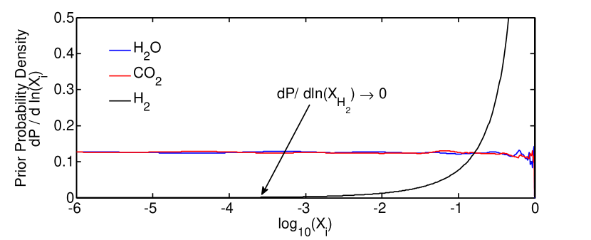
Previous work on atmospheric retrieval implicitly accounted for the constraints in Equations (7) and (8) by using free parameters only for mixing ratios of the minor atmospheric gases and assuming that the remainder of the atmosphere is filled with the a-priori known main constituent. This approach is feasible for the inference of gas mixing ratios in hot Jupiters and Solar System planets because the main constituents of the atmospheres, i.e., $\mbox{H}_{2}$, are known a priori. In a Bayesian retrieval approach, in which we do not know the main constituent of the atmosphere, however, parameterizing the abundances of minor species and assuming a main species is unfavorable. Assigning a Jeffrey prior, i.e. a uniform prior on the logarithmic scale, for $n-1$ mixing ratios leads to a highly asymmetric prior that favors a high abundance of the $n$th species (Figure 1 (top)). In addition, in cases with a low abundance of the $n$th species, we find that the asymmetric parameterization leads to serious convergence problems in the numerical posterior simulation with MCMC.

To circumvent the drawbacks of highly asymmetric priors in the interpretation of the results as well as the numerical convergence problems due a highly asymmetric parameterization, we use the centered-log-ratio transformation to reparameterize the composition (Aitchison, 1986; Pawlowsky-Glahn & Egozcue, 2006). The centered-log-ratio transformation is commonly used in geology and social sciences for the statistical analysis of compositional data (e.g., Pawlowsky-Glahn & Egozcue, 2006), we find that it also enables the MCMC technique to efficiently explore the posterior distribution of the atmospheric composition across the complete simplicial sample space.

For a mixture of $n$ gases, the centered-log-ratio transformation of the $i$-th molecular species is defined as

$$\xi_{i}=\mathrm{clr}\left(X_{i}\right)=\ln\frac{X_{i}}{g(\boldsymbol{x})},$$ (9)

where

$$g(\boldsymbol{x})=\left(\prod_{j=1}^{n}X_{i}\right)^{1/n}=\exp\left(\frac{1}{n}\sum_{j=1}^{n}\ln X_{i}\right)$$ (10)

is the geometric mean of all mixing ratios $X_{1}...X_{n}$.

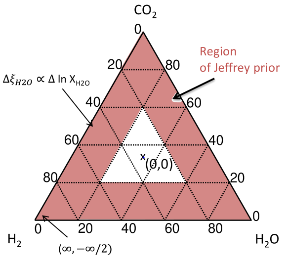
Each of the compositional parameters $\xi_{i}$ may range between $-\infty$ and $+\infty$, where the limit $\xi_{i}\rightarrow-\infty$ indicates that $i$th species is of extremely low abundance with respect to the other molecular species, while $\xi_{i}\rightarrow+\infty$ indicates that the $i$-th species is abundant in the atmosphere. The composition $\boldsymbol{\xi}=\left[0,0,\ldots,0\right]$describes the center of the simplex at which all molecular species are equally abundant (Figure 2). The only constraints on the transformed compositional parameters is $\sum_{i=1}^{n}\xi_{i}=0$.

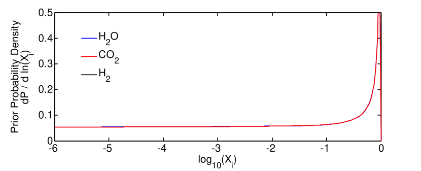
A fully permutation-invariant description is obtained by using the centered-log-ratio transformed mixing ratios $\xi_{1}\ldots\xi_{n-1}$ as the free parameters and assigning a uniform prior for all vectors in the $\mathbf{\xi}$-space for which $X_{i}>10^{-12}$ for all $i=1\ldots n$. As the distances in the sample space spanned by $\xi_{1}\ldots\xi_{n-1}$ scale with the differences in $\ln X_{i}$ for small mixing ratios, the MCMC can efficiently sample the complete space, even if the mixing ratios vary over several orders of magnitude.When transformed back into the Euclidean space of the mixing ratios, $X_{i}$, we obtain prior probabilities for each of the mixing ratios that have the properties of a Jeffrey prior below $X_{i}\lesssim 20\%$ (Figure 2). The properties of a Jeffrey prior are highly favorable for scale parameters such as the mixing ratios. The increase in the prior toward mixing ratios $\gtrsim 0.1$ is a direct consequence of the fact that one or more molecular species in the atmosphere inevitably needs to have a significant abundance. The divergence toward infinity at $\log X_{i}$ is of no practical relevance. If a single molecular species is detectable in the spectrum, then mixing ratios of 100% are excluded for all other species by the data .

Figure 1.— Marginalized prior probability distribution for the mixing ratios in a mixture of three gases. The upper panel illustrates the prior probabilities for a parameterization in which the gases $\mbox{H}_{2}\mbox{O}$ and $\mbox{CO}_{2}$ are described by free parameters and $\mbox{H}_{2}$ is set to fill the remainder of the atmosphere. Assigning a Jeffrey prior, i.e., $dP/d\ln\left(X_{i}\right)=\mathrm{const}$ to all gases except one leads to a description that is permutation variant and strongly favors compositions with a high abundance of the remaining gas. Compositions with low amount of $\mbox{H}_{2}$ are excluded by the prior because the prior probability rapidly approaches zero for $X_{\mbox{H}_{2}}<1\%$ . The bottom panel shows the prior probabilities for the mixing ratios using the center-log-ratio transformation introduced in this work. The prior probability for all gases in the mixture is identical, thereby providing permutation-invariant results. The prior probability distribution of all gases approaches the Jeffrey prior at mixing ratios below $\thicksim$20%, and is, therefore, highly favorable for scale parameters. The divergence to infinity is only of theoretical nature. Once the signature of one gas is detected in the spectrum, the posterior probability of all other gases at $X_{i}=100\%$ will go to zero.

Figure 2.— Simplicial sample space for a mixture of three gases illustrated in a ternary diagram. Using the centered-log-ratio transformation for the mixing ratios of the atmospheric gases, we obtain a symmetric parameterization of the composition in which all molecular species are treated equally, while simultaneously ensuring that the sum of the mixing ratios is unity. The zero point of the transformed mixing ratios, $\xi_{i}$, is at the center of the simplex. Toward the edges of the sample space, i.e., for low mixing ratios of one or more gases, the differences in the transformed mixing ratio, $\xi_{i}$, scale with $\ln\left(X_{i}\right)$. The scaling provides a region in which the prior probability $dP/d\ln(X_{i})$ remains constant (red) and allows the MCMC to efficiently sample down to exponentially small mixing ratios for all molecular species.

2.4. Inputs

The primary inputs to the retrieval method presented here are spectral and/or photometric observations of the wavelength dependent transit depths during the primary transit, $\left(R_{p}/R_{*}\right)^{2}$. Accurate estimates of the observational error bars are of particular importance because they can significantly affect the constraints and conclusions made from the observations. Ideally, the spectral data would not be binned to reduce the apparent error bars. Binning of spectral data always leads to a loss of information and should only be done if is required to compensate for systematics.

The spectra from the primary transit can be augmented by secondary eclipse measurements constraining the planetary albedo (or the atmospheric temperature) by including the information in the prior probability distribution. An improved estimate of the temperature or planetary albedo can lead to improved constraints in all composition parameters. If no such observations are available, the retrieved uncertainties in the composition will fully account for the uncertainty in the planetary albedo.

2.5. Outputs

The output of the atmospheric retrieval is the posterior probability density distribution, $p\text{$\left(\boldsymbol{x}|\boldsymbol{d}\right)$}$, of the retrieval parameters discussed in Section 2.1. This multidimensional distribution encodes our complete state of knowledge of the atmospheric parameters in the light of the available observations.. To illustrate our state of knowledge of a single parameter, we marginalize the posterior density distribution over all remaining parameters. For well-constrained parameters, one can summarize our knowledge of the parameter in just a few numbers, i.e., the most likely estimates and a set of error-bars and correlation coefficients. Depending on the nature of the observational data, however, we may obtain a posterior distribution that is not well-described by single best estimate plus the uncertainty around this estimate. For example, a multi-modal distribution would be indicative of multiple possible solutions. Highly asymmetric posterior distributions or only one-sided bounds will be obtained if the observations constrain the parameter only in one direction.

We can also compute the constraints on atmospheric properties that do not serve as free parameters in our retrieval methods, such as the mean molecular mass, the total atmospheric mass above the surface, the mixing ratios by mass, or the elemental abundances. A set of the retrieval parameters introduced in Section 2.1 entirely describes the state of well-mixed, one-dimensional atmospheres. For each set of retrieval parameters in the chain obtained from the MCMC simulations, we can, therefore, compute the any other atmospheric property from the retrieval parameters. In this way, we obtain a new chain for the desired atmospheric property that, interpreted as a sample from the marginalized distribution of the atmospheric property, can be used to infer constraints on the atmospheric properties by comparing the distribution to the equivalently obtained prior distribution.

In this work, we present constraints on the mean molecular mass, total atmospheric mass above the cloud-deck/surface, and relative elemental abundances (Equations 10-12),

$$\mu_{\mathrm{mix}}=\sum_{i=1}^{n}\mu_{i}X_{i}$$ (11)

$$M_{\mathrm{atm}}=\int 4\pi r^{2}\rho\left(r\right)dr$$ (12)

$$q_{j}=\frac{\sum_{i}^{n_{\mathrm{mol}}}X_{i}n_{i,j}}{\sum_{j}^{n_{\mathrm{elem}}}\sum_{i}^{n_{\mathrm{mol}}}X_{i}n_{i,j}}$$ (13)

where $q_{j}$ is the relative abundance of the elemental species $j$, $X_{i}$ is the mixing ratio of molecule $i$, and $n_{i,j}$ is the number of atoms of elemental species $j$ in molecule $i$.

3. Synthetic Observations of Super-Earth Transmission Spectra

The goal of the quantitative analysis presented in this work is to explore which constraints on the atmospheric properties of super-Earth exoplanets can be extracted from low-noise transmission spectra in the coming decades. In this section, we describe synthetic, low-noise observations of the transmission spectra of three different, hypothetical types of hot super-Earths transiting nearby M-stars as they may be obtained with the James Webb Space Telescope (JWST). To make the results most relevant in the context of current observational efforts, we adopt the stellar, orbital, and planetary parameters of the super-Earth GJ 1214b (Charbonneau et al., 2009).

3.1. Atmospheric Scenarios

“Hot Halley world.”

The first scenario we consider is a volatile-rich super-Earth (Kuchner, 2003; Léger et al., 2004). The motivation for this scenario is to investigate the retrieval results for an atmosphere that is predominately composed of absorbing gases. For our specific case, we consider a scenario in which the planet has accreted ices with the elemental abundances of the ices identical to those in the Halley comet in the Solar System (Jessberger & Kissel, 1991). Some of the ices may have evaporated at the high equilibrium temperature and formed an atmosphere around the planet. We assume a well-mixed atmosphere around the planet whose chemical composition is calculated from chemical equilibrium at the 1 bar level. The resulting atmosphere is composed of $\mathrm{H_{2}O}$ (69.5%), $\mathrm{CO_{2}}$ (13.9%), $\mathrm{H_{2}}$ (11.8%), $\mathrm{CH_{4}}$ (2.6%), and $\mathrm{N_{2}}$ (2.2%). All mixing ratios are givenas volume mixing ratios. The atmosphere is assumed to be clear and sufficiently thick such that no surface affects the transmission spectrum in this scenario. (Table 1).

“Hot nitrogen-rich world.”

For the second scenario we consider a nitrogen-dominated atmosphere representative of a rocky planet with an outgassed atmosphere similar to the atmospheres of Earth and Titan. The motivation for this scenario is to investigate the retrieval results for an atmosphere that is predominately composed of a spectrally-inactive gas that has no directly observable features in the spectrum. We chose an atmosphere dominated by $\mathrm{N_{2}}$ (95.4%) and rich in $\mathrm{CH_{4}}$ (3.5%), $\mathrm{CO_{2}}$ (1%) and $\mathrm{H_{2}O}$ (0.1% ) with a rocky surface at 1 bar.

“Hot mini-neptune.”

The third scenario is a super-Earth with a thick hydrogen/helium envelope that has experienced a formation history similar to those of the giant planets. While we assume a primordial atmosphere, we deliberately chose an example that is away from solar abundance and chemical equilibrium. The motivation for this scenario is to demonstrate the retrieval for a scenario that does not correspond to our preconceived ideas. The atmosphere we consider is composed of 84.9% $\mathrm{H_{2}}$, 13.1% $\mathrm{He}$, and 2% $\mathrm{H_{2}0}$, and has small mixing ratios of $\mathrm{CO_{2}}$ ($10^{-6})$ and $\mathrm{CH_{4}}$ ($10^{-7})$. We consider the presence of an opaque cloud deck of unknown nature at the 100 mbar level.

Planet Scenario	$X_{\mathrm{H_{2}O}}$	$X_{\mathrm{CO_{2}}}$	$X_{\mathrm{CH_{4}}}$	$X_{\mathrm{H_{2}}}$	$X_{\mathrm{He}}$	$X_{\mathrm{N_{2}}}$	Surface
Hot Halley world	69.5%	13.9%	2.6%	11.8%	$\approx 0$	2.2%	None
Hot nitrogen-rich world	0.1%	1%	3.5%	$\approx 0$	$\approx 0$	95.4%	Rocky surface at$1\,\mathrm{bar}$
Hot mini-neptune	2%	$10^{-6}$	$10^{-7}$	84.9%	13.1%	$\approx 0$	Cloud deck at $100\,\mathrm{mbar}$

Table 1Mixing Ratios Of Molecular Constituents and Surface Pressure for the Three Super-Earth Scenarios Used to Generate Synthetic Transmission Spectra.

3.2. Observation Scenarios

For each of the three atmospheric scenarios, we simulate high-resolution transmission spectra ($R>10^{5})$ and model the output of the JWST NIRSpec instrument covering the spectral range between $0.6$ and $5\,\mathrm{\mu m}$. We assume that the transit depths in the individual channels of JWST NIRSpec can be determined to within 20% of the shot noise limit. To compute the photon flux for each spectral channel individually, we scale the spectrum of a typical M4.5V star (Segura et al., 2005) to the apparent brightness of GJ 1214. For JWST, we adopt an effective diameter of the primary mirror of $6.5\,\mathrm{m}$ and a throughput before the instrument of 0.88 (Deming et al., 2009). We consider the spectral resolution for observations using the $R$=100 $\mbox{CaF}_{2}$ prism on NIRSpec ($R=30\ldots 280$). Our noise model adopts a total optical transmission for the NIRSpec optics after the slit of 0.4 and a quantum efficiency for the HgCdTe detector of 0.8 (Deming et al., 2009). We do not include any slit losses because the large aperture of JWST will encompass virtually all of the energy in the point source function. We find that read noise ($6\,e^{-}$per Fowler 8) and dark current ($0.03\,\mathrm{e^{-}\,s^{-1}}$) are insignificant compared to photon noise. We account for a $\sim 20\%$ loss of integration time due to the resetting and reading-out of the detector, based on the expected saturation time of 0.43 sec for the brightest pixels on the NIRSpec detector for GJ 1214 (de Wit, personal communication). For a first order estimate of the observational errors, we neglect the wavelength dependence of the grating blaze function.

Given the instrument properties, we calculate the expected variances of the in-transit and out-of-transit fluxes due to shot noise and calculate the expected error in the observed transit depth. We assume that the total observation time used to measure the baseline flux before and after the transit equals the transit duration. We stack 10 synthetic transit observations for the high mean molecular mass atmospheres of the "hot Halley world" and "hot nitrogen-rich world" scenarios and use only a single transit observation for the more easily detectable hydrogen-dominated "hot mini-neptune" scenario.

4. Results

Our most significant finding is that a unique constraint on the mixing ratios of the absorbing gases and up to two spectrally inactive gases is possible with moderate-resolution transmission spectra. Assuming a well-mixed atmosphere and that $\mathrm{N}_{2}$ and a primordial mix of $\mathrm{H_{2}+He}$ are the only significant spectrally inactive components, we can fully constrain the molecular composition of the atmosphere. We also find, however, that even a robust detection of a molecular absorption feature (>10$\sigma$) can be insufficient to determine whether a particular absorber is the main constituent of the atmosphere ($X_{i}>50\%$) or just a minor species with a mixing ratio of only a less than 0.1%, if we do not observe the signature of gaseous Rayleigh scattering.

In this section, we first conceptually identify the features in the spectrum that are required to uniquely constrain the compositions of general exoplanet atmospheres (Section 4.1). Based on the conceptual understanding, we then present numerical results from the MCMC retrieval analysis for synthetic JWST NIRSpec observations of three scenarios for the super-Earth GJ 1214b (Section 4.2).

4.1. Uniquely Constraining Exoplanet Atmospheres

Identifying absorbing molecules by their spectral features is conceptually straightforward, as molecules generally absorb at distinct wavelengths. Constraining the mixing ratios of the atmospheric gases is more complicated because the observable transmission spectrum depends not only on the mixing ratios of the absorbers, but also on the exact planetary radius (as measured by the radius at the reference pressure level, $R_{P,10}$), the surface or cloud-top pressure, and the mean molecular mass of the background atmosphere. The absorber mixing ratios may therefore remain unconstrained over several orders of magnitude despite strong detections of a molecular absorption features in the near-infrared wavelength range. The difficulty in constraining the mixing ratios of the atmospheric constituents was not discovered in previous work on atmospheric retrieval because hot Jupiters were assumed to be cloud-free and the mean molecular mass of their hydrogen-dominated atmospheres was known a priori (e.g., Madhusudhan & Seager, 2009). In the following, we explain which observables from different parts of the spectrum must be combined to successfully constrain the composition of a general exoplanet atmosphere.

The transmission spectrum of an atmosphere with $n$ relevant absorbers provides $n+4$ independent observables (Figure 3). Combined, these $n+4$ observables can be used to constrain the $n$ unknown mixing ratios of the absorbing gases, the mixing ratios of up to two spectrally inactive gases (e.g., $\mbox{N}_{2}$ and primordial $\mbox{H}_{2}+\mbox{He}$), the planetary radius at reference pressure level, and the pressure at the surface or upper cloud deck. The remaining information in the transmission spectrum is highly redundant with the $n+4$ independent observables.

Figure 3.— Unique constraints on the atmospheric properties based on observables in the transmission spectrum. The transmission spectrum of an atmosphere with $n$ relevant absorbers contains $n+4$ independent pieces of information that constrain the $n$ mixing ratios of these absorbers, up to two mixing ratios of the two spectrally inactive components $\mbox{H}_{2}+\mbox{He}$ and $\mbox{N}_{2}$, the planetary radius at a reference pressure level, $R_{P,10}$, and the surface/cloud-top pressure. The left panel illustrates conceptually the individual observables in the transmission spectrum that carry the $n$+4 pieces of information for an example with $n=3$ absorbers. For well-mixed atmospheres, the three observables “Slope of the Rayleigh signature,”, “Shapes of individual features,” and “Relative transit depths in features of same molecule” are redundant and provide only one independent piece of information. Note that to uniquely constrain any of the $n+4$ atmospheric properties on the far right, all $n+4$ pieces of information need to be available, unless additional assumptions are made.

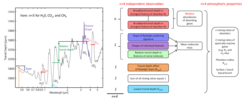
The $n+4$ independent observables are as follows. For each of the $n$ absorbers, the broadband transit depths in the strongest features provide one independent observable. By measuring and comparing the broadband transit depths in the absorption features of different molecules, we can directly determine the relative abundances of the absorbing gases in the atmosphere (Section 4.1.1). For example, given the broadband transit depths in the 3.3 µm $\mbox{CH}_{4}$ feature and in the 4.3 µm $\mbox{CO}_{2}$ feature, we can determine that there must be “x” times more $\mbox{CO}_{2}$ than $\mbox{CH}_{4}$ in the atmosphere. If the feature of one molecular absorber is not present, transit depth measurements at wavelengths for which the absorption cross sections of the molecular species are high can still provide an upper limit on the absorber abundance relative to the other absorbers.

Next, we have a total of one additional piece of information from either (1) the linear slope of the Rayleigh signature, (2) the shapes of individual features, or (3) the relative transit depths in features of the same molecule. The information from the three observables is highly redundant. From one of the three observables, we can directly constrain the scale height, and, given an approximate estimate of the atmospheric temperature, we can obtain an estimate of the mean molecular mass (Section 4.1.2). Importantly, for general atmospheres that may contain clouds, it is the slope at which the transit depth changes as a function of the extinction cross section thatenables us to measure the mean molecular mass. The overall transit depth variation as currently discussed in many papers on the super-Earth GJ 1214b (e.g., Miller-Ricci & Fortney, 2010; Bean et al., 2011; Croll et al., 2011) measures the mean molecular mass only for cloud-free atmospheres.

Three additional independent constraints are provided by the transit depth offset of the Rayleigh slope, the fact that all mixing ratios must sum to 1, and the measure of the lowest transit depths in the spectrum. Comparing the transit depth offset of the Rayleigh slope and the transit depths at near-infrared wavelengths provides us with a measure of the amount of spectrally inactive gas in the atmosphere. Given all previously discussed observables, the lowest transit depths in the spectrum allow us to independently constrain the surface/cloud-top pressure (Section 4.1.4). If the surface/cloud-top is at a deep layer in the atmosphere and the molecular opacities across the observed wavelength range are high, a direct detection of a surface is not possible. In this case, the minimum transit depth will provide a lower limit on the surface/cloud-top pressure.

Note that we need all $n+4$ observables together in order to determine any of the atmospheric parameters uniquely. If a single piece of the puzzle is missing, e.g., the transit depths at short wavelengths are not observed, then the composition, including the volume mixing ratios of the absorbers, will stay weakly constrained, even if we have detected the feature with high significance.

4.1.1 Relative Abundances of Absorbing Gases

?figurename? 4.— Degeneracy between the absorber mixing ratio, $X_{\mathrm{CO_{2}}}$, and the planetary radius at the reference pressure level, $R_{P,10}$. The left panel illustrates the modeled transmission spectra in the $4.3\mathrm{\mu m}$ $\mathrm{CO_{2}}$ absorption feature for two different atmospheric compositions. The atmospheric composition of scenario 1 (red) is 10% $\mathrm{CO_{2}}$ and 90% $\mathrm{N_{2}}$. For the same planetary radius, the transit depth in the absorption feature of scenario 2 (blue; 0.1% $\mathrm{CO_{2}}$ and 99.9% $\mathrm{N_{2}}$) is lower by $\mathrm{\sim 100\,ppm}$ across the entire feature. Increasing the planetary radius for scenario 2, however, leads to a transmission spectrum (green) that closely resembles scenario 1. As a result of this degeneracy between $X_{\mathrm{CO_{2}}}$ and $R_{P,10}$, the mixing ratio of $\mathrm{CO_{2}}$ cannot be determined to within several orders of magnitude even for low-noise observations of the feature. The right panel shows the total pressures for planets with two different planetary radii (black) and the partial pressure of C$O_{2}$ as a function of the distance from the planetary center (colors match left panel). Two atmospheres with different absorber mixing ratios (red and green) can have the same partial pressure/number density as function of distance from the planetary center leading to similar absorption features.

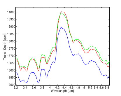
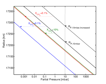
The infrared part of the transmission spectrum provides a good tool to constrain the relative abundances of the molecular absorbers. Constraining the absolute value of the volume mixing ratios, however, might not be possible to within orders of magnitude, even with low-noise observations capturing the shapes of the absorption features because the infrared part of the spectrum lacks an absolute reference for the transit depth.

The measured transit depths in the absorption features are mainly related to the number density of the absorbing molecule, $n_{i}\left(r\right)$, as a function of the radius from center of the planet, $r$. The function $n_{i}\left(r\right)$, however, provides little useful insight unless we are able to determine a surface radius or the number density of a second gas for comparison. In other words, if we do not detect a surface, then only the mixing ratios of the atmospheric gases have a meaningful interpretation, not the absolute number densities, because we are missing an absolute pressure scale. Obtaining the mixing ratios of an absorbing gas directly by observing the absorption features of this gas is complicated, however, because different combinations of the absorber mixing ratio, $X_{i}$, and the planetary radius, $R_{P,10}$, can lead to the same number density, $n_{i}\left(r\right)$, and, therefore, to virtually the same absorption feature shape. To constrain the mixing ratio of a particular gas independently, a reference for the planetary radius needs to be obtained from a different part of the spectrum.

Figure 5.— Constraining the relative abundances of absorbing gases from the near-infrared spectrum. The left panel shows the transmission spectrum for the atmospheric scenarios 1 (red, 10% $\mathrm{CO_{2}}$) and 2 (blue, 0.1% $\mathrm{CO_{2}}$) as described in Figure 4, but with 1% $\mbox{N}_{2}$ replaced by the absorbing gas $\mathrm{CH_{4}}$. While the $\mathrm{CO_{2}}$ features have a vertical offset between scenario 1 and scenario 2, the $\mathrm{CH_{4}}$ features are unaffected by the $\mathrm{CO_{2}}$ mixing ratio. The transit depth in $\mbox{CH}_{4}$ features can, therefore, serve as a relative reference for the $\mathrm{CO_{2}}$ mixing ratio. The right panel shows the two-dimensional marginal posterior probability distribution of the mixing ratios, $X\mathrm{{}_{CO_{2}}}$ and $X\mathrm{{}_{CH_{4}}}$ as retrieved from low-noise synthetic observations of the near-infrared spectrum ($R$=100, $\sigma_{\left(Rp/R*\right)^{2}}\thickapprox 20\,\mbox{ppm},$ $\lambda=2\textrm{-}5\,\mbox{$\mu$m}$) of scenario 1. The solid lines indicate the 1$\sigma$, 2$\sigma$, and 3$\sigma$ credible regions. Measuring the transit depth in infrared features of $\mathrm{CO_{2}}$ and $\mathrm{CH_{4}}$ provides good constraints on the relative abundance ratios of the two gases. The volume mixing ratios of the gases, however, are strongly correlated. The individual mixing ratios remain unconstrained across three orders of magnitude despite robust detections of the infrared features and sufficient spectral resolution to observe the feature shapes.

For a quantitative example, we show the $4.3\,\mathrm{\mu m}$ absorption feature of $\mathrm{CO_{2}}$ for two different atmospheric compositions in Figure 4. The compositions are 90% $\mathrm{N_{2}}$ and 10% $\mathrm{CO_{2}}$ for scenario 1 and 99.9% $\mathrm{N_{2}}$ and 0.1% $\mathrm{CO_{2}}$ for scenario 2. If the planetary radius, $R_{P,10}$, for the two scenarios is the same, more starlight is blocked in scenario 1 due to the higher number density $n_{\mathrm{CO_{2}}}\left(r\right)$. The transit depth inside the spectral features of $\mathrm{CO_{2}}$ is therefore higher than for scenario 2. If the planetary radius $R_{P,10}$ in scenario 2 is increased by only 70 km ($\approx 0.4\%$ ), however, then the number density $n_{\mathrm{CO_{2}}}\left(r\right)$ in scenarios 2 equals the one in scenario 1, and the absorption feature of scenario 1 closely resembles the absorption feature of the new scenario 2. The remaining small difference in the transmission spectra is due to the effect of pressure and temperature on the absorption line broadening. The effect of changes in line broadening is of secondary order though, which makes the distinction between scenarios 1 and 2 difficult, even with extremely low-noise observations. Determining the mixing ratio of $\mathrm{CO_{2}}$ by observing only $\mathrm{CO_{2}}$ features is, therefore, highly impractical.

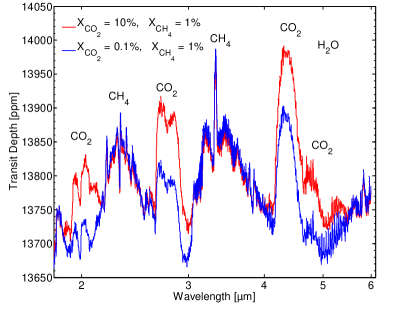
A relative reference to break the degeneracy between the planetary radius and the mixing ratio is provided by the transit depths in absorption features of different absorbers. Conceptually, this is possible because a change in the planetary radius affects the absorption features of both gases equally, while a change in the mixing ratio of one of the absorbers only affects the features of that absorber. The transit depth difference between two features of different absorbers is independent of the planetary radius and only dependent on the relative abundance ratios of the absorbers and their absorption cross sections in the features. As the absorption cross section are known from the molecular databases, comparing the transit depths in features of different absorbers allows one to constrain the relative abundance of these absorbers. For a numerical example, we return to our $\mathrm{N}_{2}$-$\mbox{CO}_{2}$ atmosphere and replace 1% $\mbox{N}_{2}$ by $\mathrm{CH_{4}}$. In the spectral region around the $3.5\,\mathrm{\mu m}$ $\mathrm{CH_{4}}$ feature (Figure 5), the spectrum remains unaffected by the change in the $\mathrm{CO_{2}}$ mixing ratio and can serve as a reference to probe the relative abundances of $\mbox{CO}_{2}$ and $\mbox{CH}_{4}$.

The infrared part of the transmission spectrum covering multiple absorption features of different molecular species, therefore, provides good constraints on the relative abundances of the molecular absorbers, but hardly contains any information on the volume mixing ratios of the absorbers. Even low-noise NIR observations capturing the shapes of the absorption features might not constrain the absolute value of the mixing ratio to within orders of magnitude because the infrared part of the spectrum provides little information on the abundances of spectrally inactive gases.

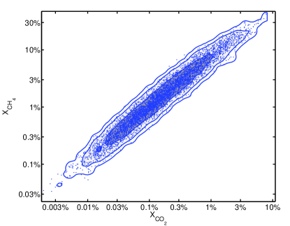
In our example, the abundance ratio $\frac{X_{\mathrm{CH_{4}}}}{X_{\mathrm{CO_{2}}}}$is constrained to within a factor of a few at 3$\sigma$, while the volume mixing ratio of $\mathrm{CH_{4}}$ compatible with the simulated observation can vary over three orders of magnitude between 0.03% and 30%. Note that the reason for the correlation between $X_{CO_{2}}$and $X_{CH_{4}}$ is not the overlap of absorption features of the molecular species. Overlapping features would cause an anti-correlation between the abundances of the two absorbers.

4.1.2 Mean Molecular Mass

It has been shown that, for clear atmospheres, measuring the change in transit depth, $\Delta D$, across spectral features gives an order of magnitude estimate of the scale height and, therefore, the mean molecular mass (Miller-Ricci et al., 2009). For a general atmosphere, however, the depth of the absorption features cannot be used to constrain the mean molecular mass because clouds, hazes, and a potentially present surface also affect the depths of spectral features. Here we show for general atmospheres that the value of the mean molecular mass can be determined by measuring the slope, $\frac{dR_{P,\lambda}}{d\left(ln\sigma_{\lambda}\right)}$ , with which the "observed" planet radius, $R_{P,\lambda}$, changes as a function of the extinction cross section, $\sigma_{\lambda}$, across different wavelengths. In practice, good observables to independently constrain the mean molecular mass are (1) the slope Rayleigh scattering signature at short wavelengths, (2) the relative sizes of strong and weak absorption features of the same molecule, and (3) the shape of the wings of a strong molecular absorption feature.

For the optically thick part of the spectrum, the observed radius of the planet changes linearly with the logarithm of the extinction cross section (Etangs et al., 2008) and the slope $\frac{dR_{P,\lambda}}{d\text{$\left(ln\sigma_{\lambda}\right)$}}$ is directly related to the atmospheric scale height,

$$H=\frac{dR_{P,\lambda}}{d\text{$\left(\ln\sigma_{\lambda}\right)$}}.$$ (14)

A measurement of the observed planet radius, $R_{P,\lambda}$, at two or more wavelengths with different absorption or scattering cross sections, $\sigma_{\lambda}$, therefore, permits the determination of the scale height. Given an estimate of the atmospheric temperature, e.g. $T\approx T_{eq}$, we can observationally determine an estimate of the mean molecular mass

$$\mu_{\mathrm{mix}}=\frac{k_{B}T}{g}\left(\frac{dR_{p,\lambda}}{d\text{$\left(\ln\sigma_{\lambda}\right)$}}\right)^{-1}\times\left(1\pm\frac{\delta T}{T}\right),$$ (15)

where the factor $\left(1\pm\frac{\delta T}{T}\right)$ accounts for the inherent uncertainty due to the uncertainty, $\delta T$, in modeling the atmospheric temperature, $T$, at the planetary radius $r=R_{P,\lambda}$ (Appendix). Even if the uncertainty in the temperature estimate is several tens of percents of the face value, we will find useful constraints on the mean molecular mass because the mean molecular mass varies by a factor on the order of $8-20$ between hydrogen-dominated atmospheres and atmospheres mainly composed of $H_{2}$O, $N_{2}$, or C$O_{2}$.

The most straightforward way to determine the mean molecular mass is to measure the slope of the Rayleigh scattering signature at short wavelengths. The Rayleigh scattering coefficient varies strongly with wavelength as $\sigma\left(\lambda\right)\varpropto\lambda^{-4}$ . From $\sigma\left(\lambda\right)\varpropto\lambda^{-4}$, we obtain

$$\mu_{mix}=\frac{4k_{B}T}{gR_{*}}\frac{\ln\left(\frac{\lambda_{1}}{\lambda_{2}}\right)}{\left(\frac{R_{p}}{R_{*}}\right)_{\lambda_{2}}-\left(\frac{R_{p}}{R_{*}}\right)_{\lambda_{1}}}\times\left(1\pm\frac{\delta T}{T}\right),$$ (16)

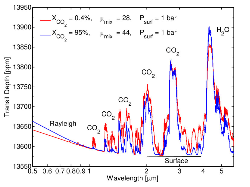
Measuring the transit depth $D_{\lambda}=\left(\frac{R_{p}}{R_{*}}\right)_{\lambda}^{2}$ at two different wavelengths $\lambda_{1}$ and $\lambda_{2}$ that are dominated by Rayleigh scattering, therefore, provides the mean molecular mass. For a quantitative example, we show the transmission spectra of a $\mathrm{CO_{2}}$-dominated atmosphere (95% $\mathrm{CO_{2}}$+ 5% $\mathrm{N_{2}})$ and a $\mathrm{N_{2}}$-dominated atmosphere with small amount of $\mathrm{CO_{2}}$ as the only absorber (0.15% $\mathrm{CO_{2}}$, 99.85% $\mathrm{N_{2}}$) in Figure 6. Despite the difference in mean molecular mass, the feature depths are similar due to the different total amounts of the absorber $\mathrm{CO_{2}}$; thus, the feature depth cannot be used to determine the scale height. The Rayleigh slope at short wavelength ($\lambda<0.8\mu\mathrm{m}$), however, is only affected by the scale height and can serve as a good measure of the mean molecular mass.

A second way of constraining the mean molecular mass is based on analyzing the detailed shape of the wing and core of spectral features. The absorption cross section varies strongly from the center to the outer wings. Measuring the detailed shape of a spectral feature at sufficient spectral resolution, therefore, probes a large range of cross sections and allows the constraint of the mean molecular mass. In our example, the detailed shape of the $4.3\,\mu\mbox{m}$ $\mathrm{CO_{2}}$ feature shows the difference between the scenarios (Figure 6). For smaller mean molecular mass, the feature is higher at the center with narrow wings, while the large mean molecular mass leads to broader features. The measurement of this difference requires at least a moderate spectral resolution ($R\sim 50$) and a high signal-to-noise ratio (S/N).

A third way to probe the mean molecular mass is to quantitatively compare the broadband transit depths in different spectral features of the same absorber. Again, we probe the planetary radius at wavelengths for which the cross sections are different: strong absorption features have large absorption cross sections, while weaker features of the same absorber have smaller cross sections. A quantitative comparison of the depths of individual features therefore provides the gradient $\frac{dR_{P,\lambda}}{d\text{$\left(ln\sigma_{\lambda}\right)$}}$ and constrains the scale height and mean molecular mass. For atmospheres with small mean molecular masses, the gradient $\frac{dR_{P,\lambda}}{d\text{$\left(ln\sigma_{\lambda}\right)$}}$ is large, resulting in greater differences in the transit depths between the strong and the weak features (Figure 6).

?figurename? 6.— Visible to near-infrared transmission spectra for two atmospheric scenarios with similar absorption feature sizes. The first scenario (blue) is a $\mathrm{N_{2}}$-rich atmosphere (0.15% $\mathrm{CO_{2}}$, 99.85% $\mathrm{N_{2}}$). The second scenario (red) is $\mbox{CO}_{2}$ dominated (95% $\mathrm{CO_{2}}$ and 5% $\mathrm{N_{2}}$). Despite the different mean molecular mass (28 vs. 44) the infrared absorption feature sizes are similar because the difference in the vertical extent of the atmosphere due to the different scale heights is compensated for by the difference in the total amount of the absorbing $\mathrm{CO_{2}}$ gas. A reliable way to determine the scale height is to measure either the Rayleigh scattering slope $\frac{dR_{P,\lambda}}{d\text{$\left(\ln\lambda\right)$}}$ at short wavelengths, the slope $\frac{dR_{P,\lambda}}{d\text{$\left(ln\sigma_{\lambda}\right)$}}$ in strong absorption features, or the relative feature depths between strong and weak features of the same molecule. The lower mean molecular mass atmosphere (blue) shows a steeper Rayleigh scattering slope, larger differences in the $\mbox{CO}_{2}$ absorption features depth, and narrower features than the higher mean molecular mass atmosphere (red).

4.1.3 Volume Mixing Ratios of the Atmospheric Constituents

The primary quantities affected by the abundance of spectrally inactive gases are the estimate of the mean molecular mass, $\mu_{\mathrm{mix}}$, discussed in Section 4.1.2 and the transit depth offset of the molecular Rayleigh scattering slope, $D_{\mathrm{Rayl}}$. Combining the information on $\mu_{\mathrm{mix}}$ and $D_{\mathrm{Rayl}}$ with the constraints on the relative abundances of the absorbers from the NIR spectrum (Section 4.1.1) provides unique constraints on the volume mixing ratios of both the spectrally inactive gases and molecular absorbers.

The atmospheres of Jupiter-sized planets present a simplified case for atmospheric retrieval. From their radius and mass measurements, we can conclude that they have accreted a hydrogen-dominated atmosphere, thus we know the mean molecular mass a priori. Constraining the volume mixing ratios of the molecular species in the atmosphere, nonetheless, requires the observation of the transit depth offset of the molecular Rayleigh scattering slope, $D_{\mathrm{Rayl}}$ at short wavelength.

Neglecting for now the effect of refractive index variations between different gas mixtures, the transit depth offset of the molecular Rayleigh scattering slope, $D_{\mathrm{Rayl}}$, is only a function of planetary radius at the reference pressure, $R_{P,10}$. The transit depth offset of the Rayleigh scattering signature can, therefore, serve as a reference transit depth to obtain an absolute scale for the atmospheric pressure and to determinethe volume mixing ratios of the absorbers from the absorption features in the NIR. In general, atmospheres rich in absorbing gases will show transmission spectra for which the transit depth in the Rayleigh scattering signature is small with respect to the transit depth in the NIR, while atmospheres dominated by spectrally inactive gases will show transmission spectra that have a strong Rayleigh scattering signatures and absorption features in the NIR at a lower transit depth levels.

Obtaining the absolute abundances for all relevant absorbing gases enables us to constrain the total mixing ratio of the spectrally inactive gases to be $X_{\mathrm{inactive}}=1-\sum_{i=1}^{n}X_{i}$, where $n$ is the number of absorbers in the atmosphere. Conceptually, the estimate of the mean molecular mass, $\mu_{\mathrm{mix}}$, can then be used to determine the individual mixing ratios of the spectrally inactive components, $\mbox{N}_{2}$ and $\mbox{H}_{2}+\mbox{He}$. We obtain the volume mixing ratios of $\mathrm{N}_{2}$ and primordial gas from

$$\mu_{mix}=\mu_{N_{2}}X_{N_{2}}+\mu_{H_{2}+He}\left(X_{inactive}-X_{N_{2}}\right)+\sum_{i=1}^{n}\mu_{i}X_{i}$$ (17)

and

$$X_{\mathrm{H_{2}+He}}=X_{\mathrm{inactive}}-X_{\mathrm{N_{2}}}.$$ (18)

Individual constraints on $\mbox{H}_{2}$ and He are not possible because only two spectrally inactive gases can be fit. Three or more individual spectrally inactive components inherently lead to degeneracy because the same mean molecular mass of the spectrally inactive gases can be obtained by different combinations of the mixing ratios of the gases.

In reality, the effective refractive index of the gas mixture varies depending on the composition and affects the transit depth offset of the Rayleigh scattering signature (Section 2.2.1). When simultaneously retrieving the mixing ratios of all gases, however, we also determine the refractive index in the process because the refractive index is a direct function of only the mixing ratios and not an additional unknown.

4.1.4 Surface Pressure

We can discriminate between a thick, cloud-free atmosphere and an atmosphere with a surface, where the surface is either the ground or an opaque cloud deck. For atmospheres with an upper surface at pressures lower than $P_{\mathrm{surf}}\lesssim\mathrm{100\,mbar\ldots 5\,bar}$ (depending on composition), we can quantitatively constrain the pressure at this surface. For a thick atmosphere, we can identify a lower limit on the surface pressure.

A surface strongly affects the part of the spectrum without absorption features while having only a weak or negligible effect on the part of the transmission spectrum with strong molecular absorption or scattering. In the spectral regions with weak absorption, a thin atmosphere has a relatively constant continuum because the surface cuts off the grazing light beams at a radius that is independent of the wavelength (Des Marais et al., 2002; Ehrenreich et al., 2006). A thick atmosphere without a surface lacks a flat continuum.

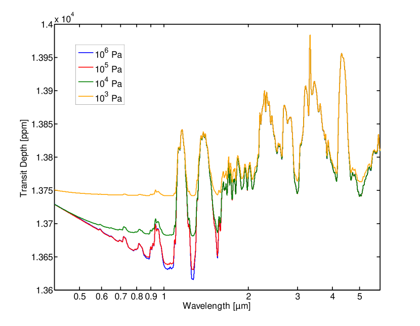
Conceptually, the optically-thick regions of the spectrum, those for which the transit depth is independent of the surface pressure, constrain the mixing ratios of the molecular species in the atmosphere as described in Section 4.1. The surface pressure can then be determined from the transit depths in the parts of the spectrum in which absorption and scattering are weak (Figure 3). For a noise-free spectrum, the strongest constraint on the surface pressure is provided by the minimum transit depth, $D_{\mathrm{min}}$, measured across the spectrum. The minimum transit depth determines the deepest pressure level for which light is transmitted through the atmosphere and, therefore, provides a lower limit on the surface pressure. In practice, the retrieval of the mixing ratios, surface pressure, and other parameters is performed simultaneously based on the information in the entire spectrum.

Taking the example of a $\mathrm{N_{2}}$-$\mathrm{CO_{2}}$ atmosphere (Figure 7), the shape of the spectral features in the 2-6 $\mathrm{\mu m}$ range is mostly unaffected by changes in surface pressure, as long as the surface pressure is higher than $100\,\mathrm{mbar}$. For exquisite data, the composition of the atmosphere can, therefore, be retrieved from the 2 to $\mathrm{6\,\mu m}$ range independently of the surface pressure. Conversely, the spectral region between 0.5 and 2 $\mathrm{\mu m}$ is strongly affected by surface pressure, but the effects of surface pressure and mixing ratios are usually degenerate. Taking the retrieved mixing ratios from the part of the spectrum unaffected by surface pressure, allows a unique determination of the surface pressure.

?figurename? 7.— Effect of the surface pressure on the transmission spectra of exoplanets. The transmission spectra of model atmospheres with 99% $\mathrm{N_{2}}$ and 1%$\mathrm{CO_{2}}$ are depicted for four different surface pressures. The radius, $R_{P,10}$, at which the atmospheric pressure is 10 mbar is set to the same value for all four. With $R_{P,10}$ set to the same value, the transit depths in the strong $\mathrm{CO_{2}}$ absorption bands (e.g., around 2.7, 3.3, and 4.3$\mathrm{\mu m}$) are independent of the surface pressure since the grazing star light at these wavelengths does not penetrate to lower layers of the atmosphere. Conversely, the parts of the spectrum ($<1.6\,\mu\mathrm{m}$) with little molecular absorption and scattering show a strong dependence on the surface pressure. Combining information from parts of the spectrum that are sensitive to surface pressure and parts of the spectrum that are insensitive to surface pressure enables one to find independent constraints on atmospheric composition and surface pressure. At sufficiently high surface pressures, even the spectral regions with low absorption cross sections become optically thick for a grazing light beam and the complete spectrum becomes insensitive to further increases in the surface pressure. For these thick atmospheres, only a lower limit on the surface pressure can be found.

4.2. Numerical Results

4.2.1 Constraints on Composition

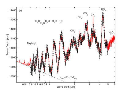
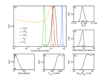
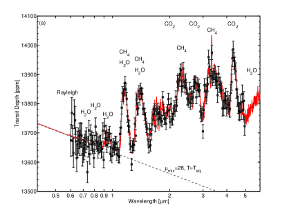
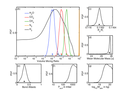
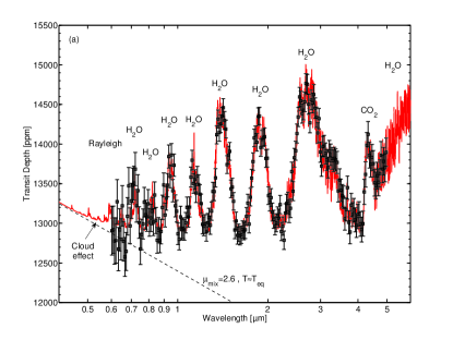
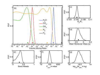
In this section, we present numerical results for synthetic JWST NIRSpec observations of the transmission spectrum of the super-Earth GJ 1214b. In all three atmospheric scenarios studied, we find that the analysis of moderate spectral resolution ($R\thickapprox 100)$ transmission spectra covering the spectral range between $0.6$ and $5\,\mu\mbox{m}$ can provide narrow probability posterior distributions for all absorbing gases with mixing ratios of several ppm or higher. (Figures 8-10). The well-constrained probability distributions allow a direct inference of the most likely estimate and credible regions (Bayesian equivalent to confidence intervals) for the mixing ratios of the individual molecular species. Spectrally inactive gases can also be constrained if their abundances are sufficient to affect the mean molecular mass and the Rayleigh scattering signature at short wavelengths.

For a given transmission spectrum, the relative uncertainties in the mixing ratios $\frac{\Delta X_{i}}{X_{i}}$ of absorbing gases (e.g., $\mathrm{H_{2}O},$ $\mathrm{CO_{2}}$, $\mathrm{CH_{4}}$) are only weakly dependent on the absolute values of the mixing ratios. In other words, minor gases with mixing ratios as low as tens of ppm can be constrained as well as the major atmospheric constituents (e.g., Figure 9(a)). The reason for this is that the long geometric path length of the grazing stellar light through the atmosphere of the extrasolar planet leads to significant spectral features in the transmission spectrum even for low-abundance gases (Brown, 2001). Increasing the mixing ratio increases the transit depth across the feature, but the uncertainty in the observed transit depth and, therefore, the uncertainty on the logarithm of the mixing ratio remains mostly unchanged. A detection limit does exist at low abundances, however because overlapping features of other absorbers may mask the features of extremely low-abundance gases. If all spectral regions in which the absorber is active are occupied by stronger features of other absorbers, then only an upper limit on the mixing ratio of the gas can be found (Figure 10).

In constrast to the absorbing gases, the uncertainties in the mixing ratios of spectrally inactive gases (e.g., $\mathrm{N_{2}}$, $\mathrm{H_{2}}$) are strongly dependent on their mixing ratios. Spectrally inactive gases affect the transmission spectrum only through changing the mean molecular mass and changing the transit depth difference between the Rayleigh scattering signature and the NIR spectrum (Section 4.1.3). If the mixing ratio of a spectrally inactive gas is a few tens of percent or more, the effect of the spectrally inactive gas on the atmospheric mean molecular mass is strong and, therefore, it is relatively easy to identify the spectrally inactive gas and constrain its mixing ratio (Figures 9 and 10). For lower mixing ratios, however, only weak constraints or an upper limit can be placed on the mixing ratios of spectrally inactive gases because their effect on the spectrum becomes negligible (e.g., Figure 8). This is particularly true for $\mathrm{N_{2}}$ whose molecular mass (28 u) differs only by a factor of $\sim 1.6$ or less from the molecular masses of the most common spectrally active gases, e.g., $\mathrm{H_{2}O}$ (18 u), $\mathrm{CH_{4}}$ (18 u), and $\mathrm{CO_{2}}$ (44 u). Constraining the mixing ratio of $\mathrm{H_{2}}$ is achieved down to lower mixing ratios because its molecular mass is lower than that of most absorbing gases by a factor of six or more.

4.2.2 Constraints on Surface Pressure

In the retrieval output, a thin atmosphere with a surface and a thick, cloud-free atmosphere show distinct posterior probability distributions for the surface pressure parameters. For atmospheres that are thin or have an upper cloud deck at low pressure levels, the probability distribution resembles a well-constrained, single-modal distribution (Figure 10(d)). For thick atmospheres that lack an observable surface, only an upper limit to the surface pressure can be retrieved (Figure 8(d))The posterior probability of the surface pressure plateaus toward high pressures, indicating that further increases in surface pressure lead to equally likely scenarios. We emphasize that, for a terrestrial planet, the two scenarios of a thin atmosphere with a solid surface or a thick atmosphere with an opaque cloud deck are not distinguishable from the transmission spectrum.

?figurename? 8.— Synthetic transit observations and atmospheric retrieval results for the "Hot Halley world" scenario for the super-Earth GJ 1214b. The synthetic observations shown in panel (a) were simulated considering 10 transit observations with JWST NIRSpec and assuming that observational uncertainties within 20% of the shot noise limit are achieved (see Section 3.2). The dashed line shows the analytical Rayleigh scattering slope for comparison. Panels (b)-(g) illustrate the marginalized posterior probability distribution for the atmospheric parameters retrieved from the synthetic observations. For illustrative purposes, the distributions are normalized to a maximum value of 1. The asterisks indicate the values of the atmospheric parameters used to simulate the input spectrum. The narrow, single-peaked, posterior probabilities for the mixing ratios of $\mathrm{H_{2}O,}$ $\mathrm{CO_{2}}$, $\mathrm{CH_{4}}$, and $\mbox{H}_{2}$ in panel (b) indicate that unique constraints on the abundance of these gases can be retrieved in agreement with the atmospheric parameters used to simulate the input spectrum. $\mathrm{H_{2}O}$ can be identified as the main constituent. Only an upper limit on the mixing ratio of $\mbox{N}_{2}$ can be found because small amounts of the spectrally inactive $\mbox{N}_{2}$ have a negligible effect on the observed transmission spectrum. Constraints are also obtained for the surface/cloud-top pressure and total atmospheric mass above the surface/cloud-top (Panels (f) and (g)). In this scenario, the atmosphere is cloud-free down to high pressure levels, thus only a lower bound on the surface pressure can be found. No upper bound can be inferred as indicated by the posterior probability distributions approaching the flat prior distribution at high surface pressures.

?figurename? 9.— Synthetic transit observations and atmospheric retrieval results for the "Hot nitrogen-rich world" scenario of a super-Earth with the physical properties of GJ 1214b. The panels identities are identical to Figure 8. Observational errors were modeled for 10 transit observations with JWST. The narrow posterior distributions for the mixing ratios of $\mathrm{H_{2}O,}$ $\mathrm{CO_{2}}$, $\mathrm{CH_{4}}$, and $\mbox{N}_{2}$ indicate that unique constraints on the abundance of these gases can be retrieved in agreement with the atmospheric parameters used to simulate the input spectrum. $\mathrm{N_{2}}$ can be identified to be the main constituent of the atmosphere due to its effect on the mean molecular mass and the Rayleigh signature. While atmospheric models with $X_{\mbox{H}_{2}}\approx 0.1\ldots 1\%$ are favored by the synthetic observations, atmospheric models with $X_{\mbox{H}_{2}}\rightarrow 0$ retain a significant probability and no lower bound on $X_{\mbox{H}_{2}}$ can be found. The most likely value for the surface pressure is in agreement with the surface pressure parameter used to simulate the input spectrum, suggesting that the atmosphere is optically thin at some wavelengths. The synthetic observations are not sufficient, however, to find a statistically significant upper limit on the surface pressure and fully exclude a thick envelope.

?figurename? 10.— Synthetic transit observations and atmospheric retrieval results for the "Hot mini-neptune" scenario of a super-Earth with the physical properties of GJ 1214b. The panels identities are identical to Figure 8. Observational errors were modeled for a single transit observation with JWST NIRSpec. Note the difference in the scale of the transit depth axis compared to Figures 8 and 9. The narrow posterior distributions for the mixing ratios of $\mathrm{H_{2}O,}$ $\mathrm{CO_{2}}$, and $\mathrm{H_{2}}$ indicate that unique constraints on the abundance of these gases can be retrieved in agreement with the atmospheric parameters used to simulate the input spectrum. Based on the low mean molecular mass, $\mathrm{H_{2}}$ can clearly be identified as the main constituent of the atmosphere. $\mathrm{N_{2}}$ mixing ratios larger than a few percent can be excluded. An upper limits at the ppm level can be found for the mixing ratio of $\mathrm{CH_{4}}$. A surface (here: due to the opaque cloud deck) can be identified at a pressure level between 65 and 150 mbar with 3$\sigma$ confidence.

4.2.3 Effect of Unobserved Temperature

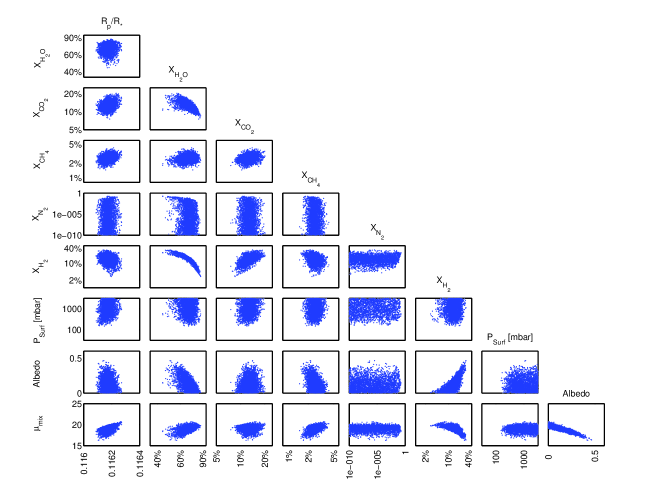
An inherent correlation arises between the planetary albedo and the mean molecular mass (Figure 11) if no direct measurements of the planetary temperature or the planetary albedo are available. While the correlation does not lead to uncertainties of individual parameters that range over orders of magnitude, it can be the dominant source of uncertainty on the composition if small error bars are achieved for the observations of the primary transit, but no direct measurements of the brightness temperature or the planetary albedo are available from secondary eclipse observations .

The reason for the correlations between mean molecular mass and albedo is that the primary observables for the mean molecular mass (see Section 4.1.2) constrain the scale height rather than the mean molecular mass directly. Given the observational constraints for the scale height, different combinations of the atmospheric temperature and mean molecule mass may agree equally well with the scale height constraints imposed by the spectrum. The atmospheric temperature, in turn, is primarily determined by the planetary albedo, giving rise to the correlation between planetary albedo and mean molecular mass.

A higher mixing ratio of $\mbox{H}_{2}$ lowers the mean molecular mass without creating new absorption features. An atmosphere with more $\mbox{H}_{2}$ and less of the main constituent (here: $\mbox{H}_{2}\mbox{O}$) in conjunction with an increased planetary albedo shows virtually the same transmission spectrum as the one shown in Figure 8. As a result, the posterior distribution shows a significant correlation between $X_{\mathrm{H_{2}}}$ and the Bond albedo as well as between $X_{\mathrm{H_{2}}}$ and $X_{\mathrm{H_{2}O}}$ (Figure 11).

?figurename? 11.— Two-dimensional marginalized probabilities for pairs of atmospheric properties for simulated JWST NIRSpec observations of the "Hot Halley world" scenario for GJ 1214b. The synthetic observation used for the atmospheric retrieval is illustrated in Figure 8. For observations that cover all $n+4$ observables discussed in Section 4.1, the posterior distribution of the atmospheric parameters retrieval lacks degeneracies or strong correlations that would keep individual parameters unconstrained over orders of magnitude (Figure 11). Planetary albedo and the mean molecular mass show a correlation because different combinations of atmospheric temperature and mean molecular mass may lead to the same scale height and, therefore, to similar spectral feature shapes.

4.3. Elemental Abundances

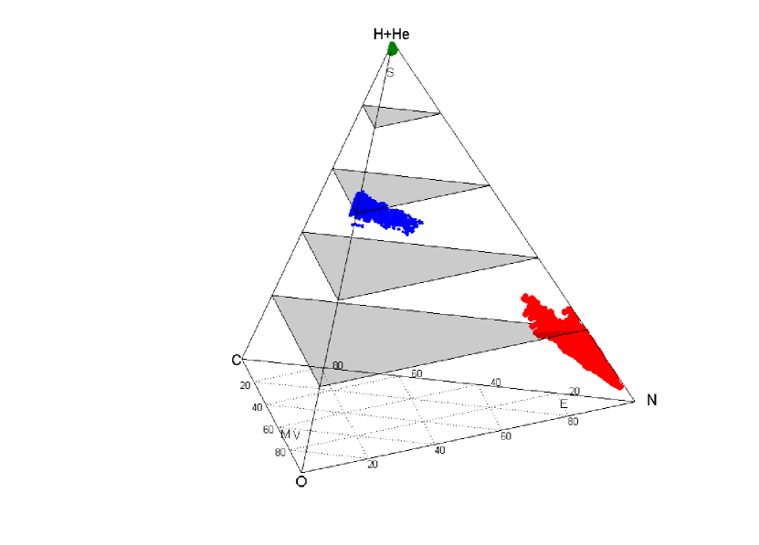
The ability to constrain the mixing ratios of both the absorbing and the spectrally inactive gases in the atmosphere provides us with the opportunity to probe the relative abundances of the volatile elements H, C, O, and N of the atmospheres of exoplanets. Conceptually, the retrieval of the elemental abundances in the atmosphere is directly linked to the retrieval of the molecular mixing ratios, since the constraints on elemental abundances are derived from the probability density distribution of the molecular mixing ratios (Section 2.5). Following the result in the previous subsections, low-noise observations of moderate to high spectral resolution lead to well-constrained molecular mixing ratios and therefore also allow determination of well-constrained elemental abundances.

For quantitative constraints, we return to our three scenarios for hot super-Earth atmospheres. The transmission spectra can clearly discriminate the different relative abundances of the volatile elements in the three scenarios (Figure 12) and may be used to probe their formation history and evolution. The hot mini-Neptune scenario can be identified to have accreted and retained a primordial atmosphere dominated by hydrogen, similar to gas and ice giants in our solar system. At the other end of the parameter space, the elemental composition of the second scenario indicates an atmospheric composition dominated by nitrogen. The third scenario shows an atmosphere that has retained some hydrogen in heavier molecular species.

?figurename? 12.— Quaternary diagram illustrating the posterior probability distributions for the relative abundances of the elements H, C, O, and N. The colored volumes represent the 2$\sigma$ Bayesian credible regions of the elemental composition for the "hot Halley world" (blue), the "hot nitrogen-rich world" (red) and the "hot mini-Neptune" (green). The symbols E, M, V, and S indicate the elemental abundances in the atmospheres of the Solar System planets Earth, Mars, Venus and Saturn, respectively, for comparison. The four vertices of the diagram represent an atmosphere that is fully composed of H, C, O, or N. The opposing faces are surfaces on which the fraction of H, C, O, or N is zero. At each point inside the tetrahedron, the elemental fraction is given by the distances perpendicular to the faces.

4.4. Total Atmospheric Mass

We find that transmission spectra present an opportunity to determine a lower limit for the total mass of the atmosphere of extrasolar planets based purely on observations. Conceptually, the constraints on the total atmospheric mass are derived from the constraints on the composition and the surface pressure of the atmosphere. The ability to constrain mixing ratios of both the absorbing and the spectrally inactive gases in the atmosphere enables us to constrain the mean molecular mass and therefore the mass density in the atmosphere as a function of pressure. Combined with the independent constraints on the surface pressure, we can integrate the mass density to estimate the total column density of the atmosphere. Under the assumption of an approximately uniform bulk composition and surface pressure around the spherical planet, we therefore obtain a constraint on the total mass of the atmosphere.

Two fundamental limits prevent one from accurately constraining the total atmospheric mass. First, the mass determined from transmission spectra corresponds to the total atmospheric mass above the uppermost surface (see Figure 10(f) for a quantitative example). Second, following the arguments on the retrieval of the surface pressure (Section 4.1.4), we will not be able to detect the uppermost surface explicitly if the cloud-free part of the atmosphere is sufficiently thick (Figures 8 and 9). In conclusion, we can always determine a lower limit on the atmospheric mass once we have detected spectral features, but determining an upper limit is only possible if the atmosphere is sufficiently thin for the surface to be detected and an opaque cloud deck can be excluded from theoretical principles.

5. Discussion

5.1. Obtaining Observational Constraints on Atmospheric Composition

The objective in the development of the new retrieval methodology was to remain independent of model assumptions as much as possible and let the observational data speak for themselves. By not employing any assumptions on the elemental composition, chemical equilibrium, or formation and evolution arguments in the retrieval process, our results remain independent of preconceived ideas for the planet under investigation. The atmospheric composition is, instead, completely described by free parameters and no hidden biases or asymmetries favoring a particular molecular species in the Bayesian prior are introduced.

The main assumptions in our approach are limited to the principles of radiative transfer in local thermodynamic equilibrium, hydrostatic equilibrium, and the correctness of the molecular line lists. For cases in which no secondary eclipse measurements are available, we added radiative-convective equilibrium to determine a reasonable temperature structure. However, since the exact temperature profile has a secondary effect on the transmission spectrum, we find that this temperature modeling has little effect on the retrieval results we obtain. In order to reasonably constrain the atmosphere given the limited data available in the near future, another guideline in the development was to keep the number of parameters to a minimum, while still ensuring that the parameters uniquely define the state of the model atmosphere. In this study, we assigned a single free parameter for the effective mixing ratio of each molecular species in the atmosphere, effectively comparing well-mixed atmospheres to the observation (see Section 5.3).

The main advantage of our retrieval approach for super-Earths over detailed modeling of atmospheric chemistry and dynamic models is that it provides an opportunity to discover unexpected types of planets and atmospheres that do not agree with our current understanding of formation, evolution and atmospheric processes. For example, no self-consistent atmospheric chemistry model would predict that the atmosphere of a terrestrial planet like Earth has an $\mathrm{O_{2}}$ mixing ratio as high as 21%. Only the direct interpretation of observations can tell us about the existence of such unusual atmospheric compositions. The identification of absorption lines of the $\mathrm{O_{2}}$ absorption without constraining the high mixing ratio would not be a biosignature because low abundances of $\mathrm{O_{2}}$ can be a result of photochemical composition.

In this work, we have shown that we can quantitatively constrain the atmospheric composition based on observations of the transmission spectrum, even for super-Earth planets for which the composition is completely unknown a priori. Transmission spectroscopy is a good tool for retrieval of the composition because the absorber amount and mean molecular mass are the main drivers determining the features of the transmission spectrum, while the influence of the unknown temperature profile is secondary. We also find, however, that the characterization of super-Earth planets requires considerably more spectral coverage and precision than the characterization of the hydrogen-dominated atmospheres of hot Jupiters. This is not only because of the smaller signal, but also because of a more complex parameter space that can result in degeneracies.

5.2. Non-Unique Constraints for Hazy Atmospheres

Photochemically-produced hazes may have a significant opacity at short wavelengths and may mask the signature of molecular Rayleigh scattering if they are present in the upper atmosphere, . While we may still be able to probe the near-infrared spectrum and identify molecular absorbers, we will not be able to probe the transit depth offset of Rayleigh scattering due to molecular scattering. Without making further assumptions, we will, therefore, lose the ability to constrain the mixing ratio of the molecular species over orders of magnitude, even for the major constituents of the atmosphere (see Section 4.1).

By measuring either the slope of the Rayleigh scattering signature or the shapes of molecular absorption features, we will still obtain information on the scale height of the atmosphere and, therefore, obtain an estimate on the mean molecular mass (Section 4.1.2). We will not, however, be able to constrain the total amount of the spectrally inactive gases. Since the near-infrared spectrum only constrains the relative abundances of the absorbing gases (Section 4.1.1), we can hypothesize different atmospheric mixtures of $\mbox{H}_{2}$, $\mbox{N}_{2}$, and absorbing gases in the correct ratiosthat produce nearly identical transmission spectra. As a result, we obtain a degeneracy that prevents us from constraining the molecular abundances uniquely.

One assumption that could be made to compensate for the lack of information is to not consider the simultaneous presence of nitrogen gas, $\mbox{N}_{2}$, and hydrogen gas, $\mbox{H}_{2}$. In general, however, the simultaneous presence of $\mbox{N}_{2}$ and $\mbox{H}_{2}$ cannot be excluded, even though the preferred chemical form of the two elements N and H in chemical equilibrium is ammonia $\mbox{NH}_{3}$ at a wide range of temperatures and pressures because the energy barrier for the reaction is too large due to strong triple bonds in nitrogen molecules.

5.3. Stratified Atmospheres

Our parameterization of the atmosphere in the retrieval process assumes a well-mixed atmosphere. Given the limited amount of data available in the near-future, the motivation for the assumption of well-mixed atmospheres is to keep the number of free parameters, which make use of similar information in the spectrum, small. Observations of the Solar System planets justify the approach because $\gtrsim$95% of the gas in each of the Solar System atmospheres is composed of long-lived, chemically stable species that were mixed by turbulence and diffusion for a sufficiently long time (see Lodders & Jr, 1998; Pater & Lissauer, 2010, and reference therein). If exquisite observations become available in the future, however, it may be useful to extend the parameterization to retrieve compositional gradients. For some molecular species, such gradients may be identified as biomarkers caused by sources at or in the planetary surface.

Physical effects that lead to compositional stratifications of the gaseous species in the Solar System atmospheres are (1) condensation of gases that condense at pressure and temperature levels encountered in the atmosphere, or (2) production or destruction of gas by photochemistry or geology, or (3) variation of chemical equilibrium with altitude due to the altitude dependencies of pressure and temperature. Changes of gas concentration with altitude that are caused by condensation, however, are usually not relevant for our retrieval because transmission spectroscopy only probes layers above the condensation clouds. Similarly, strong changes in the chemical equilibrium usually occur at deep levels in thick envelopes that are unlikely to be probed in transmission. In addition, the mixing ratios of gases that do vary with altitude often only vary over less than one order of magnitude, e.g., CO, $\mbox{H}_{2}\mbox{O}$, $\mbox{SO}_{2}$ in the atmosphere of Venus (Hunten, 1983). Observational data that are less noisy than the synthetic JWST observations considered in Section 4.2 are necessary to robustly detect such gradients because the retrieved mixing ratios for minor species in the synthetic JWST observations are uncertain to within one order of magnitude, even for well-mixed atmospheres (Section 4.2). Photochemistry or surface sources, however, may lead to concentration gradients that are substantial at pressure levels probed by transmission spectroscopy (e.g., ozone in Earth’s atmosphere) and may justify extensions to our parameterization in the future.

For atmospheres with a stratified composition, our retrieval method determines an altitude-averaged mixing ratio that best matches the observed transmission spectrum. In test cases, we verified that the atmospheric retrieval method remains robust in providing a reasonable estimate for the mixing ratios for stratified atmospheres. We simulated transmission spectra for stratified atmospheres and performed the retrieval assuming a well-mixed atmosphere (Figure 13). We found that, the method remains robust and the retrieved mixing ratios for stratified gases correspond to the mixing ratios at the pressure levels at which the functional derivatives with respect to the mixing ratio are the highest. Using the functional derivatives, we can, therefore, estimate a posterior at which pressure level we have probed the atmospheric mixing ratio of the gas.

?figurename? 13.— Atmospheric retrieval for stratified atmospheres. The left panel illustrates the volume mixing ratio profiles used to simulate the synthetic JWST observations for a stratified atmosphere scenario. In this scenario, the volume mixing ratio $X_{\mathrm{CO_{2}}}$ is chosen to decrease log-linearly from 5% at 1 bar down to 0.1% at 0.01 mbar. The error bars of the observations are similar to ones in Figure 9 (synthetic observations are not shown). The middel panel illustrates the marginalized posterior probability density as obtained when performing atmospheric retrieval on the synthetic observations. The abundances of all molecular species are robustly retrieved. The most likely value for $X_{\mathrm{CO_{2}}}$ matches the value at the 1-10 mbar level because the functional derivatives—averaged across the observed spectrum—are highest for this pressure level (right panel).

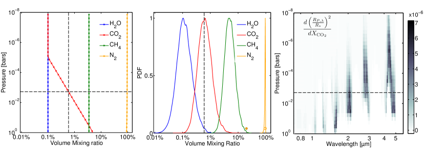
5.4. A Predictive Tool for Planning Observational Programs and Designing Future Telescopes

Additional applications of the retrieval method presented here are (1) to evaluate and optimize observational strategies in the planning and proposal process of exoplanet observations and (2) to guide the design of future telescopes and instrumentation for the characterization of exoplanets. Numerical studies using the retrieval method can provide concrete guidelines on how many transits must be observed and what spectral range and spectral resolution is ideal for a specific atmospheric characterization. The motivation behind the approach is that observational characterizations of super-Earth atmospheres are extremely challenging and the observation of many transits with highly capable observatories will be required.

While the retrieval method is not essential to recognize the need for higher S/N data than currently available, the retrieval method is critical to determining exactly what magnitude of data is required for a useful atmospheric characterization. GJ 1214b is a good example: In the past, 1 or 2 transits were observed at different wavelengths by various observers with the goal to characterize the atmosphere (Bean et al., 2010, 2011; Croll et al., 2011; Berta et al., 2012). Even though some of these observations approached the theoretical photon limit, few constraints on the atmosphere could be found. Retrieval analysis on simulated data shows that ten or more transits are required with currently available observatories in order to separate out the two currently most plausible scenarios of a water world and a hydrogen-dominated atmosphere with high-altitude clouds (B. Benneke et al., in preparation). We propose a new paradigm in planning observations in which retrieval analysis of synthetic observations can quantitatively justify the necessity of large campaigns with ground-based or space-based observatories for atmospheric characterization.

A conceptually understanding of which details in the spectrum are required to constrain the atmospheric composition will enable observers to rationally select the wavelength ranges and spectral resolutions of transit observations for atmospheric characterization. For example, constraining the volume mixing ratios of molecular absorbers in super-Earth atmospheres will require measuring the Rayleigh scattering signature in addition to the molecule’s absorption signatures in the infrared. If the Rayleigh scattering signature is not observed, even low-noise observations of the spectral features in the near-infrared with JWST will not provide the information required to determine the volume mixing ratios.

In addition to the general results, we used simulated JWST NIRSpec observations covering the full range from $\mathrm{0.6}$ to $5\,\text{$\mu$m}$ to show which quantitative constraints on the composition could be obtained with JWST NIRSpec. An assessment of how well the different atmospheric properties can be constrained, how many transits are needed, or what observational parameters are optimal needs to be done with a specific scientific objective and the available instruments in mind. Therefore, we envision to use the methodology in the future in collaboration with observers to evaluate near-future observational opportunities with currently available instruments.

5.5. Compositional Retrieval versus Detailed Atmospheric Modeling

The atmospheric retrieval method and detailed, self-consistent modeling of a planetary atmosphere (Burrows et al., 1997; Seager et al., 2005; Burrows et al., 2008) present two completely complementary approaches to the study of planetary atmospheres. For studies of solar system planets, it is common practice to use observational constraints from remote sensing to motivate or validate detailed modeling of chemistry or dynamics. For a classic example, the retrieved temperature-pressure profile from radio occultation measurements on Titan motivated and guided detailed modeling of the thermal structure to explain the measured temperature profile (McKay et al., 1989). Similarly, the observational detection and abundance constraints on the methane plume in the Martian atmosphere motivated a multitude of studies on potential sources and sinks (e.g., Lefevre & Forget, 2009; Krasnopolsky et al., 2004).

We envision the same kind of complementarity for the characterization of exoplanets. The strategy would be to use the retrieval method as presented in this work to identify quantitative constraints on the atmospheric composition provided by the observations. Then, the constraints on elemental or molecular abundances can serve as inputs to help guide the detailed atmospheric modeling to explore physical processes that would explain the findings. Conversely, atmospheric retrieval can be complemented by self-consistent forward models in that self-consistent modeling can further constrain the parameter space by checking the physical plausibility of the atmospheric scenarios.

Chemistry-Transport and Photochemistry Models

While self-consistent forward models of atmospheric chemistry aim to provide the physical understanding of the relevant processes in the atmosphere, self-consistent forward models are dependent on inputs such as the background atmosphere or elemental abundances, the boundary conditions at the surfaces, as well as an accurate representation of all relevant chemical reactions, heat transport and cloud formation processes. If we knew all inputs and relevant processes a priori, one could compute the chemical composition and state of the atmosphere with a self-consistent model. However, many of these inputs will not be known for exoplanets, especially for planets that do not agree with our preconceived ideas.

Atmospheric retrieval provides an alternative to self-consistent modeling forobtaining the composition and state of the atmosphere, but is based on observations rather than detailed modeling. It can, therefore, guide the development and application of self-consistent models in providing constraints on the background atmosphere as well as constraints on the minor species in atmosphere. As the background atmospheres of super-Earth planets are not known a priori, it appears that most self-consistent models of atmospheric chemistry will require that one uses atmospheric retrieval to infer at least the main species in the atmospheres of these objects. If the self-consistently modeled atmospheric properties deviate from the ones provided by the retrieval analysis of given a set of observations, then the analysis of the deviation may motivate the inclusion of additional physical or chemical processes to the self-consistent model (e.g., additional sources and sinks for molecular species). The combination of self-consistent modeling and atmospheric retrieval to interpret observations can, therefore, enhance our understanding of the physical processes in the atmospheres of extrasolar planets.

Atmospheric Dynamics

One of the most critical factors affecting atmospheric circulation models is determining the pressure level at which the bulk of the stellar energy is deposited (Heng, 2012; Perna et al., 2012). Atmospheric retrieval may provide a useful input to determine this pressure level for an observed exoplanet because it allows the constraint of the molecular composition of the atmosphere, which strongly affects the opacity of the atmosphere to the incident stellar flux. For hot Jupiters, previous studies (e.g., Showman et al., 2009) assumed chemical equilibrium in combination with solar composition as a fiducial estimate of the composition. When modeling a specific planet, the danger is that these assumptions for the composition introduce inaccuracies in the deposition of stellar light and therefore alter the results.

For circulation modeling of super-Earth atmospheres, obtaining observational constraints on the atmospheric properties is critical. Without observations or a better understanding of super-Earth planets, even the main constituents of these atmospheres are unknown, and therefore no fiducial assumptions on the composition and stellar flux deposition can be made. For rocky planets, the presence of a solid surface and the pressure level at the surface play a major role in the atmospheric circulation. The retrieved surface pressure from observations may, therefore, also provide an essential input for circulation models.

6. Summary and Conclusions

We have presented a Bayesian method to retrieve the atmospheric composition and thickness of a super-Earth exoplanet from observations of its transmission spectrum. Our approach is different from previous work on super-Earths in that we do not test preconceived scenarios, but retrieve constraints on the atmospheric properties governed by observations, assuming no prior knowledge of the nature of the planet. Our work extends previous work on atmospheric retrieval for hot Jupiters in that we introduce a parameterization that is applicable to general atmospheres in which hydrogen may not be the dominating gas and clouds may be present. We infer constraints on individual parameters directly by marginalizing the joint posterior probability distribution of the atmospheric parameters. The uncertainty of individual parameters introduced by complicated, non-Gaussian correlations with other parameters is, therefore, accounted for in an elegant and straightforward way.

In this work, we have applied the retrieval method to synthetic observations of the super-Earth GJ 1214b. We investigated which constraints on the atmospheres of super-Earth exoplanets can be inferred from future observations of their transmission spectra. Our most significant findings are summarized as follows.

• A unique constraint of the mixing ratios of the absorbing gases and up to two spectrally inactive gases is possible with moderate-resolution ($R\sim 100)$ transmission spectra, if the spectral coverage and S/N of the observations are sufficient to quantify (1) the transit depths in, at least, one absorption feature for each absorbing gas at visible or near-infrared wavelengths and (2) the slope and strength of the molecular Rayleigh scattering signature at short wavelengths. Assuming that the atmosphere is wellmixed, and that $\mathrm{N_{2}}$ and a primordial mix of $\mathrm{H_{2}+He}$ are the only significant spectrally inactive components, one can therefore uniquely constrain the composition of the atmosphere based on transit observations alone.

• We can discriminate between a thick, cloud-free atmosphere and an atmosphere with a surface, where the surface is either the ground or an opaque cloud deck. For an atmosphere with a surface at low optical depth, we can quantitatively constrain the pressure at this surface. A unique constraint of the composition is also possible for an atmosphere with a surface.

• An estimate of the mean molecular mass made independently of the other unknown atmospheric parameters is possible by measuring either the slope of the Rayleigh scattering signature, the shape of individual absorption features, or the relative transit depths in different features of the same molecular absorber. For super Earths, discriminating between hydrogen-rich atmospheres and high mean molecular mass atmospheres is, therefore, possible, even in the presence of clouds.

• Determining the volume mixing ratios of the absorbing gases relies on observations of the molecular Rayleigh scattering signature. Although the presence of most molecular species can be identified in the near-infrared, only the relative abundances of the absorbing molecules can be determined from the infrared spectrum, not their volume mixing ratios in the atmosphere. The Rayleigh signature of molecular scattering is required because it enables the measurement of the abundances of spectrally inactive gases. If the molecular Rayleigh scattering cannot be observed or is masked by haze scattering at short wavelengths, we will not be able to determine the volume mixing ratio of the gases in the atmosphere to within orders of magnitude. The drastic inability to constrain the mixing ratio was not discovered in previous work on atmospheric retrieval because hot Jupiters were assumed to be cloud-free and the mean molecular mass in a hydrogen-dominated atmosphere was known a priori (e.g., Madhusudhan & Seager, 2009).

• The retrieval of the mixing ratios of spectrally inactive gases is fundamentally limited to two independent components. An inherent degeneracy arises if the atmosphere contains three or more independent spectrally inactive gases because the same mean molecular mass and the same strength of the Rayleigh scattering signature can be obtained with different combinations of the gases.

• Non-Gaussian treatments of the uncertainties of atmospheric parameters are essential for atmospheric retrieval from noisy exoplanet observations. Even given low-noise synthetic observations as considered in this work, only one-sided bounds and highly non-Gaussian correlations exist for some atmospheric parameters. Non-Gaussian effects will become stronger for observational data sets noisier than the synthetic data considered in this work because the relation between the observables and the desired atmospheric parameters is highly nonlinear and larger volumes of the parameter space become compatible with noisier observations. A limitation of optimum estimation retrieval (Lee et al., 2011; Line et al., 2012) for the analysis of noisy exoplanet spectra is, therefore, that the extent of the confidence regions of atmospheric properties cannot correctly be described by Gaussian errors around a single best-fitting solution.

Our findings indicate that the retrieval method presented here, combined with low-noise observations, will provide the opportunity to observationally characterize atmospheres of individual super-Earth planets and uniquely identify their molecular and elemental compositions. Similar to observational constraints on the atmospheres of the Solar System planets obtained over the last decades, the quantitative constraints obtainable with our atmospheric retrieval will generally be independent of preconceived ideas of atmospheric physics and chemistry as well as planet formation scenarios and atmospheric evolution. The unbiased constraints can, therefore, motivate the detailed study of the new phenomena in atmospheric dynamics and chemistry, identify habitability and biosignatures, or provide clues to planet formation and atmospheric evolution.

We thank Leslie Rogers, David Kipping, Renyu Hu, Julien de Wit, and Brice Demory for very helpful discussions. We thank Larry Rothman for access to the HITRAN and HITEMP databases. Support for this work was provided by NASA.

?appendixname? A An Algebraic Solution to Infer the Mean Molecular Mass

For thin or cloudy atmospheres the change in the transit depth across the spectrum, $\Delta D$, as proposed by Miller-Ricci et al. (2009), cannot be used to uniquely constrain the mean molecular mass because clouds, hazes, and a surface also affect the feature depths. Here, we show that measuring the linear slope of the Rayleigh scattering signature or the shapes of individual features, instead, does provide constraints on the atmosphere scale height and can be used to estimate the mean molecular mass for general atmospheres independently of other atmospheric properties. We derive an algebraic solutions that can be used to infer the mean molecular mass directly from the transmission spectrum.

From the geometry described by Brown (2001), we obtain the slant optical depth, $\tau(b)$, as a function of the impact parameter, $b$, by integrating the opacity through the planet’s atmosphere along the observer’s line of sight:

$$\tau_{\lambda}\left(b\right)=2\intop_{b}^{\infty}\sigma_{\lambda}\left(r\right)n\left(r\right)\frac{r\,dr}{\sqrt{r^{2}-b^{2}}}.$$ (A1)

Here, $r$ is the radial distance from the center of the planet. For Rayleigh scattering, the extinction cross section is only very weakly dependent on pressure and temperature, and we can assume $\sigma_{\lambda}\left(r\right)=\sigma_{\lambda}$. Furthermore, motivated by hydrostatic equilibrium, we assume that the atmospheric number density falls off exponentially according to $n\left(r\right)=n_{0}e^{-\frac{r}{H}}$, where $H$ is the atmospheric scale height. With these assumptions we can analytically perform the integration in Equation (A1) and obtain

$$\tau_{\lambda}\left(b\right)=2n_{0}\sigma b\mathcal{K}_{1}\left(\frac{b}{H}\right)\approx 2n_{0}\sigma b\sqrt{\frac{\pi}{2\frac{b}{H}}}e^{-\frac{b}{H}},$$ (A2)

where the modified Bessel function of the second kind $\mathcal{K}_{1}\left(x\right)$ is approximated by its asymptotic form $\mathcal{K}_{1}\left(x\right)=\sqrt{\frac{\pi}{2x}}e^{-x}\left[1+O\left(\frac{1}{x}\right)\right]$ for large $x$ (Bronstein et al., 1999). For spectral regions, for which the atmosphere is optically thick, the surface does not affect the transmission spectrum and the observed planet radius as a function of wavelength can be approximated as

$$R_{P,\lambda}\approx b\left(\tau_{\lambda}=1\right),$$ (A3)

because the number density falls exponentially with altitude leading to steep increase in $\tau_{\lambda}$ as a function of $b$. Forming the ratio between the radii at two different wavelengths, $\lambda_{1}$ and $\lambda_{2}$, for which the extinction cross sections are $\sigma_{1}$ and $\sigma_{2}$, and solving for the scale height, we obtain

$$H|_{r=R_{P}}\approx\frac{R_{P,2}-R_{P,1}}{\ln\left(\frac{\sigma_{2}}{\sigma_{1}}\sqrt{\frac{R_{P,2}}{R_{P,1}}}\right)}\longrightarrow\frac{dR_{P,\lambda}}{d\text{ $\ln\left(\sigma_{\lambda}\sqrt{R_{P,\lambda}}\right)$}}\approx\frac{dR_{P,\lambda}}{d\text{$\left(\ln\sigma_{\lambda}\right)$}},$$ (A4)

where we considered the limit of $\lambda_{1}\rightarrow\lambda_{2}$ and then approximated for $\frac{d\ln R_{p,\lambda}}{d\ln\sigma_{\lambda}}$$\ll 1$.

Given an estimate of the atmospheric temperature, e.g., $T\approx T_{\mathrm{eq}}$, we can observationally determine an estimate on the mean molecular mass

$$\mu_{\mathrm{mix}}=\frac{k_{B}T}{g}\left(\frac{dR_{P,\lambda}}{d\text{$\left(\ln\sigma_{\lambda}\right)$}}\right)^{-1}\times\left(1\pm\frac{\delta T}{T}\right),$$ (A5)

where the factor $\left(1\pm\frac{\delta T}{T}\right)$ accounts for the inherent uncertainty due to the uncertainty, $\delta T$, in modeling the atmospheric temperature, $T$, at the planetary radius $r=R_{P,\lambda}$.

At short wavelengths for which Rayleigh scattering dominates, the extinction cross section $\sigma$ is proportional to $\lambda^{-4}$, and we obtain

$$H\approx\frac{R_{P,\lambda_{2}}-R_{P,\lambda_{1}}}{4\ln\left(\frac{\lambda_{1}}{\lambda_{2}}\right)}.$$ (A6)

Given two transit depth observations at $\lambda_{1}$and $\lambda_{2}$ in the Rayleigh scattering regime, we obtain the estimate for the mean molecular mass

$$\mu_{\mathrm{mix}}=\frac{4k_{B}T}{gR_{*}}\frac{\ln\left(\frac{\lambda_{1}}{\lambda_{2}}\right)}{\left(\frac{R_{p}}{R_{*}}\right)_{\lambda_{2}}-\left(\frac{R_{p}}{R_{*}}\right)_{\lambda_{1}}}\times\left(1\pm\frac{\delta T}{T}\right).$$ (A7)