Scilab and SIP for Image Processing

Abstract

This paper is an overview of Image Processing and Analysis using Scilab, a free prototyping environment for numerical calculations similar to Matlab. We demonstrate the capabilities of SIP – the Scilab Image Processing Toolbox – which extends Scilab with many functions to read and write images in over 100 major file formats, including PNG, JPEG, BMP, and TIFF. It also provides routines for image filtering, edge detection, blurring, segmentation, shape analysis, and image recognition. Basic directions to install Scilab and SIP are given, and also a mini-tutorial on Scilab. Three practical examples of image analysis are presented, in increasing degrees of complexity, showing how advanced image analysis techniques seem uncomplicated in this environment.

1 Introduction

Image Processing and Analysis are fields of Computer Science whose objective is to enhance digital images and extract information from them [1, 2, 3]. This allows automatic or semi-automatic identification, classification or characterization of objects and patterns. Some interesting applications are biometry systems (e.g. fingerprint and iris recognition), satellite and microscope image analysis, diagnosis from medical images, and more. Another example is special effect filtering, usually found in image manipulation software such as the gimp [4] or Photoshop.

A remarkable characteristic of this field is its overwhelming complexity. Many image processing techniques are based on sophisticated mathematical and computational concepts, such as the Fourier Transform. All this is combined with deep biological, psychological and probabilistic principles underlying the way animals identify and recognize objects. This makes implementation a challenging (frequently tedious) task , specially with traditional languages such as C or Fortran. As a consequence, the area had been somewhat limited to a small community of scientists and programming experts.

The difficulties involving the development of software in general and the advances in hardware power gave rise to a quite recent trend in programing [5] – prototyping with interpreted, easy-to-use languages, such as Python, Perl, Lua, and Tcl/Tk. Different algorithms and solutions for a given problem are easily developed and validated using these environments. When a solution finally works as expected, the final application may be written in a traditional compiled language, such as C. Many programmers also embed an interpreter in their final application, to reuse the large amount of functionality available in these environments without having to rewrite it all.

Following this trend, the inherent complexity of scientific applications called for specific scripting technologies. Among them is the popular (and rather expensive) Matlab [6], very widely used in science, engineering, and the industry. Fortunately there are free software alternatives such as Octave [7], numerical Python [8], and Scilab [9] – the one we will be talking about in this paper. Features common to all these numerical prototyping environments are convenient matrix manipulation enforced by a suitable language, as well as tools for scientific visualization, debugging, and a great ammount of easy-to-use libraries. They may be used interactively or programmed from a separate file (the ‘script’ or ’macro’). In particular, they enable development of Image Processing applications with much less burden to the programmer. Hence, these tools have in fact been the standard prototyping solutions in the field.

Scilab is a free software created at INRIA–France for prototyping and numerical processing. It is much like Matlab, and already has a rich set of functionalities. Currently in version 5.4, Scilab have been widely used in Unix-like systems. It has been adopted in many Universities and companies around the world. Given its features to assist numerical programming, as we just said, it has tremendous potential to be used for image processing, both educationally and as a prototyping language to develop and test solutions. As far as we know, currently neither Octave or Python match the richness and plain simplicity of scilab functionality for scientific computing and engineering.

The following listing summarizes Scilab’s features and how they compare to Matlab’s:

• Expressive programming language with similar syntax to Matlab’s, although not identical. It presents many sophisticated construct improvements over Matlab, having relatively small drawbacks. Moreover, operations are expressed in much the same way they are usually written mathematically, which enforces simplicity and organization.

• Elaborate data structures: polynomial, complex and string matrices, lists, linear systems, records (tlists), and graphs. In these subjects there are significant improvements over Matlab.

• Graphical and Scientific Visualization library: 2D, 3D, and animations. Even though the graphical package is not as stable as Matlab, it is useful and complete. It has been continually improved and optimized. The GUI itself has now been written in Java, and looks and feels very similar – if not better – than Matlab.

• Modular structure: Scilab allows easy interfacing to Fortran and C using dynamic linking.

• Many sophisticated libraries:

  • Linear Algebra, including sparse matrices.

  • Signal Processing with a comprehensive manual;

  • Statistics

  • Scicos, a dynamic systems modeler and simulator, similar to Matlab’s Simulink.

  • Metanet: graphs and networks, including a graphical editor

  • Control

  • Simulation and Modeling: ODE solver, etc.

  • Optimization (differential and non-differential)

  • Interface with symbolic algebra packages such as Maple

  • Interface with Tcl/Tk, useful for building GUI’s

  • LMI optimization (Linear Matrix Inequalities)

  • Many contributed libraries: genetic algorithms, neural networks, plotting enhancements, other numerical methods, and, of course, image processing.

Scilab’s potential for imaging and its maturity under GNU/Linux systems motivated the creation of SIP – the Scilab Image Processing Toolbox [10]. SIP extends Scilab with many routines to deal with image files and analyze them. Examples of its main features are:

• Functions to read and write many image formats. Almost 100 major formats are supported, including JPEG, PNG, BMP, GIF, and TIFF – due to the underlying ImageMagick library [11].

• Filters: Gaussian blurring, median, Laplacian, artistic effects, de-noising by min-max curvature flow.

• Edge detection: Sobel, Fourier derivatives, Canny.

• Geometric transforms: rotation, zoom, shearing, and general affine.

• Image segmentation: watersheds, adaptive thresholding.

• Mathematical morphology: dilation, erosion, thinning, etc., using state-of-the-art Euclidean algorithms for circular structuring elements.

• Shape analysis: perimeter, border tracking, state-of-the-art fast skeletonization with multiscale pruning, curvature, state-of-the-art Euclidean distance transforms [12] (including fast distance transforms up to a given distance), fractal dimension.

• Enhancement: histogram equalization, contrast manipulation.

• Other operators: Hough transform, noise generation, image display, interferometry operations (e.g. phase unwrapping), etc.

• It’s fast: heavier operations are implemented in C language, allowing for efficiency. Many operations use state-of-the-art efficient algorithms, some of which are so new or advanced as to be absent in most if not all proprietary image analysis software.

• It’s well documented: Every function has a help page containing its reference and a practical example.

• It’s free: General Public License (GPL).

• It’s easy: Useful for fast programming and experimentation.

All these tools can be easily used interactively or from scilab scripts, even though some would extremely complex to implement from scratch. Thus, a programmer without specialized knowledge may readily experiment with different techniques to solve his particular problem.

In this paper we show how to use SIP/Scilab and demonstrate their benefits through a hands-on approach. The examples will show how complex operations seem approachable under the expressiveness of the environment. Rather than worrying about a single imaging operator, the focus is shifted to the concatenation of various operators into a useful solution.

We start with brief directions on how to install Scilab under Linux and present a tutorial introduction to it. We then show how to install SIP and use it in three practical problems from Image Analysis and Processing: edge detection, OCR, and separation of overlapping blood cells. The last two illustrate techniques like noise removal, skeletonization, and object segmentation.

2 Customized Scilab Installation

To build a special version of Scilab by compiling the sourcecode, the user must have all development packages installed in the system (GCC and gfortran compilers, and so on). After downloading and unpacking the source tarball, one types the following inside Scilab’s directory:

      $  ./configure
      $  make all
      $  make install

To start scilab:

      $ scilab

One may enter commands in the scilab window, as shown in the following section. There is an important add-on toolbox called “Enrico” which greatly enhances Scilab’s graphical capabilities. It is very simple to install, and may be downloaded at: http://www.weizmann.ac.il/ fesegre/scistuff.html

The user must unpack it, start Scilab, then type:

--> exec ’/path/to/ENRICO/builder.sce’;

This compiles the toolbox. The user may now load it:

--> exec ’/path/to/ENRICO/loader.sce’;

This command may be placed in the “.scilab” file to load it automatically whenever one enters Scilab. In section 7 we show how to render a 3D surface using this toolbox (see figure 6).

3 A Mini Tutorial on Scilab

In this section we present some examples to illustrate the ease of doing programming and calculations with Scilab. We hope to attest its particularly great potential for programming and for developing image analysis solutions. Initially, we use Scilab in interactive mode. Commands are typed and executed directly in Scilab’s shell.

A vector is created like this:

--> a = [1 2 3 4]
 a  =

!   1.    2.    3.    4. !

User commands are typed at the ‘-->’ prompt; Scilab’s responses have no preceding prompts. To define a column vector, we use commas:

--> a = [1; 2; 3; 4]
 a  =

!   1. !
!   2. !
!   3. !
!   4. !

This same vector could have been created using the ‘:’ (colon) operator:

--> a = 1:4
 a  =

!   1.    2.    3.    4. !

Matrices are also very simple to define, as shown below:

--> a = [1 2; 3 4]
 a  =

!   1.    2. !
!   3.    4. !

Scilab have convenient operators for naturally manipulating matrices. For instance, to obtain the trasposed matrix of $a$:

--> b = a’
 b  =

!   1.    3. !
!   2.    4. !

In this other example, we perform matrix multiplication of $a$ and $b$:

--> c = a*b
 c  =

!   5.     11. !
!   11.    25. !

Scilab also has many functions readily available for usage. Below we calculate the determinant of $c$:

--> d = det(c)
 d  =

    4.

In addition to the simplicity of operating with arrays, there are many other mathematical functions, as well as visualization facilities. We will now show this by a simple example about the Fourier transform.

As the first step, we create a vector by summing three sampled cosines:

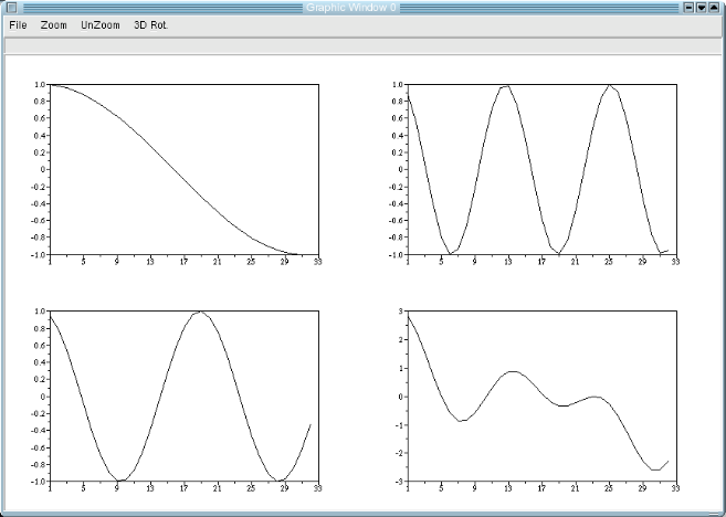
--> a  = 1:32;  // an array with 32 elements (1 to 32).
--> c1 = cos(a/10);
--> c2 = cos(a/2);
--> c3 = cos(a/6);
--> c  = c1 + c2 + c3;

Now we plot the vectors. We’ll use a simple function called plot for this, together with the command subplot to divide the graphical window. The commands below yield figure 1.

--> subplot(2,2,1), plot(c1);
--> subplot(2,2,2), plot(c2);
--> subplot(2,2,3), plot(c3);
--> subplot(2,2,4), plot(c);

Figure 1: Plots of vectors c1, c2, c3, and c

We will now apply the Fourier transform to the vector c, using function fft from the signal processing toolbox. Notice how simple it is:

--> hc = fft(c,-1);

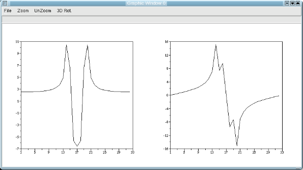
Observe that the second parameter indicates the sign of the transform’s exponent – it’s not the inverse transform. Vector hc is made of complex numbers representing the result of the fft applied to c. To see the results of the transform, lets use plot. Since a complex vector is composed of real and imaginary parts, we use the functions real and imag to return the real and imaginary components of the array. Figure 2 shows the plots of the real and imaginary parts of hc.

--> subplot(1,2,1), plot(real(fftshift(hc)));
--> subplot(1,2,2), plot(imag(fftshift(hc)));

Figure 2: Real (left) and imaginary part (right) of the complex vector hc

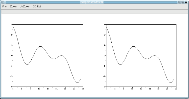
To finish this example, we perform the inverse FFT and compare the result with the original vector:

--> fc = fft(hc,1);
--> subplot(1,2,1), plot(fc);
--> subplot(1,2,2), plot(c);

Figure 3: Comparation between the inverse FFT and the original vector.

4 Installing the SIP Toolbox

The previous example shows how Scilab is really an easy and powerful for numerical programming and array manipulation. It would be great to use Scilab’s power and convenience to process digital images, since any image is an array of pixels. To do this, the SIP (Scilab Image Processing toolbox) was created (cf. section 1). It extends Scilab with functions to read and write images stored in almost any popular format (over 80), including PNG, JPEG, BMP, and TIFF. SIP also provides a rich set of ready-to-use operations for digital image enhancement and analysis, useful for many practical problems.

It is straightforward to install SIP under Linux. Binary packages are provided for Intel pentium and compatible processors. To install them, the user first downloads and unpacks the tarball. Inside Scilab, one types:

$  exec /path/to/sip/loader.sce;

This loads the toolbox. This command may be placed in the file .scilab under the user’s home directory to automatically load the toolbox whenever Scilab is entered.

For non-Intel architectures, SIP must be installed from source, which is also necessary to install the latest development version [13]. This requires first installing the dependencies, in this order: ImageMagick, Animal [14], OpenCV (optional), and finally SIP proper (cf. the links section). Once downloaded and unpacked, they are installed like this:

ImageMagick (responsible for the file format support):

      $  ./configure --enable-shared
      $  make
      $  make install
      $  ldconfig

The latter command updates the system cache of libraries.

Animal (core C routines):

      $  ./configure
      $  make
      $  make install
      $  ldconfig

SIP (the toolbox proper):

      $  ./configure
      $  make
      $  make install

SIP is by default installed under Scilab’s directory at ‘contrib/sip’. Now the toolbox may be loaded just like the binary version. Alternatively, one may type:

      $  make autoload

Which will write to the file .scilab and make the toolbox load automatically every time you enter Scilab. More details are found in the file INSTALL.txt included in the SIP sourcecode package. 

To check if the installation went well, the user steps through SIP’s demos:

$  exec(SIPDEMO);

Which shows the basics of image structure and manipulation.

5 Fundametal Image Operations

To read an image into a Scilab variable, one must type, for example:

--> im = imread(’myimage.png’);

for grayscale or truecolor images. Or

--> [im,map] = imread(’myimage.png’);

for pseudocolor images. The file format is automatically detected. From now on the image is in memory, stored as an array of pixels. We call grayscale those images represented as a 2D array with values from $0$ to $2^{16}-1$ $(65535)$. Truecolor images are made of three grayscale images, one for each channel (Red, Green and Blue), represented in a 3D array $(N\times M\times 3)$. Pseudocolor images, also known as paletted or indexed images, are made of two arrays: index and map. The map is an $(N\times 3)$ array with $N$ colors, while the index array is a 2D array whose entries point to a color in the colormap. Further details are in the introductory demo that comes with SIP.

To show a truecolor or grayscale image:

--> imshow(im);

For paletted images:

--> imshow(im,map);

To write an image:

--> imwrite(im,’foo.jpeg’);

or

--> imwrite(im, map,’foo.jpeg’);

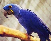
The next example is about edge detection, one of the most common operations in image processing [1]. First, let us read an image:

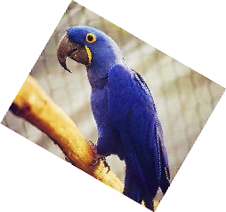
--> a = imread(’arara.jpg’);
--> imshow(a);
--> a = im2gray(a);       // converts to grayscale

The image is shown in figure 4.

Figure 4: Introductory example: (a) Read an image of an amazon bird, (b) extract edges from the image, and (c) rotate the image.

To find the edges, we use the ”edge” command:

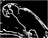
--> b = edge(a,’sobel’,0.15);
--> imshow(b,2);

The parameters means to find edges using the Sobel filter and a threshold at $15\%$ intensity level. Figure 4 shows the result of this technique.

Another common operation with images is rotation and scaling. The mogrify command wraps many functionalities from the ImageMagick library, and may be used to rotate the image. We must first put the image in the $0$ – $2^{16}-1$ range, because mogrify and other routines such as imwrite assumes 16bit graylevels. We just multiply the image by $257$, since $255*257=2^{16}$:

--> a = a*257;   // normalizes image to 0-65535 range
--> c = mogrify(a, ’-rotate 30’);   // rotates 30 degrees
--> imshow(c, []);  // "[]" stands for  rescaled

Figure 4 shows the color image rotated in 30 degrees clockwise. To rotate the color image, the same steps may be repeated to each image channel.

6 Example: OCR

Let us now move on to more interesting operations. Figure 5 shows an image of the letter A. To follow this example, the input image can be obtained from the following address:

http://siptoolbox.sourceforge.net/tutorial/images/a.png

Read the image with the following commands:

 a = imread(’a.png’);
 a = im2gray(a);    // converts to grayscale
 imshow(a);

Figure 5: Sample operations for shape recognition: (a) A noisy image; (b) gaussian blur; and (c) segmentation by threshold. Shape width is irrelevant for recognizing a letter, so we skeletonize the image (d), and simplify it using a technique called “multiscale pruning” (e).

Let us show a sequence of operations to help the computer recognize this letter. As the input, we have a noisy image, typically obtained from cheap CCD’s. We first Gaussian-blur [1] the image as to filter out the low-scale noise and leave our letter ‘A’ in clear evidence:

 b = gsm2d(a,2);  // Gaussian smoothing with sigma = 2
 imshow(b,[]);    // the [] parameter rescales b to 0-1

This is shown in figure 5. We may now perform thresholding with ease:

 c=im2bw(b,0.8); // threshold at the 80% level
 imshow(c,2);    // figure (c)

as shown in figure 5. This a much simpler representation for the letter A, with only two intensities. However, we can make it even simpler. The width of the letter is of no use to recognize it, so let us filter it out. We do this using a skeletonization algorithm, which finds a medial line of a given shape. In SIP, there is a novel fast implementation of a useul skeletonization algorithm [15, 16, 3] which is extremely easy to use:

 c = 1 - c;          // inverts the image
 t = skel(c);

The image ‘t’ contains skeletons in every level of detail. We select the level of detail for our application by thresholding this variable:

 d = im2bw(t, 0.1);  // threshold at the 10% level
 imshow(d,2);        // figure (d)

We now have a thin representation for ‘A’ (figure 5), but there are unwanted spurs in the image. To filter them out, select a higher threshold:

 d = im2bw(t,0.5);   // threshold at the 50% graylevel
 imshow(d,2);        // figure (e);

This a clear-cut representation for the shape of the letter ‘A’ (figure 5). It is now straightforward to make some measures on this shape in order to characterize it, a process called “feature extraction” [1]. The computer can recognize the object as a letter A by doing statistics on these measures or by applying techniques from Artificial Intelligence and Machine Learning such as Neural Networks. Some measures useful to characterize the shape is the number of holes, the width-to-height ratio, orientation of the branch points, and more [3].

7 Example: Segmentation of Blood Cells

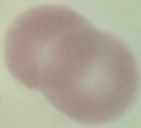
Another task frequently found when solving practical problems is the automatic separation of overlapping objects. Suppose we have an image of many round or oval objects, such the a microscope image of blood cells. If we want to count the number of cells, there are problems with cases such as in Figure 6, with two overlying blood cells. They must count not as one, but two.

Figure 6: Separating overlapping blood cells, shown in (a). Steps: (b) initial segmentation; (c) euclidean distance transform; and (d) correctly segmented image.

The input image is downloadable at:

http://siptoolbox.sourceforge.net/tutorial/images/cells.png

Start by reading the image and threshold it:

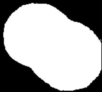
 a = gray_imread(’cells.png’);  // reads in grayscale
 imshow(a);
 b = im2bw(a, 0.9);
 imshow(b,2);

Figure 6 shows the result. We now calculate the distance transform of the inverse image:

 b = 1 - b;     // inverts image
 d = bwdist(b); // distance transform (euclidean distances)
 d = sqrt(d);   // square root of the values
 d = normal(d); // rescales to 0-1 range

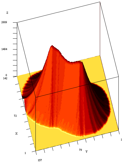
To understand the distance transform, we use a command from the ENRICO toolbox to make a nice 3D plot:

 set(gcf(), ’auto_clear’,’off’); //disables automatic clear
 [nrows, ncols] = size(d);
 figure(2); // use another window
 setcmap();        // chose the ’Hot’ colormap
 set(gcf(),’pixmap’,1);  // double-buffering mode (faster)
 shadesurf2(1:nrows, 1:ncols, d *200); // comp. the surface
 xset(’wshow’);  // shows the surface

You may click on the button ’3D Rot.’ to rotate the surface. The above commands render the distance transform as a surface (figure 6). The higher the surface, the greater the distance of the corresponding pixel to the image background. Note that the peaks of the distance transform are in the middle of each blob. The idea is to run Watershed segmentation [17] using those peaks as markers. For this, complement the distance transform so that the peaks become minima:

d = 1-d;

Apply a slight median filter [1] to eliminate spurious minima:

dm = mogrify(d,[’-median’,’2’]);

Force pixels that don’t belong to the objects to be at zero distance:

dm = dm .* b;

And finally perform watershed segmentation:

w = watershed(dm);
clf;
imshow(w, rand(10,3));  // use 10 colors at most

Variable ’w’ is an image with a unique number for each watershed region. The imshow with a random colormap displays each region with a unique arbitrary color. Note how the regions were correctly separated by watershed, except for the hardest cases. We can use this procedure for automatic counting objects in an image with many cells, and it’s robust to overlaps. This is specially useful to deal with bigger images at a large scale.

If the image had many cells, by the same procedure it would be straightforward to count the regions:

 n = maxi(w) - 1;   // subtract 1 for background

8 Conclusions

Scilab and SIP constitute a powerful and easy-to-use environment for rapid development of image processing solutions. The expressiveness of the Scilab interpreted language allows image manipulation in a natural way. Together with the SIP toolbox, we showed how simple it is to carry out complex operations such as the FFT, watershed segmentation, and multiscale skeletonization, in this environment.

As authors of the SIP Toolbox, we attest that the free software  model – an Open Source model [18] which is guaranteed to always remain free – has been essential to its development and success. First of all, the wide visibility of any free software easily sustains its development after once it is born. The feedback provided by direct contact with users and many co-developers also copes for the stability and usability of the toolbox. Furthermore, all the third-party packages used by SIP are Open Source: external libraries such as ImageMagick, Animal and OpenCV, as well as Scilab itself. This provides an excellent development environment, where any bugs in the third-party components may be reported directly to their authors, or even fixed by ourselves without bureaucracy. In addition, the community benefits a lot. Many scientists have replaced expensive proprietary software even big companies can’t afford. They also benefit from the sourcecode of many algorithms, by studying, evaluating and comparing them.

There is a clear demand in the Computer Vision community for software packages like SIP. Currently there is no other free software that provides easy scripting for image analysis together with the advanced techniques available in SIP. The number of supported file formats supersedes many proprietary software, such as Matlab. As a consequence, many people in universities and some industries have been using SIP, specially researchers and Image Processing students. The toolbox has reportedly been used in countries such as Germany, USA, Brazil, Greece, and France.

References

- [1] R. C. Gonzalez and R. E. Woods, Digital Image Processing. Reading, Massachusetts: Addison-Wesley, 1992.
- [2] R. Parker, Algorithms for image processing and computer vision. Wiley, 1997.
- [3] L. F. Costa and R. M. Cesar Jr., Shape Analysis and Classification, Theory and Practice. CRC Press, 2001.
- [4] S. Kimball and P. Mattis, “GIMP: GNU Image Manipulation Program.” http://www.gimp.org.
- [5] J. K. Osterhout, “Scripting languages: Higher-level programming for the 21st century,” IEEE Computer, no. 31, pp. 23–30, 1998.
- [6] Mathworks, Inc., “Matlab.” http://www.mathworks.com.
- [7] J. W. Eaton, “Octave.” http://www.octave.org.
- [8] Numerical Python community, “The numerical Python project.” http://www.pfdubois.com/numpy.
- [9] INRIA, “Scilab.” www.scilab.org.
- [10] R. Fabbri, “SIP: Scilab image processing toolbox.” http://siptoolbox.sourceforge.net.
- [11] J. Cristy, “ImageMagick.” www.imagemagick.org.
- [12] R. Fabbri, L. da F. Costa, J. C. Torelli, and O. M. Bruno, “2D euclidean distance transform algorithms: A comparative survey,” ACM Computing Surveys, vol. 40, no. 1, pp. 1–44, 2008.
- [13] R. Fabbri, “SIP development homepage.” http://siptoolbox.sourceforge.net/devel.
- [14] R. Fabbri, “Animal: An imaging library.” http://animal.sf.net.
- [15] L. F. Estrozi and L. F. Costa, “The scale space skeletonization homepage.” http://cyvision.if.sc.usp.br/msskeletons, 1999.
- [16] A. Falcao, L. F. Costa, and B. Da Cunha, “Multiscale skeletons by image foresting transform and its application to neuromorphometry,” Pattern Recognition, vol. 35, pp. 1571–1582, jul 2002.
- [17] P. Soille and L. Vincent, “Watersheds in digital spaces: An efficient algorithm based on imersion simmulations,” IEEE Trans. on Pattern Analysis and Machine Intelligence, vol. 13, no. 6, pp. 583–598, 1991.
- [18] E. S. Raymond, The Cathedral and the Bazaar: Musings on Linux and Open Source by an Accidental Revolutionary. Sebastopol, California: O’Reilly and Associates, 2001.