\field

D \authorlist\authorentry[wangzhe@cse.buaa.edu.cn]Zhe WANGnlabelA \authorentryKai HUmlabelA \authorentryBaolin YINnlabelA \affiliate[labelA]The authors are with the State Key Laboratory of Software Development Environment, the School of Computer Science and Engineering, Beihang University, Beijing, China. 912

An Improved Traffic Matrix Decomposition Method with Frequency-Domain Regularization

(2012)
keywords:
Traffic Matrix, Stable Principal Component Pursuit, Frequency-Domain Regularization, Iterative Algorithm.
titlenote: This work is supported by the National Natural Science Foundation of China (Nos. 61073013 and 90818024) and the Open Project of State Key Laboratory of Software Development Environment (No. SKLSDE-2012ZX-15).
{summary}

We propose a novel network traffic matrix decomposition method named Stable Principal Component Pursuit with Frequency-Domain Regularization (SPCP-FDR), which improves the Stable Principal Component Pursuit (SPCP) method by using a frequency-domain noise regularization function. An experiment demonstrates the feasibility of this new decomposition method.

1 Introduction

The network traffic matrix has been applied to many significant application problems such as capacity planning, traffic engineering and anomaly detection. A traffic matrix combines diverse traffic components with distinct temporal properties. Therefore, it is necessary to decompose them efficiently, and this problem is named traffic matrix structural analysis [1]. We presented the traffic matrix decomposition model in [2] and decomposed a traffic matrix into three sub-matrices, which is equivalent to the generalized Robust Principal Component Analysis (RPCA) problem [3]. The results in [2] were achieved by applying the Stable Principal Component Pursuit (SPCP) method in [3].

In this study, we improve the traffic matrix decomposition method by using frequency-domain regularization. This method is a variation of SPCP, and is named Stable Principal Component Pursuit with Frequency-Domain Regularization (SPCP-FDR). We design the numerical algorithm for SPCP-FDR, evaluate its decomposition results on the Abilene dataset [7], and show that SPCP-FDR achieves more rational traffic decompositions compared with SPCP.

2 Background

The standard RPCA problem is formally defined in [4]:

Problem 1 (Standard RPCA) Suppose that a known matrix Xm×n𝑋superscript𝑚𝑛X\in\mathbb{R}^{m\times n} is of the form A+E𝐴𝐸A+E, where A𝐴A and E𝐸E are unknown matrices. It is assumed that A𝐴A has a low rank and E𝐸E is sparse. The problem is to recover A𝐴A and E𝐸E.

In many applications, data matrices satisfying the assumptions in Problem 1 are polluted by dense noise with small magnitude. This leads to the generalized RPCA [3]:

Problem 2 (Generalized RPCA) Suppose that a known matrix Xm×n𝑋superscript𝑚𝑛X\in\mathbb{R}^{m\times n} is of the form A+E+N𝐴𝐸𝑁A+E+N, where A𝐴A, E𝐸E and N𝑁N are unknown matrices. It is assumed that A𝐴A has a low-rank, E𝐸E is sparse, and N𝑁N is an i.i.d. entry-wide noise matrix with small magnitude. The problem is to recover A𝐴A, E𝐸E and N𝑁N.

We refer RPCA as the generalized version as follows. Zhou et al. [3] proved that under surprising board conditions, for ”almost all” data matrix X𝑋X which is the sum of a low-rank matrix and a sparse matrix, and is corrupted by a dense noise matrix N𝑁N whose Frobenius norm NFδsubscriptnorm𝑁𝐹𝛿\|N\|_{F}\leq\delta (δ𝛿\delta is a positive constant), one could stably estimate A𝐴A and E𝐸E with high probability using this convex program:

minA,EA+λE1s.t.XA+EFδ,formulae-sequencesubscript𝐴𝐸subscriptnorm𝐴𝜆subscriptnorm𝐸1𝑠𝑡subscriptnorm𝑋𝐴𝐸𝐹𝛿\min_{A,E}\|A\|_{\ast}+\lambda\|E\|_{1}\ \ \ \ s.t.\|X-A+E\|_{F}\leq\delta, (1)

where λ𝜆\lambda is a positive parameter, \|\cdot\|_{\ast} and 1\|\cdot\|_{1} denote the matrix nuclear norm and the l1subscript𝑙1l_{1} norm, respectively. They named this method as Stable Principal Component Pursuit (SPCP), which needs to solve a time-consuming constrained program. Thus they turned to solve another similar unconstrained program instead (τ𝜏\tau is another positive parameter):

minA,Eτ(A+λE1)+12XAEF2.subscript𝐴𝐸𝜏subscriptnorm𝐴𝜆subscriptnorm𝐸112superscriptsubscriptnorm𝑋𝐴𝐸𝐹2\min_{A,E}\tau(\|A\|_{\ast}+\lambda\|E\|_{1})+\frac{1}{2}\|X-A-E\|_{F}^{2}. (2)

Suppose XT×P𝑋superscript𝑇𝑃X\in\mathbb{R}^{T\times P} is a traffic matrix, and each column XjTsubscript𝑋𝑗superscript𝑇X_{j}\in\mathbb{R}^{T} (1jP1𝑗𝑃1\leq j\leq P) is the traffic time-series of an Original-Destination (OD) flow. Following the traffic matrix decomposition model [2], X𝑋X is the sum of three sub-matrices: (1) The deterministic traffic matrix A𝐴A is a low-rank matrix, contributed by the periodic traffic changes in each OD flow; (2) The anomaly traffic matrix E𝐸E is a sparse matrix, but its nonzero entries may have large magnitudes; (3) The noise matrix N𝑁N is constituted of independent random variables with relatively small magnitudes, the entries in one column constitute a white noise vector, but those in different columns have distinct variances. In [2], we estimated the noise traffic variances {σj}j=1Psuperscriptsubscriptsubscript𝜎𝑗𝑗1𝑃\{\sigma_{j}\}_{j=1}^{P} of all the OD flows in X𝑋X, and divided Xjsubscript𝑋𝑗X_{j} by σjsubscript𝜎𝑗\sigma_{j} (1jP1𝑗𝑃1\leq j\leq P). This preprocessing normalizes random variables in N𝑁N, and preserves the rank of A𝐴A, as well as the sparsity of E𝐸E. Thus traffic matrix decomposition is equivalent to RPCA, and we only consider traffic matrices with unit noise traffic variance.

3 Stable Principal Component Pursuit with Frequency-Domain Regularization

Suppose ”\circledast” is a traffic matrix decomposition method, and NT×Psuperscript𝑁superscript𝑇𝑃N^{\circledast}\in\mathbb{R}^{T\times P} is the decomposed noise traffic matrix of X𝑋X by \circledast. In this letter, SPCP and SPCP-FDR are denoted as ”direct-product\odot” and ”direct-sum\oplus”, respectively. We consider the frequency-domain property of the decomposed noise traffic matrices. For each noise traffic time-series Njsubscriptsuperscript𝑁𝑗N^{\circledast}_{j} (the jlimit-from𝑗j-th column of Nsuperscript𝑁N^{\circledast}), αjTsubscript𝛼𝑗superscript𝑇\alpha_{j}\in\mathbb{C}^{T} denotes its Discrete Fourier Transform (DFT):

αj=WTNj=[W1W2WT]TNj,subscript𝛼𝑗superscript𝑊Tsubscriptsuperscript𝑁𝑗superscriptdelimited-[]subscript𝑊1subscript𝑊2subscript𝑊𝑇Tsubscriptsuperscript𝑁𝑗\alpha_{j}=W^{\textrm{T}}N^{\circledast}_{j}=\left[W_{1}\ W_{2}\ \cdots\ W_{T}\right]^{\textrm{T}}N^{\circledast}_{j}, (3)

where WT×T𝑊superscript𝑇𝑇W\in\mathbb{C}^{T\times T} is the discrete Fourier basis matrix. The tlimit-from𝑡t-th column vector WtTsubscript𝑊𝑡superscript𝑇W_{t}\in\mathbb{C}^{T} (1tT1𝑡𝑇1\leq t\leq T) is defined as:

Wt(k)=1Te2πiT(t1)(k1)k=1,2,,T.formulae-sequencesubscript𝑊𝑡𝑘1𝑇superscript𝑒2𝜋𝑖𝑇𝑡1𝑘1𝑘12𝑇W_{t}(k)=\frac{1}{\sqrt{T}}e^{-\frac{2\pi i}{T}(t-1)(k-1)}\ \ \ \ k=1,2,...,T. (4)

Njsubscriptsuperscript𝑁𝑗N^{\circledast}_{j}’s spectral density φjTsubscript𝜑𝑗superscript𝑇\varphi_{j}\in\mathbb{R}^{T} is defined as:

φj(t)=|αj(t)|2t=1,2,,T.formulae-sequencesubscript𝜑𝑗𝑡superscriptsubscript𝛼𝑗𝑡2𝑡12𝑇\varphi_{j}(t)=\left|\alpha_{j}(t)\right|^{2}\ \ \ \ t=1,2,...,T. (5)

As Njsubscriptsuperscript𝑁𝑗N^{\circledast}_{j} is a real signal, φj(t)=φj(Tt+2)subscript𝜑𝑗𝑡subscript𝜑𝑗𝑇𝑡2\varphi_{j}(t)=\varphi_{j}(T-t+2) for each position t[2,T]𝑡2𝑇t\in[2,T]\cap\mathbb{N}, and (Tt+2)𝑇𝑡2(T-t+2) is named the dual position of t𝑡t. The spectra φj(t)subscript𝜑𝑗𝑡\varphi_{j}(t) at positions close to 222 or T𝑇T describe Njsubscriptsuperscript𝑁𝑗N^{\circledast}_{j}’s power distributed in low-frequency domain; conversely, the spectra at positions close to (T2+1)𝑇21(\frac{T}{2}+1) indicate the high-frequency power. Furthermore, the spectral density ΦNTsubscriptΦsuperscript𝑁superscript𝑇\Phi_{N^{\circledast}}\in\mathbb{R}^{T} of Nsuperscript𝑁N^{\circledast} is defined as the entry-wise sum of all the noise traffic time-series’ spectral density:

ΦN(t)=j=1Pφj(t)t=1,2,,T.formulae-sequencesubscriptΦsuperscript𝑁𝑡superscriptsubscript𝑗1𝑃subscript𝜑𝑗𝑡𝑡12𝑇\Phi_{N^{\circledast}}(t)=\sum_{j=1}^{P}\varphi_{j}(t)\ \ \ \ t=1,2,...,T. (6)

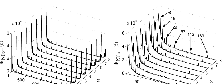
We compute the spectral density of eight noise traffic matrices N01N08similar-toNsuperscript01direct-productNsuperscript08direct-product\textrm{N}01^{\odot}\sim\textrm{N}08^{\odot} and display them in Fig. 1, which are independently decomposed from the eight Abilene [7] weekly traffic matrices X01X08similar-toX01X08\textrm{X}01\sim\textrm{X}08 by SPCP we adopted in [2]. In this dataset, P=121𝑃121P=121, T=2016𝑇2016T=2016, and the minimal time interval is 5 minutes. Thus for each noise traffic matrix N0xsuperscriptN0xdirect-product\textrm{N0x}^{\odot} (x{1,2,,8}x128\textrm{x}\in\{1,2,...,8\}), ΦN0x(t)subscriptΦsuperscriptN0xdirect-product𝑡\Phi_{\textrm{N0x}^{\odot}}(t) represents the power captured by periodic traffic with period 2016min(t1,2016t+2)5602016𝑡12016𝑡2560\frac{2016}{\min(t-1,2016-t+2)}\frac{5}{60} hour(s). We discover these two properties for the noise traffic matrices decomposed by SPCP: (1) The low-frequency spectra are generally much larger than the high-frequency spectra. This means that most energy of these noise traffic matrices is contributed by the low-frequency traffic patterns; (2) Quite a few low-frequency spectra have dramatically larger values than their neighbors (No. 8, 15, 29, 57, 113 and 169 spectra, as well as the spectra at dual positions, and their corresponding periods are 24, 12, 6, 3, 1.5 and 1 hour(s), respectively).
Refer to caption
Figure 1: The spectral density of N01N08similar-toNsuperscript01direct-productNsuperscript08direct-product\textrm{N}01^{\odot}\sim\textrm{N}08^{\odot} (left); For each noise traffic matrix, the first 200 positions of its spectral density are specially magnified (right), which describe the low-frequency power.

These properties match our assumptions of the noise traffic poorly. As each column of the noise traffic matrix is assumed as a white noise vector, if the noise traffic is exactly recovered by SPCP, the spectral density should show a flat distribution. We briefly explain the cause of this limitation. In most cases, the volume of a traffic matrix is mainly contributed by the deterministic traffic. The deterministic traffic changes slowly and shows typical diurnal pattern. Therefore, the spectral density of each OD flow presents unbalanced distribution: The low-frequency spectra usually have much larger values, and the spectra whose periods are the factors of 24 hours show strong peaks. The optimization problem (2) can be written in this equivalent form:

minA,E,NA+λE1+γNF2s.t.A+E+N=X,formulae-sequencesubscript𝐴𝐸𝑁subscriptnorm𝐴𝜆subscriptnorm𝐸1𝛾superscriptsubscriptnorm𝑁𝐹2𝑠𝑡𝐴𝐸𝑁𝑋\min_{A,E,N}\|A\|_{\ast}+\lambda\|E\|_{1}+\gamma\|N\|_{F}^{2}\ \ s.t.A+E+N=X, (7)

where γ=1/2τ𝛾12𝜏\gamma=1/2\tau, and the objective function for N𝑁N is the Frobenius norm. Thus problem (7) has no frequency-domain consideration on the noise traffic. With high probability, the noise traffic decomposed by SPCP inherits the unbalanced spectral density distribution of the OD flow traffic.

These discussions motivate us to replace NF2superscriptsubscriptnorm𝑁𝐹2\|N\|_{F}^{2} by a new objective function which focuses on N𝑁N’s frequency-domain property, and the new decomposed noise traffic should have more flat spectral density. We define the frequency-domain weight matrix C=diag(c1,,cT)𝐶diagsubscript𝑐1subscript𝑐𝑇C=\operatorname*{diag}(c_{1},...,c_{T}) satisfying:

ct>0,t=1,2,,T;t=1Tct2=T.formulae-sequencesubscript𝑐𝑡0formulae-sequence𝑡12𝑇superscriptsubscript𝑡1𝑇superscriptsubscript𝑐𝑡2𝑇c_{t}>0,\ t=1,2,...,T;\ \ \sum_{t=1}^{T}c_{t}^{2}=T. (8)

We propose the new traffic decomposition method called Stable Principal Component Pursuit with Frequency-Domain Regularization (SPCP-FDR). Compared with SPCP, SPCP-FDR adopts the same objective functions for the deterministic and the anomaly traffic, respectively; while CWTNFsubscriptnorm𝐶superscript𝑊T𝑁𝐹\|CW^{\textrm{T}}N\|_{F} is chosen as the new objective function for the noise traffic (C𝐶C’s design is presented in Section 4):

minA,E,NA+λE1+γCWTNF2s.t.A+E+N=X,formulae-sequencesubscript𝐴𝐸𝑁subscriptnorm𝐴𝜆subscriptnorm𝐸1𝛾superscriptsubscriptnorm𝐶superscript𝑊T𝑁𝐹2𝑠𝑡𝐴𝐸𝑁𝑋\min_{A,E,N}\|A\|_{\ast}+\lambda\|E\|_{1}+\gamma\|CW^{\textrm{T}}N\|_{F}^{2}\ \ s.t.A+E+N=X, (9)

where λ𝜆\lambda and γ𝛾\gamma are positive parameters balancing the three objective functions. We choose λ=1/max(T,P)𝜆1𝑇𝑃\lambda=1/\sqrt{\max(T,P)} because it is demonstrated as a proper choice in [4]. For the choice of γ𝛾\gamma, consider the simplest case: each column in N𝑁N is a standard Gaussian white noise. The DFT of one Gaussian white noise is also a Gaussian white noise, and it can be proved that 𝔼[CWTNF2]=𝔼[NF2]𝔼delimited-[]superscriptsubscriptnorm𝐶superscript𝑊T𝑁𝐹2𝔼delimited-[]superscriptsubscriptnorm𝑁𝐹2\mathbb{E}\left[\|CW^{\textrm{T}}N\|_{F}^{2}\right]=\mathbb{E}\left[\|N\|_{F}^{2}\right] (𝔼𝔼\mathbb{E} denotes expectation). Therefore, SPCP-FDR can be seen as an approximation of SPCP under the Gaussian white noise assumption. In [2], we choose τ=2log(TP)max(T,P)𝜏2𝑇𝑃𝑇𝑃\tau=\sqrt{2\log(TP)\max(T,P)} for problem (2). Thus in this study γ=1/2τ=1/(22log(TP)max(T,P))𝛾12𝜏122𝑇𝑃𝑇𝑃\gamma=1/2\tau=1/\left(2\sqrt{2\log(TP)\max(T,P)}\right).

4 Implementation Details

4.1 The Design of Frequency-Domain Weight Matrix

We design C𝐶C for decomposing the Abilene weekly traffic matrices (T=2016𝑇2016T=2016), and we believe that the key technologies are adaptable to other datasets with small modifications. Instinctively, it punishes the low-frequency spectra, especially for the spectra whose corresponding periods are the factors of 24 hours. Define the position set S1subscript𝑆1S_{1} as:

S1=S1aS1b;S1a={8,15,29,57,113,169};S1b={t|(Tt+2)S1a}.formulae-sequencesubscript𝑆1superscriptsubscript𝑆1𝑎superscriptsubscript𝑆1𝑏formulae-sequencesuperscriptsubscript𝑆1𝑎8152957113169superscriptsubscript𝑆1𝑏conditional-set𝑡𝑇𝑡2superscriptsubscript𝑆1𝑎\begin{split}&S_{1}=S_{1}^{a}\cup S_{1}^{b};\\ &S_{1}^{a}=\{8,15,29,57,113,169\};\ S_{1}^{b}=\{t\ |\ (T-t+2)\in S_{1}^{a}\}.\end{split}

S1bsuperscriptsubscript𝑆1𝑏S_{1}^{b} represents the dual positions of S1asuperscriptsubscript𝑆1𝑎S_{1}^{a}. We design {ct}t=1Tsuperscriptsubscriptsubscript𝑐𝑡𝑡1𝑇\{c_{t}\}_{t=1}^{T} as:

ct={β[v(t)+ρ]tS1βv(t)otherwise,subscript𝑐𝑡cases𝛽delimited-[]𝑣𝑡𝜌𝑡subscript𝑆1𝛽𝑣𝑡otherwisec_{t}=\begin{cases}\beta[v(t)+\rho]&t\in S_{1}\\ \beta v(t)&\textrm{otherwise}\end{cases}, (10)

where v(x)𝑣𝑥v(x) is a positive function in [1,T]1𝑇[1,T] satisfying v(x)=v(Tx+2)𝑣𝑥𝑣𝑇𝑥2v(x)=v(T-x+2) in [2,T]2𝑇[2,T]. Meanwhile, it decreases monotonically in [1,T2+1]1𝑇21[1,\frac{T}{2}+1]. ρ>0𝜌0\rho>0 is an additional penal parameter for the spectra correlated to S1subscript𝑆1S_{1}. β>0𝛽0\beta>0 is a scaling parameter. In this study, we choose

v(x)={4e(x1)200+1x[1,T2+1)4e(Tx+1)200+1x[T2+1,T]𝑣𝑥cases4superscript𝑒𝑥12001𝑥1𝑇214superscript𝑒𝑇𝑥12001𝑥𝑇21𝑇v(x)=\begin{cases}4e^{-\frac{(x-1)}{200}}+1&x\in[1,\frac{T}{2}+1)\\ 4e^{-\frac{(T-x+1)}{200}}+1&x\in[\frac{T}{2}+1,T]\end{cases} (11)

and ρ=2𝜌2\rho=2. At last, we get β=0.4832𝛽0.4832\beta=0.4832 from assumption (8) for this special choice of v(x)𝑣𝑥v(x) and ρ𝜌\rho.

4.2 The APG Algorithm for SPCP-FDR

The Accelerated Proximal Gradient (APG) algorithm for SPCP-FDR solves a relaxed approximation problem of (9):

minA,E,NF(A,E,N)=minA,E,Nμg(A,E,N)+f(A,E,N)g(A,E,N)A+λE1+γCWTNF2,f(A,E,N)12A+E+NXF2,formulae-sequencesubscript𝐴𝐸𝑁𝐹𝐴𝐸𝑁subscript𝐴𝐸𝑁𝜇𝑔𝐴𝐸𝑁𝑓𝐴𝐸𝑁𝑔𝐴𝐸𝑁subscriptdelimited-∥∥𝐴𝜆subscriptdelimited-∥∥𝐸1𝛾superscriptsubscriptdelimited-∥∥𝐶superscript𝑊T𝑁𝐹2𝑓𝐴𝐸𝑁12superscriptsubscriptdelimited-∥∥𝐴𝐸𝑁𝑋𝐹2\begin{split}&\min_{A,E,N}F(A,E,N)=\min_{A,E,N}\mu g(A,E,N)+f(A,E,N)\\ &g(A,E,N)\triangleq\|A\|_{\ast}+\lambda\|E\|_{1}+\gamma\|CW^{\textrm{T}}N\|_{F}^{2},\\ &f(A,E,N)\triangleq\frac{1}{2}\|A+E+N-X\|_{F}^{2},\end{split} (12)

where μ>0𝜇0\mu>0 is a parameter. As μ0𝜇0\mu\rightarrow 0, the solution to (12) approaches to the solution to (9). Not directly minimizing F(A,E,N)𝐹𝐴𝐸𝑁F(A,E,N), this algorithm minimizes a sequence of quadratic approximations Q(A,E,N,YA,YE,YN)𝑄𝐴𝐸𝑁superscript𝑌𝐴superscript𝑌𝐸superscript𝑌𝑁Q(A,E,N,Y^{A},Y^{E},Y^{N}) to F(A,E,N)𝐹𝐴𝐸𝑁F(A,E,N) at point (YA,YE,YN)superscript𝑌𝐴superscript𝑌𝐸superscript𝑌𝑁(Y^{A},Y^{E},Y^{N}) (renewed in each step):

Q(A,E,N,YA,YE,YN)μg(A,E,N)+f(YA,YE,YN)+f(YA,YE,YN),(A,E,N)(YA,YE,YN)+Lf2(A,E,N)(YA,YE,YN)F2,𝑄𝐴𝐸𝑁superscript𝑌𝐴superscript𝑌𝐸superscript𝑌𝑁𝜇𝑔𝐴𝐸𝑁𝑓superscript𝑌𝐴superscript𝑌𝐸superscript𝑌𝑁𝑓superscript𝑌𝐴superscript𝑌𝐸superscript𝑌𝑁𝐴𝐸𝑁superscript𝑌𝐴superscript𝑌𝐸superscript𝑌𝑁subscript𝐿𝑓2superscriptsubscriptdelimited-∥∥𝐴𝐸𝑁superscript𝑌𝐴superscript𝑌𝐸superscript𝑌𝑁𝐹2\begin{split}&Q(A,E,N,Y^{A},Y^{E},Y^{N})\\ \triangleq&\mu g(A,E,N)+f(Y^{A},Y^{E},Y^{N})+\\ &\langle\nabla f(Y^{A},Y^{E},Y^{N}),(A,E,N)-(Y^{A},Y^{E},Y^{N})\rangle+\\ &\frac{L_{f}}{2}\|(A,E,N)-(Y^{A},Y^{E},Y^{N})\|_{F}^{2},\end{split} (13)

where the Lipschitz constant Lf=3subscript𝐿𝑓3L_{f}=3. It can be derived that:

minA,E,NQ(A,E,N,YA,YE,YN)=minALf2AGAF2+μA+minELf2EGEF2+μλE1+minNLf2NGNF2+μγCWTNF2+constant,subscript𝐴𝐸𝑁𝑄𝐴𝐸𝑁superscript𝑌𝐴superscript𝑌𝐸superscript𝑌𝑁subscript𝐴subscript𝐿𝑓2superscriptsubscriptdelimited-∥∥𝐴superscript𝐺𝐴𝐹2𝜇subscriptdelimited-∥∥𝐴subscript𝐸subscript𝐿𝑓2superscriptsubscriptdelimited-∥∥𝐸superscript𝐺𝐸𝐹2𝜇𝜆subscriptdelimited-∥∥𝐸1subscript𝑁subscript𝐿𝑓2superscriptsubscriptdelimited-∥∥𝑁superscript𝐺𝑁𝐹2𝜇𝛾superscriptsubscriptdelimited-∥∥𝐶superscript𝑊T𝑁𝐹2constant\begin{split}&\min_{A,E,N}Q(A,E,N,Y^{A},Y^{E},Y^{N})\\ =&\min_{A}\frac{L_{f}}{2}\|A-G^{A}\|_{F}^{2}+\mu\|A\|_{\ast}+\\ &\min_{E}\frac{L_{f}}{2}\|E-G^{E}\|_{F}^{2}+\mu\lambda\|E\|_{1}+\\ &\min_{N}\frac{L_{f}}{2}\|N-G^{N}\|_{F}^{2}+\mu\gamma\|CW^{\textrm{T}}N\|_{F}^{2}+\textrm{constant},\end{split} (14)

where

G=Y1Lf(YA+YE+YNX),{A,E,N}.formulae-sequencesuperscript𝐺superscript𝑌1subscript𝐿𝑓superscript𝑌𝐴superscript𝑌𝐸superscript𝑌𝑁𝑋𝐴𝐸𝑁G^{\square}=Y^{\square}-\frac{1}{L_{f}}(Y^{A}+Y^{E}+Y^{N}-X),\ \ \square\in\{A,E,N\}. (15)

Problem (LABEL:APG_subproblem) splits into three independent optimization problems, and the first two (for A𝐴A and E𝐸E) are well studied [5]. We give the solution to the third problem by derivation:

N=Lf[LfIT×T+2μγWC2WT]1GN.𝑁subscript𝐿𝑓superscriptdelimited-[]subscript𝐿𝑓subscript𝐼𝑇𝑇2𝜇𝛾𝑊superscript𝐶2superscript𝑊T1superscript𝐺𝑁N=L_{f}\left[L_{f}I_{T\times T}+2\mu\gamma WC^{2}W^{\textrm{T}}\right]^{-1}G^{N}. (16)

Following the main idea in [5], we present the APG algorithm for the SPCP-FDR method in Algorithm 1. This algorithm has the O(1/k2)𝑂1superscript𝑘2O(1/k^{2}) convergence rate. Because the proof is very close to Theorem 2.1 in [5] and Theorem 4.4 in [6], we omit it and directly summarize this result:

Theorem 1 Let F(A,E,N)=μ¯g(A,E,N)+f(A,E,N)𝐹𝐴𝐸𝑁¯𝜇𝑔𝐴𝐸𝑁𝑓𝐴𝐸𝑁F(A,E,N)=\overline{\mu}g(A,E,N)+f(A,E,N). Then for all k>k0log(μ0μ¯)/log(1η)𝑘subscript𝑘0subscript𝜇0¯𝜇1𝜂k>k_{0}\triangleq\left\lceil\log\left(\frac{\mu_{0}}{\overline{\mu}}\right)/\log\left(\frac{1}{\eta}\right)\right\rceil, we have

F(Xk)F(X)6Xk0XF2/(kk0+1)2,𝐹subscript𝑋𝑘𝐹superscript𝑋6superscriptsubscriptnormsubscript𝑋subscript𝑘0superscript𝑋𝐹2superscript𝑘subscript𝑘012F(X_{k})-F(X^{\ast})\leq 6\|X_{k_{0}}-X^{\ast}\|_{F}^{2}/(k-k_{0}+1)^{2}, (17)

where Xk=(Ak,Ek,Nk)subscript𝑋𝑘subscript𝐴𝑘subscript𝐸𝑘subscript𝑁𝑘X_{k}=(A_{k},E_{k},N_{k}) is defined in Algorithm 1, and X=(A,E,N)superscript𝑋superscript𝐴superscript𝐸superscript𝑁X^{\ast}=(A^{\ast},E^{\ast},N^{\ast}) is a solution to (12) when μ=μ¯𝜇¯𝜇\mu=\overline{\mu}. Notice that in this study Lf=3subscript𝐿𝑓3L_{f}=3, while in [5] it equals to 2.

Algorithm 1 The APG Algorithm for SPCP-FDR

Input: traffic matrix XT×P𝑋superscript𝑇𝑃X\in\mathbb{R}^{T\times P} with unit noise variance.

Initialization: A0=A1=E0=E1=N0=N1=0T×Psubscript𝐴0subscript𝐴1subscript𝐸0subscript𝐸1subscript𝑁0subscript𝑁1superscript0𝑇𝑃A_{0}=A_{-1}=E_{0}=E_{-1}=N_{0}=N_{-1}=\textbf{0}^{T\times P}; t0=t1=1subscript𝑡0subscript𝑡11t_{0}=t_{-1}=1; μ0=0.99X2subscript𝜇00.99subscriptnorm𝑋2\mu_{0}=0.99\|X\|_{2}; μ¯=105μ0¯𝜇superscript105subscript𝜇0\overline{\mu}=10^{-5}\mu_{0}; k=0𝑘0k=0.

η=0.9𝜂0.9\eta=0.9; Lf=3subscript𝐿𝑓3L_{f}=3; λ=1/max(T,P)𝜆1𝑇𝑃\lambda=1/\sqrt{\max(T,P)}; γ=1/(22log(TP)max(T,P))𝛾122𝑇𝑃𝑇𝑃\gamma=1/\left(2\sqrt{2\log(TP)\max(T,P)}\right).

While  not converged do

YkA=Ak+tk11tk(AkAk1)superscriptsubscript𝑌𝑘𝐴subscript𝐴𝑘subscript𝑡𝑘11subscript𝑡𝑘subscript𝐴𝑘subscript𝐴𝑘1Y_{k}^{A}=A_{k}+\frac{t_{k-1}-1}{t_{k}}(A_{k}-A_{k-1}); YkE=Ek+tk11tk(EkEk1)superscriptsubscript𝑌𝑘𝐸subscript𝐸𝑘subscript𝑡𝑘11subscript𝑡𝑘subscript𝐸𝑘subscript𝐸𝑘1Y_{k}^{E}=E_{k}+\frac{t_{k-1}-1}{t_{k}}(E_{k}-E_{k-1});

YkN=Nk+tk11tk(NkNk1)superscriptsubscript𝑌𝑘𝑁subscript𝑁𝑘subscript𝑡𝑘11subscript𝑡𝑘subscript𝑁𝑘subscript𝑁𝑘1Y_{k}^{N}=N_{k}+\frac{t_{k-1}-1}{t_{k}}(N_{k}-N_{k-1});

Gk=Yk1Lf(YkA+YkE+YkNX)subscriptsuperscript𝐺𝑘subscriptsuperscript𝑌𝑘1subscript𝐿𝑓subscriptsuperscript𝑌𝐴𝑘subscriptsuperscript𝑌𝐸𝑘subscriptsuperscript𝑌𝑁𝑘𝑋G^{\square}_{k}=Y^{\square}_{k}-\frac{1}{L_{f}}(Y^{A}_{k}+Y^{E}_{k}+Y^{N}_{k}-X), {A,E,N}𝐴𝐸𝑁\square\in\{A,E,N\};

(U,S,V)=svd[GkA]𝑈𝑆𝑉svddelimited-[]superscriptsubscript𝐺𝑘𝐴(U,S,V)=\mathrm{svd}\left[G_{k}^{A}\right];  //svd[]svddelimited-[]\mathrm{svd}[\cdot] denotes singular value decomposition.

Ak+1=U𝒮μkLf[S]VTsubscript𝐴𝑘1𝑈subscript𝒮subscript𝜇𝑘subscript𝐿𝑓delimited-[]𝑆superscript𝑉TA_{k+1}=U\mathcal{S}_{\frac{\mu_{k}}{L_{f}}}\left[S\right]V^{\textrm{T}}; Ek+1=𝒮λμkLf[GkE]subscript𝐸𝑘1subscript𝒮𝜆subscript𝜇𝑘subscript𝐿𝑓delimited-[]superscriptsubscript𝐺𝑘𝐸E_{k+1}=\mathcal{S}_{\frac{\lambda\mu_{k}}{L_{f}}}\left[G_{k}^{E}\right];

//𝒮ϵ[]subscript𝒮italic-ϵdelimited-[]\mathcal{S}_{\epsilon}[\cdot] denotes soft-thresholding operator with threshold ϵ>0italic-ϵ0\epsilon>0.

Nk+1=Lf[LfIT×T+2μkγWC2WT]1GkNsubscript𝑁𝑘1subscript𝐿𝑓superscriptdelimited-[]subscript𝐿𝑓subscript𝐼𝑇𝑇2subscript𝜇𝑘𝛾𝑊superscript𝐶2superscript𝑊T1superscriptsubscript𝐺𝑘𝑁N_{k+1}=L_{f}\left[L_{f}I_{T\times T}+2\mu_{k}\gamma WC^{2}W^{\textrm{T}}\right]^{-1}G_{k}^{N};

tk+1=(1+4tk2+1)/2subscript𝑡𝑘114superscriptsubscript𝑡𝑘212t_{k+1}=(1+\sqrt{4t_{k}^{2}+1})/2; μk+1=max(ημk,μ¯)subscript𝜇𝑘1𝜂subscript𝜇𝑘¯𝜇\mu_{k+1}=\max(\eta\mu_{k},\overline{\mu}); k=k+1𝑘𝑘1k=k+1.

End while

Output: A=Ak𝐴subscript𝐴𝑘A=A_{k}; E=Ek𝐸subscript𝐸𝑘E=E_{k}; N=Ek𝑁subscript𝐸𝑘N=E_{k}.

5 Experiment Results

Refer to caption
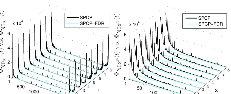
Figure 2: The spectral density of N01N08similar-toNsuperscript01direct-sumNsuperscript08direct-sum\textrm{N}01^{\oplus}\sim\textrm{N}08^{\oplus} decomposed by SPCP-FDR, compared with the spectral density of N01N08similar-toNsuperscript01direct-productNsuperscript08direct-product\textrm{N}01^{\odot}\sim\textrm{N}08^{\odot} decomposed by SPCP (left); For each matrix, the first 200 positions of its spectral density are specially magnified (right), which describe the low-frequency power.
Table 1: A comparison between SPCP and SPCP-FDR on the decomposed deterministic traffic matrices.
Traffic matrix rank(X0x)X0x(\textrm{X}0\textrm{x}) rank(A0x)A0superscriptxdirect-product(\textrm{A}0\textrm{x}^{\odot}) rank(A0x)A0superscriptxdirect-sum(\textrm{A}0\textrm{x}^{\oplus}) A0xFA0xFsubscriptnormA0superscriptxdirect-sum𝐹subscriptnormA0superscriptxdirect-product𝐹\frac{\|\textrm{A}0\textrm{x}^{\oplus}\|_{F}}{\|\textrm{A}0\textrm{x}^{\odot}\|_{F}}
X01(x=1)X01x1\textrm{X01}\ (\textrm{x}=1) 121 10 19 1.0158
X02(x=2)X02x2\textrm{X02}\ (\textrm{x}=2) 121 11 22 1.0171
X03(x=3)X03x3\textrm{X03}\ (\textrm{x}=3) 121 12 20 1.0283
X04(x=4)X04x4\textrm{X04}\ (\textrm{x}=4) 121 11 18 1.0145
X05(x=5)X05x5\textrm{X05}\ (\textrm{x}=5) 121 10 19 1.0148
X06(x=6)X06x6\textrm{X06}\ (\textrm{x}=6) 121 10 22 1.0162
X07(x=7)X07x7\textrm{X07}\ (\textrm{x}=7) 121 13 24 1.0210
X08(x=8)X08x8\textrm{X08}\ (\textrm{x}=8) 121 12 23 1.0182

We evaluate the SPCP-FDR method by using the Abilene traffic matrices X01X08similar-toX01X08\textrm{X}01\sim\textrm{X}08. For each x{1,,8}x18\textrm{x}\in\{1,...,8\}, suppose X0xX0x\textrm{X}0\textrm{x} is decomposed as {A0x,E0x,N0x}A0superscriptxdirect-sumE0superscriptxdirect-sumN0superscriptxdirect-sum\{\textrm{A}0\textrm{x}^{\oplus},\textrm{E}0\textrm{x}^{\oplus},\textrm{N}0\textrm{x}^{\oplus}\} and {A0x,E0x,N0x}A0superscriptxdirect-productE0superscriptxdirect-productN0superscriptxdirect-product\{\textrm{A}0\textrm{x}^{\odot},\textrm{E}0\textrm{x}^{\odot},\textrm{N}0\textrm{x}^{\odot}\} by SPCP-FDR and SPCP, respectively.

Figure 2 compares the spectral density of the noise traffic matrices N01N08similar-toNsuperscript01direct-sumNsuperscript08direct-sum\textrm{N}01^{\oplus}\sim\textrm{N}08^{\oplus} (blue) and N01N08similar-toNsuperscript01direct-productNsuperscript08direct-product\textrm{N}01^{\odot}\sim\textrm{N}08^{\odot} (black). For each x{1,,8}x18\textrm{x}\in\{1,...,8\}, N0xsuperscriptN0xdirect-sum\textrm{N0x}^{\oplus} has more flat spectral density distribution than N0xsuperscriptN0xdirect-product\textrm{N0x}^{\odot}. As we further regularize noise traffic’s spectra whose positions lie in S1subscript𝑆1S_{1}, their magnitudes dramatically decline. Therefore, for the new decompositions of X01X08similar-toX01X08\textrm{X}01\sim\textrm{X}08 by SPCP-FDR, most low-frequency traffic pattern is efficiently eliminated from the resulting noise traffic matrices N01N08similar-toNsuperscript01direct-sumNsuperscript08direct-sum\textrm{N}01^{\oplus}\sim\textrm{N}08^{\oplus}. Table 1 compares the deterministic traffic matrices A01A08similar-toAsuperscript01direct-sumAsuperscript08direct-sum\textrm{A}01^{\oplus}\sim\textrm{A}08^{\oplus} and A01A08similar-toAsuperscript01direct-productAsuperscript08direct-product\textrm{A}01^{\odot}\sim\textrm{A}08^{\odot}. The ranks of A01A08similar-toAsuperscript01direct-sumAsuperscript08direct-sum\textrm{A}01^{\oplus}\sim\textrm{A}08^{\oplus} decomposed by SPCP-FDR are nearly twice as those decomposed by SPCP. However, as all these values do not exceed 24 and the original traffic matrices’ ranks are 121, A01A08similar-toAsuperscript01direct-sumAsuperscript08direct-sum\textrm{A}01^{\oplus}\sim\textrm{A}08^{\oplus} still satisfy the low-rank characteristic. For each x{1,,8}x18\textrm{x}\in\{1,...,8\}, the Frobenius norm of A0xA0superscriptxdirect-sum\textrm{A}0\textrm{x}^{\oplus} is a little larger than that of A0xA0superscriptxdirect-product\textrm{A}0\textrm{x}^{\odot}, and it can be explained that most low-frequency traffic pattern eliminated from the noise traffic is added to the deterministic traffic.

Refer to caption
Figure 3: A comparison between SPCP and SPCP-FDR on the absolute Pearson correlation coefficients (between the deterministic traffic time-series and the noise traffic time-series of each OD flow) of X01X01\textrm{X}01.
Refer to caption
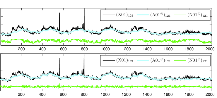
Figure 4: A comparison between SPCP and SPCP-FDR on the decomposition result of OD flow (X01)121subscriptX01121(\textrm{X}01)_{121}. Upper panel: the deterministic and the noise traffic time-series decomposed by SPCP; Bottom panel: the deterministic and the noise traffic time-series decomposed by SPCP-FDR.

As a case study, we analyze the decomposition result of X01X01\textrm{X}01 in detail. For each OD flow (X01)jsubscriptX01𝑗(\textrm{X}01)_{j} (1j1211𝑗1211\leq j\leq 121), compute the absolute Pearson correlation coefficient between (A01)jsubscriptAsuperscript01direct-sum𝑗(\textrm{A}01^{\oplus})_{j} and (N01)jsubscriptNsuperscript01direct-sum𝑗(\textrm{N}01^{\oplus})_{j}, and the coefficient between (A01)jsubscriptAsuperscript01direct-product𝑗(\textrm{A}01^{\odot})_{j} and (N01)jsubscriptNsuperscript01direct-product𝑗(\textrm{N}01^{\odot})_{j}. Figure 3 displays these coefficients arranged by flow ID. This is a proper metric of the cross-correlation and it should be as small as possible. For most OD flows in X01X01\textrm{X}01, compared with SPCP, SPCP-FDR’s absolute Pearson correlation coefficients show significant decline. Actually, X02X08similar-toX02X08\textrm{X}02\sim\textrm{X}08 show quite similar results. Thus SPCP-FDR could efficiently reduce this cross-correlation. Figure 4 compares SPCP-FDR with SPCP on decomposition result of the No. 121 OD flow, which produces the largest volume in X01X01\textrm{X}01. Instinctively, the noise traffic time-series (N01)121subscriptNsuperscript01direct-product121(\textrm{N}01^{\odot})_{121} contains a distinct diurnal trend, which should be classified as the deterministic traffic better. By contrast, (N01)121subscriptNsuperscript01direct-sum121(\textrm{N}01^{\oplus})_{121} presents a more stable temporal pattern. Thus SPCP-FDR gives a more rational decomposition for this flow.

6 Conclusions

This letter presents a novel traffic matrix decomposition method named SPCP-FDR, which improves SPCP by using frequency-domain regularization. We propose an APG algorithm for SPCP-FDR, its convergence rate is O(1/k2)𝑂1superscript𝑘2O(1/k^{2}), and demonstrate it on a real-world dataset. SPCP-FDR efficiently eliminates the low-frequency periodic traffic from the noise traffic, maintains deterministic traffic’s low-rank property, and shows lower cross-correlation between these two kinds of traffic than SPCP. Therefore, SPCP-FDR achieves more rational traffic decompositions.

References

  • [1] A. Lakhina, K. Papagiannaki, M. Crovella, C. Diot, E. D. Kolaczyk, and N. Taft. Structural analysis of network traffic flows. SIGMETRICS Perform. Eval. Rev. vol. 32, no. 1, pp. 61-72, June 2004.
  • [2] Z. Wang, K. Hu, K. Xu, B. Yin and X. Dong. Structural Analysis of Network Traffic Matrix via Relaxed Principal Component Pursuit. Computer Networks, vol. 56, no. 7, pp. 2049-2067, 2012.
  • [3] Z. Zhou, X. Li, J. Wright, E. Candes, and Y. Ma. Stable principal component pursuit. In Proc. IEEE ISIT 2010.
  • [4] E. Candes, X. Li, Y. Ma, and J. Wright. Robust principal component analysis? Journal of the ACM. vol. 58, no. 3, pp. 1-37, 2011.
  • [5] Z. Lin, A. Ganesh, J. Wright, L. Wu, M. Chen and Y. Ma. Fast convex optimization algorithms for exact recovery of a corrupted low-rank matrix. In Proc. IEEE CAMSAP 2009.
  • [6] A. Beck and M. Teboulle. A fast iterative shrinkage-thresholding algorithm for linear inverse problems. SIAM Journal on Imaging Sciences, vol. 2, no. 1, pp. 183-202, 2009.
  • [7] Abilene dataset: http://www.cs.utexas.edu/yzhang/research/AbileneTM/
\profile