Parameter Appendix

Bo Tan, John Thompson

This is a support document which describes the properties of the cable and parameters of the formulas in [1]. The cable parameters help the reader build powerline channel according to the transmission line theory. The document also presents the parameters which describe the distribution of the number of path, path magnitude, path interval and the cable loss feature of the powerline channel. By using the parameters in this document, readers can model the powerline channel according to the methodology proposed in [1].

1 Cable Property

Figure. 1 shows the structure of a power cable which is used in [2], Table 1 and Table 2 show the geometric parameters and the electromagnetic parameters of NAYY150 and NAYY35 cables. The insulator between conductors is PVC. When feeding signals into two adjacent conductors, most of the electric field is concentrated between these two conductors. The lumped parameters of the cable can be calculated by the geometric dimensions and material electrical properties.
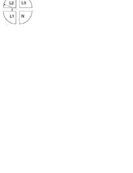
Refer to caption
Figure 1: The Cross-Section of a Four Conductor Power Cable, with three live connections (L1, L2 and L3) and one neutral connection (N). The scalar aπ‘Ža represents the space between two adjacent conductors which is filled by PVC. Scalar rπ‘Ÿr is the radius from geometry center to the outer edge of the conductor.
Table 1: Cable Geometry Properties
NAYY150 (mm) NAYY35 (mm)
a 1.8 1.2
r 6.9099 5.9161
Table 2: Cable Electrical Properties
Conductivity of Cooper ΞΊπœ…\kappa 58Γ—10658superscript10658\times 10^{6} S/m
Dissipation of PVC tanδ𝛿\delta 0.025
Relative permittivity of PVC Ξ΅rsubscriptπœ€π‘Ÿ\varepsilon_{r} 4
Free space permittivity Ξ΅0subscriptπœ€0\varepsilon_{0} 8.5419Γ—10βˆ’128.5419superscript10128.5419\times 10^{-12} F/m
Relative permeability of Cooper ΞΌrsubscriptπœ‡π‘Ÿ\mu_{r} 1
Free space permeability ΞΌ0subscriptπœ‡0\mu_{0} 1.2566Γ—10βˆ’61.2566superscript1061.2566\times 10^{-6} ΞΌ [H/m]

The lumped parameters such as capacitance (C𝐢C), inductance (L𝐿L), resistance (R𝑅R) and conductance (G𝐺G) per unit length can be calculated by applying the parameters in Table 1 and 2 to equation (1) to (4).

C𝐢\displaystyle C =\displaystyle= Ξ΅0​Ρr​rasubscriptπœ€0subscriptπœ€π‘Ÿπ‘Ÿπ‘Ž\displaystyle\varepsilon_{0}\varepsilon_{r}\dfrac{r}{a} (1)
L𝐿\displaystyle L =\displaystyle= ΞΌ0​μr​rasubscriptπœ‡0subscriptπœ‡π‘Ÿπ‘Ÿπ‘Ž\displaystyle\mu_{0}\mu_{r}\dfrac{r}{a} (2)
R𝑅\displaystyle R =\displaystyle= π​μ0κ​r2​fπœ‹subscriptπœ‡0πœ…superscriptπ‘Ÿ2𝑓\displaystyle\sqrt{\dfrac{\pi\mu_{0}}{\kappa r^{2}}f} (3)
G𝐺\displaystyle G =\displaystyle= 2​π​f​C​tan​δ2πœ‹π‘“πΆtan𝛿\displaystyle 2\pi fC\textrm{tan}\delta (4)

where, f𝑓f in equation (3) and (4) denotes the frequency with Hz as unit.

2 Parameters for Number of Paths Distribution

The number of the paths for the channel of the i𝑖ith Class and the kπ‘˜kth Cluster can be described by equation (7) in [1] which is a Gaussian distribution:

Ni,k=[𝒩​(ΞΌi,k,Οƒi,k2)]subscriptπ‘π‘–π‘˜delimited-[]𝒩subscriptπœ‡π‘–π‘˜subscriptsuperscript𝜎2π‘–π‘˜N_{i,k}=\left[\mathcal{N}(\mu_{i,k},\sigma^{2}_{i,k})\right] (5)

where [β‹…]delimited-[]β‹…\left[\cdot\right] means to round towards the nearest integer, parameters ΞΌi,ksubscriptπœ‡π‘–π‘˜\mu_{i,k} and Οƒi,k2subscriptsuperscript𝜎2π‘–π‘˜\sigma^{2}_{i,k} are the expectation and standard deviation of the Gaussian distribution. The value ΞΌπœ‡\mu and ΟƒπœŽ\sigma in each Class increase as power function of Cluster Index. The Power function can be written as:

ΞΌi,k=pi​1​kpi​2+pi​3subscriptπœ‡π‘–π‘˜subscript𝑝𝑖1superscriptπ‘˜subscript𝑝𝑖2subscript𝑝𝑖3\mu_{i,k}=p_{i1}k^{p_{i2}}+p_{i3} (6)
Οƒi,k2=qi​1​kqi​2+qi​3subscriptsuperscript𝜎2π‘–π‘˜subscriptπ‘žπ‘–1superscriptπ‘˜subscriptπ‘žπ‘–2subscriptπ‘žπ‘–3\sigma^{2}_{i,k}=q_{i1}k^{q_{i2}}+q_{i3} (7)

The parameters pi​1subscript𝑝𝑖1p_{i1}, pi​2subscript𝑝𝑖2p_{i2}, pi​3subscript𝑝𝑖3p_{i3}, qi​1subscriptπ‘žπ‘–1q_{i1}, qi​2subscriptπ‘žπ‘–2q_{i2} and qi​3subscriptπ‘žπ‘–3q_{i3} are shown in Table 3:

Table 3: Parameters for the Path Number distributions
i=2 pi​1=1.623subscript𝑝𝑖11.623p_{i1}=1.623 pi​2=0.08596subscript𝑝𝑖20.08596p_{i2}=0.08596 pi​3=0subscript𝑝𝑖30p_{i3}=0
qi​1=βˆ’0.3818subscriptπ‘žπ‘–10.3818q_{i1}=-0.3818 qi​2=βˆ’0.8461subscriptπ‘žπ‘–20.8461q_{i2}=-0.8461 qi​3=1.592subscriptπ‘žπ‘–31.592q_{i3}=1.592
i=3 pi​1=3.913subscript𝑝𝑖13.913p_{i1}=3.913 pi​2=0.0968subscript𝑝𝑖20.0968p_{i2}=0.0968 pi​3=0subscript𝑝𝑖30p_{i3}=0
qi​1=βˆ’0.005983subscriptπ‘žπ‘–10.005983q_{i1}=-0.005983 qi​2=1.033subscriptπ‘žπ‘–21.033q_{i2}=1.033 qi​3=1.783subscriptπ‘žπ‘–31.783q_{i3}=1.783
i=4 pi​1=6.169subscript𝑝𝑖16.169p_{i1}=6.169 pi​2=0.09686subscript𝑝𝑖20.09686p_{i2}=0.09686 pi​3=0subscript𝑝𝑖30p_{i3}=0
qi​1=βˆ’0.4401subscriptπ‘žπ‘–10.4401q_{i1}=-0.4401 qi​2=βˆ’0.6989subscriptπ‘žπ‘–20.6989q_{i2}=-0.6989 qi​3=2.007subscriptπ‘žπ‘–32.007q_{i3}=2.007
i=5 pi​1=8.684subscript𝑝𝑖18.684p_{i1}=8.684 pi​2=0.1688subscript𝑝𝑖20.1688p_{i2}=0.1688 pi​3=0subscript𝑝𝑖30p_{i3}=0
qi​1=βˆ’8.725subscriptπ‘žπ‘–18.725q_{i1}=-8.725 qi​2=βˆ’0.06764subscriptπ‘žπ‘–20.06764q_{i2}=-0.06764 qi​3=10.98subscriptπ‘žπ‘–310.98q_{i3}=10.98

3 Parameters for Magnitude Distribution

3.1 First Arrival Path

For the channels in a particular Class, the magnitude of the first arrival path of the i𝑖ith Class follows a double exponential decay distribution with the increase of the Cluster Index kπ‘˜k. In [1], equation (8) is used to describe the double exponential decay which can be written as:

Ii,k=aiM​ebiM​k+ciM​ediM​ksubscriptπΌπ‘–π‘˜superscriptsubscriptπ‘Žπ‘–π‘€superscript𝑒superscriptsubscriptπ‘π‘–π‘€π‘˜superscriptsubscript𝑐𝑖𝑀superscript𝑒superscriptsubscriptπ‘‘π‘–π‘€π‘˜I_{i,k}=a_{i}^{M}e^{b_{i}^{M}k}+c_{i}^{M}e^{d_{i}^{M}k} (8)

where aiMsuperscriptsubscriptπ‘Žπ‘–π‘€a_{i}^{M}, biMsuperscriptsubscript𝑏𝑖𝑀b_{i}^{M}, ciMsuperscriptsubscript𝑐𝑖𝑀c_{i}^{M} and diMsuperscriptsubscript𝑑𝑖𝑀d_{i}^{M} are the double exponential parameters, and are shown in Table 4:

Table 4: Parameters for the First Arrival Path Magnitude distribution
i=1 aiM=0.4815superscriptsubscriptπ‘Žπ‘–π‘€0.4815a_{i}^{M}=0.4815 biM=βˆ’0.0821superscriptsubscript𝑏𝑖𝑀0.0821b_{i}^{M}=-0.0821 ciM=0.4103superscriptsubscript𝑐𝑖𝑀0.4103c_{i}^{M}=0.4103 diM=βˆ’0.02408superscriptsubscript𝑑𝑖𝑀0.02408d_{i}^{M}=-0.02408
i=2 aiM=0.2601superscriptsubscriptπ‘Žπ‘–π‘€0.2601a_{i}^{M}=0.2601 biM=βˆ’0.1214superscriptsubscript𝑏𝑖𝑀0.1214b_{i}^{M}=-0.1214 ciM=0.4948superscriptsubscript𝑐𝑖𝑀0.4948c_{i}^{M}=0.4948 diM=βˆ’0.03241superscriptsubscript𝑑𝑖𝑀0.03241d_{i}^{M}=-0.03241
i=3 aiM=0.1841superscriptsubscriptπ‘Žπ‘–π‘€0.1841a_{i}^{M}=0.1841 biM=βˆ’0.1246superscriptsubscript𝑏𝑖𝑀0.1246b_{i}^{M}=-0.1246 ciM=0.3628superscriptsubscript𝑐𝑖𝑀0.3628c_{i}^{M}=0.3628 diM=βˆ’0.03334superscriptsubscript𝑑𝑖𝑀0.03334d_{i}^{M}=-0.03334
i=4 aiM=0.1221superscriptsubscriptπ‘Žπ‘–π‘€0.1221a_{i}^{M}=0.1221 biM=βˆ’0.1515superscriptsubscript𝑏𝑖𝑀0.1515b_{i}^{M}=-0.1515 ciM=0.2736superscriptsubscript𝑐𝑖𝑀0.2736c_{i}^{M}=0.2736 diM=βˆ’0.03445superscriptsubscript𝑑𝑖𝑀0.03445d_{i}^{M}=-0.03445
i=5 aiM=0.1721superscriptsubscriptπ‘Žπ‘–π‘€0.1721a_{i}^{M}=0.1721 biM=βˆ’0.1517superscriptsubscript𝑏𝑖𝑀0.1517b_{i}^{M}=-0.1517 ciM=0.0905superscriptsubscript𝑐𝑖𝑀0.0905c_{i}^{M}=0.0905 diM=βˆ’0.01979superscriptsubscript𝑑𝑖𝑀0.01979d_{i}^{M}=-0.01979

3.2 Other paths

The magnitude of the other paths are dependent on the arrival time of the path. The decay profile with the time sampling index can be also demonstrated by the double exponential function which is also can be seen in [1] as equation (9):

Ik,j=ako​ebko​j+cko​edko​jsubscriptπΌπ‘˜π‘—superscriptsubscriptπ‘Žπ‘˜π‘œsuperscript𝑒superscriptsubscriptπ‘π‘˜π‘œπ‘—superscriptsubscriptπ‘π‘˜π‘œsuperscript𝑒superscriptsubscriptπ‘‘π‘˜π‘œπ‘—I_{k,j}=a_{k}^{o}e^{b_{k}^{o}j}+c_{k}^{o}e^{d_{k}^{o}j} (9)

where kπ‘˜k is the cluster index. aiosuperscriptsubscriptπ‘Žπ‘–π‘œa_{i}^{o}, biosuperscriptsubscriptπ‘π‘–π‘œb_{i}^{o}, ciosuperscriptsubscriptπ‘π‘–π‘œc_{i}^{o} and diosuperscriptsubscriptπ‘‘π‘–π‘œd_{i}^{o} are the double exponential parameters, and are shown in Table 5:

Table 5: Parameters for the Other Path Magnitude distribution
k=1 ako=0.4194superscriptsubscriptπ‘Žπ‘˜π‘œ0.4194a_{k}^{o}=0.4194 bko=βˆ’0.1270superscriptsubscriptπ‘π‘˜π‘œ0.1270b_{k}^{o}=-0.1270 cko=0.0328superscriptsubscriptπ‘π‘˜π‘œ0.0328c_{k}^{o}=0.0328 dko=βˆ’0.0083superscriptsubscriptπ‘‘π‘˜π‘œ0.0083d_{k}^{o}=-0.0083
k=2 ako=0.4388superscriptsubscriptπ‘Žπ‘˜π‘œ0.4388a_{k}^{o}=0.4388 bko=βˆ’0.1355superscriptsubscriptπ‘π‘˜π‘œ0.1355b_{k}^{o}=-0.1355 cko=0.0487superscriptsubscriptπ‘π‘˜π‘œ0.0487c_{k}^{o}=0.0487 dko=βˆ’0.0207superscriptsubscriptπ‘‘π‘˜π‘œ0.0207d_{k}^{o}=-0.0207
k=3 ako=0.4647superscriptsubscriptπ‘Žπ‘˜π‘œ0.4647a_{k}^{o}=0.4647 bko=βˆ’0.1353superscriptsubscriptπ‘π‘˜π‘œ0.1353b_{k}^{o}=-0.1353 cko=0.0502superscriptsubscriptπ‘π‘˜π‘œ0.0502c_{k}^{o}=0.0502 dko=βˆ’0.0206superscriptsubscriptπ‘‘π‘˜π‘œ0.0206d_{k}^{o}=-0.0206
k=4 ako=0.4542superscriptsubscriptπ‘Žπ‘˜π‘œ0.4542a_{k}^{o}=0.4542 bko=βˆ’0.1329superscriptsubscriptπ‘π‘˜π‘œ0.1329b_{k}^{o}=-0.1329 cko=0.0562superscriptsubscriptπ‘π‘˜π‘œ0.0562c_{k}^{o}=0.0562 dko=βˆ’0.0235superscriptsubscriptπ‘‘π‘˜π‘œ0.0235d_{k}^{o}=-0.0235
k=5 ako=0.4381superscriptsubscriptπ‘Žπ‘˜π‘œ0.4381a_{k}^{o}=0.4381 bko=βˆ’0.1244superscriptsubscriptπ‘π‘˜π‘œ0.1244b_{k}^{o}=-0.1244 cko=0.0521superscriptsubscriptπ‘π‘˜π‘œ0.0521c_{k}^{o}=0.0521 dko=βˆ’0.0229superscriptsubscriptπ‘‘π‘˜π‘œ0.0229d_{k}^{o}=-0.0229
k=6 ako=0.4632superscriptsubscriptπ‘Žπ‘˜π‘œ0.4632a_{k}^{o}=0.4632 bko=βˆ’0.1253superscriptsubscriptπ‘π‘˜π‘œ0.1253b_{k}^{o}=-0.1253 cko=0.0571superscriptsubscriptπ‘π‘˜π‘œ0.0571c_{k}^{o}=0.0571 dko=βˆ’0.0249superscriptsubscriptπ‘‘π‘˜π‘œ0.0249d_{k}^{o}=-0.0249
k=7 ako=0.4677superscriptsubscriptπ‘Žπ‘˜π‘œ0.4677a_{k}^{o}=0.4677 bko=βˆ’0.1163superscriptsubscriptπ‘π‘˜π‘œ0.1163b_{k}^{o}=-0.1163 cko=0.0422superscriptsubscriptπ‘π‘˜π‘œ0.0422c_{k}^{o}=0.0422 dko=βˆ’0.0196superscriptsubscriptπ‘‘π‘˜π‘œ0.0196d_{k}^{o}=-0.0196
k=8 ako=0.5124superscriptsubscriptπ‘Žπ‘˜π‘œ0.5124a_{k}^{o}=0.5124 bko=βˆ’0.1200superscriptsubscriptπ‘π‘˜π‘œ0.1200b_{k}^{o}=-0.1200 cko=0.0457superscriptsubscriptπ‘π‘˜π‘œ0.0457c_{k}^{o}=0.0457 dko=βˆ’0.0213superscriptsubscriptπ‘‘π‘˜π‘œ0.0213d_{k}^{o}=-0.0213
k=9 ako=0.4262superscriptsubscriptπ‘Žπ‘˜π‘œ0.4262a_{k}^{o}=0.4262 bko=βˆ’0.1032superscriptsubscriptπ‘π‘˜π‘œ0.1032b_{k}^{o}=-0.1032 cko=0.0327superscriptsubscriptπ‘π‘˜π‘œ0.0327c_{k}^{o}=0.0327 dko=βˆ’0.0171superscriptsubscriptπ‘‘π‘˜π‘œ0.0171d_{k}^{o}=-0.0171
k=10 ako=0.4419superscriptsubscriptπ‘Žπ‘˜π‘œ0.4419a_{k}^{o}=0.4419 bko=βˆ’0.1004superscriptsubscriptπ‘π‘˜π‘œ0.1004b_{k}^{o}=-0.1004 cko=0.0287superscriptsubscriptπ‘π‘˜π‘œ0.0287c_{k}^{o}=0.0287 dko=βˆ’0.0151superscriptsubscriptπ‘‘π‘˜π‘œ0.0151d_{k}^{o}=-0.0151
k=11 ako=0.5116superscriptsubscriptπ‘Žπ‘˜π‘œ0.5116a_{k}^{o}=0.5116 bko=βˆ’0.1046superscriptsubscriptπ‘π‘˜π‘œ0.1046b_{k}^{o}=-0.1046 cko=0.0292superscriptsubscriptπ‘π‘˜π‘œ0.0292c_{k}^{o}=0.0292 dko=βˆ’0.0149superscriptsubscriptπ‘‘π‘˜π‘œ0.0149d_{k}^{o}=-0.0149
k=12 ako=0.4604superscriptsubscriptπ‘Žπ‘˜π‘œ0.4604a_{k}^{o}=0.4604 bko=βˆ’0.0964superscriptsubscriptπ‘π‘˜π‘œ0.0964b_{k}^{o}=-0.0964 cko=0.0257superscriptsubscriptπ‘π‘˜π‘œ0.0257c_{k}^{o}=0.0257 dko=βˆ’0.0140superscriptsubscriptπ‘‘π‘˜π‘œ0.0140d_{k}^{o}=-0.0140
k=13 ako=0.4501superscriptsubscriptπ‘Žπ‘˜π‘œ0.4501a_{k}^{o}=0.4501 bko=βˆ’0.0925superscriptsubscriptπ‘π‘˜π‘œ0.0925b_{k}^{o}=-0.0925 cko=0.0223superscriptsubscriptπ‘π‘˜π‘œ0.0223c_{k}^{o}=0.0223 dko=βˆ’0.0126superscriptsubscriptπ‘‘π‘˜π‘œ0.0126d_{k}^{o}=-0.0126
k=14 ako=0.4968superscriptsubscriptπ‘Žπ‘˜π‘œ0.4968a_{k}^{o}=0.4968 bko=βˆ’0.0946superscriptsubscriptπ‘π‘˜π‘œ0.0946b_{k}^{o}=-0.0946 cko=0.0238superscriptsubscriptπ‘π‘˜π‘œ0.0238c_{k}^{o}=0.0238 dko=βˆ’0.0134superscriptsubscriptπ‘‘π‘˜π‘œ0.0134d_{k}^{o}=-0.0134
k=15 ako=0.5187superscriptsubscriptπ‘Žπ‘˜π‘œ0.5187a_{k}^{o}=0.5187 bko=βˆ’0.0950superscriptsubscriptπ‘π‘˜π‘œ0.0950b_{k}^{o}=-0.0950 cko=0.0243superscriptsubscriptπ‘π‘˜π‘œ0.0243c_{k}^{o}=0.0243 dko=βˆ’0.0136superscriptsubscriptπ‘‘π‘˜π‘œ0.0136d_{k}^{o}=-0.0136
k=16 ako=0.5242superscriptsubscriptπ‘Žπ‘˜π‘œ0.5242a_{k}^{o}=0.5242 bko=βˆ’0.0915superscriptsubscriptπ‘π‘˜π‘œ0.0915b_{k}^{o}=-0.0915 cko=0.0207superscriptsubscriptπ‘π‘˜π‘œ0.0207c_{k}^{o}=0.0207 dko=βˆ’0.0116superscriptsubscriptπ‘‘π‘˜π‘œ0.0116d_{k}^{o}=-0.0116
k=17 ako=0.5355superscriptsubscriptπ‘Žπ‘˜π‘œ0.5355a_{k}^{o}=0.5355 bko=βˆ’0.0896superscriptsubscriptπ‘π‘˜π‘œ0.0896b_{k}^{o}=-0.0896 cko=0.0188superscriptsubscriptπ‘π‘˜π‘œ0.0188c_{k}^{o}=0.0188 dko=βˆ’0.0109superscriptsubscriptπ‘‘π‘˜π‘œ0.0109d_{k}^{o}=-0.0109
k=18 ako=0.6164superscriptsubscriptπ‘Žπ‘˜π‘œ0.6164a_{k}^{o}=0.6164 bko=βˆ’0.0934superscriptsubscriptπ‘π‘˜π‘œ0.0934b_{k}^{o}=-0.0934 cko=0.0224superscriptsubscriptπ‘π‘˜π‘œ0.0224c_{k}^{o}=0.0224 dko=βˆ’0.0125superscriptsubscriptπ‘‘π‘˜π‘œ0.0125d_{k}^{o}=-0.0125
k=19 ako=0.5288superscriptsubscriptπ‘Žπ‘˜π‘œ0.5288a_{k}^{o}=0.5288 bko=βˆ’0.0852superscriptsubscriptπ‘π‘˜π‘œ0.0852b_{k}^{o}=-0.0852 cko=0.0180superscriptsubscriptπ‘π‘˜π‘œ0.0180c_{k}^{o}=0.0180 dko=βˆ’0.0108superscriptsubscriptπ‘‘π‘˜π‘œ0.0108d_{k}^{o}=-0.0108
k=20 ako=0.5829superscriptsubscriptπ‘Žπ‘˜π‘œ0.5829a_{k}^{o}=0.5829 bko=βˆ’0.0864superscriptsubscriptπ‘π‘˜π‘œ0.0864b_{k}^{o}=-0.0864 cko=0.0175superscriptsubscriptπ‘π‘˜π‘œ0.0175c_{k}^{o}=0.0175 dko=βˆ’0.0099superscriptsubscriptπ‘‘π‘˜π‘œ0.0099d_{k}^{o}=-0.0099

4 Parameters for Path Interval Distribution

For the channels in a particular Class, the path interval can be described by a Generalized Extreme Value (GEV) distribution. The PDF of GEV distribution for i𝑖ith Class and kπ‘˜kth Cluster is given in [1] equation (10) which can be written as:

fg​e​v​(x;Ο΅i,k,Ξ·i,k,ΞΎi,k)=1Ξ·i,k​(1+ΞΎi,k​(xβˆ’Ο΅i,kΞ·i,k))βˆ’1ΞΎi,kβˆ’1β‹…eβˆ’(1+ΞΎi,k​(xβˆ’Ο΅i,kΞ·i,k))βˆ’1ΞΎi,ksubscript𝑓𝑔𝑒𝑣π‘₯subscriptitalic-Ο΅π‘–π‘˜subscriptπœ‚π‘–π‘˜subscriptπœ‰π‘–π‘˜β‹…1subscriptπœ‚π‘–π‘˜superscript1subscriptπœ‰π‘–π‘˜π‘₯subscriptitalic-Ο΅π‘–π‘˜subscriptπœ‚π‘–π‘˜1subscriptπœ‰π‘–π‘˜1superscript𝑒superscript1subscriptπœ‰π‘–π‘˜π‘₯subscriptitalic-Ο΅π‘–π‘˜subscriptπœ‚π‘–π‘˜1subscriptπœ‰π‘–π‘˜f_{gev}\left(x;\epsilon_{i,k},\eta_{i,k},\xi_{i,k}\right)\!\!=\!\!\frac{1}{\eta_{i,k}}\!\!\left(\!\!1+\xi_{i,k}\left(\frac{x-\epsilon_{i,k}}{\eta_{i,k}}\right)\!\!\right)^{-\frac{1}{\xi_{i,k}}-1}\cdot\!\!\!e^{-\left(1+\xi_{i,k}\left(\frac{x-\epsilon_{i,k}}{\eta_{i,k}}\right)\right)^{-\frac{1}{\xi_{i,k}}}} (10)

Parameters ΞΎπœ‰\xi and Ξ·πœ‚\eta in Class V should be described by power functions of cluster Index. Except for the 2 special cases in Class V, the other parameters can be written as linear functions of the cluster Index.

Table 6: GEV parameters for Class V:
Expression Fitted Result
ΞΎ5,k=a​kb+csubscriptπœ‰5π‘˜π‘Žsuperscriptπ‘˜π‘π‘\xi_{5,k}=ak^{b}+c a=0.4063π‘Ž0.4063a=0.4063, b=0.2886𝑏0.2886b=0.2886, c=1.061𝑐1.061c=1.061
Ξ΄5,k=a​kb+csubscript𝛿5π‘˜π‘Žsuperscriptπ‘˜π‘π‘\delta_{5,k}=ak^{b}+c a=1.246π‘Ž1.246a=1.246, b=0.1702𝑏0.1702b=0.1702, c=βˆ’1.892𝑐1.892c=-1.892
ΞΌ5,k=a​k+bsubscriptπœ‡5π‘˜π‘Žπ‘˜π‘\mu_{5,k}=ak+b a=0.0002687π‘Ž0.0002687a=0.0002687, b=0.2033𝑏0.2033b=0.2033
Table 7: GEV parameters for Class IV:
Expression Fitted Result
ΞΎ4,k=a​k+bsubscriptπœ‰4π‘˜π‘Žπ‘˜π‘\xi_{4,k}=ak+b a=0.000972π‘Ž0.000972a=0.000972, b=2.734𝑏2.734b=2.734
Ξ·4,k=a​k+bsubscriptπœ‚4π‘˜π‘Žπ‘˜π‘\eta_{4,k}=ak+b a=0.0009786π‘Ž0.0009786a=0.0009786, b=0.9539𝑏0.9539b=0.9539
Ο΅4,k=a​k+bsubscriptitalic-Ο΅4π‘˜π‘Žπ‘˜π‘\epsilon_{4,k}=ak+b a=0.0001653π‘Ž0.0001653a=0.0001653, b=0.3061𝑏0.3061b=0.3061
Table 8: GEV parameters for Class III:
Expression Fitted Result
ΞΎ3,k=a​k+bsubscriptπœ‰3π‘˜π‘Žπ‘˜π‘\xi_{3,k}=ak+b a=0.0006167π‘Ž0.0006167a=0.0006167, b=2.537𝑏2.537b=2.537
Ξ·3,k=a​k+bsubscriptπœ‚3π‘˜π‘Žπ‘˜π‘\eta_{3,k}=ak+b a=0.0005993π‘Ž0.0005993a=0.0005993, b=0.8095𝑏0.8095b=0.8095
Ο΅3,k=a​k+bsubscriptitalic-Ο΅3π‘˜π‘Žπ‘˜π‘\epsilon_{3,k}=ak+b a=βˆ’0.00009132π‘Ž0.00009132a=-0.00009132, b=0.571𝑏0.571b=0.571
Table 9: GEV parameters for Class II:
Expression Fitted Result
ΞΎ2,k=a​k+bsubscriptπœ‰2π‘˜π‘Žπ‘˜π‘\xi_{2,k}=ak+b a=0.001143π‘Ž0.001143a=0.001143, b=2.211𝑏2.211b=2.211
Ξ·2,k=a​k+bsubscriptπœ‚2π‘˜π‘Žπ‘˜π‘\eta_{2,k}=ak+b a=0.0008684π‘Ž0.0008684a=0.0008684, b=0.6979𝑏0.6979b=0.6979
Ο΅2,k=a​k+bsubscriptitalic-Ο΅2π‘˜π‘Žπ‘˜π‘\epsilon_{2,k}=ak+b a=βˆ’0.00003362π‘Ž0.00003362a=-0.00003362, b=0.5586𝑏0.5586b=0.5586

5 Parameters for Cable Losses

In equation (11) of [1], the cable loss of the powerline cable is desribed as a function of frequency and signal propagation distance.

A​(f)=eβˆ’(a0+a1β‹…fk)​eβˆ’j​b0​f𝐴𝑓superscript𝑒subscriptπ‘Ž0β‹…subscriptπ‘Ž1superscriptπ‘“π‘˜superscript𝑒𝑗subscript𝑏0𝑓A\left(f\right)=e^{-\left(a_{0}+a_{1}\cdot f^{k}\right)}e^{-jb_{0}f} (11)

The parameters for the current cables can be written as the function of the path propagation distance:

a0subscriptπ‘Ž0\displaystyle a_{0} =\displaystyle= 0.0002086β‹…d+0.0008739β‹…0.0002086𝑑0.0008739\displaystyle 0.0002086\cdot d+0.0008739 (12)
a1subscriptπ‘Ž1\displaystyle a_{1} =\displaystyle= 0.00002644β‹…dβˆ’0.00004644β‹…0.00002644𝑑0.00004644\displaystyle 0.00002644\cdot d-0.00004644 (13)
kπ‘˜\displaystyle k =\displaystyle= βˆ’0.00009098β‹…d+0.8876β‹…0.00009098𝑑0.8876\displaystyle-0.00009098\cdot d+0.8876 (14)
b0subscript𝑏0\displaystyle b_{0} =\displaystyle= βˆ’0.0006432β‹…dβˆ’0.000001126β‹…0.0006432𝑑0.000001126\displaystyle-0.0006432\cdot d-0.000001126 (15)

where, d𝑑d is the path propagation distance. The unit of f𝑓f is MHz.

References

  • [1] B. Tan, J. Thompson, ”Powerline Communications Channel Modelling Methodology Based on Statistical Features,” IEEE Transactions on PowerDelivery, Submitted
  • [2] M. Zimmermann, K. Dostert, ”A multipath model for the powerline channel,” IEEE Transactions on aCommunications, vol.50, no.4, pp.553-559, Apr. 2002