Scaling relations for galaxy clusters in the Millennium-XXL simulation

Abstract

We present a very large high-resolution cosmological N-body simulation, the Millennium-XXL or MXXL, which uses 303 billion particles to represent the formation of dark matter structures throughout a $4.1$ Gpc box in a $\Lambda$CDM cosmology. We create sky maps and identify large samples of galaxy clusters using surrogates for four different observables: richness estimated from galaxy surveys, X-ray luminosity, integrated Sunyaev-Zeldovich signal, and lensing mass. The unprecedented combination of volume and resolution allows us to explore in detail how these observables scale with each other and with cluster mass. The scatter correlates between different mass-observable relations because of common sensitivities to the internal structure, orientation and environment of clusters, as well as to line-of-sight superposition of uncorrelated structure. We show that this can account for the apparent discrepancies uncovered recently between the mean thermal SZ signals measured for optically and X-ray selected clusters by stacking data from the Planck satellite. Related systematics can also affect inferences from extreme clusters detected at high redshift. Our results illustrate that cosmological conclusions from galaxy cluster surveys depend critically on proper modelling, not only of the relevant physics, but also of the full distribution of the observables and of the selection biases induced by cluster identification procedures.

1 Introduction

Confrontation of observational data with theoretical models, and in particular with numerical simulations, has been a key factor enabling the rapid recent progress of cosmological research. Without it, we would have not arrived at the current structure formation paradigm, which is now being subjected to ever more detailed scrutiny. Further development of this fruitful approach requires current and future observations to be matched with equally precise theoretical models. The order of magnitude advances made by new surveys hence require new simulations with comparable improvements in statistical power and accuracy.

An inevitable consequence of the increasing accuracy of observational data and the growing sophistication of numerical simulations is that comparing them becomes a non-trivial task in its own right. It has long been appreciated that the distribution of properties in a sample of observed objects is shaped not only by the relevant physics but also by the observational methods used to detect and characterise them. The resulting measurement biases have often been neglected in the past, but this is no longer possible in the era of ‘precision cosmology’ where the systematic errors in observational results are typically comparable to or larger than their statistical errors. Detailed modelling of a given observational programme is not optional in this situation, but rather is an unavoidable step in the proper interpretation and exploitation of the data.

In this paper, we present a major new effort in this direction, aiming to address two aspects of the physics of galaxy clusters that have recently attracted a lot of interest. The first concerns the relations between optical richness, lensing mass, X-ray luminosity and thermal Sunyaev-Zeldovich (tSZ) signal. It is critically important to calibrate how these observables scale with ’true’ mass if cluster counts are to be used to place robust constraints on cosmological parameters. The Planck Collaboration has recently reported puzzling inconsistencies in the scaling relations measured for different samples, suggesting an unexpected dichotomy in the gas properties of galaxy clusters (Planck Collaboration et al., 2011c). The other aspect concerns the inferred masses of extreme galaxy clusters. This is interesting because discoveries of massive clusters at high redshift have repeatedly been suggested to be in tension with the standard $\Lambda$CDM model, possibly providing evidence for non-Gaussian initial density perturbations (Mullis et al., 2005; Hoyle et al., 2011; Foley et al., 2011; Brodwin et al., 2010; Baldi & Pettorino, 2011; Menanteau et al., 2012; Hoyle et al., 2012, but see Hotchkiss, 2011).

To study these questions, we use a new state-of-the-art simulation of the evolution of the dark matter structure that provides the arena for the formation and evolution of galaxies. This Millennium-XXL is the largest high-resolution cosmological N-body simulation to date, extending and complementing the previous Millennium and Millennium-II simulations (Springel, 2005; Boylan-Kolchin et al., 2009). It follows the dark matter distribution throughout a volume equivalent to that of the whole sky up to redshift $z=0.7$, or equivalently, of an octant up to redshift $z=1.4$. Its time and mass resolution are high enough to allow detailed modelling of the formation of the galaxy populations targeted by future large surveys, as well as of the internal structure of extremely rare and massive clusters. It is also well suited for studying a number of other probes of the cosmic expansion and structural growth histories, for example, baryonic acoustic oscillations (BAOs), redshift space distortions, cluster number counts, weak gravitational lensing, and the integrated Sachs-Wolfe effect. The volume of Millennium-XXL is very much larger than can be followed by direct hydrodynamical computations, but its resolution is sufficient for galaxy formation to be followed in detail within each halo by applying semi-analytic models to its merger tree.

Using mock observations of galaxy clusters in the Millennium-XXL, we show in this study that current interpretations of cluster surveys are significantly affected by systematic biases. In particular, we show that the apparent inconsistencies highlighted by the Planck Collaboration in the mean SZ and X-ray signals measured for optically and X-ray selected cluster samples can be understood as resulting from substantial and correlated scatter in the various observables among clusters of given ’true’ mass. Currently there appears to be no compelling evidence for unknown processes affecting the gas properties of clusters or for a bimodality in cluster scaling properties. We also comment on the implications of our results for constraining cosmology using extreme clusters at high redshift.

Our paper is structured as follows. Section 2 is devoted to presenting the Millennium-XXL and our techniques for modelling the observable properties of galaxy clusters. In particular, Section 2.1 provides technical and numerical details of the simulation, while Section 2.2 describes our surrogates for X-ray luminosity, gravitational lensing mass, optical richness and thermal SZ flux. In Section 3, we then explore the impact and implications of various selection biases. We explain how we identify clusters in Section 3.1, and in Section 3.2 we analyse the bulk of the cluster population, with a focus on extreme objects. We discuss the implication of our findings for the conundrum reported by the Planck Collaboration in Section 4. Finally, we present our conclusions in Section 5.

2 Numerical methods

In this section we describe our dark matter simulation and the way we use it to construct surrogates for four observational properties of galaxy clusters; their optical richness, their weak gravitational lensing signal, their X-ray luminosity and their thermal Sunyaev-Zeldovich (tSZ) amplitude.

2.1 The MXXL N-body simulation

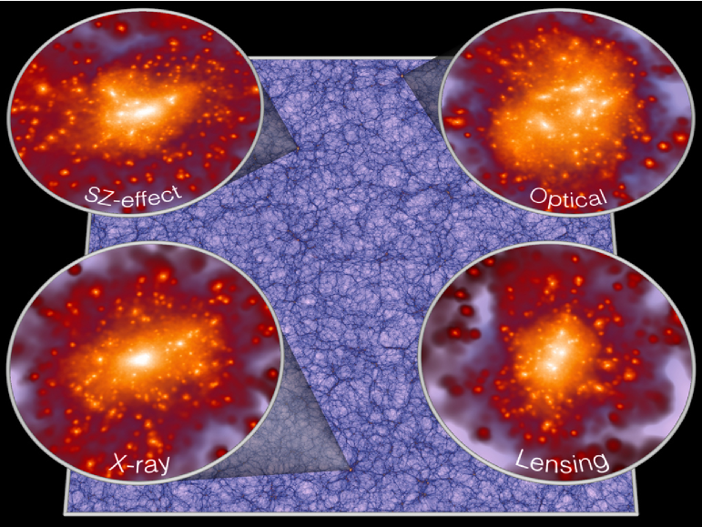
The ‘Millennium-XXL Simulation’ (MXXL) follows the nonlinear growth of dark matter structure within a cubic region of $4.11\,{\rm Gpc}$ ($3\,h^{-1}{\rm Gpc}$) on a side. The dark matter distribution is represented by $6720^{3}=303,464,448,000$ particles, substantially exceeding the number used in all previous simulations of this type (Springel et al., 2005; Kim et al., 2009; Teyssier et al., 2009; Prada et al., 2012) apart from the recent ‘Horizon Run 3’ of Kim et al. (2011), which has 20% more particles but 40 times poorer mass resolution. We note that the simulated volume of the MXXL is equivalent to that of the whole observable Universe up to redshift $z=0.72$. It is more than $200$ times that of our ‘Millennium Simulation’ (MS, Springel et al., 2005), almost 30 times that of the recently completed MultiDark simulation (Prada et al., 2012) but still only 2% that of the Horizon Run 3. The MXXL is also about $7$ times larger than the expected volume of the Baryon Oscillation Spectroscopic Survey (BOSS) (Schlegel et al., 2007) and about twice that of the planed JPAS. Its particle mass is $m_{p}=8.456\times 10^{9}\,{\rm M}_{\odot}$, approximately $7$ times that of the MS but more than $300$ times smaller than that of the ‘Hubble Volume Simulation’ (Evrard et al., 2002), completed a decade ago with a comparable volume to MXXL. The mass resolution of MXXL is sufficient to identify the dark matter haloes hosting central galaxies with stellar mass exceeding $\sim 1.5\times 10^{10}\,{\rm M}_{\odot}$ (De Lucia et al., 2006), and also to predict robustly the internal properties of the haloes corresponding to very massive clusters, which are represented by more than $100,000$ dark matter particles. The Plummer-equivalent softening length of the gravitational force is $\epsilon=13.7\,{\rm kpc}$, which translates into a dynamic range of $300,000$ per dimension, or formally to more than $2\times 10^{16}$ resolution elements within the full simulation volume. This large dynamic range can be appreciated in Fig. 1, where we show the large-scale density field together with the internal structure of a few selected massive clusters.

The MXXL adopts a $\Lambda$CDM cosmology with the same cosmological parameters and output times as the previous two Millennium simulations (Springel et al., 2005; Boylan-Kolchin et al., 2009). This facilitates the joint use of all these simulations in building models for the galaxy population. Specifically, the total matter density, in units of the critical density, is $\Omega_{\rm m}=\Omega_{\rm dm}+\Omega_{\rm b}=0.25$, where $\Omega_{\rm b}=0.045$ refers to baryons (although these are not explicitly treated in the simulation); a cosmological constant, $\Omega_{\Lambda}=0.75$, gives a flat space geometry; the rms linear density fluctuation in $10.96\,{\rm Mpc}$ spheres, extrapolated to the present epoch, is $\sigma_{8}=0.9$; and the present-day Hubble constant is $H_{0}=73\,{\rm km\,s^{-1}Mpc^{-1}}$. Although this set of parameters is discrepant at about the $3\sigma$ level with the latest constraints from CMB and LSS observations (Komatsu et al., 2011), the scaling technique proposed by Angulo & White (2010) (see also Ruiz et al., 2011) allows the Millennium simulations to provide theoretical models for the formation, evolution and clustering of galaxies over the full range of cosmologies allowed by current observational constraints. The parameter offset with respect to the best current observational estimates lies mainly in the high value for $\sigma_{8}$, but this is an advantage for reliable scaling of the simulation results to other cosmologies, as this requires interpolation on the stored MXXL/MS/MS-II data which is only possible for target cosmologies with lower $\sigma_{8}$ than used in the MS.

Figure 1: The projected density of dark matter in the MXXL simulation at $z=0.25$. The insets correspond to circles of radius $5.5\,{\rm Mpc}$ centred on the most extreme clusters identified according to our surrogates for X-ray luminosity, optical richness, lensing signal and integrated thermal tSZ strength (see section 2.3). The underlying image is a projection of the dark matter density in a slab of thickness $27\,{\rm Mpc}$, and width $2050\,{\rm Mpc}$. It is oriented so that it contains three of the selected clusters, as indicated in the figure (the lensing example is from a different slice). The whole simulation box is actually twice as wide, spanning $4110\,{\rm Mpc}$. All four cluster images and the large-scale slice use the same colour scale, which varies in shade from light blue in the least dense regions to orange and white in the densest regions.

2.1.1 Initial conditions

The initial unperturbed particle load for the simulation was built by periodically replicating a $280^{3}$ particle cubic glass file twenty-four times in each coordinate direction. The glass file was created for the MXXL using the method of White (1996) (see also Baugh et al., 1995). The initial conditions were then produced by computing displacements and velocities for each of the particles at starting redshift $z_{\rm start}=63$, using an upgraded version of the code originally developed for the Aquarius Project (Springel et al., 2008). Further improvements include communication and memory optimisations, as well as the use of second-order Lagrangian perturbation theory (2LPT, Scoccimarro, 1998), rather than the Zel’dovich approximation for computing the position and velocity perturbations of each particle. The latter modification is particularly important for the present study, since the abundance of high mass haloes is sensitive to initial transients, which are much smaller and decay more quickly when 2LPT is used (Crocce et al., 2006).

Another important change is the introduction of a new approach to generate Gaussian initial fluctuations. Rather than setting the phases of the modes in $k$-space (as done, for example, in the MS), we first generated a real-space white noise field. The Fourier transform of this field was then used to set the amplitudes of all of the modes needed to make the initial conditions (Salmon, 1996; Bertschinger, 2001; Hahn & Abel, 2011). For the MXXL, the real-space white noise field was created on a $9216^{3}$ grid. Only modes within a spherical $k$-space volume of radius $6720/2=3360$ times the fundamental frequency (i.e. below the particle Nyquist frequency) were used to generate the displacement and velocity fields (all other modes were given zero amplitude).

The use of a white noise field in real space, while not necessary for the MXXL initial conditions themselves, will make it much easier to resimulate arbitrary MXXL regions of interest at higher resolution, for example, the extreme objects illustrated in the present paper. This is because in our new approach it is unnecessary to reproduce the entire white noise field at the original resolution in order to capture the phases of large-scale modes. A consequence is the ability to create consistent sets of initial conditions for resimulations (including ‘resimulations of resimulations’ at yet higher resolution) for arbitrarily defined subregions over a huge dynamic range. The real-space white noise field is generated in a special top-down hierarchical fashion, based on an oct-tree, making it easy to generate coarse representations of the MXXL field at low computational cost. The MXXL white noise field itself occupies just a small subvolume of a single realisation of a huge white noise field created in a hierarchical way. This realisation is specified everywhere to a resolution below the likely free streaming scale of cold dark matter. This means that resimulations of parts of the MXXL volume can be created at any desired resolution as the phases are fully specified everywhere in advance. A full description of this method will be given in Jenkins (2012, in preparation).

2.1.2 The simulation code

Evolving the distribution of the dark matter particles in the MXXL under their mutual gravitational influence was a formidable computational problem. Storing the positions and velocities of the particles in single precision already requires about $7\,{\rm TB}$ of memory. As each particle exerts a force on every other particle, a CPU- and memory-efficient approximate calculation of the forces is of paramount importance. It is also necessary to develop new strategies to deal with the huge data volume produced by the simulation. Using the same analysis approach as for the Millennium Simulation would have resulted in more than $700\,{\rm TB}$ of data, adding a severe data analysis problem and significant disk space costs to the computational challenge.

In order to alleviate these problems, we developed a special “lean” version of the Tree-PM code GADGET-3, which improves the scalability and memory efficiency of the code considerably, outperforming the highly optimised version of GADGET-2 (Springel, 2005) used for the MS. GADGET-3 computes gravitational forces with a TreePM method by combining a particle-mesh (PM) scheme with a hierarchical tree-method, and it uses spatially and temporally adaptive time-stepping, so that short time-steps are used only when particles enter localised dense regions where dynamical times are short. A significant improvement in the new code is a domain decomposition that produces almost ideal scaling on massively parallel computers. Finally, the MXXL version of GADGET-3 uses aggressive strategies to minimise memory consumption without compromising integration accuracy and computational speed. To be specific: (i) We have taken advantage of the unused bits in the 64-bit particle IDs to store various quantities during the calculation, e.g. 4/8-bit floats containing the number of interactions and the acceleration in the previous timestep (these allow us to improve the work-load balance), the group/subhalo membership, and the time-step bin. (ii) Each MPI task contains multiple disjoint sequences of the Peano-Hilbert curve describing the computational domain, resulting in an almost perfect load decomposition. (iii) We avoid storing the geometric center for each node in the tree structure used to compute gravitational forces, reducing the memory requirement at the cost of a slightly less effective tree opening criterion. We also note that we have searched for the combination of force and time-integration parameters that minimises the total execution time for a given desired accurcy in the simulation results.

The code also carries out a significant part of the required post-processing on-the-fly as an integral part of the simulation. This includes group-finding via the Friends-of-Friends (Davis et al., 1985) (FOF) algorithm, application of the SUBFIND algorithm (Springel et al., 2001) to find gravitationally bound subhaloes within these groups, and calculation of basic properties of these (sub)haloes, like maximum circular velocities, cumulative density profiles, halo shapes and orientations, velocity dispersions, etc. These extended halo and subhalo catalogues are then stored at the same output times as for the other Millennium simulations, allowing the construction of detailed (sub)halo merger trees. Full particle data are, however, stored only at a handful of redshifts, very significantly reducing the stored data volume. Only 72 bytes per particle are needed by the simulation code during normal dynamical evolution. When the in-lined group and substructure finders are enabled as well (which is optional), the peak memory consumption per particle increases by a further 26 bytes.

2.1.3 Computational cost and code performance

The MXXL simulation was carried out in the late summer of 2010 on the JuRoPa machine at the Jülich Supercomputing Centre (JSC) in Germany. A partition of 1536 compute nodes was used, each equipped with two quad-core Intel X5570 processors and 24 GB of RAM. We ran our code in a hybrid MPI/shared memory setup on $12,288$ cores, placing one MPI task per processor socket (3072 in total), and employing all four cores of each socket via threads. This setup turned out to be advantageous compared with a pure MPI-parallelisation based on 12888 MPI tasks, because it reduces the amount of intra-node MPI communication, and minimises the RAM required for MPI communication buffers. Also, this makes it easier for our code to reach close-to-optimum work- and load-balance during the calculation.

The final production run carried out approximately 87 trillion force calculations to reach $z=0$, and used about $28.5\,{\rm TB}$ of RAM, nearly the whole available physical memory of JuRoPa. The run-time was $9.3$ days (wall-clock), equivalent to $2.86$ million CPU hours (or $326$ years) in serial. Of this time, 15% were required for running our on-the-fly postprocessing software, notably the group finding, the substructure finding, and the power spectrum calculation, and another 14% were needed for I/O operations. The total long-term storage space required for all MXXL data products is about $100\,{\rm TB}$, down by a factor of about 8 per particle relative to the approach used for the MS and MS-II simulations.

2.2 Basic validation results

Figure 2: The differential Friends-of-Friends (FOF) halo mass function (top panel) of the MXXL (blue), MS (red) and MS-II (green). The MXXL provides vastly superior sampling of the massive end, where the abundance of objects drops exponentially as a function of mass. Combined, the three simulations cover about 8 decades in halo mass. The vertical lines mark the halo resolution limits (20 particles) of the three simulations. For comparison, we also display a fit to the mass function of all self-bound subhaloes in the three Millennium simulations (dashed). The bottom panel gives the ratio of the three mass functions to an analytic fitting formula given in the text. We see that the simulations agree accurately with each other for intermediate masses, but also that different methods for identifying structures disagree significantly in the expected number density of objects of given mass, especially at the high-mass end.

Figure 3: Projected dark matter density for the 15 most massive MXXL haloes (according to $M_{200}$ at $z=0.25$. Each image corresponds to a region of dimensions $6\times 3.7\,h^{-1}$Mpc wide and $20\,h^{-1}$Mpc deep. Note the large variation in shape and internal structure among these clusters. In particular, the most massive cluster, shown in the top left corner, has no clear centre but rather displays several distinct density peaks of similar amplitude.

Figure 4: Matter power spectra measured directly in the MXXL, MS, and MS-II (top panel). The black line shows the power spectrum used to generate the initial conditions, linearly evolved to $z=0$. The dashed lines show the Poisson power level of each simulation, which becomes significant only at the smallest scales. The Poisson power has been subtracted from the measured power spectra in this figure. In the bottom panel, we show the ratio of the measured power spectra to the actual realisation of the linear theory used to generate the initial conditions of each simulation. This procedure reduces sampling noise due to the finite number of modes at small wavenumber. The arrows mark the gravitational resolution limits ($2\pi/$softening length) of the three simulations.

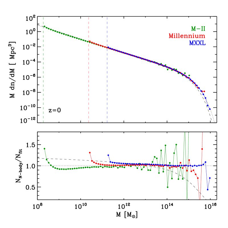
At redshift $z=0$, the MXXL contains more than 700 million haloes with at least $20$ particles. These account for $44\%$ of all the mass in the simulation. Among these objects, $23$ million have a value of $M_{200}$ larger than that of the Milky-Way’s halo ($M_{200}=2\times 10^{12}\,{\rm M}_{\odot}$) and $464$ have a value in excess of that of the Coma galaxy cluster ($M_{200}=2\times 10^{15}\,{\rm M}_{\odot}$). In Fig. 2, we show the differential halo mass function (FoF masses for a linking length $b=0.2$) at the present epoch, which is a robust way of describing the abundance of nonlinear objects as a function of mass (Davis et al., 1985). The most massive halo at $z=0$ has $M_{\rm FoF}=8.98\times 10^{15}\,{\rm M}_{\odot}$. Such extreme objects are so rare that they can only be found in volumes as large as that of the MXXL. We compare the MXXL results with similar measurements from the MS and MS-II simulations. For masses where the three simulations have good statistics and are away from their resolution limits, the agreement is at the few percent level. The results from all three simulations are well described by

$$M\frac{{\rm d}n}{{\rm d}M}=\rho_{0}\frac{{\rm d}\ln\sigma^{-1}}{{\rm d}M}f(\sigma(M)),$$ (1)

where $\rho_{0}$ is the mean mass density of the universe, $\sigma(M)$ is the variance of the linear density field within a top-hat filter containing mass $M$, and $f(\sigma)$ is the fitting function

$$f(\sigma(M))=0.201\times\left[\frac{2.08}{\sigma(M)}+1\right]^{1.7}\,\exp\left[\frac{-1.172}{\sigma^{2}(M)}\right].$$ (2)

The residuals from this analytic halo mass function, displayed in the bottom panel of Fig. 2, show that it describes the numerical results accurately (to better than 5% over most of the mass range) over eight orders of magnitude in halo mass, extending the accuracy of previous models to larger and to smaller scales (e.g. Jenkins et al., 2001; Warren et al., 2006; Tinker et al., 2008). In Fig. 2 the dashed lines show a fit of this same analytic form to the mass function of all self-bound subhaloes (as identified by SUBFIND) in the MXXL, MS and MS-II simulations. These curves correspond to the fit

$$f(\sigma(M))=0.265\times\left[\frac{1.675}{\sigma(M)}+1\right]^{1.9}\,\exp\left[\frac{-1.4}{\sigma^{2}(M)}\right].$$ (3)

The difference between the two fits illustrates how the mass function of objects depends on the way they are defined. This is especially important at the high-mass end. For example, the expected abundance of haloes with $M\sim 10^{15}\,{\rm M}_{\odot}$ changes by a factor of $\sim 2$ when FoF haloes and self-bound subhaloes are compared.

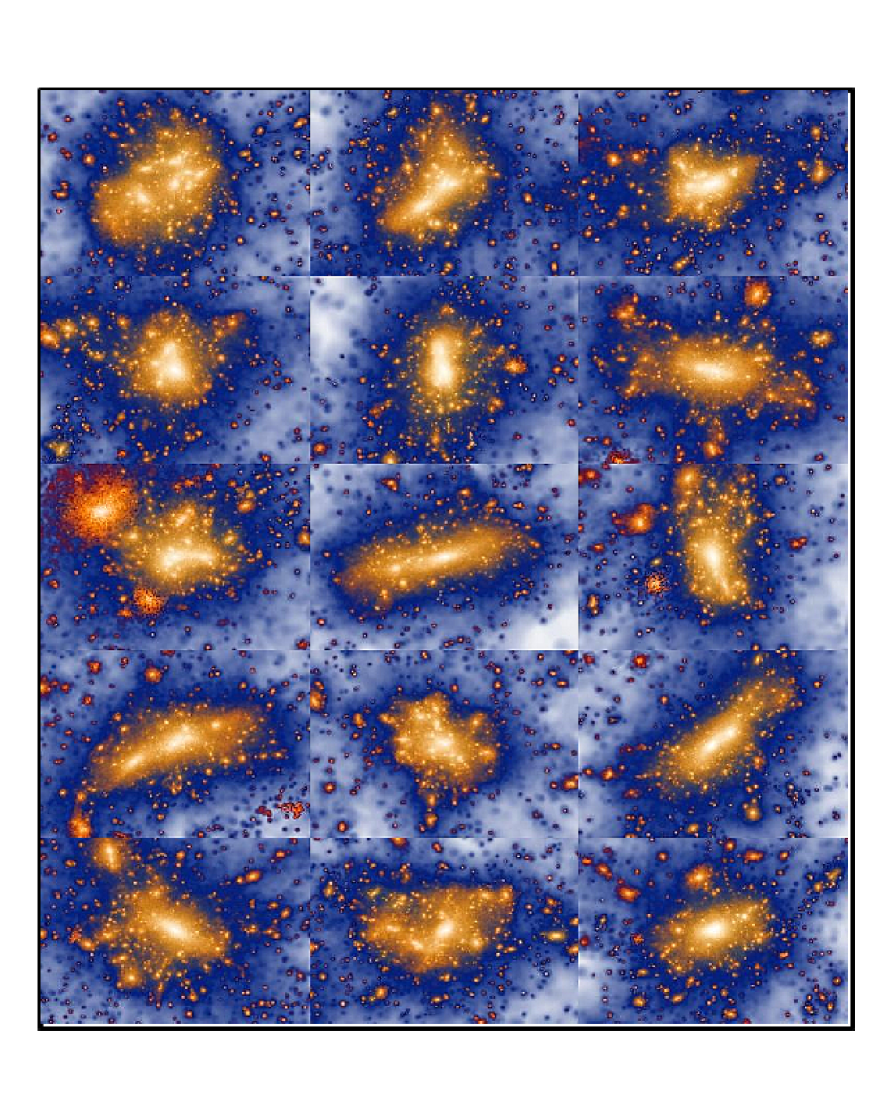
The difficulty in unambiguously defining haloes and their associated mass is in part a consequence of the fact that large haloes do not form a homogeneous population. In fact, they display considerable variety in structure and environment. We illustrate this in Fig. 3 by showing the fifteen most massive clusters in the MXXL at $z=0.25$, selected according to $M_{200}$. Among this group there is considerable diversity in shape, concentration and the amount of substructure, despite all the objects having very similar virial mass. This already suggests that careful modelling of mass estimators will be needed to compare numerical simulations with observed massive clusters at high redshift. Small changes in the estimated mass of an object can dramatically change the predicted probability of its existence within any given cosmological model.

The diversity of massive clusters may also have important consequences for other observational studies. Matched filters are often applied to data in order to maximise the signal-to-noise ratio of, for instance, weak lensing or tSZ detections (e.g. Schneider, 1996; Melin et al., 2006; Rozo et al., 2011). Such filters use a model for the spatial distribution of the signal as prior information (e.g. in the form of density or pressure profiles) but in many cases (and in particular for the most massive objects) the structure of individual clusters will not conform to these assumptions. For instance the top left halo in Fig. 3, which is the most massive cluster in the MXXL at $z=0.25$, does not have a clear centre. In such cases, the signal may be seriously misestimated by a matched filter, potentially biasing cosmological inferences from the measurement.

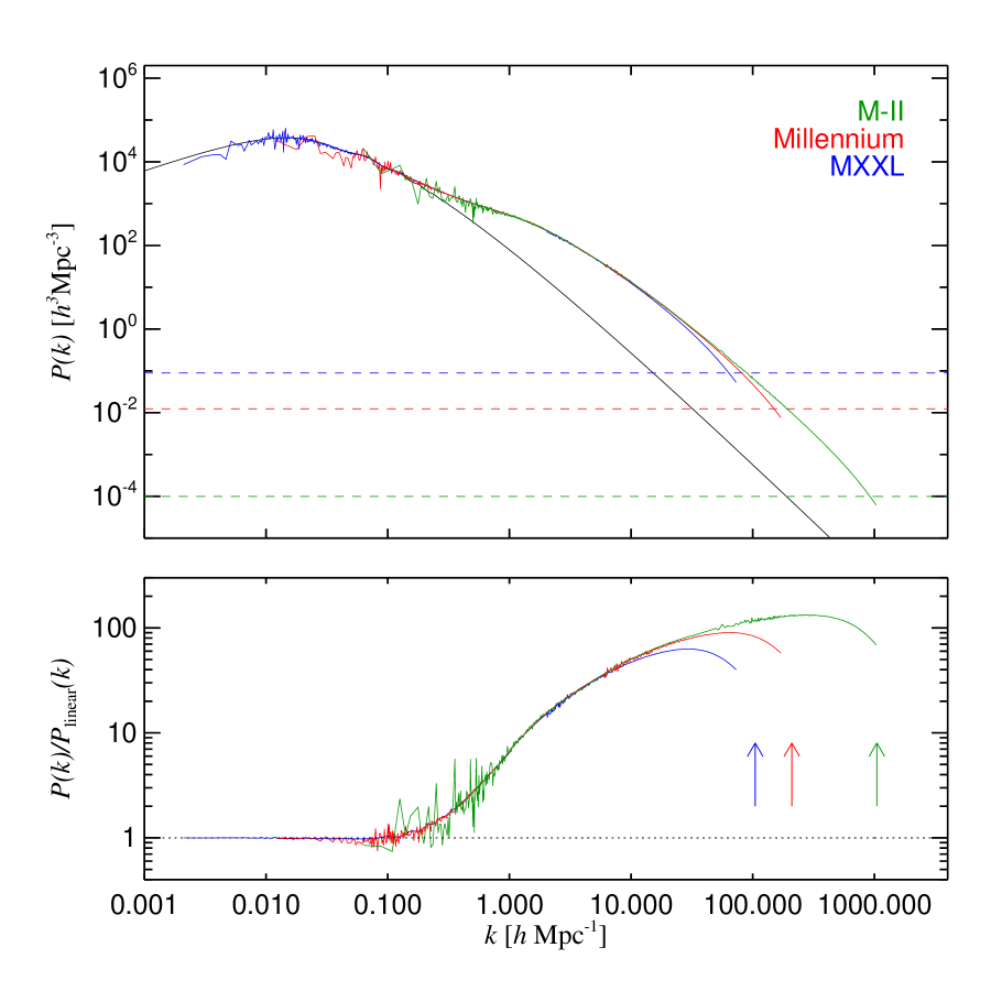
In Fig. 4, we show power spectra of the mass density field at the present epoch. The results are a combination of two measurements. Large-scale modes were computed using a global $9216^{3}$ mesh, whereas the mean amplitude of smaller modes was calculated by folding the density field $64$ times along each direction and projecting it onto a new $9216^{3}$ mesh (Jenkins et al., 1998). This method effectively reaches the same spatial resolution as a $589,824^{3}$ mesh. For comparison, we also show results for the MS and MS-II simulations. Clearly, only the MXXL simulation probes scales significantly beyond the turnover in the power spectrum. The MXXL is also the only one among the three runs that provides good sampling of the baryonic acoustic oscillations (BAO). We note that at low redshift these features already show clear signs of being affected by nonlinear evolution (e.g. Angulo et al., 2008), making the MXXL particularly valuable for studying systematic effects in large-scale galaxy surveys aiming at precise measurements of the BAO features. Throughout the nonlinear regime, the power spectra of the three Millennium simulations show excellent agreement up to the scales where the spatial resolution limits of each run kick in, manifested as a reduction in power relative to higher resolution simulations.

2.3 Surrogate observables

Using the DM distribution and halo catalogues described in the previous section we have created surrogate observables that mimic the four main techniques used observationally to discover and characterise large clusters: optical galaxy counts, gravitational lensing, X-ray emission, and the Sunyaev-Zel’dovich signal imprinted on the microwave background radiation.

Rather than attempting to follow the baryonic physics directly in the simulation, we have constructed simple proxies for these observables, based directly on the dark matter distribution. This necessarily schematic approach avoids the uncertainties of any specific implementation of baryonic processes such as star and black hole formation and the associated feedback, while allowing us to take advantage of the characteristics of the MXXL, namely its combination of very large volume and relatively high mass resolution. Our approach can easily be updated as a better understanding of the relation between the dark matter structure of galaxy clusters and any particular observable is achieved. Our main goal in this paper is not to produce accurate a priori predictions for the observables, but to look for surrogates that correctly rank the expected signal strengths and represent the scatter and the correlations between observables in a realistic way. We can then study the diversity of clusters and quantify the extent to which different methods select different cluster populations.

We focus our analysis on redshift $z=0.25$ because the most massive halo in the observable Universe should be roughly at that redshift (Holz2010). This redshift also corresponds to the median redshift of galaxies in the photometric catalogue of the Sloan Digital Sky Survey (SDSS York et al., 2000), which provides one of the largest samples of optically detected clusters – the MaxBCG catalogue of Koester et al. (2007b), which has been widely used to compute scaling relations for optically selected clusters. Our results do not change qualitatively if we pick another redshift between $z=0$ and $1$. The largest simulated haloes should resemble the most massive observable objects because the MXXL volume is comparable to or exceeds that accessible to real surveys. In $1000$ all-sky light-cones up to $z=0.6$ (built by placing observers randomly on ’Milky Way’ haloes), we find the most massive halo is typically between $z=0.1$ and $z=0.3$, and has a virial mass $M_{200}\sim 4\times 10^{15}\,{\rm M}_{\odot}$, roughly 75% that of the most massive MXXL halo at $z=0.25$, consistent with previous analytic estimates (Holz2010).

Finally, we note that we normalise our surrogates to match observed scaling relations between observables and halo mass (which we discuss in Section 4). This allows a direct comparison of population properties to observational data, side-stepping issues of possible offsets due to incorrect cosmological parameters, to the schematic nature of our surrogates, or to observational details such as filter shapes. We now outline how we construct 2D maps from which we can identify clusters and measure our various surrogate observables.

2.3.1 Optical maps

The first observational approach we consider is the detection of rich clusters in optical surveys, which relies on finding large groups of galaxies in a narrow redshift range and at similar projected positions on the sky. In order to mimic this, we start by constructing a three-dimensional galaxy catalogue using a halo occupation distribution (HOD) model (Kauffmann et al., 1997; Benson et al., 2000; Peacock & Smith, 2000) to populate each MXXL halo with galaxies. We assume that every halo with $M_{200}$ above $1.4\times 10^{12}\,{\rm M}_{\odot}$ hosts one central galaxy and a number of satellites drawn from a Poisson distribution with mean equal to the halo mass in units of $5.7\times 10^{12}\,{\rm M}_{\odot}$ raised to the $0.9$ power. This HOD is similar to that derived for red galaxies in the SDSS (Zehavi et al., 2011), but it is tuned to reproduce the observed mass-richness relation for galaxy clusters as measured by Johnston et al. (2007). The central galaxy is placed at the minimum of the gravitational potential of the dominant SUBFIND substructure in the halo, whereas the satellite galaxies are identified with randomly chosen dark matter particles of the FoF group. The latter ensures that the effects of halo ellipticity, alignment and substructure, which are important for reproducing the small-scale correlations of galaxies (Zu et al., 2008; van Daalen et al., 2012) are included in our modelling. The resulting catalogue at $z=0.25$ contains more than $150$ million galaxies (50% of which are satellites).

We note that the basic assumption of this HOD modelling, namely that the galaxy content of a halo is statistically determined exclusively by its mass, is not expected to hold in detail. Models that follow galaxy formation explicitly predict a dependence of the HOD on other properties such as the halo formation time (e.g. Gao et al., 2005; Zhu et al., 2006; Croton et al., 2007). Nevertheless, these effects are weak so we do not expect them to affect our conclusions. Similarly, moderately different HODs (e.g. models tuned to reproduce the Rozo et al. (2009) mass-richness relation) change the average number of galaxies in our clusters but make little difference to the correlation of optical properties with other aspects of the halo.

2.3.2 Lensing maps

The second identification approach we consider is weak gravitational lensing. Although direct mass measurements using this effect are only possible for the most massive individual clusters, lensing can be used to estimate precise mean masses by stacking a large number of clusters selected according to specific criteria (e.g. Mandelbaum et al., 2006; Sheldon et al., 2009). It is easy to see that orientation effects and both correlated and uncorrelated large-scale structure can play an important role in defining the lensing signal of an individual cluster. As a result, large N-body simulations where the full line-of-sight density distribution is properly modelled are needed to calculate accurately the distribution of expected signals.

Our modelling of lensing maps uses the distant observer approximation. We neglect the evolution of clustering along the line-of-sight and assume that all the mass along a line-of-sight from $z=0$ to $z=1.37$ (the side length of the MXXL) contributes equally to the convergence field. Under these assumptions we create “weak lensing mass maps” by projecting the simulated mass density of the $z=0.25$ snapshot along one axis. MXXL particles are mapped onto a $32,768^{2}$ mesh using a nearest grid point (NGP) mass assignment scheme, yielding an effective transverse spatial resolution of $\sim 92\,h^{-1}{\rm kpc}$.

A more realistic approach would vary the weight assigned to mass at different redshifts assuming a specific redshift distribution for the background source galaxies. The highest weight would go to material which is “halfway” to the sources. Our 4.1 Gpc projection length will clearly tend to overestimate projection effects from distant matter. However, it turns out that structures far in front or far behind the clusters produce only a small fraction of the projection effects; most come from their immediate surroundings and from the directional dependence of the projection of their internal structure. Our simple model can be regarded as treating these aspects quite accurately and as giving an overestimate of the (subdominant) effects of distant projections.

2.3.3 X-ray maps

Another important route to detecting and characterising massive clusters is through X-ray emission from their hot intracluster gas. The local X-ray emissivity is proportional to the square of the gas density and (approximately) to the square root of its temperature. This makes X-rays a particularly sensitive tracer of the inner regions of clusters, where densities can be thousands of times higher than in the outskirts. Simulations with high spatial and mass resolution are needed to probe these inner regions adequately.

We estimate a density local to each particle by using kernel-interpolation over its 32 nearest neighbours, a common method in SPH calculations, while we take the local temperature to be proportional to the velocity dispersion of the subhalo in which the particle is located. Particles outside subhaloes are taken to have zero temperature. With these quantities in hand, we compute a $32,768^{2}$ pixel X-ray map by summing up the density times the square root of the temperature for all the particles along a given line of sight. We note that our X-ray surrogate corresponds to the total bolometric luminosity of a cluster rather than to the luminosity in a particular observational band. However, this has little impact on our results because of the low redshift of our sample and the fact that we scale our surrogates to match observations.

This surrogate clearly neglects dynamical effects on cluster luminosity during violent cluster mergers. Recent hydrodynamical simulations (Rasia et al., 2011) suggest that luminosity enhancements during such events can be substantial, particularly for high Mach number ($>2.5$) and for equal progenitor masses. On the other hand, observational data suggest that disturbed, apparently merging clusters tend to have lower than average X-ray luminosities for their mass, whereas symmetric equilibrium clusters often have cold cores and thus higher than average luminosities (Arnaud et al., 2010). Even the sign of merger effects thus seems unclear.

2.3.4 Thermal SZ maps

The final cluster property we consider is their thermal Sunyaev-Zel’dovich (tSZ) signal (Sunyaev & Zeldovich, 1972, 1980). This effect causes a characteristic distortion of the spectral shape of the cosmic microwave background (CMB) as a result of inverse Compton scattering of CMB photons off the electrons in the hot intracluster plasma. The integrated magnitude of the effect is proportional to the total thermal energy content of the hot electrons in the cluster, or, equivalently, to the gas mass times the mean gas temperature. Along any given line-of-sight the effect is proportional to the line integral of the gas pressure.

In our analysis, we again assume the gas to be distributed like the dark matter and to be isothermal within each quasi-equilibrium subhalo, associating a temperature to each simulation particle proportional to the velocity dispersion of its host subhalo. We then create a $32,768^{2}$ pixel tSZ map by projecting the thermal energies of all MXXL particles along one of the box axes.

3 Results

In this section we use our simulated halo catalogues and mock observational maps to examine various systematic effects that can have an impact on the scatter and mean amplitude of cluster scaling relations. We cumulatively include effects due to sample selection, to spurious cluster identification resulting from projection effects, to misidentification of cluster centres, and to contamination by structures along the line-of-sight, examining in each case the impact on relations between mean tSZ and optical richness, and between weak lensing mass and optical richness.

3.1 Cluster catalogues

We first specify how we identify optical clusters in our galaxy map. We have implemented a group finder similar to that employed to build the MaxBCG cluster catalogue from SDSS galaxies (Koester et al., 2007b). We start by measuring $N_{1}$, the number of galaxies within a cylinder of radius $1\,h^{-1}{\rm Mpc}$ and depth $120\,h^{-1}{\rm Mpc}$ centred on every central galaxy in our catalogues (the depth mimics a redshift uncertainty of $\Delta z\sim 0.02$). Then we discard those galaxies whose cylinder overlaps with that of a central galaxy of a more massive cluster. This is equivalent to assuming that the luminosity of the central Brightest Cluster Galaxy (BCG) increases monotonically with mass, and then discarding as potential group centres those BCGs that are close to a brighter galaxy. After this cleaning procedure we use the galaxy counts around the remaining central galaxies to define a new “observed” cylinder radius $\overline{R}(N_{\rm opt})$, equal to the mean virial radius of clusters of the same $N_{1}$ richness. Then, we repeat the counting and cleaning processes until we reach convergence. We keep all clusters down to a count of one galaxy (i.e. just the central BCG). We refer to this count as the optical richness $N_{\rm opt}$ of the cluster.

A serious systematic in optical cluster catalogues may be caused by misidentification of the BCG, and hence of the center of the corresponding dark matter halo (Rozo et al., 2011). This effect is referred to as ‘miscentering’. In fact, 20% to 40% of the MaxBCG groups (depending on the cluster richness) suffer from this effect according to Johnston et al. (2007). In order to mimic this in our analysis, we have carried out our cluster identification procedure after randomly displacing $30\%$ of our candidate cluster centres according to a 2D Gaussian with a mean shift of $0.4\,h^{-1}\rm{Mpc}$. This distribution of offsets is based on Johnston et al. (2007), who applied the MaxBCG algorithm to mock catalogues built from the Hubble simulation (Evrard et al., 2002). The functional form and parameters we use to describe the effect are also consistent with the distribution of projected distances between the position of the dominant subhalo and that of the second most massive subhalo within haloes of MXXL simulation (see also Fig. 2 of Hilbert & White, 2010). We caution that the miscentering fraction and the displacement parameters are uncertain and are sensitive to details of the cluster-finding algorithm. In Planck Collaboration et al. (2011a) the large X-ray cluster compilation of Piffaretti et al. (2011) was matched to the maxBCG catalogue, finding a median offset between X-ray centre and BCG position of about 100 kpc for the 189 clusters in common; $\sim 15\%$ are offset by more than 400 kpc (J-B Melin, private communication). This agrees reasonably with the result of Johnston et al. (2007). We will see below that few of our results are sensitive to miscentering because it generally causes cluster observables to be perturbed parallel to the scaling relations which link them. Since we retain a flag which notes which of our clusters have had their centres displaced, we can construct a cluster sample based on “true” centres simply by ignoring these objects.

Figure 5: Virial masses ($M_{200}$) for a simulated volume-limited sample of optically detected galaxy clusters at $z=0.25$ as a function of our surrogate observables. Darker regions correspond to a larger number density of clusters. Explicitly, $N_{\rm opt}$  corresponds to a maxBCG-like optical richness, $L_{\rm X}$ to projected X-ray luminosity, $Y_{\rm SZ}$ to projected tSZ signal and $M_{\rm lens}$ to weak lensing mass. All these signals are integrated values within the virial radius, calculated as described in the text, using cluster centres that are randomly displaced 30% of the time from the true potential minima. Dot-dashed lines indicate the expected ‘self-similar’ scalings, while blue solid lines indicate the regressions (in log-log space) of halo mass against each surrogate. These have the slopes listed in each panel which differ from the self-similar expectation. Circles show the mean virial mass for a series of narrow logarithmic bins of each surrogate, while dashed red lines indicate the region containing the central 68% of the clusters in each bin. The fractional scatter in halo mass at given surrogate value is given in each panel.

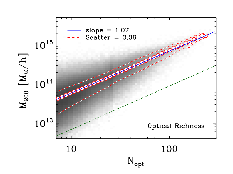
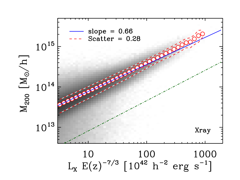
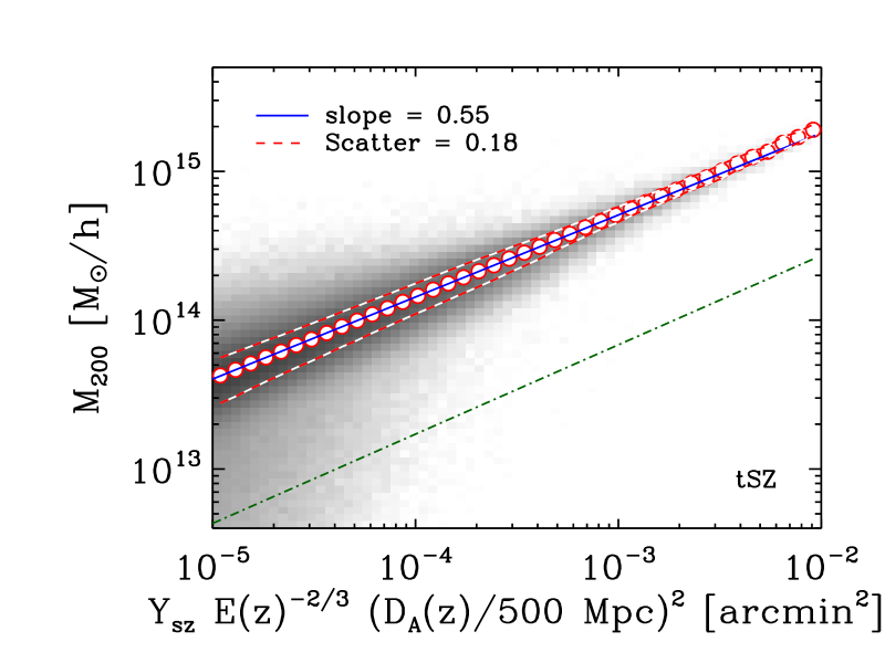
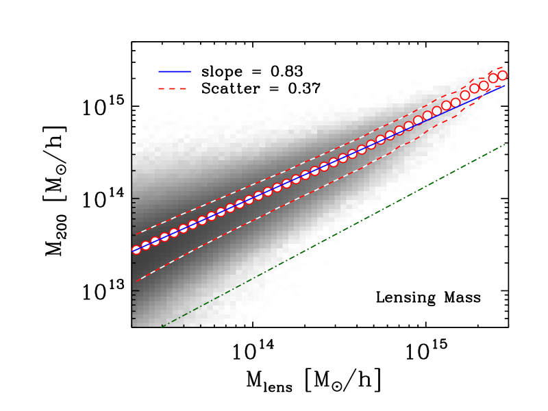
Our catalogue contains $594399$ objects with $N_{\rm opt}$  above $10$, corresponding roughly to haloes with $M_{200}>4\times 10^{13}\,h^{-1}{\rm M}_{\odot}$. There are $1988$ objects with more than 100 members, corresponding to $M_{200}>7\times 10^{14}\,h^{-1}{\rm M}_{\odot}$. For each cluster we compute associated surrogate observables, the X-ray luminosity $L_{\rm X}$, the weak-lensing mass $M_{\rm lens}$, and the tSZ flux $Y_{\rm SZ}$, by integrating the corresponding 2D maps around the apparent (i.e. after ‘miscentering’) centre out to $\overline{R}(N_{opt})$. For each signal we subtract the contribution of the background, which we estimate using an annulus of radius $1.5\times\overline{R}(N_{opt})<r<2\times\overline{R}(N_{opt})$. Naturally, this is not the approach that one would follow for individual well-observed clusters, where one can directly identify the peak of the X-ray, tSZ or weak lensing signals and estimate an individual virial radius from a profile built around this centre. It is, however, closely analogous to the procedure followed when estimating scaling relations (mean values of $M_{\rm lens}$, $L_{\rm X}$ or $Y_{\rm SZ}$ as a function of optical richness) by stacking large samples of optically selected clusters.

In our analysis below, we consider two types of cluster sample that mimic catalogues from large-scale optical and X-ray surveys. By comparing results from these samples we hope to assess the impact of the observational selection method on derived scaling relations (c.f. section 3.2). Koester et al. (2007a) show that, to a good approximation and over a wide range of richness, their maxBCG catalogue can be considered to be selected over a fixed volume of about 0.5 Gpc³. We thus take “optically selected” samples to be selected uniformly from the full MXXL volume, independently of their properties.

Current large “representative” surveys of X-ray clusters are based primarily on the Rosat All Sky Survey (RASS, Voges et al., 1999) and on serendipitous discovery in fields observed for other reasons by the Rosat, Chandra and XMM-Newton satellites. The largest compilations, such as the 1800 cluster MCXC of Piffaretti et al. (2011), are built by combining subcatalogues each of which is effectively X-ray flux limited, and so surveys a substantially larger volume for X-ray bright clusters than for X-ray faint ones. For each subcatalogue, and so for the compilation as a whole, the volume surveyed scales approximately as $L_{\rm X}^{1.5}$ because the apparent luminosity decreases as distance squared whereas the volume increases as distance cubed. This overrepresentation of luminous objects is known as Malmquist bias, and we incorporate it in our “X-ray flux limited” samples by retaining all objects in the MXXL volume but weighting each by the 3/2 power of $L_{\rm X}$.

3.2 Scalings with mass

Figure 6: Correlations among deviations of observables in galaxy clusters with mass in the range $4\times 10^{14}M_{\odot}<M_{200}<1\times 10^{15}M_{\odot}$. Data correspond to logarithmic deviations, i.e. $\Delta\log(s)\equiv\log(s)-\langle\log(s)\rangle$, where the mean is computed for clusters in narrow mass bins ($\Delta\log{M_{200}}=0.2$). The intensity of the background 2D histogram is proportional to the number of haloes in the corresponding region of the plot, with a darker grey-scale indicating a larger number density of objects. Red circles correspond to the average $y$-value in bins along the $x$-axis. The linear correlation coefficient $r$ for each pair of observables is given in the legend of each panel.

Figure 7: Correlations among deviations in $L_{\rm X}$, $Y_{\rm SZ}$ and $M_{\rm lens}$ for objects with optical richness in the range $44<N_{\rm opt}<50$. The intensity of the background 2D histogram is proportional to the number of haloes in the corresponding region of the plot, with a darker grey-scale indicating a larger number density of objects. The linear correlation coefficient $r$ for each pair of observables is given in the legend of each panel.

In Fig. 5 we present the relations between cluster virial mass $M_{200}$ and each of our four surrogate observables for optically detected clusters. Specifically, $N_{\rm opt}$ corresponds to optical richness, $Y_{\rm SZ}$ and $L_{\rm X}$ to the projected tSZ and X-ray fluxes, and $M_{\rm lens}$ to weak lensing mass, all integrated within the projected virial radius corresponding (in the mean) to its estimated richness and surrounding its apparent centre (i.e. after “miscentering” perturbations). The symbols in each panel correspond to the mean of the $M_{200}$ distribution at given value of the surrogate observable and the red dashed lines contain the central 68% of this distribution. The straight blue lines show the linear fit to the individual cluster data (in logarithmic space) which minimises the rms residuals in the vertical direction.

For comparison, green dot-dashed lines indicate the scaling expected naively given our assumptions about the relations between baryonic and dark matter properties. In the optical case, this comes directly from the HOD model used to build the galaxy catalogues ($N_{\rm opt}\propto M^{0.9}$), in the X-ray and tSZ cases from standard self-similar scaling ($L_{\rm X}\propto M^{4/3}$ and $Y_{\rm SZ}\propto M^{5/3}$, respectively), and in the case of lensing it is direct proportionality ($M_{\rm lens}\propto M$). In all four panels, the slope of the measured regression, shown in the legend, is similar but not identical to the expectation. These deviations can be explained by the relative impact for the different surrogates of internal halo structure and of contamination along the line-of-sight, as well as of miscentering. All these can depend systematically on halo mass. The largest discrepancy is found for the lensing surrogate, followed by the optical richness. The smallest are found for the X-ray and tSZ signals. This is consistent with the fact that the stronger the dependence of a surrogate on mass, the less sensitive it is to contamination and to other projection effects, since these are typically produced by less massive systems.

The scatter in halo mass at given value of an observable can be roughly described by a log-normal distribution and depends weakly on the actual value of the observable for those we study here. It is indicated in each panel and ranges from $20$ to $40$%. The tSZ signal shows the least scatter and the lensing the largest. The values we find are consistent with previous studies, but note that our estimators are not optimal (c.f. Melin et al., 2006; Rykoff et al., 2012). Note also that our catalogues do not include all possible sources of scatter, so even larger values may apply to real data. On the other hand, we consider that our results should yield a reliable upper limit on the size of uncorrelated projection effects, given the very large box size of the MXXL. In particular, for tSZ our scatter estimates agree with those reported from full hydrodynamical simulations of smaller volumes (Kay et al., 2012; Battaglia et al., 2011); and for optical richness, with those directly inferred from the data for optical clusters (Rozo et al., 2009). This is a reassuring confirmation that our assumptions are reasonable.

An interesting corollary of the considerable dispersion in these relations is that it is unlikely that the cluster with the largest value for any particular observable will actually correspond to the most massive halo in the survey which identified it. We have explicitly checked that this perhaps counterintuitive situation does indeed hold. In the insets of Fig. 1, we show the most extreme cluster in our simulation as identified by each of our four surrogate observables, i.e. the cluster with the largest tSZ signal, X-ray flux, gravitational lensing signal and optical richness count. These clusters turn out all to be different. The cluster with the largest richness is, in fact, the one with the largest $M_{200}$ at $z=0.25$ and is notable also for the fact that it does not even have a well defined centre. This makes clear that considerable care is needed to draw cosmological inferences from the observed properties of the most extreme cluster in any particular survey. Statistically meaningful constraints can be obtained only with a complete and accurate treatment of the scatter in the mass-observable relation, including any possible dependence on cluster mass.

An important point for our subsequent analysis is that while some sources of scatter affect primarily, or even exclusively, one specific observable, most affect several simultaneously. For instance, at fixed $M_{200}$ the HOD is expected to correlate with halo formation time because older and more relaxed haloes tend to have more dominant BCGs. Since formation time correlates strongly with concentration but only weakly with virial temperature, X-ray luminosity is also expected to increase with halo age, whereas integrated SZ-strength (and also lensing mass) should be age-independent. It has long been clear observationally that at given richness more regular and relaxed clusters (hence “older” clusters) do indeed have more dominant cD galaxies, and it is now clear that they are also more X-ray luminous. In contrast, variations in baryon fraction are expected to affect $L_{\rm X}$ and $Y_{\rm SZ}$ similarly, but to have little effect on $M_{\rm lens}$ and to correlate in a model-dependent and uncertain way with $N_{\rm opt}$. In addition, orientation is expected to have little effect on the measured X-ray luminosity of a cluster but to produce correlated variations in its measured SZ flux, richness and lensing mass. Finally, misidentification of the centre and misestimation of the virial radius of a given cluster will induce variations in all its observables. Generically, such effects imply that deviations from the various mass-observable relations are not independent. Rather, there is a non-zero covariance which reflects common sensitivities to halo structure, orientation, environment and foreground/background superposition – surrogates which are similarly sensitive to these factors are expected to exhibit a high degree of correlation (see also Stanek et al., 2010).

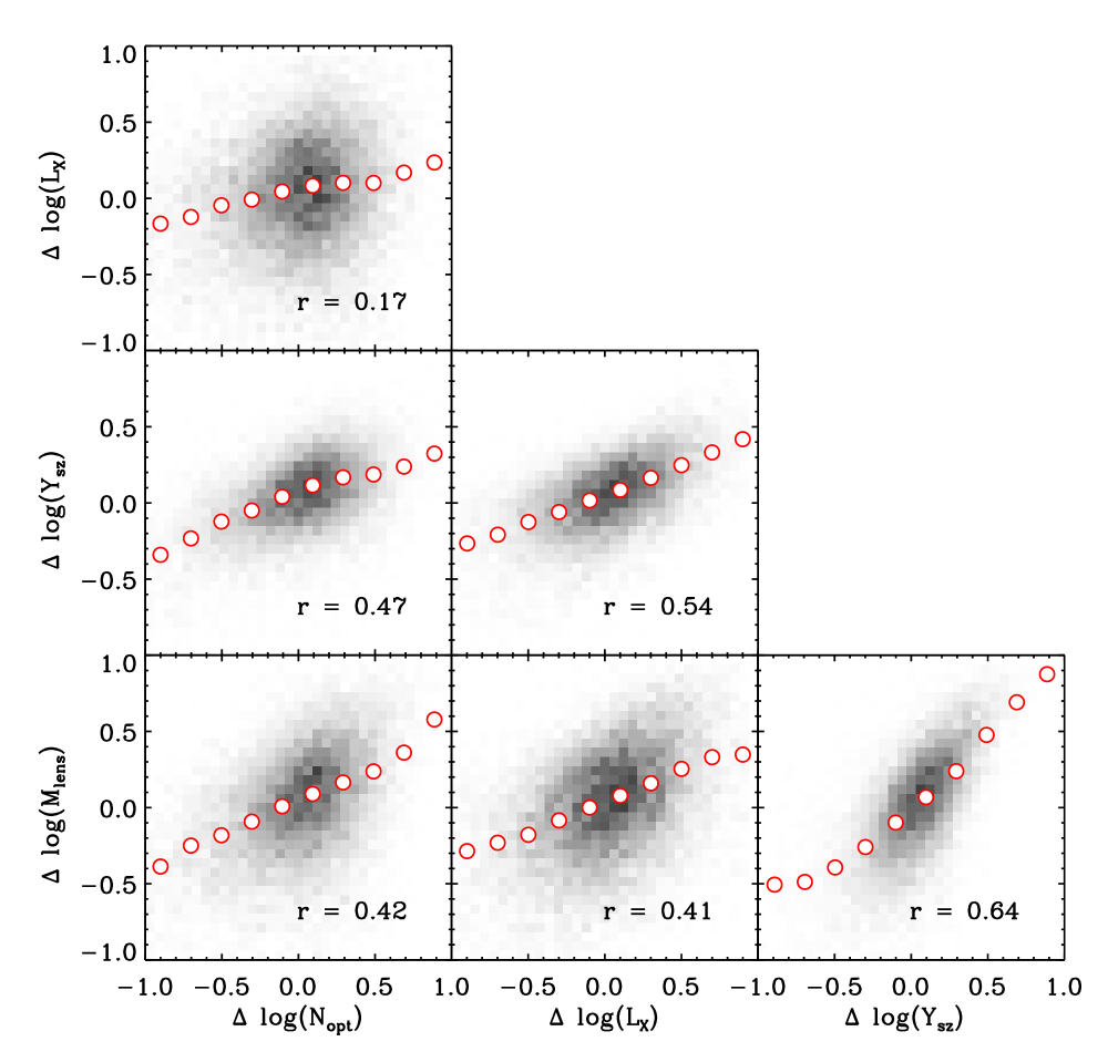
We quantify this effect in Fig. 6 which shows scatter plots of the deviations from the mean at given $M_{200}$ in the logarithms of the values of observables for individual clusters. Here we include all clusters with $1\times 10^{15}M_{\odot}>M_{200}>4\times 10^{14}M_{\odot}$. In each panel we give explicitly the Pearson correlation coefficient, $r$, which characterises the correlation between the deviations.

The strongest correlation is that between the deviations in lensing mass and $Y_{\rm SZ}$, presumably because they are similarly sensitive to cluster orientation, projection, miscentering and misestimation of $R_{200}$. The second strongest is between $L_{\rm X}$ and $Y_{\rm SZ}$, the two quantities sensitive to our estimates of gas density and temperature. The weakest is between richness and $L_{\rm X}$, perhaps because the X-ray luminosity is dominated by the dominant central concentration of clusters while $N_{\rm opt}$ is influenced substantially by orientation and projection effects. The other three correlations are all of similar strength.

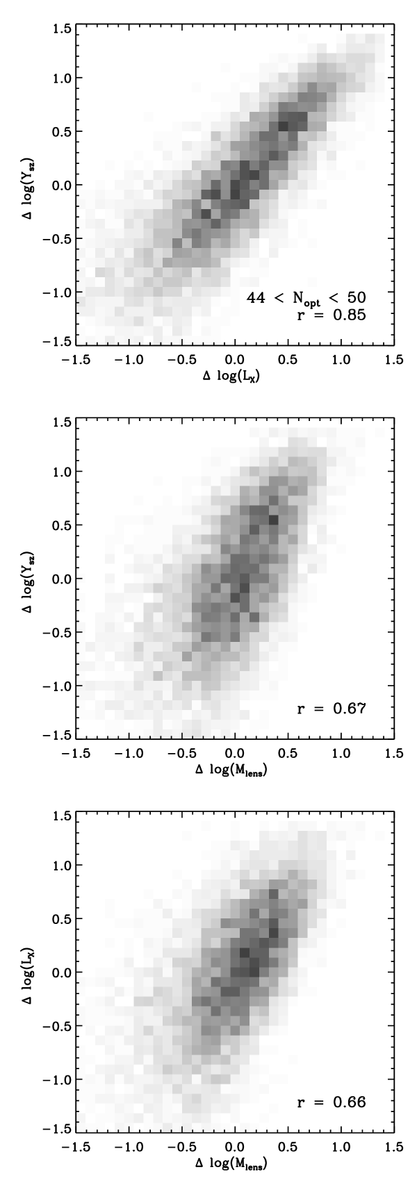
While Fig. 6 illustrates the correlated scatter in observables among clusters of given ’true’ mass, the more relevant correlations for the effects discussed in the next section are those at fixed observed richness, $N_{\rm opt}$. These are shown as scatter plots for $44<N_{\rm opt}<50$ in Fig. 7. We have checked and found quite similar results for other richness ranges. The scatter in each observable is considerably larger at fixed $N_{\rm opt}$ than at fixed $M_{200}$ and the correlations are substantially stronger in Fig. 7 than in Fig. 6, reaching $r=0.85$ for the particularly relevant case of $Y_{\rm SZ}$ versus $L_{\rm X}$.

Despite the different degrees of covariance among our surrogate observables, we note that we measure a positive correlation in all cases. This means that a cluster with an abnormally high signal in one surrogate is likely to have a high signal in the other three as well, especially those where the relevant correlation is strong. Hence, different observables do not provide independent measurements of the true mass of any given cluster, and any analysis which assumes that they do is likely to be at least partially in error. Another implication is that a group of clusters selected using of one of these observables will not form an unbiased sample of the underlying cluster population with respect to any of the other observables. As a result, both the mean scaling relations for such a sample and the scatter around these relations may differ from those for the full underlying cluster population. We will see, for example, that the mass-observable and observable-observable relations derived from an optically selected cluster catalogue will differ in general from those derived from an X-ray selected catalogue.

Figure 8: Thermal SZ signal $Y_{\rm SZ}$ as a function of optical richness $N_{\rm opt}$  for a volume-limited sample of $\sim 500,000$ clusters from the MXXL. The upper panel shows the mean relation and the lower panel the ratio of the scatter to the mean. In each panel the red curve shows the “intrinsic relation” where both the tSZ signal and richness are computed in 3D within a sphere of radius $R_{200}$ centred on the potential minimum. For the “observed” lines, both $Y_{\rm SZ}$ and $N_{\rm opt}$  are computed in projection about these true centres using the true $R_{200}$ and using only uncontaminated clusters, defined to be those where at least 90% of the galaxies are members of a single FoF halo. The “+contaminated” lines refer to samples where this latter condition is eliminated and where the virial radius for each object is estimated iteratively from $N_{\rm opt}$  as is done for real data. Finally, the “+miscentred” curves refer to samples where the projected position of the centre has been offset for 30% of the clusters as described in the text.

3.3 Systematic effects in measured scaling relations

Figure 9: SZ signal $Y_{\rm SZ}$ as a function of optical richness $N_{\rm opt}$  for a X-ray flux limited sample of $\sim 500,000$ clusters from the MXXL. This is directly analogous to Fig. 8 and was constructed in the same way except each cluster is weighted by the 3/2 power of its X-ray luminosity. The “observed”, “+contaminated” and “+miscentered” lines refer to the same cluster sets as in Fig. 8, differing only because of this weighting. The red lines labelled “volume limited” repeat the “+miscentered” results from Fig. 8. Malmquist effects substantially enhance the amplitude of the mean relation, reduce the scatter, and make the relation insensitive to superposition and miscentering effects.

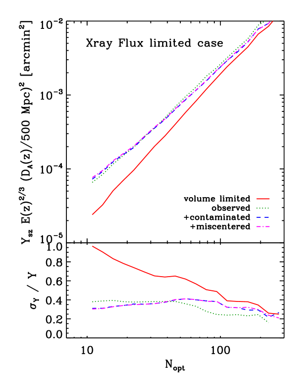
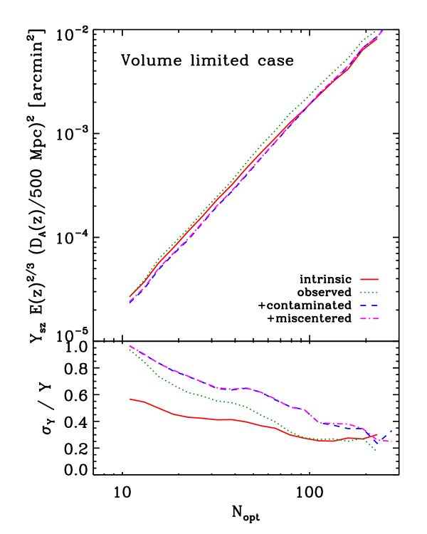
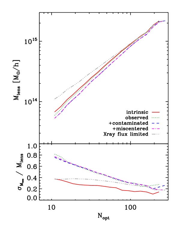
We now consider how the thermal SZ signal is related to optical richness for cluster samples selected in various ways. In Fig. 8 we display results where each MXXL cluster is assigned equal weight in order to mimic volume-limited samples like the optically selected maxBCG survey. For comparison, in Fig. 9 we show results where each cluster is weighted by $L_{\rm X}^{3/2}$, mimicking cluster samples like the MCXC which is constructed from a number of X-ray surveys, each of which is effectively X-ray flux limited. The upper panels in these plots show mean $Y_{\rm SZ}$ for clusters of given $N_{\rm opt}$, while the lower panels show the rms scatter about these relations expressed as a fraction of the mean signal. Lines in the upper panels thus represent the mean tSZ signals expected if clusters from optical or X-ray surveys are stacked as a function of their optical richness.

The solid red lines in Fig. 8 show the “intrinsic” relation which is obtained if both $Y_{\rm SZ}$  and $N_{\rm opt}$  are calculated in 3D by integrating over a sphere centred on the potential minimum and with radius $R_{200}$. The properties of real clusters are, of course, measured from 2D maps. The dotted lines labelled “observed” in both figures show the relations obtained for uncontaminated clusters when both $Y_{\rm SZ}$ and $N_{\rm opt}$ are integrated over a disk around the potential minimum with radius given by the true $R_{200}$. Here “uncontaminated” means that at least 90% of the galaxies contributing to $N_{\rm opt}$ have to lie in a single FoF halo. Although, by definition, our estimates of $N_{\rm opt}$ and $Y_{\rm SZ}$ both increase for any individual object in going from 3D to 2D, they increase by similar amounts, with the result that the apparent relation does not change significantly over the full range of richness probed here. The scatter, on the other hand, is greatly increased for poor clusters, where it can double the intrinsic value, but is little affected for rich clusters.

For the dashed blue lines labelled “+contaminated” in Figs. 8 and 9 we relax the requirement that the clusters be uncontaminated. We also use an observational estimate of $R_{200}$ for each cluster when estimating its richness and its tSZ signal, as described earlier in this section. Line-of-sight superposition effects then contribute to the values of all the observables. Because the superposed objects are usually of lower mass (and hence lower temperature) than the main cluster, they typically inflate $N_{\rm opt}$ (which scales approximately as $M^{0.9}$) more than they do $Y_{\rm SZ}$ (which scales approximately as $M^{5/3}$). As a result, the “+contaminated” relations lie slightly to the right of the “uncontaminated” ones. The effect is smaller in Fig. 9 than in Fig. 8. The scatter is further increased by contamination in the volume-limited case but is relatively little affected for flux-limited samples.

The final observational systematic we study is miscentering. The dot-dashed purple curves labelled “+miscentering” in Figs. 8 and 9 show the relations found when the centres assigned to a random 30% of the clusters are offset from their potential minima as described above. This results in a surprisingly small shift in the mean relation in both cases. Again, this is because such offsets induce shifts in the estimated values of $N_{\rm opt}$ and $Y_{\rm SZ}$ that are largely parallel to the mean relation.

These “+miscentering” curves give our most realistic estimate of the relations expected for real clusters in the two cases. We repeat these (dot-dashed purple) curves from Fig. 8 as solid red curves in Fig. 9 in order to emphasise the most important result of this section. The average $Y_{\rm SZ}$ signal for X-ray flux-limited samples is boosted by a factor of $3.5$ in the low richness tail and by a factor of $1.25$ at high richness, relative to the volume-limited case. This is a consequence of the strong correlation between $L_{\rm X}$ and $Y_{\rm SZ}$ at fixed $N_{\rm opt}$ which is visible in the top panel of Fig. 7. In samples selected above a limiting X-ray flux, clusters of given $N_{\rm opt}$ which are X-ray underluminous are down-weighted and these tend also to be the objects with the smallest $Y_{\rm SZ}$ signals. This is a manifestation of Malmquist bias.

Figure 10: Mean lensing mass as a function of optical richness for clusters in the MXXL simulation. “Lensing mass” is defined as the mass within a properly centred sphere of radius $R_{200}$ ($M_{200}$, the red solid curve labelled “intrinsic”) or projected within a circle of radius given by an $N_{\rm opt}$-based estimate of $R_{200}$ and centred either on the true potential minimum (“observed” and “+contaminated” cases) or on an offset centre in 30% of the cases (“+miscentred”). $N_{\rm opt}$  is defined within these same regions. The upper panel shows the mean relations while the lower one gives the fractional scatter about these relations. The “X-ray flux limited” curves refer to the “+miscentred” case with haloes weighted by $L_{\rm X}^{3/2}$.

A second important consequence of X-ray selection is that the scatter about the mean $Y_{\rm SZ}$-$N_{\rm opt}$ relation is greatly reduced. The lower panel of Fig. 9 shows that we predict it to be only about half that for a complete volume-limited sample of clusters. Although much of this difference is due to a reduced sensitivity to contamination and miscentering, the scatter is lower even than that shown in Fig. 8 for uncontaminated and properly centred clusters. If not corrected, this could lead to over-optimistic estimates of the performance of mass estimators when tested on X-ray selected cluster samples. Such samples are clearly more homogeneous in internal structure at given mass than volume-limited samples. We expect biases of this kind to be present in any cluster catalogue selected according to a specific observable, and they must be corrected in order to infer correctly, for example, the volume abundance of clusters as a function of $M_{200}$, the quantity normally used to draw cosmological conclusions from the cluster population. Robust constraints require not only that the mean transformation from observable to mass be determined accurately and without bias, but also that the scatter between these quantities be known to high precision.

Fig. 10 is analogous to the previous two figures but now focuses on the relation between gravitational lensing mass and richness. As was the case for $Y_{\rm SZ}$-$N_{\rm opt}$, we find that the slopes of the mean relations are similar in all the volume limited cases, and that the effects of contamination and miscentering are quite modest. In contrast to Johnston et al. (2007), who find that miscentering decreases the normalisation of the $M_{\rm lens}$-$N_{\rm opt}$ relation by 15-40% (see their Tables 3 and 8), it barely changes the mean relation in our data. This is because of the strong correlation between our estimators of optical richness and lensing mass. If the center of a halo is misidentified, both $N_{\rm opt}$ and $M_{\rm lens}$ are underestimated, and the change is, on average, almost parallel to the mean relation. The stronger effect seen by Johnston et al. (2007) may reflect their different estimator for the lensing mass, or possibly a failure to account consistently for the implied change in richness. We note that this richness reduction implies that at any given $N_{\rm opt}$, fewer than 30% of clusters will actually be miscentered, both because cluster abundances increase steeply with decreasing richness, and because poor clusters are more likely to be rejected by our algorithm in favour of richer overlapping systems. Note also that the mean lensing mass is biased high by the Malmquist effect in X-ray flux limited cluster samples because at given richness more luminous clusters are usually more massive.

The various biases examined here depend both on the intrinsic properties of the cluster population and on the specific technique used to measure each observable. For instance, the smaller the scatter between X-ray luminosity and optical richness, the smaller the impact of Malmquist bias on the amplitude of the $Y_{\rm SZ}$-$N_{\rm opt}$ relation. In the limiting case of no scatter the relations for flux-limited and volume-limited samples would be identical. The same would be true if there were no correlation between $L_{\rm X}$ and $Y_{\rm SZ}$ at fixed $N_{\rm opt}$. The substantial effects found above are due to the strong correlations we predict. The details of the observational procedures matter because they can enhance or suppress the impact of different aspects of the data. For instance, an optimal filter based on expected cluster profiles will be more sensitive to miscentering than a top-hat filter of large size; the shear profile scheme which Johnston et al. (2007) used to estimate lensing masses may be yet differently sensitive. Such effects must be taken into account properly if any particular survey is to place reliable constraints on cosmological parameters. This also applies to inferences from the properties of extreme objects. Cosmological inferences require a full understanding of the scatter in the observable-mass relation and an accurate knowledge of the selection function, otherwise one may arrive at seriously erroneous conclusions.

4 Scaling relations for Planck clusters

Figure 11: Comparison of scaling relations between observed and simulated clusters. The left-hand panel shows X-ray luminosity as a function of optical richness. The red circles with error bars show the mean luminosity of stacks of MaxBCG clusters as measured by Rykoff et al. (2008a), while blue points indicate individual maxBCG clusters which are also in the MCXC compilation of Piffaretti et al. (2011). The right-hand panel shows the tSZ signal as a function of optical richness. Here, red circles indicate mean values for stacks of the entire maxBCG catalogue, while blue circles are for stacks of maxBCG clusters that are also in the MCXC (Planck Collaboration et al., 2011c). All observational data correspond to the equivalent of measurements within $R_{500}$ and at $z=0$. Predictions from the MXXL simulation are shown by red lines for a volume-limited sample and by blue lines for a X-ray flux-limited sample. Note that the normalisations of our $L_{\rm X}$ and $Y_{\rm SZ}$ proxies are set by shifting the red lines vertically to give the best possible fit to the red circles in these two plots.

In the last section, we showed that cluster scaling relations are strongly and systematically affected by the way in which cluster samples are selected. This is a consequence of the substantial scatter in mass-observable and observable-observable relations, and the fact that deviations of different observables from the mean relations are strongly correlated because of common sensitivities to cluster structure, orientation, environment, and line-of-sight projection. The resulting distortion of scaling relations depends on how clusters are detected and their observables measured, so precise correction requires detailed modelling of each individual experiment. Our catalogues based on surrogate observables are nevertheless realistic enough to examine whether effects of this kind might explain some apparent inconsistencies recently highlighted by the Planck Collaboration.

There are three pieces to the puzzle presented by the Planck collaboration. First, the mean tSZ signal for stacks of maxBCG clusters of given optical richness is about half of that predicted by scaling relations derived from the much smaller REXCESS sample for which individual X-ray profiles are available (Böhringer et al., 2007). The hot gas structure of the REXCESS sample is well described by the almost self-similar scaling of a “universal” pressure profile which resembles that predicted by hydrodynamical simulations of cluster formation (Arnaud et al., 2010). The REXCESS scaling relations do, however, agree well with the mean $Y_{\rm SZ}$ measured when clusters from the large MCXC compilation (Piffaretti et al., 2011) are stacked as a function of $L_{\rm X}$ (Planck Collaboration et al., 2011b). Note that comparison with the stacked $Y_{\rm SZ}$-$N_{\rm opt}$ relation for maxBCG sample requires an estimate of cluster mass as a function of $N_{\rm opt}$, for which Planck Collaboration et al. (2011c) used weak lensing results for stacked maxBCG clusters (Johnston et al., 2007; Rozo et al., 2009).

The second piece of the puzzle is that if the maxBCG sample is restricted to clusters which are also in the MCXC, the stacked $Y_{\rm SZ}$-$N_{\rm opt}$ relation lies well above (a factor of 2 at ${N_{\rm opt}}=50$) that for the sample as a whole and appears consistent with the REXCESS scaling relations. The third and final piece is that the relation between mean $Y_{\rm SZ}$ and mean $L_{\rm X}$ signals for stacks of the full maxBCG binned by $N_{\rm opt}$ is consistent both with that between mean (stacked) $Y_{\rm SZ}$ and $L_{\rm X}$ in the MCXC and with that between $Y_{\rm SZ}$ and $L_{\rm X}$ for individual clusters in the REXCESS sample. All these facts led the Planck Collaboration to speculate that a subset of optically detected clusters might have very weak tSZ and X-ray signals, presumably because they contain many galaxies but rather little hot gas.

We now examine these issues using suitably selected cluster catalogues from the MXXL. To mimic the full maxBCG catalogue, we use volume-limited samples (c.f. Koester et al., 2007a) and we measure a “maxBCG-like” richness for each as detailed in Section 3.1. To mimic the MCXC, we will use “X-ray flux limited” samples which weight each object by $L_{\rm X}^{3/2}$, since Piffaretti et al. (2011) built the MCXC by combining a number of X-ray surveys, most of which are effectively flux-limited. We are also interested in the overlap between these two observational samples. At high X-ray luminosity clusters are detected in the RASS to distances beyond the limit of the maxBCG catalogue, so that the combined sample is effectively volume-limited. At low X-ray luminosity, on the other hand, the maxBCG limit is well beyond the distance at which RASS can detect clusters and the overlap sample is flux-limited. As we will see below, the effects of this change in sample selection are directly visible in the behaviour of the stacked $Y_{\rm SZ}$ signal of the overlap sample.

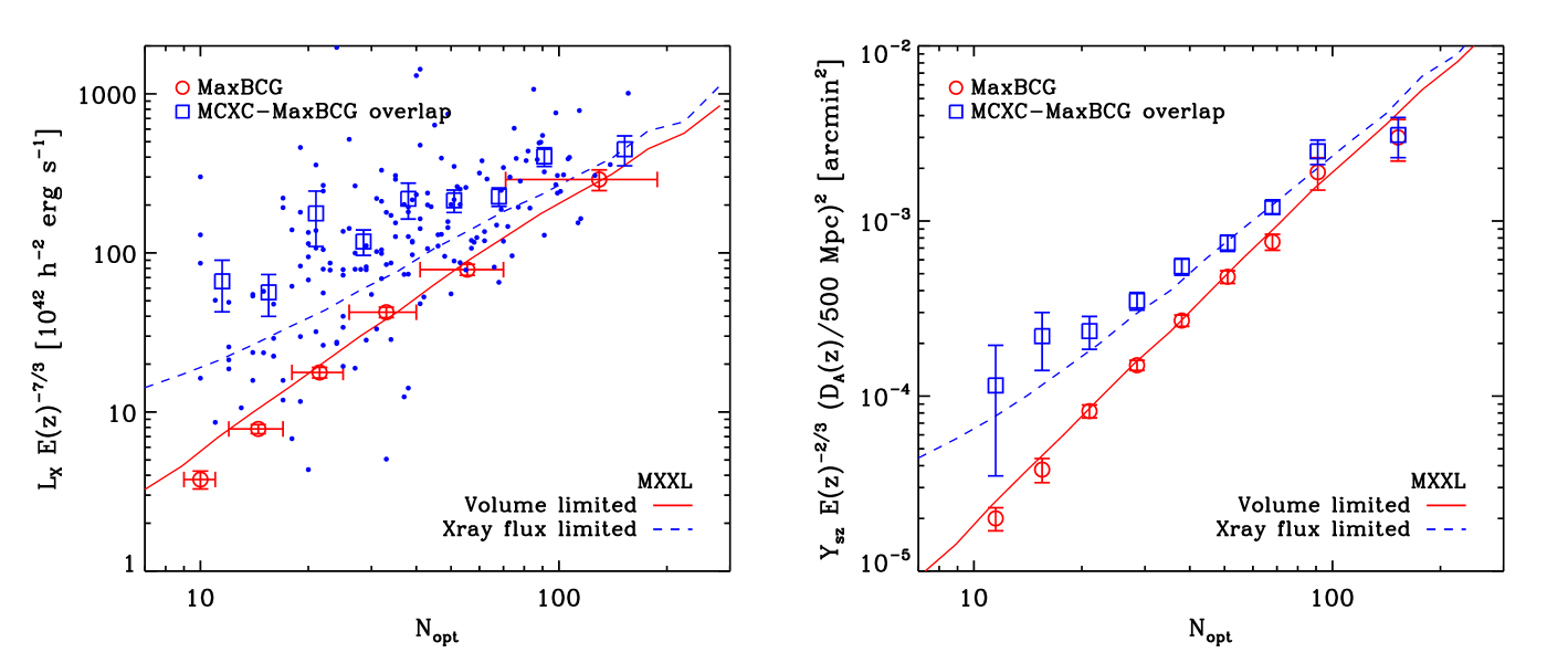
We begin by considering the mean X-ray luminosity and mean tSZ signal as functions of optical richness for MaxBCG clusters. These data are displayed in Fig. 11 as red circles. In the left panel, we show X-ray measurements from Rykoff et al. (2008a) which correspond to the average X-ray luminosity within $R_{500}$ for stacks of RASS maps centered on MaxBCG clusters. We convert their luminosities, originally measured within $R_{200}$, to ones measured within $R_{500}$ by multiplying them by $0.91$. We also scale these values to their $z=0$ equivalent by assuming a self similar scaling of the luminosities. In the right panel we show the average tSZ signal in Planck maps within $R_{500}$ for the same richness-binned MaxBCG clusters. Note that the mass-richness relation from Rozo et al. (2009) was used to set the size of the matched filter when measuring the $Y_{\rm SZ}$ signals, but that this has little impact on the result and is unimportant for our discussion here.

We now compare these results to our simulation. Red lines show the mean relation predicted by “observational” catalogues which include both contamination and miscentering. They have been shifted vertically to fit the maxBCG data as well as possible, thus determining the scaling coefficients used consistently in our $L_{\rm X}$ and $Y_{\rm SZ}$ proxies throughout this paper. After this normalisation, the $Y_{\rm SZ}-N_{200}$ and $L_{\rm X}-N_{200}$ relations are predicted remarkably well. The latter relation in the MXXL is slightly shallower than observed. This reflects the well known fact that the observed $L_{\rm X}$-$T_{\rm X}$ relation is steeper than that expected from the self-similar model on which we built our surrogates, apparently indicating a systematic variation in gas fraction or concentration with cluster mass. The agreement nevertheless appears good enough to validate our approximate modelling of gas physics, suggesting that it is adequate to capture the statistical correlations underlying the influence of selection bias on cluster scaling relations.

The second set of observations in Fig. 11 refer to the set of $189$ maxBCG clusters which are also in the MCXC. Blue dots in the left-hand panel show $L_{\rm X}$ as a function of $N_{\rm opt}$ for the individual clusters, whereas blue squares in the both panels give average values for stacks of these clusters around their maxBCG centres, using the same $N_{\rm opt}$ bins as for the full maxBCG sample (Planck Collaboration et al., 2011c). In both cases we plot the $z=0$ equivalent value, using the measured redshift for each cluster and assuming a self-similar scaling of the signals. This allows a consistent comparison of all datasets.

As noted by the Planck Collaboration, stacked tSZ fluxes are systematically larger for MCXC clusters than for the full MaxBCG sample, except possibly for the richest systems. The left panel ofFig. 11 indicates that their X-ray luminosities are also systematically higher, again with the possible exception of the richest clusters. Blue dashed lines in both panels indicate the mean relations we predict for X-ray flux limited samples. The Malmquist bias offset from the volume-limited relation explains part of the difference between the blue squares and the red circles in the left panel, and it explains almost completely the discrepancy in the right panel. As discussed in the last section, the latter is caused by a strong correlation between the deviations of individual clusters from the mean $L_{\rm X}$-$N_{\rm opt}$ and $Y_{\rm SZ}$-$N_{\rm opt}$ relations. This causes Malmquist bias to propagate from X-ray selection into the $Y_{\rm SZ}$- $N_{\rm opt}$ relation. This suggests that the correlated scatter between $L_{\rm X}$ and $Y_{\rm SZ}$ at given $N_{\rm opt}$ is well represented in our model, but also that there are sources of scatter which only affect $L_{\rm X}$ that are not accounted for in our analysis which would increase the difference between X-ray scaling relations derived from volume and X-ray flux limited samples without affecting the $Y_{\rm SZ}$ signal.

Finally, we reiterate that both relations have considerable scatter. At given $N_{\rm opt}$ our model indicates that the fractional uncertainty in $L_{\rm X}$ and $Y_{\rm SZ}$ for volume-limited samples is about $40\%$ for $N_{\rm opt}$ $\sim 200$ and rises to $130\%$ for $N_{\rm opt}$ $\sim 10$. These numbers are broadly consistent with the intrinsic scatter reported by Planck Collaboration et al. (2011c) for the SZ measurement of MaxBCG clusters. The corresponding fractional scatters are about $40\%$ for both $L_{\rm X}$ and $Y_{\rm SZ}$ in our X-ray flux limited samples.

Figure 12: Average tSZ flux as a function of average X-ray luminosity for clusters stacked according to optical richness. Red solid and blue dashed lines give MXXL results for our volume-limited and X-ray flux limited samples, respectively and refer to the same set of $N_{\rm opt}$ bins. Both $L_{\rm X}$ and $Y_{\rm SZ}$ are larger for the flux-limited sample, but the shift is almost parallel to the mean relation so that Malmquist bias has little visible effect. Red circles are taken from Planck Collaboration et al. (2011c) and refer to maxBCG clusters, whilst blue squares are the results for the subset of clusters present in the MCXC catalogue. In both cases the data are binned according to $N_{\rm opt}$. Error bars indicate bootstrap uncertainties in the mean $L_{\rm X}$ and $Y_{\rm SZ}$ signals in each richness bin. The green dotted line shows the predictions of the X-ray model build by Planck Collaboration et al. (2011c).

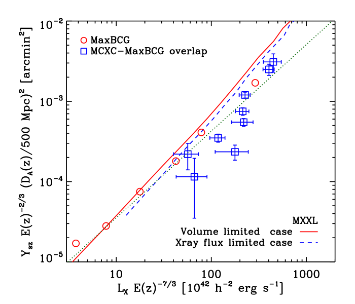
We now move to another observable scaling relation reported by PLANCK: that between $Y_{\rm SZ}$ and $L_{\rm X}$. We display simulation results for both volume-limited and X-ray flux limited catalogues in Fig. 12. Clusters were stacked as a function of $N_{\rm opt}$ and then the mean $Y_{\rm SZ}$ of each stack was plotted against its mean $L_{\rm X}$. Although both $Y_{\rm SZ}$ and $L_{\rm X}$ are substantially larger at given $N_{\rm opt}$ in flux-limited stacks, the two relations are almost identical. Malmquist bias has a negligible impact because the shifts are almost parallel to the mean relation.

The same relation can be constructed for the (almost) volume-limited maxBCG catalogue by stacking RASS and Planck data for clusters binned by $N_{\rm opt}$. This exercise was carried out by Planck Collaboration et al. (2011c) and their result is overplotted in Fig. 12. We also include, as a green dotted line, the relation predicted by the X-ray model built by Planck Collaboration et al. (2011c) based on observations of REXCESS clusters and an observational $N_{\rm opt}$-$M_{\rm lens}$ calibration. Despite the relations being built from different samples, they are very similar to each other and to our MXXL predictions, showing not only that the $Y_{\rm SZ}$-$L_{\rm X}$ relation is insensitive to details of sample definition, but also that our proxies continue to represent the observables well in this plane.

An $Y_{\rm SZ}$-$L_{\rm X}$ relation for the effectively flux-limited MCXC-maxBCG overlap is also shown in Fig. 12. For the richest optical bins, it is compatible with all other relations, but the $L_{\rm X}$ signal is considerably larger for poor clusters. The relatively small number of systems per bin leaves room for this to be a statistical fluctuation (and indeed, we find that the median per bin agrees much better with the expected relation). However, if real, it indicates that the differences in $Y_{\rm SZ}$ and $L_{\rm X}$ at fixed $N_{\rm opt}$ cannot be explained by the existence of a subpopulation devoid of hot gas, as suggested by Planck Collaboration et al. (2011c), since this would move the points in Fig. 12 along a line of slope unity and so could not bring them back onto the relation for the full maxBCG sample. On the other hand, all data can be simultaneously explained by Malmquist bias, together with an extra source of scatter affecting only $L_{\rm X}$ (e.g. the presence or absence of cool cores in the gas distributions). Note that this requires correlated scatter in observables of the kind illustrated in Fig. 6 and Fig. 7 and does not work in simpler treatments of the same puzzle, as that of Biesiadzinski et al. (2012) which does not fully incorporate all such correlations.

Given that our simulation appears to reproduce consistently all the measured observable-observable relations for the maxBCG and MCXC catalogues, it is interesting to discuss why the Planck collaboration’s modelling gave a prediction which was inconsistent with the measured $Y_{\rm SZ}$-$N_{\rm opt}$ relation for the maxBCG sample. The answer appears to lie in the way cluster masses were used to relate the population identified in X-ray surveys to the maxBCG clusters. Since values of $N_{\rm opt}$ are not available for most of the clusters in bright and well studied X-ray samples, this richness measure must be calibrated against another observable if the hot gas properties of such samples are to be used to predict the mean $Y_{\rm SZ}$ signal from maxBCG stacks. X-ray luminosity could have been used, since Rykoff et al. (2008b) provide mean $L_{\rm X}$ values as a function of $N_{\rm opt}$, and the $Y_{\rm SZ}$-$L_{\rm X}$ relation is not only theoretically robust but also observationally well determined (see Fig. 12). This route ($N_{\rm opt}\rightarrow{L_{\rm X}}\rightarrow{Y_{\rm SZ}}$) predicts mean $Y_{\rm SZ}$ values for maxBCG stacks which agree well with those measured directly. However, the Planck collaboration decided instead to follow a different route ($N_{\rm opt}\rightarrow M_{500}\rightarrow{Y_{\rm SZ}}$) using the mean weak lensing masses measured as a function of $N_{\rm opt}$ for stacked maxBCG clusters by Johnston et al. (2007) and Rozo et al. (2009) who in addition corrected $M_{\rm lens}$ upwards to account for an improved model for the redshift distribution of the source galaxy population. Both these studies made substantial upward corrections to the directly measured mean masses to account for the effects of line-of-sight contamination and miscentering, but they failed to make consistent corrections to $N_{\rm opt}$, thus ignoring the correlated deviations of individual clusters from the mean $N_{\rm opt}$-$M_{200}$ and $M_{\rm lens}$-$M_{200}$ relations which are visible in the lower left panel of Fig.6. Thus, the reported scaling relations correspond to the relationship between the true mass of a cluster and its miscenterd optical richness, and so predict the $Y_{\rm SZ}$ signal expected for well-centered clusters as a function of their miscentered richness. These predictions should not be compared against Planck data, unless the $Y_{\rm SZ}$ is corrected for miscentering in a similar way to the weak lensing data.

An alternative is to use the uncorrected measurements, because the correlation among observables results in an apparent $N_{\rm opt}$-$M_{\rm lens}$ relation almost identical to that of well-centered and uncontaminated clusters. In fact, if the original “raw” masses obtained by Johnston et al. (2007) are used instead of the “corrected” masses to predict mean $Y_{\rm SZ}$ as a function of $N_{\rm opt}$, the discrepancy with the directly measured values almost disappears.

5 Conclusions

Throughout this paper, and in particular in the previous section, we have emphasised the importance of understanding how survey methods influence the scaling relations measured in the galaxy cluster catalogues they produce. We have argued that this is crucial both for proper statistical analysis of the physical properties of the cluster population and for deriving meaningful cosmological constraints from the estimated masses of the extreme clusters identified in any given survey.

In order to illustrate these points, we have used the dark matter distribution in the MXXL simulation, the largest high-resolution cosmological calculation to date, to construct sky maps from which clusters can be catalogued using proxies for four different observables: optical richness as measured in deep photometric redshift surveys, X-ray luminosity, thermal Sunyaev-Zeldovich (tSZ) signal, and weak lensing mass. Although our treatment of these observables is necessarily simplified, it is sufficient to explore the scatter in the relation between each observable and cluster mass, as well as the correlations between the scatter for different observables caused by common sensitivities to the internal structure, orientation, environment and background contamination of clusters. This is essential to understand the systematic biases imposed by specific observational strategies for detecting clusters and measuring their properties.

We employed these catalogues to show that there are a number of effects that systematically alter the slope, amplitude and scatter of scaling relations among the observables. Structural complexities, orientation variations, superposition both of surrounding large-scale structure and of unrelated foreground/background objects, and miscentering all increase the scatter in the $Y_{\rm SZ}$, $L_{\rm X}$, $M_{\rm lens}$ and $N_{\rm opt}$ signals for given cluster mass. Relations between these observables, for example, the $M_{\rm lens}$-$N_{\rm opt}$ or $Y_{\rm SZ}$-$L_{\rm X}$ relations, can, however, be much less affected because clusters scatter roughly parallel to the mean relation. In addition, Malmquist effects in flux-limited surveys not only bias the amplitude and reduce the scatter in the mass-observable relation for the observable used to select the sample, but also in those for other observables which have correlated scatter. The strength of such effects depends substantially on survey strategy and on the operational definition of the observables.

Ignoring these bias effects can lead to serious difficulties in interpreting cluster data. As an example, we have considered a discrepancy recently highlighted by the Planck collaboration which concerns the mean tSZ and X-ray signals measured for stacks of clusters identified from optical and X-ray surveys. Both signals are lower for optically selected clusters than predicted for their weak lensing estimated masses by a model which fits both individually observed and stacked X-ray-selected clusters. Our results suggest that the data are nevertheless in good agreement with predictions for a concordance $\Lambda$CDM universe, even if the gas properties of clusters are assumed to scale in a simple self-similar way with cluster mass. The discrepancy appears to reflect Malmquist bias propagating from the X-ray luminosities to the tSZ signal through covariance in their scatter at fixed cluster mass. Malmquist bias has rather little impact on the mean $Y_{\rm SZ}-L_{\rm X}$ relation, since clusters scatter almost along it. The discrepancy appears to have been exacerbated by applying a substantial miscentering correction to the mean $M_{\rm lens}$ for the stacked clusters without applying a corresponding correction to the mean values of the other relevant observables. Our model suggests that together these effects may resolve the apparent puzzle.

Although our analysis appears to explain the discrepancy both qualitatively and quantitatively, our explanation should still be regarded as provisional because of the detailed dependence of the effects on how the observables were obtained from the observational data. A firmer conclusion can only be reached through considerably more detailed modelling of the particular surveys involved. This should address not only survey design and cluster identification issues, but also the specific algorithms (matched filters, etc.) used to measure the observables. Additional uncertainty comes from our schematic treatment of the baryonic physics, which undoubtedly misses important aspects of the relation between the visible material and the underlying mass. It is nevertheless clear that precision cosmology with clusters will be impossible without carefully tailored surveys with calibration strategies that fully account for the multidimensional scatter between all the relevant observables and the fiducial cluster mass. Furthermore, linking the observations to the underlying cosmological model will require simulations that model all these statistical and astrophysical aspects to the required level of precision. Even with its limited treatment of the relevant astrophysics, the remarkable size and statistical power of the MXXL gives a foretaste of what should be possible in the future.

References

- Angulo et al. (2008) Angulo R. E., Baugh C. M., Frenk C. S., Lacey C. G., 2008, MNRAS, 383, 755
- Angulo & White (2010) Angulo R. E., White S. D. M., 2010, MNRAS, 405, 143
- Arnaud et al. (2010) Arnaud M., Pratt G. W., Piffaretti R., Böhringer H., Croston J. H., Pointecouteau E., 2010, A&A, 517, A92
- Baldi & Pettorino (2011) Baldi M., Pettorino V., 2011, MNRAS, 412, L1
- Battaglia et al. (2011) Battaglia N., Bond J. R., Pfrommer C., Sievers J. L., 2011, astro-ph/1109.3709
- Baugh et al. (1995) Baugh C. M., Gaztanaga E., Efstathiou G., 1995, MNRAS, 274, 1049
- Benson et al. (2000) Benson A. J., Cole S., Frenk C. S., Baugh C. M., Lacey C. G., 2000, MNRAS, 311, 793
- Bertschinger (2001) Bertschinger E., 2001, ApJS, 137, 1
- Biesiadzinski et al. (2012) Biesiadzinski T., McMahon J. J., Miller C. J., Nord B., Shaw L., 2012, astro-ph/1201.1282
- Böhringer et al. (2007) Böhringer H. et al., 2007, A&A, 469, 363
- Boylan-Kolchin et al. (2009) Boylan-Kolchin M., Springel V., White S. D. M., Jenkins A., Lemson G., 2009, MNRAS, 398, 1150
- Brodwin et al. (2010) Brodwin M. et al., 2010, ApJ, 721, 90
- Crocce et al. (2006) Crocce M., Pueblas S., Scoccimarro R., 2006, MNRAS, 373, 369
- Croton et al. (2007) Croton D. J., Gao L., White S. D. M., 2007, MNRAS, 374, 1303
- Davis et al. (1985) Davis M., Efstathiou G., Frenk C. S., White S. D. M., 1985, ApJ, 292, 371
- De Lucia et al. (2006) De Lucia G., Springel V., White S. D. M., Croton D., Kauffmann G., 2006, MNRAS, 366, 499
- Evrard et al. (2002) Evrard A. E. et al., 2002, ApJ, 573, 7
- Foley et al. (2011) Foley R. J. et al., 2011, ApJ, 731, 86
- Gao et al. (2005) Gao L., Springel V., White S. D. M., 2005, MNRAS, 363, L66
- Hahn & Abel (2011) Hahn O., Abel T., 2011, MNRAS, 415, 2101
- Hilbert & White (2010) Hilbert S., White S. D. M., 2010, MNRAS, 404, 486
- Hotchkiss (2011) Hotchkiss S., 2011, JCAP, 7, 4
- Hoyle et al. (2011) Hoyle B., Jimenez R., Verde L., 2011, Phys. Rev. D, 83, 103502
- Hoyle et al. (2012) Hoyle B., Jimenez R., Verde L., Hotchkiss S., 2012, J. Cosmology Astropart. Phys, 2, 9
- Jenkins et al. (1998) Jenkins A. et al., 1998, ApJ, 499, 20
- Jenkins et al. (2001) Jenkins A., Frenk C. S., White S. D. M., Colberg J. M., Cole S., Evrard A. E., Couchman H. M. P., Yoshida N., 2001, MNRAS, 321, 372
- Johnston et al. (2007) Johnston D. E. et al., 2007, astro-ph/0709.1159J
- Kauffmann et al. (1997) Kauffmann G., Nusser A., Steinmetz M., 1997, MNRAS, 286, 795
- Kay et al. (2012) Kay S. T., Peel M. W., Short C. J., Thomas P. A., Young O. E., Battye R. A., Liddle A. R., Pearce F. R., 2012, MNRAS, 422, 1999
- Kim et al. (2009) Kim J., Park C., Gott J. R., Dubinski J., 2009, ApJ, 701, 1547
- Kim et al. (2011) Kim J., Park C., Rossi G., Lee S. M., Gott, III J. R., 2011, Journal of Korean Astronomical Society, 44, 217
- Koester et al. (2007a) Koester B. P. et al., 2007a, ApJ, 660, 239
- Koester et al. (2007b) Koester B. P. et al., 2007b, ApJ, 660, 221
- Komatsu et al. (2011) Komatsu E. et al., 2011, ApJS, 192, 18
- Mandelbaum et al. (2006) Mandelbaum R., Seljak U., Cool R. J., Blanton M., Hirata C. M., Brinkmann J., 2006, MNRAS, 372, 758
- Melin et al. (2006) Melin J.-B., Bartlett J. G., Delabrouille J., 2006, A&A, 459, 341
- Menanteau et al. (2012) Menanteau F. et al., 2012, ApJ, 748, 7
- Mullis et al. (2005) Mullis C. R., Rosati P., Lamer G., Böhringer H., Schwope A., Schuecker P., Fassbender R., 2005, ApJ, 623, L85
- Peacock & Smith (2000) Peacock J. A., Smith R. E., 2000, MNRAS, 318, 1144
- Piffaretti et al. (2011) Piffaretti R., Arnaud M., Pratt G. W., Pointecouteau E., Melin J.-B., 2011, A&A, 534, A109
- Planck Collaboration et al. (2011a) Planck Collaboration et al., 2011a, A&A, 536, A8
- Planck Collaboration et al. (2011b) Planck Collaboration et al., 2011b, A&A, 536, A10
- Planck Collaboration et al. (2011c) Planck Collaboration et al., 2011c, A&A, 536, A12
- Prada et al. (2012) Prada F., Klypin A. A., Cuesta A. J., Betancort-Rijo J. E., Primack J., 2012, MNRAS, 423, 3018
- Rasia et al. (2011) Rasia E., Mazzotta P., Evrard A., Markevitch M., Dolag K., Meneghetti M., 2011, ApJ, 729, 45
- Rozo et al. (2011) Rozo E., Rykoff E., Koester B., Nord B., Wu H.-Y., Evrard A., Wechsler R., 2011, ApJ, 740, 53
- Rozo et al. (2009) Rozo E. et al., 2009, ApJ, 699, 768
- Ruiz et al. (2011) Ruiz A. N., Padilla N. D., Domínguez M. J., Cora S. A., 2011, MNRAS, 1600
- Rykoff et al. (2008a) Rykoff E. S. et al., 2008a, MNRAS, 387, L28
- Rykoff et al. (2008b) Rykoff E. S. et al., 2008b, MNRAS, 387, L28
- Rykoff et al. (2012) Rykoff E. S. et al., 2012, ApJ, 746, 178
- Salmon (1996) Salmon J., 1996, ApJ, 460, 59
- Schlegel et al. (2007) Schlegel D. J. et al., 2007, in Bulletin of the American Astronomical Society, Vol. 38, , p. 966
- Schneider (1996) Schneider P., 1996, MNRAS, 283, 837
- Scoccimarro (1998) Scoccimarro R., 1998, MNRAS, 299, 1097
- Sheldon et al. (2009) Sheldon E. S. et al., 2009, ApJ, 703, 2217
- Springel (2005) Springel V., 2005, MNRAS, 364, 1105
- Springel et al. (2008) Springel V. et al., 2008, MNRAS, 391, 1685
- Springel et al. (2005) Springel V. et al., 2005, Nature, 435, 629
- Springel et al. (2001) Springel V., White S. D. M., Tormen G., Kauffmann G., 2001, MNRAS, 328, 726
- Stanek et al. (2010) Stanek R., Rasia E., Evrard A. E., Pearce F., Gazzola L., 2010, ApJ, 715, 1508
- Sunyaev & Zeldovich (1980) Sunyaev R. A., Zeldovich I. B., 1980, ARA&A, 18, 537
- Sunyaev & Zeldovich (1972) Sunyaev R. A., Zeldovich Y. B., 1972, Comments on Astrophysics and Space Physics, 4, 173
- Teyssier et al. (2009) Teyssier R. et al., 2009, A&A, 497, 335
- Tinker et al. (2008) Tinker J., Kravtsov A. V., Klypin A., Abazajian K., Warren M., Yepes G., Gottlöber S., Holz D. E., 2008, ApJ, 688, 709
- van Daalen et al. (2012) van Daalen M. P., Angulo R. E., White S. D. M., 2012, MNRAS, 424, 2954
- Voges et al. (1999) Voges W. et al., 1999, A&A, 349, 389
- Warren et al. (2006) Warren M. S., Abazajian K., Holz D. E., Teodoro L., 2006, ApJ, 646, 881
- White (1996) White S. D. M., 1996, in Cosmology and Large-Scale Structure, Schaefer R., Silk J., Spiro M., Zinn-Justin J., eds., Dordrecht: Elsevier, astro-ph/9410043
- York et al. (2000) York D. G. et al., 2000, AJ, 120, 1579
- Zehavi et al. (2011) Zehavi I. et al., 2011, ApJ, 736, 59
- Zhu et al. (2006) Zhu G., Zheng Z., Lin W. P., Jing Y. P., Kang X., Gao L., 2006, ApJ, 639, L5
- Zu et al. (2008) Zu Y., Zheng Z., Zhu G., Jing Y. P., 2008, ApJ, 686, 41