Abstract

The quark-mass dependence of the $\eta$ in the Schwinger model, which – like the $\eta^{\prime}$ in QCD – becomes massive through the axial anomaly, is studied on the lattice with $N_{\!f}\!=\!0,1,2$. Staggered quarks are used, with a rooted determinant for $N_{\!f}\!=\!1$. In the chiral limit the Schwinger mass is reproduced, which suggests that the anomaly is being treated correctly.

1 Introduction

Staggered fermions [2] offer a cost-effective way of regulating QCD with four degenerate species. In nature, the four lightest quarks, known as the $u,d,s,c$ flavors, are far from being degenerate; only the $u$ and $d$ quarks are approximately degenerate in the sense that $m_{d}\!-\!m_{u}\!\ll\!\Lambda_{\mathrm{had}}$, where $\Lambda_{\mathrm{had}}\!=\!O(1\,\mathrm{GeV})$ denotes a typical hadronic scale. Since for an integer number of degenerate dynamical flavors the functional measure of QCD scales with the $N_{\!f\,}$-th power of the determinant, it has been proposed [3] to reverse this relationship, and to represent $N_{\!f\,}\!=\!2\!+\!1$ QCD at finite lattice spacing $a$ (or cut-off $a^{-1}$) by the Euclidean partition function

$$Z=\int\!DU\;\det\nolimits^{1/2}(D_{\mathrm{stag},m_{ud}})\,\det\nolimits^{1/4}(D_{\mathrm{stag},m_{s}})\,e^{-S_{\mathrm{g}}}$$ (1)

where the path-integral runs over all gauge backgrounds $U$, and $S_{\mathrm{g}}$ denotes the gauge action. Thus the square-root of the determinant of a staggered field with the isospin averaged light quark mass $m_{ud}\!=\!(m_{u}\!+\!m_{d})/2$ and the fourth-root of the determinant of a field with the strange quark mass $m_{s}$ are utilized to define the regulated version of QCD which is used in several state-of-the-art studies of phenomenologically relevant quantities (see e.g. [4]).

In recent years, the setup (1) has been criticized [5, 6, 7], because there is no field-theoretic proof that its continuum limit is really QCD, or put differently, that the lattice theory (1) is in the correct universality class. The issue is more involved than (1) would suggest, since in practice one needs the generating functional $Z[\bar{\eta},\eta]$ rather than the partition function, and the manner in which a given staggered field is reduced to a single “taste” (the modern word for a single species within a staggered field) in the valence sector differs from the rooting recipe (1) that is applied in the sea sector of the theory. Accordingly, the question is whether these two reduction mechanisms work in concert, to define a valid discretization of QCD.

As much of the criticism focuses on the axial anomaly and the special role played by the $\eta^{\prime}$ in QCD [6, 7], a detailed investigation of this state seems particularly desirable. The $\eta^{\prime}$ requires disconnected contributions, and this poses a technical challenge. However, since the underlying physics is common to a broad class of vector-like gauge theories, there is no need to attack the problem in QCD. In this article the flavor-singlet state is studied in the generalized Schwinger model (QED in 2D, with $N_{\!f\,}\!=\!0,1,2$ massive flavors) [24], which is much easier to simulate. In 2D a staggered field contains only two species. Hence, a square-root is required for $N_{\!f\,}\!=\!1$, while the $N_{\!f\,}\!=\!2$ continuum limit is supposed to be correct by definition. The point is that the conceptual issues match those of QCD. The $\eta$ in this model plays the same role as the $\eta^{\prime}$ in QCD with three dynamical flavors, since its mass is predominantly due to the (global) axial anomaly. In the chiral limit of the $N_{\!f\,}\!=\!1$ theory it is known as the Schwinger particle.

2 Simulation setup

The goal is to perform $\eta$ spectroscopy with (rooted) staggered quarks in the massive Schwinger model ($N_{\!f\,}\!=\!0,1,2$) at several values of the coupling, such that the continuum limit ($a\!\to\!0$) can be taken. In the $N_{\!f\,}\!=\!1$ case we wish to perform, in the second step, a chiral extrapolation to compare to the analytic prediction $M_{\eta}^{2}\!=\!e^{2}/\pi$ at $m\!=\!0$ by Schwinger [24].

$\beta$	$L/a$	$am$	$M_{\eta}L$	$M_{\pi}L$	#confs
1.8	24	$0.032\cdot\!\{1,2,3,4,5\}$	14.27	$\{4.40,6.99,9.16,11.10,12.88\}$	$5\!\cdot\!80\,000$
3.2	32	$0.024\cdot\!\{1,2,3,4,5\}$	14.27	$\{4.40,6.99,9.16,11.10,12.88\}$	$5\!\cdot\!40\,000$
7.2	48	$0.016\cdot\!\{1,2,3,4,5\}$	14.27	$\{4.40,6.99,9.16,11.10,12.88\}$	$5\!\cdot\!20\,000$
12.8	64	$0.012\cdot\!\{1,2,3,4,5\}$	14.27	$\{4.40,6.99,9.16,11.10,12.88\}$	$5\!\cdot\!10\,000$
3.2	24	$0.024\cdot\!\{1,2,3,4,5\}$	10.70	$\{3.30,\;5.24,\;6.87,\;8.32,\;9.66\}$	$5\!\cdot\!40\,000$
3.2	40	$0.024\cdot\!\{1,2,3,4,5\}$	17.84	$\{5.51,8.74,11.45,13.87,16.10\}$	$5\!\cdot\!40\,000$

Table 1: Overview of the $eL\!=\!17.89$ simulations (top). The entries in the $M_{\eta}L$ (for $m\!=\!0)$ and $M_{\pi}L$ columns quote the predictions for $N_{\!f\,}\!=\!2$ [24, 25]. For $N_{\!f\,}\!=\!1$ only the former exists and is smaller by a factor $\sqrt{2}$. To test for finite volume effects, the $\beta\!=\!3.2$ runs are repeated at $eL\!=\!13.42,22.36$ (bottom). Simulations are performed at $N_{\!f\,}\!=\!0$, with reweighting to $N_{\!f\,}\!=\!1,2$.

Because of the super-renormalizability of the Schwinger model [24], a convenient choice of scale is through the dimensionful coupling $e$ in $\beta\!=\!1/(ae)^{2}$. With this choice it is then straightforward to select the spatial extent $L_{1}\!\equiv\!L$, the temporal extent $L_{2}\!\equiv\!T$ and the coupling $\beta$ such that $eL$ is fixed (modulo cut-off effects). Moreover, due to the predictions of the eta mass in the chiral limit ($M_{\eta}^{2}\!=\!N_{\!f\,}e^{2}/\pi$ for $N_{\!f\,}\!=\!1,2$, see [24]) and of the pion mass as a function of the quark mass ($M_{\pi}\!=\!2.008e^{1/3}m^{2/3}$ for $N_{\!f\,}\!=\!2$, see [25]), one knows $\lim_{m\to 0}M_{\eta}L$ beforehand, and one may choose the quark masses, at least for $N_{\!f\,}\!=\!2$, such that $M_{\pi}L$ assumes predefined values (again modulo cut-off effects). The parameters of the square lattices used in this article are shown in Tab. 1. Most of them yield $eL\!=\!eT\!=\!17.89$, but at one coupling (with five quark masses) dedicated finite-volume scaling studies are performed (see below).

The covariant derivative in $D_{\mathrm{stag},m}$ (and in the staggered 2-hop operators described below) uses 3 steps of APE smearing with $\alpha\!=\!0.5$ and back-projection to U(1). A great simplification is that reweighting techniques prove effective in 2D [26]. The plan is thus to generate substantial numbers of quenched lattices, and to include the determinant factor into the observable. Using standard LAPACK routines, $\log(\det(D_{\mathrm{stag},m}))$ may be calculated via a Cholesky factorization $D_{\mathrm{stag},m}^{\dagger}D_{\mathrm{stag},m}\!=\!R^{\dagger}R$ by summing logs of the diagonal elements of $R$. With $R$ in hand, $D_{\mathrm{stag},m}^{-1}$ may be computed through two solve-for operations. Alternatively, one may use the LU decomposition with pivoting to compute the determinant and the inverse.

3 Topological charge decorrelation

Since the disconnected part of the $\eta$ correlator (for $N_{\!f\,}\!=\!1,2$) is sensitive to the global topological charge $q$ of the gauge background $U$ [27, 28], it is crucial to achieve excellent ergodicity w.r.t. $q$.

In the Schwinger model the electric flux of a gauge configuration is quantized; with toroidal boundary conditions [and ignoring a subset of configurations with measure zero] the quantity

$$q[U]={1\over 4\pi}\int\!d^{2}x\;\varepsilon_{\mu\nu}F_{\mu\nu}(x)\;=\;{1\over 2\pi}\int\!d^{2}x\;F_{12}(x)$$ (2)

takes on integer values. Field configurations with constant flux are known as instantons. They minimize the action in a given charge sector, but unlike in QCD they are completely delocalized. Such one-instanton configurations can be directly put on the lattice. Specifically [29]

$$\begin{array}[]{rcl}U_{1}(x)&=&\exp(-2\pi\mathrm{i}x_{2}/[L_{1}L_{2}])\\[5.69054pt] U_{2}(x)&=&\exp(+2\pi\mathrm{i}x_{1}/L_{1}\cdot\delta_{x_{2},L_{2}})\end{array}$$ (3)

is an implementation in pseudo-Coulomb gauge (where all links in the time direction are one, except those at $x_{2}\!=\!L_{2}$). An anti-instanton follows by reversing the signs in the exponent.

Figure 1: Part of the $N_{\!f\,}\!=\!0$ Monte Carlo histories of the action $s_{\mathrm{wil}}$ (left) and of the 3-fold smeared field-theoretic topological charges $q_{\mathrm{nai}}^{(3)},q_{\mathrm{geo}}^{(3)}$ (right) on the $64^{2}$ lattices at $\beta\!=\!12.8$.

It is thus natural to realize a topology-changing update by multiplying a given configuration, link by link, with (3) or its conjugate (equal probability), the result being subject to a Metropolis accept-reject step. This way detailed balance is maintained by construction. With dynamical fermions, one would calculate $\det^{N_{\!f\,}}(D[U_{\mathrm{new}}])/\det^{N_{\!f\,}}(D[U_{\mathrm{old}}])$ and include it into the decision. Upon combining this global update with a standard procedure [30, 31], one has a simulation algorithm of a two-dimensional U(1) gauge theory which may take large steps in configuration space. To further improve the symmetry of the overall charge distribution, one may perform, once in a while, a P-transformation of the gauge field, i.e. apply the transformation [32]

$$U_{\mu}(\mathbf{x},t)\to U_{\mu}(-\mathbf{x}-\hat{\mu},t)^{\dagger}\quad(\mu\!=\!1,..,d\!-\!1)\;,\quad U_{\mu}(\mathbf{x},t)\to U_{\mu}(-\mathbf{x},t)\quad(\mu\!=\!d)$$ (4)

which leaves the gauge action invariant but reverses the topological charge.

In this paper, an $N_{\!f\,}\!=\!0$ gauge update consists of 4 over-relaxation sweeps [31] per Metropolis sweep [30] (each Metropolis update applies 4 successive hits on a given link), and all of this is repeated $L/(4a)$ times. In total, two adjacent configurations are separated as
------for n=1:L/4
---------perform 2 over-relaxation sweeps
---------perform 1 instanton/anti-instanton update
---------perform 2 over-relaxation sweeps
---------perform 1 Metropolis sweep with 4 hits per link
------end
------perform, with probability 0.5, a P-transformation
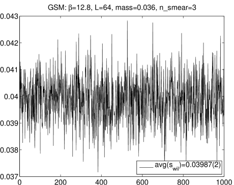
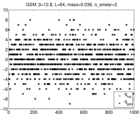
and Fig. 1 shows a part of the pertinent Monte-Carlo history of the plaquette action and of the topological charge on the finest lattice ($\beta\!=\!12.8$). The Wilson action per site is defined as $s_{\mathrm{wil}}(x)\!=\!1\!-\!\mathrm{Re}\,U_{12}(x)\!=\!1\!-\!\cos(\theta_{12})$ with $U_{12}(x)\!=\!U_{1}(x)U_{2}(x\!+\!e_{1})U_{1}^{\dagger}(x\!+\!e_{2})U_{2}^{\dagger}(x)\!=\!\exp(\mathrm{i}\theta_{12})$ denoting the plaquette. For the topological charge two field-theoretic definitions are used, $q_{\mathrm{nai}}^{(3)}\!=\!\sum\;\sin(\theta_{12}^{(3)})/(2\pi)\!\in\!\mathbf{R}$ (“naive”) and $q_{\mathrm{geo}}^{(3)}\!=\!\sum\;\theta_{12}^{(3)}/(2\pi)\!\in\!\mathbf{Z}$ (“geometric”), where $\theta_{12}^{(3)}$ denotes the plaquette angle after $3$ smearing steps. The algorithm is seen to tunnel well.

4 Staggered spectroscopy with all-to-all technology

In weak coupling perturbation theory staggered fermions have been proven to be sensitive to the axial anomaly [33, 34]. Still, it seems worth demonstrating that this sensitivity carries over, at the non-perturbative level, to the asymptotic states of the theory, and leads to a non-vanishing mass of the combined taste-and-flavor singlet pseudoscalar meson in the chiral limit.

The remnant staggered form of the continuum index theorem has been investigated in a classic paper [29]. A direct check of the mass excess of the $\eta$ ($\eta^{\prime}$) in $N_{\!f\,}\!=\!2$ ($N_{\!f\,}\!=\!3$) QCD with rooted staggered quarks and standard taste assignment has been attempted [35, 36, 37, 38], but unfortunately in the disconnected contributions the signal dies quickly in the noise [39, 40, 41, 42, 43, 44]. Encouraged by [27, 28], we now attack the same goal in the much simpler Schwinger model.

With a single staggered field, we expect to find 4 pseudoscalar bosons. The lightest ($\gamma_{5}\!\otimes\!\xi_{5}$, to be dubbed $\pi^{0}$) becomes massless (on an infinitely large lattice) in the limit $m\!\to\!0$, the next two ($\gamma_{5}\!\otimes\!\xi_{1}$ and $\gamma_{5}\!\otimes\!\xi_{1}\xi_{5}$, to be dubbed $\pi^{\pm}$) become massless up to cut-off effects, while the last one ($\gamma_{5}\!\otimes\!1$, to be dubbed $\eta$) is supposed to be well separated and stay massive in the chiral limit. In standard terminology, the $\pi^{0}$ is taste-pseudoscalar, the $\pi^{\pm}$ are taste-(axial)vector (in 2D there is no distinction), while the $\eta$ is taste-scalar (or taste-singlet) – see [4] for details.

Figure 2: Left: Correlation between the topological charges $q_{\mathrm{geo}}^{(3)}$ and $q_{\mathrm{stag}}^{(3)}$, based on the $\Gamma_{50}$ operator (5), with 3 smearings. Right: Overall topological charge distribution for $N_{\!f\,}\!=\!0$, and after reweighting to $N_{\!f\,}\!=\!1,2$. Either plot refers to the intermediate mass run at $\beta\!=\!7.2$.

Staggered spectroscopy is performed by constructing dedicated correlators which project to a specific spinor-taste combination. In phenomenological applications it is common practice to use a source at a single lattice point as a “broad band emitter” which couples to all spinor-taste combinations, and to apply the projection only at the sink. In this work, we use an all-to-all propagator technique, and shall apply spinor-taste projection independently at the source and the sink. In explicit terms, for the $\gamma_{5}\!\otimes\!\xi_{5}$ “Goldstone” state we use the operator $\Gamma_{55}=(-1)^{x_{1}+x_{2}}$, which is a point-like operator. By contrast, the operator $\Gamma_{50}\simeq(\gamma_{5}\!\otimes\!1)$ is defined by [29]

$$\Gamma_{50} = \frac{\mathrm{i}}{2}(\Gamma_{1}\Gamma_{2}-\Gamma_{2}\Gamma_{1})\quad\mbox{where}$$ (5)

$$\Gamma_{\mu}(x,y) = \frac{1}{2}\eta_{\mu}(x)\Big{[}U_{\mu}(x)\delta_{x+\hat{\mu},y}+U_{\mu}^{\dagger}(x\!-\!\hat{\mu})\delta_{x-\hat{\mu},y}\Big{]}$$ (6)

with $\eta_{\mu}(x)=(-1)^{\sum_{\nu<\mu}x_{\nu}}$, and is thus a 2-hop operator (it would be 4-hop in 4D).

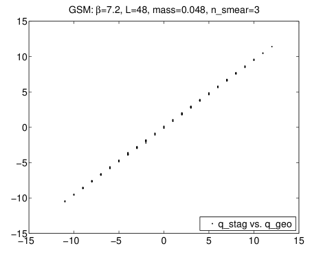
The operator (5) is supposed to be sensitive to the topological charge of the gauge background $U$, and to test our implementation we routinely determine the fermionic charge

$$q_{\mathrm{stag}}[U]=\frac{m}{2}\,\mathrm{tr}(G\Gamma_{50})$$ (7)

where $G$ denotes the Green’s function of the massive staggered operator. A scatter plot of (7) ($y$-axis) versus the gluonic charge $q_{\mathrm{geo}}[U]$ ($x$-axis) is shown in Fig. 2. We also checked that the operator $\Gamma_{50}\Gamma_{55}\simeq 1\!\otimes\xi_{5}$ is not sensitive to the topological charge.

With these projections it is straightforward to construct the connected $\pi^{0}$ and $\eta$ correlators

$$C_{\pi}(t) = \frac{1}{L^{2}}\sum_{x,y,x_{2}-y_{2}=t\,(\mathrm{mod}\,T)}G(x,y)\Gamma_{55}(y)G(y,x)\Gamma_{55}(x)$$ (8)

$$C_{\eta}(t) = \frac{1}{L^{2}}\sum_{x,y,x_{2}-y_{2}=t\,(\mathrm{mod}\,T)}G(x,y^{\prime})\Gamma_{50}(y^{\prime},y)G(y,x^{\prime})\Gamma_{50}(x^{\prime},x)$$ (9)

where $\delta(x^{\prime},x)\Gamma_{55}(x)\!=\!\Gamma_{55}(x^{\prime},x)$ is used, and the primed positions are implicitly summed over. For the combined taste-and-flavor singlet state there is also the disconnected contribution

$$D_{\eta}(t)\;=\;\frac{1}{L^{2}}\sum_{x,y,x_{2}-y_{2}=t\,(\mathrm{mod}\,T)}G(x,x^{\prime})\Gamma_{50}(x^{\prime},x)G(y,y^{\prime})\Gamma_{50}(y^{\prime},y)$$ (10)

and for staggered fermions it must be combined with (9) in the form [35]

$$F_{\eta}(t)\;\equiv\;\frac{N_{\!f\,}}{N_{t}}C_{\eta}(t)-\frac{N_{\!f\,}^{2}}{N_{t}^{2}}D_{\eta}(t)$$ (11)

to obtain the full 2-point function of the $\eta$ state. Here $N_{t}=2^{d/2}$ denotes the number of “tastes” of a staggered field in $d$ spacetime dimensions. Since $C_{\eta}(t)$ and $F_{\eta}(t)$ fall off exponentially, at large $t$, with masses $M_{\eta}^{\mathrm{conn}}$ and $M_{\eta}^{\mathrm{full}}$ respectively (where only the latter one is physical), it follows that the ratio of the disconnected over the connected correlator takes the form

$$R_{\eta}(t)\equiv\frac{D_{\eta}(t)}{C_{\eta}(t)}\;\longrightarrow\;\frac{N_{t}}{N_{\!f\,}}-\mathrm{const}\,\frac{e^{-M_{\eta}^{\mathrm{\;full\;}}t}+e^{-M_{\eta}^{\mathrm{\;full\;}}(T-t)}}{e^{-M_{\eta}^{\mathrm{conn}}t}+e^{-M_{\eta}^{\mathrm{conn}}(T-t)}}\;\simeq\;\frac{N_{t}}{N_{\!f\,}}-\mathrm{const}\,e^{-\Delta\!M_{\eta}\,t}$$ (12)

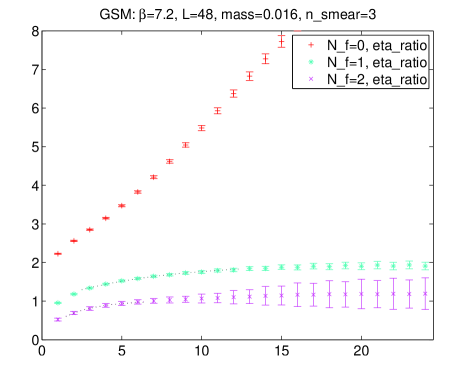
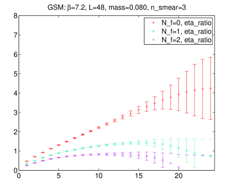
where $\Delta\!M_{\eta}\!\equiv\!M_{\eta}^{\mathrm{full}}\!-\!M_{\eta}^{\mathrm{conn}}$, and the simplification applies for $a\!\ll\!t\!\ll\!T$. In other words, the prediction is that in 2D the ratio (12) levels off at 2 for $N_{\!f\,}\!=\!1$, and at 1 for $N_{\!f\,}\!=\!2$.

5 Telling Goldstone bosons from non-Goldstone bosons

Figure 3: $aM_{\mathrm{eff}}(t)$ of $C_{\pi}(t)$ (left) and $C_{\eta}(t)$ (right), at $\beta\!=\!7.2$ for the intermediate quark mass.

Figure 4: Correlation between the disconnected $D_{\eta}(t)$ and the squared topological charge $q_{\mathrm{geo}}^{(3)}$ for $t\!=\!T/4$ (left) and $t\!=\!T/2$ (right). Data are from the intermediate quark mass run at $\beta\!=\!7.2$.

Figure 5: Ratio $R_{\eta}(t)$ (12) at $\beta\!=\!7.2$ for the smallest (left) and largest (right) quark mass.

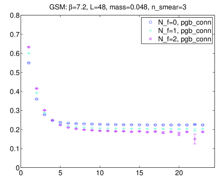
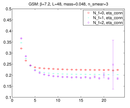
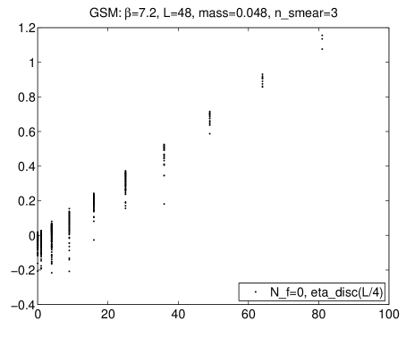
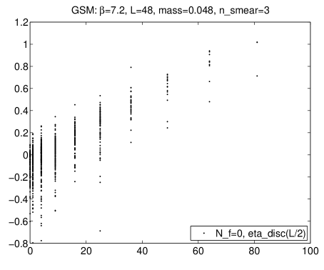
With the lattices of Tab. 1 in hand it is advisable to first check how well the different topological charges agree, how well the overall distribution is sampled, and whether the disconnected piece $D_{\eta}(t)$ is indeed sensitive to the overall charge of the background $U$.

The correlation between any pair of the three topological charges considered is very good; for the larger two $\beta$ even the $Z$-factor inherent in $q_{\mathrm{nai}}^{\mathrm{ren}}$ and $q_{\mathrm{stag}}^{\mathrm{ren}}$ is extremely close to 1, as can be inferred from Fig. 2. For $N_{\!f\,}\!=\!0$ the overall topological charge distribution is nicely sampled and close to a Gaussian. Under reweighting to $N_{\!f\,}\!=\!1$ or $N_{\!f\,}\!=\!2$ tiny asymmetries seem to get considerably enhanced. A feature relevant in what follows is that the dynamical distributions are narrower than the quenched one; with observables which are sensitive to topology it is useful to have the tails “oversampled” and to reduce their weight in the analysis.

After these checks have been carried out successfully, it is straightforward to determine the pion mass $aM_{\pi}$ for all couplings and quark masses. To this aim we consider the effective mass

$$aM_{\pi}(t)=\frac{1}{2}\log([C(t\!-\!1)+\sqrt{C(t\!-\!1)^{2}-C(T/2)^{2}}]/[C(t\!+\!1)+\sqrt{C(t\!+\!1)^{2}-C(T/2)^{2}}])$$ (13)

with $C\!\equiv\!C_{\pi}$, which is designed to compensate for the influence of the periodic boundary conditions. A typical example is shown in Fig. 3. A nice plateau is observed; albeit with tiny oscillations which grow towards the center of the box. Under reweighting to $N_{\!f\,}\!=\!1$ or $N_{\!f\,}\!=\!2$ this effect gets enhanced. For the connected piece of the eta (which is an unphysical state) similar results are obtained. Throughout, the difference between these two masses is tiny.

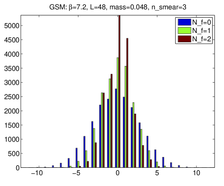
Turning to the disconnected piece $D_{\eta}(t)$, we first consider its correlation with the topological charge of the background. Example results are presented in Fig. 4. For these $t$ the sub-ensemble average $\langle D_{\eta}(t)\rangle_{q}$ seems to be a linear function of $q^{2}$ (which, from a glimpse at (10) and the definition of $q_{\mathrm{stag}}[U]$ is plausible). The issue most relevant is whether reasonable results for the disconnected-over-connected ratio (12) are obtained. Typical results are presented in Fig. 5. We obtain a rather clear signal up to about $t\!=\!T/4$ and find a qualitatively different behavior for the three $N_{\!f\,}$ shown. In the quenched case the pattern is consistent with a linear rise (with a slope which clearly depends on the quark mass). After reweighting to $N_{\!f\,}\!=\!1$ or $N_{\!f\,}\!=\!2$ the behavior is consistent with the prediction (12). A typical problem with the disconnected piece is that at large $t$ the data may go astray without the statistical error giving a hint of this (we tried several jackknife blocksizes). Still, we can extract the mass gap $a\Delta\!M_{\eta}$ from a fit to (12) at intermediate $t$, i.e. before the noise prevails. The results such obtained are collected in Tab. 2, along with the $aM_{\pi}$ values determined previously.

					$aM_{\pi}$					$a\Delta\!M_{\eta}$
$\beta$	$L/a$	$N_{\!f\,}$	$m_{1}$	$m_{2}$	$m_{3}$	$m_{4}$	$m_{5}$	$m_{1}$	$m_{2}$	$m_{3}$	$m_{4}$	$m_{5}$
1.8	24	0	0.279(01)	0.368(01)	0.444(01)	0.513(01)	0.579(01)	—	—	—	—	—
		1	0.220(01)	0.318(01)	0.402(01)	0.478(01)	0.550(01)	0.39(02)	0.36(07)	0.33(03)	0.31(04)	0.30(05)
		2	0.199(06)	0.292(02)	0.374(02)	0.454(01)	0.530(01)	0.83(42)	1.05(60)	0.63(08)	0.57(14)	0.53(21)
3.2	32	0	0.215(01)	0.281(01)	0.337(01)	0.389(01)	0.439(01)	—	—	—	—	—
		1	0.166(01)	0.240(01)	0.304(01)	0.362(01)	0.417(01)	0.28(02)	0.22(01)	0.21(01)	0.21(01)	0.18(01)
		2	0.154(07)	0.217(04)	0.283(01)	0.342(01)	0.400(01)	1.41(97)	0.48(02)	0.39(06)	0.36(02)	0.40(06)
7.2	48	0	0.142(01)	0.186(01)	0.224(01)	0.260(01)	0.294(01)	—	—	—	—	—
		1	0.111(02)	0.159(01)	0.203(01)	0.242(01)	0.279(01)	0.17(02)	0.14(01)	0.12(01)	0.11(01)	0.12(03)
		2	0.091(16)	0.137(06)	0.188(02)	0.230(01)	0.269(01)	0.45(07)	0.29(02)	0.28(01)	0.24(02)	0.22(02)
12.8	64	0	0.107(01)	0.140(01)	0.169(01)	0.196(01)	0.221(01)	—	—	—	—	—
		1	0.087(02)	0.123(01)	0.153(01)	0.183(01)	0.210(01)	0.14(02)	0.12(01)	0.10(02)	0.09(01)	0.09(02)
		2	0.086(07)	0.114(02)	0.143(02)	0.175(01)	0.201(02)	0.32(05)	0.24(04)	0.23(02)	0.19(01)	0.17(02)
3.2	24	0	0.231(01)	0.285(01)	0.338(01)	0.390(01)	0.439(01)	—	—	—	—	—
		1	0.182(01)	0.246(01)	0.306(01)	0.363(01)	0.416(01)	0.26(01)	0.23(01)	0.21(01)	0.19(01)	0.18(01)
		2	0.173(02)	0.229(01)	0.288(01)	0.346(01)	0.400(01)	2.12(1.56)	0.64(16)	0.47(02)	0.37(04)	0.33(05)
3.2	40	0	0.214(01)	0.280(01)	0.337(01)	0.389(01)	0.439(01)	—	—	—	—	—
		1	0.158(02)	0.241(01)	0.302(01)	0.363(01)	0.417(01)	0.28(13)	0.26(03)	0.21(02)	0.18(03)	0.21(04)
		2	0.138(04)	0.220(04)	0.276(05)	0.347(02)	0.402(01)	2.75(2.72)	1.23(83)	0.41(25)	0.38(12)	0.36(04)

Table 2: Measured $aM_{\pi}$ (Goldstone boson) and $a\Delta\!M_{\eta}$ (excess of the taste-and-flavor singlet pseudoscalar state) for all $\beta$, $L/a$, $N_{\!f\,}$, and $m$. The quark masses are given in Tab. 1.

The lower part of Tab. 2 contains the results of a finite-volume scaling study at $\beta\!=\!3.2$ (since finite volume effects relate to infrared physics the restriction to one $\beta$ is permissible). It seems that in the extra-small volume the pion mass is affected for the lightest two quark mass values. In the standard volume only the lightest quark mass data suffer from small finite volume artefacts. In case of the mass gap $a\Delta\!M_{\eta}$ no finite volume effects are found for $N_{\!f\,}\!=\!1$, while for $N_{\!f\,}\!=\!2$ the quality of the data is less convincing, which likely indicates the limitations of the reweighting method (fortunately, we are mostly interested in $a\Delta\!M_{\eta}$ for $N_{\!f\,}\!=\!1$).

Figure 6: Continuum extrapolation of $M_{\pi}/e$ ($N_{\!f\,}\!=\!2$, left) and $\Delta\!M_{\eta}/e$ ($N_{\!f\,}\!=\!1$, right) versus $a^{2}$.

Figure 7: Chiral extrapolation of $(M_{\pi}/e)^{3}$ versus $(m/e)^{2}$ (left) and $\Delta\!M_{\eta}/e$ versus $m/e$ (right).

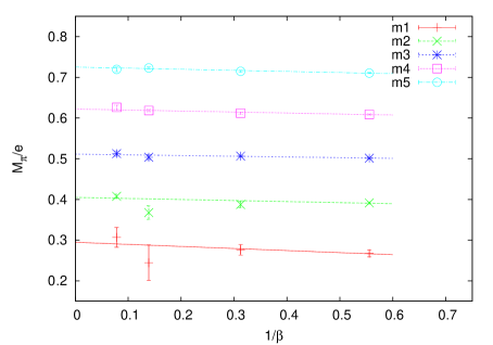
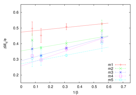
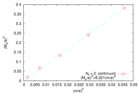
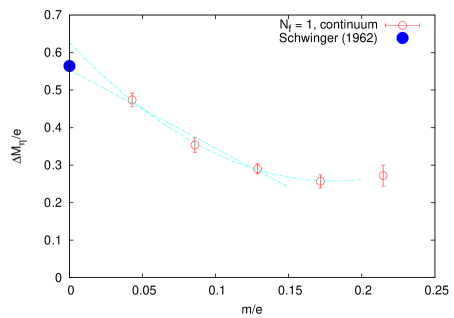
The next step is a continuum extrapolation of the meson masses obtained. We do this both for $M_{\pi}/e$ in the $N_{\!f\,}\!=\!2$ theory (to test the prediction by Smilga [25], see above) and for the main object of interest $\Delta\!M_{\eta}/e$ in the $N_{\!f\,}\!=\!1$ theory. As mentioned in Sec. 2 the simulations were carried out at fixed physical quark masses (i.e. $m/e$), such that the data of Tab. 2 can be continuum extrapolated without interpolation in $m$. These extrapolations are shown in Fig. 6. It seems that all four lattice spacings are in the Symanzik scaling regime; we obtain acceptable linear fits with two degrees of freedom.

With these continuum results for $M_{\pi}/e$ (for $N_{\!f\,}\!=\!2$) and $\Delta\!M_{\eta}/e$ (for $N_{\!f\,}\!=\!1$) in hand, it is interesting to consider their quark mass dependence. In the left panel of Fig. 7 we plot $(M_{\pi}/e)^{3}$ as a function of $(m/e)^{2}$. Here, the lightest pion mass has been adjusted by the finite volume correction factor $0.138/0.154\!=\!0.896$ (taken from Tab. 2). Using a 1-parameter ansatz fits the data with $\chi^{2}/\mathrm{d.o.f}\!=\!1.13$ and a slope parameter of $8.221(63)$. This is in reasonable agreement with Smilga’s prediction that this parameter should be $2.008^{3}\!=\!8.096$ [25].

Last but not least let us consider the quark mass dependence of the mass gap $\Delta\!M_{\eta}/e$ in the $N_{\!f\,}\!=\!1$ theory, as shown in the right panel of Fig. 7. Being unaware of an analytic prediction, it is not entirely clear which powers of $\Delta\!M_{\eta}/e$ and $m/e$ one should choose to display the data, and we opt for staying without additional powers. Fortunately, in this representation the quark mass dependence seems mild, and both a linear and a quadratic fit with one degree of freedom describe the data convincingly. Taking half of the spread as the systematic error, these fits predict $\Delta\!M_{\eta}/e=0.591(25)(37)$ in the chiral limit, which is in perfect agreement with Schwinger’s analytic result $M_{\eta}/e=\Delta\!M_{\eta}/e=1/\sqrt{\pi}=0.56419$ [24].

6 Summary

Triggered by the criticism of [5, 6, 7] the validity of the “rooting trick” in studies with staggered quarks has been the subject of an intense debate in the lattice community. Several review talks at major conferences [8, 9, 10, 11] presented a wealth of numerical and analytical evidence in favor of the procedure, but so far the “experimentum crucis”, i.e. a direct test of $\eta^{\prime}$-phenomenology in QCD with rooted staggered quarks remained elusive, due to noise issues [35, 36, 37, 38].

This paper is based on the observation that there is no strict need to investigate the topic in QCD, since the conceptual issue is one-to-one matched in the massive Schwinger model with 1 flavor, which is much simpler to simulate. We demonstrated that in this case it is possible to obtain conclusive results for the disconnected-over-connected ratio (12). As shown in Fig. 5 the prediction (12) with $N_{\!f\,}\!=\!1$ and $N_{t}\!=\!2$ is beautifully confirmed. In consequence the mass gap $\Delta\!M_{\eta}$ or the physical mass $M_{\eta}$ in the 1-flavor theory can be determined with sufficient precision, so that a combined continuum and chiral extrapolation is possible. The result is in perfect agreement with the analytical prediction $M_{\eta}\!=\!e/\sqrt{\pi}$ by Schwinger [24].

It seems this is the first ad oculos demonstration that the staggered setup – with the rooting trick in the functional measure – treats the contribution of the axial anomaly to the particle spectrum correctly. With this result, and in view of [35, 36, 37, 38], one may predict that the outcome of a similar study in QCD will be identical, once sufficient CPU power is available.

Acknowledgments: It is a pleasure to acknowledge useful correspondence with Steve Sharpe, Claude Bernard and Zoltán Fodor. Partial support was provided by Bern University, DESY Zeuthen, and through SFB/TR-55. Computations were performed on a stand-alone PC at JSC.

References

- [1]
- [2] L. Susskind, Phys. Rev. D 16, 3031 (1977).
- [3] E. Marinari, G. Parisi and C. Rebbi, Nucl. Phys. B 190, 734 (1981).
- [4] A. Bazavov et al. [MILC Collab.], Rev. Mod. Phys. 82, 1349 (2010) [arXiv:0903.3598].
- [5] K. Jansen, Nucl. Phys. Proc. Suppl. 129, 3 (2004) [hep-lat/0311039].
- [6] M. Creutz, Phys. Lett. B 649, 230 (2007) [hep-lat/0701018].
- [7] M. Creutz, PoS LAT2007, 007 (2007) [arXiv:0708.1295].
- [8] S. Dürr, PoS LAT2005, 021 (2006) [hep-lat/0509026].
- [9] S. R. Sharpe, PoS LAT2006, 022 (2006) [hep-lat/0610094].
- [10] A. S. Kronfeld, PoS LAT2007, 016 (2007) [arXiv:0711.0699].
- [11] M. Golterman, PoS CONFINEMENT 8, 014 (2008) [arXiv:0812.3110].
- [12] V. Azcoiti et al., Phys. Rev. D 50, 6994 (1994) [hep-lat/9401032].
- [13] S. Dürr and C. Hoelbling, Phys. Rev. D 69, 034503 (2004) [hep-lat/0311002].
- [14] S. Dürr and C. Hoelbling, Phys. Rev. D 71, 054501 (2005) [hep-lat/0411022].
- [15] E. Follana et al., Phys. Rev. Lett. 93, 241601 (2004) [hep-lat/0406010].
- [16] S. Dürr, C. Hoelbling and U. Wenger, Phys. Rev. D 70, 094502 (2004) [hep-lat/0406027].
- [17] E. Follana et al., Phys. Rev. D 72, 054501 (2005) [hep-lat/0507011].
- [18] D. H. Adams, Phys. Rev. Lett. 104, 141602 (2010) [arXiv:0912.2850].
- [19] S. R. Sharpe and R. S. Van de Water, Phys. Rev. D 71, 114505 (2005) [hep-lat/0409018].
- [20] C. Bernard, Phys. Rev. D 73, 114503 (2006) [hep-lat/0603011].
- [21] C. Bernard, M. Golterman, Y. Shamir, Phys. Rev. D 73, 114511 (2006) [hep-lat/0604017].
- [22] Y. Shamir, Phys. Rev. D 75, 054503 (2007) [hep-lat/0607007].
- [23] G. C. Donald et al., Phys. Rev. D 84, 054504 (2011) [arXiv:1106.2412].
- [24] J. S. Schwinger, Phys. Rev. 128, 2425 (1962).
- [25] A. V. Smilga, Phys. Rev. D 55, 443 (1997) [hep-th/9607154].
- [26] C. B. Lang and T. K. Pany, Nucl. Phys. B 513, 645 (1998) [hep-lat/9707024].
- [27] H. Fukaya and T. Onogi, Phys. Rev. D 68, 074503 (2003) [hep-lat/0305004].
- [28] W. Bietenholz, I. Hip, S. Shcheredin and J. Volkholz, arXiv:1109.2649 [hep-lat].
- [29] J. Smit and J. C. Vink, Nucl. Phys. B 286, 485 (1987).
- [30] N. Metropolis et al., J. Chem. Phys. 21, 1087 (1953).
- [31] F. R. Brown and T.J. Woch, Phys. Rev. Lett. 58, 2394 (1987).
- [32] D. B. Leinweber et al., Phys. Lett. B 585, 187 (2004) [hep-lat/0312035].
- [33] L. H. Karsten and J. Smit, Nucl. Phys. B 183, 103 (1981).
- [34] H. S. Sharatchandra, H. J. Thun and P. Weisz, Nucl. Phys. B 192, 205 (1981).
- [35] L. Venkataraman and G. Kilcup, hep-lat/9711006.
- [36] E. B. Gregory et al., Phys. Rev. D 77, 065019 (2008) [arXiv:0709.4224].
- [37] E. B. Gregory et al., PoS LATTICE 2008, 286 (2008) [arXiv:0810.0136].
- [38] E. B. Gregory et al., arXiv:1112.4384 [hep-lat].
- [39] T. Struckmann et al. [TXL Collab.], Phys. Rev. D 63, 074503 (2001) [hep-lat/0010005].
- [40] V. I. Lesk et al. [CP-PACS Collab.], Phys. Rev. D 67, 074503 (2003) [hep-lat/0211040].
- [41] K. Schilling, H. Neff and T. Lippert, Lect. Notes Phys. 663, 147 (2005) [hep-lat/0401005].
- [42] K. Hashimoto and T. Izubuchi, Prog. Theor. Phys. 119, 599 (2008) [arXiv:0803.0186].
- [43] N. H. Christ et al., Phys. Rev. Lett. 105, 241601 (2010) [arXiv:1002.2999].
- [44] K. Ottnad, C. Urbach, C. Michael and S. Reker, arXiv:1111.3596 [hep-lat].
- [45] C. Bernard and M. Golterman, PoS LATTICE 2010, 252 (2010) [arXiv:1011.0184].