Potential vorticity dynamics in the framework of disk shallow-water theory: II. Mixed Barotropic-Baroclinic Instability

Abstract

Context. Potential vorticity dynamics for astrophysical disks.

Aims. Extend exploration of these instabilities in cold astrophysical disks which are three dimensional whose mean states are baroclinic. In particular, we seek to demonstrate the potential existence of traditional baroclinic instabilities of meteorological studies. We show this in a simplified two-layer Philips Disk Model of a midplane symmetric disk.

Methods. We consider the dynamical normal-mode response of thin annular disks with two potential vorticity defects, one in each of two disk layers. Each disk layer is of constant but differing densities. The resulting mean azimuthal velocity profile shows a variation in the vertical direction implying that the system is baroclinic in the mean state. The stability of the system is treated in the context of disk shallow water theory wherein azimuthal disturbances are much longer than the corresponding radial or vertical scales. The normal-mode problem is solved numerically using two different methods.

Results. The results of a symmetric single layer barotropic model is considered and it is found that instability persists for models in which the potential vorticity profiles are not symmetric, consistent with previous results. The instaiblity is interpreted in terms of interacting Rossby waves. For a two layer system in which the flow is fundamentally baroclinic we report here that instability takes on the form of mixed barotropic-baroclinic type: instability occurs but it qualitatively follows the pattern of instability found in the barotropic models. Instability arises because of the phase locking and interaction of the Rossby waves between the two layers. The strength of the instability weakens as the density contrast between layers increases.

Conclusions. Baroclinic instability is feasible for astrophysical disks but has the character of mixed barotropic-baroclinic type. The instability as explored in this study could be present in protoplanetary disks with weak vertical density stratification.

1 Introduction

The phenomenon of baroclinic instability has been studied with intensity for over 70 years. Sometimes referred to as sloping convection (Vallis 2006), it is an instability that relies on the presence of a vertical shear in a zonal flow in a rotating atmosphere. This archetypical sheared flow exists as a result of a thermal-wind relationship balancing Coriolis effects with meridional (equator-to-pole) temperature gradients. It is ultimately a reflection of the mismatch in the isobars and isopycnals in an atmosphere. It is alternatively interpreted as an instability resulting from the interaction of inter-layer Rossby waves (Hoskins et al. 1985, Baines and Mitsudera 1994, Heifetz 2004). Baroclinic instability is important to a variety of geophysical and astrophysical phenonomena. Among others, it plays a well-known role in the generation of terrestrial weather as well as in the dynamics of the Ocean Mixed Layer (Haine and Marshall 1998). It has been conjectured to play an important role in the mixing processes in stars (Knobloch and Spruit 1982, Fujimoto 1988).

The original studies of the instability (e.g. Charney 1947, Eady 1949, Philips 1954) considered the process in the small Rossby number limit in which the Rossby number, Ro, is given by ${\cal U}/2\Omega_{0}{\cal L}$, where the terms are (respectively) the typical speed of a vortex, planetary rotation rate (at latitude) and the typical horizontal length scale of the flow. Baroclinic instability is a process that figures prominently in the geostrophic limit (Ro $\ll 1$) but theoretical considerations have shown that it persists relatively unabated even when Ro is $\sim 1$ (Stone 1970, Stone 1971, Molemaker et al. 2005). These studies also argue that the instability also persists for significant deviations from hydrostasy.

The possibility that baroclinic instability is present in accretion disk flows, which are characterized by Ro $=0.75$, was examined in the studies of Cabot (1984) and Knobloch and Spruit (1985,1986). Owing to the fundamental inseparability of the resulting linearized problem (even in the relatively simplified Boussinesq limit) Knobloch and Spruit (1986) were only able to conclude that the instability is feasible for radial and vertical disturbances comparable to the local scale height of the disk. The feature complicating the analysis and rendering it inseparable is the dominance of the Keplerian shear making traditionally employed small Ro analyses of meteorological studies here unusable.

Adding to the challenge: because the Keplerian shear is barotropic the resulting problem for a disk is fundamentally of mixed baroclinic-barotropic type. This type of mixed problem has been examined in the context of quasigeostrophic flows by McIntyre (1970), Ioannou & Lindzen (1986), James (1987). These studies generally agree that the structure of baroclinic waves will get increasingly confined in the shearwise direction with increasing strength of the barotropic shear. The confinement, due to the barotropic governor mechanism (James 1987), appears to have the effect of weakening growth rates.

Keplerian disks are notoriously difficult to finesse into a geostrophic-hydrostatic framework familiar in traditional meteorology. Knobloch and Spruit (1985,1986) note that it is only in the long stremwise wavelength limit (azimuthal in disk geometry) of a Keplerian flow will some of the formalism of quasigeostrophy carry over. Umurhan (2008) developed a scaling analysis in which a local annular disk section can be viewed in a semi-geostrophic, quasi-hydrostatic framework (see also Balmforth and Spiegel 1996). This, in turn, permits a dynamical analysis purely in terms of the potential vorticity, typical of meteorological studies. This construction was used to re-examine the Rossby wave instability (Li et al. 2000, Meheut et al. 2010) by illustrating it in a setting stripped down to its essential components (Umurhan 2010).

We use the limit developed in Umurhan (2008) to examine baroclinic instability in an annular section of a cold accretion disk. We circumvent the difficulties encountered in Knobloch and Spruit’s calculation by constructing a two-layer Philips model (Philips 1954). The Philips model is an effective simplification of the governing equations that allows for analytical tractability without losing the underlying physics at play in the baroclinic instability (see an extended discussion of this in the text of Vallis 2006).

This work is organized as follows. In Section 2 we develop a two-layer Philips disk model from the disk shallow water equations found in Umurhan (2008) utilyzing a number of simplifications and assumptions. In Section 3 we set up the general normal mode problem for this two-layer, mid-plane symmetric, model system including the boundary conditions and numerical methods employed. We describe the model whose stability we test including a description of the features we include which is designed to strip away the complications arising from critical layers. In Section 4 we consider the stability properties of a purely barotropic (single-layer) configuration and interpret the results from the perspective of interacting Rossby waves developed in previous studies. In Section 5 we build upon the picture developed for the barotropic calculation and describe a baroclinic model configuration and examine its stability properties. In Section 6 we offer a summary of our principle results and a short litany of reflections and remarks.

2 Derivation of the Two-Layer Philips Disk Model

Figure 1: Configuration of two layer Philips Model.

The analysis of this study assumes dynamics occur on azimuthal length scales which are much longer than the system’s vertical and radial scales. The equations appropriate for such a thin annular setting were developed from a scaling analysis detailed in Umurhan (2008). However they can be found in various other forms in older studies as well, e.g. Knobloch and Spruit (1985,1986) and Balmforth and Spiegel (1996).

These equations describe dynamics in a thin annular section of a disk centered at some radius $R$ rotating with the local Keplerian rate $\Omega_{K}=\sqrt{GM/R^{3}}$. If the local soundspeed of the disk is given by $c_{s}$ then the ratio $\varepsilon=c_{s}/(R\Omega_{K})$ forms a natural small parameter of the disk equations. Formally this means we will take $\varepsilon\ll 1$. The equations are therefore derived by assuming a number of scalings, namely that the azimuthal velocity scales as $c_{s}$ and that the vertical and radial velocities scale as $\varepsilon c_{s}$. Together with the assumption that the radial and vertical scales are a factor of $\varepsilon$ smaller than the azimuthal scale $R$, the velocity assumptions here imply a long time scale ${\cal T}\sim 1/\varepsilon\Omega_{K}$. It is important to note that this long timescale necessarily filters out acoustic and gravity wave type motions from these dynamics. The combination of these scalings into the fundamental equations of motion results in the following set of reduced non-dimensionalized equations

$$-2\Omega_{0}V = -\frac{1}{\rho}\partial_{x}P-q\Omega_{0}^{2}x,$$ (1)

$$\frac{dV}{dt}+2\Omega_{0}u = -\frac{1}{\rho}\partial_{y}P,$$ (2)

$$0 = -\frac{1}{\rho}\partial_{x}P+\Omega_{0}^{2}z,$$ (3)

together with

$$\frac{1}{\rho}\frac{d\rho}{dt}+\nabla\cdot{{\bf u}} = 0,$$ (4)

$$\rho T\frac{dS}{dt} = {\cal{Q}},$$ (5)

in which

$$\frac{d}{dt}=u\partial_{x}+V\partial_{y}+w\partial_{z}.$$

$P=\rho T$ is the pressure, where $\rho$ and $T$ respectively denote density and temperature. The velocity vector ${\bf u}=(u,V,w)$ is comprised of components in the radial ($x$), azimuthal ($y$) and disk vertical ($z$) directions respectively. The lengths $x$ and $z$ represent the radial and vertical scales scaled by $\varepsilon R$ while the azimuthal scales $y$ being scaled by $R$. The entropy is $S\equiv\ln P/\rho^{\gamma}$ where $\gamma$ is the ratio of specific heats. $\Omega_{0}$ represents the non-dimensionalization of the usual Coriolis terms that emerge when one moves into a rotating frame. In this formulation it is formally ‘$1$’ but we keep it around for the sake of latter clarity. For Keplerian disk systems $q=3/2$.

The lack of the usual inertial terms in the resulting radial and vertical momentum equations expresses the extremeness of the scalings describing the thin annular disk region. The resulting equations describe dynamics which are vertically hydrostatic but, moreover, geostrophic in the radial direction. In meteorological studies this is sometimes referred to as semi-geostrophic because the azimuthal flow dynamics are not in fundamental geostrophic balance.

To derive a Philips model that is tractable and transparent the following assumptions are made:

1. Dynamics are symmetric about the midplane $z=0$,

2. Two layers are examined with differing uniform densities (and the configuration is stable to buoyant instabilities),

3. The flow in each layer is incompressible.

The assumption of incompressibility means that the continuity equation is replaced, instead, by

$$\nabla\cdot{\bf u}=0,$$ (6)

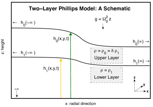
in each layer. A pictoral representation of the system envisioned for this analysis is shown in Figure 1. From here on forth, quantities in the upper layer are designated with a subscript ‘$0$’ while in the lower layer they are represented by the subscript ‘$1$’. Thus, for example, the uniform density of the upper layer is $\rho_{0}$ while in the lower layer it is $\rho_{1}$. Because incompressibility has been assumed for each layer there is no longer any need for the energy equation (5). Instead, the evolution of each layer’s thickness will be followed (see below).

A qualitative inspection of the state of affairs depicted in Figure 1 shows that, indeed, the isopycnals and isobars of the atmosphere are misaligned which means that the basic state will be baroclinic with the in-layer azimuthal velocities being different from one another. The misalignment has been placed here by hand and is controlled by the functional form of the heights $h_{0}$ and $h_{1}$. The origins of their respective distributions ultimately rests upon radially dependent thermal process involving radiation and disk chemistry requiring detailed calculations (e.g. Turner et al. 2012) without making the simplifying assumptions we have made. For the purpose of this model, how the atmosphere got arranged into this configuration is not our concern: it is enough that the profile is in steady state.

The azimuthal velocity in both layers are written as a sum of the local Keplerian part $-q\Omega_{0}x$ plus a deviation $v_{i}$ where $i$ is either ‘$0$’ or ‘$1$’ as in, $V_{i}=-q\Omega_{0}x+v_{i}$. Assuming that the pressure of the disk is zero at its top, the vertical momentum equation may be immediately integrated to yield,

$$P=\Omega_{0}^{2}\frac{1}{2}\left\{\begin{array}[]{ll}\rho_{0}(h_{0}^{2}-z^{2});&h_{1}\leq z\leq h_{0},\\ &\\ \rho_{0}(h_{0}^{2}-h_{1}^{2})+\rho_{1}(h_{1}^{2}-z^{2});&0\leq z\leq h_{1}.\end{array}\right.$$ (7)

Putting this solution for the pressure back into the horizontal momentum equations shows that for each layer

$$-2\Omega_{0}v_{i} = -\partial_{x}\Pi_{i},$$ (8)

$$\left(\frac{D}{Dt}\right)_{i}v_{i}+\Omega_{0}(2-q)u_{i} = -\partial_{y}\Pi_{i},$$ (9)

where

$$\Pi_{0}=\frac{1}{2}\Omega_{0}^{2}h_{0}^{2},\qquad\Pi_{1}=\frac{1}{2}\Omega_{0}^{2}\Bigl{[}\delta h_{0}^{2}+(1-\delta)h_{1}^{2}\Bigr{]}.$$ (10)

The quantity $\Pi_{i}$ may be viewed as the analog of the streamfunction in meteorological studies. Each layer height, which is in effect an integration constant, is designated by $h_{i}(x,y,t)$. The parameter $\delta\equiv\rho_{0}/\rho_{1}$ measures the ratio of the two densities. Henceforth, since interest is in configurations which are buoyantly stable, attention will be given only to those values of $\delta<1$.

Inspection reveals that the resulting horizontal momentum equations are independent of the vertical coordinate. As such the time derivative operator in each layer has been written as

$$\left(\frac{D}{Dt}\right)_{i}=\partial_{t}+u_{i}\partial_{x}+(v_{i}-q\Omega_{0}x)\partial_{y}.$$

The incompressiblity equations may be integrated in each layer revealing

$$w=\left\{\begin{array}[]{ll}-z(\partial_{x}u_{0}+\partial_{y}v_{0})+\bar{W}_{0};&h_{1}\leq z\leq h_{0},\\ &\\ -z(\partial_{x}u_{1}+\partial_{y}v_{1});&0\leq z\leq h_{1}.\end{array}\right.$$ (11)

The symmetry condition has been imposed upon the vertical velocity profile by enforcing that its value is zero at $z=0$. The velocity term $\bar{W}_{0}$ is determined by enforcing certain matching conditions when following the motion of the individual interfaces. Since $\bar{W}_{0}$ plays no essential role in the subsequent linear theory we do not detail its form here. The motion of each layer edge is viewed from both layers and is accordingly set equal to the vertical velocities found in (11). Combining this with the criterion that there is no layer separation reveals that the dynamics of each layer’s thickness is governed by

$$\left(\frac{D}{Dt}\right)_{1}h_{1}=-(\partial_{x}u_{1}+\partial_{y}v_{1})h_{1},$$ (12)

and

$$\left(\frac{D}{Dt}\right)_{0}(h_{0}-h_{1})=-(\partial_{x}u_{0}+\partial_{y}v_{0})(h_{0}-h_{1}).$$ (13)

The above equations may be combined and simplified following standard procedures resulting in

$$\left(\frac{DQ_{0}}{Dt}\right)_{0}=0,\qquad Q_{0}\equiv\frac{\Omega_{0}(2-q)+\partial_{x}v_{0}}{h_{0}-h_{1}},$$ (14)

in the upper layer while, for the lower layer,

$$\left(\frac{DQ_{1}}{Dt}\right)_{1}=0,\qquad Q_{1}\equiv\frac{\Omega_{0}(2-q)+\partial_{x}v_{1}}{h_{1}}.$$ (15)

The above relate the fact that the potential vorticities in each layer, represented by $Q_{0}$ and $Q_{1}$, are materially conserved by the flow. It should be noted here that even though the $Q_{i}$ are conserved in each of their respective layers, because the same $Q_{i}$ involve quantities that develop in layers outside of their own means that layers are coupled to one another.

Equations (14-15) together with (8-10) completely describe the model system. It is referred to hereafter as the two-layer Philips disk model.

3 Steady states, their perturbations and numerical method

As the purpose of this work is to demonstrate the possible normal-mode responses for various configurations of this two-layer Philips model, in this section we develop the formalism for the perturbative study of generalized steady state configurations. This steady states are assumed to be radially dependent, however, perturbations of these states are non-axisymmetric. In the subsequent two sections we will detail the normal mode response for a variety of specific steady state profiles.

For the sake of transparency in the following presentation $\Omega_{0}$ shall be set to its nominal value of $1$. We study perturbations of already laid down potential vorticity profiles. These steady profiles describe mean azimuthal velocities which are deviations around the Keplerian base flow. There are no mean radial velocities. This means in effect, that the mean PV profiles will depend only upon the radial coordinate $x$. Therefore, assuming $Q_{0}=\bar{Q}_{0}(x)$ and $Q_{1}=\bar{Q}_{1}(x)$ it follows from the relationships between $Q_{i}$’s and $\Pi_{i}(h_{0},h_{1})$ found in (14-15) that

$${2(2-q)+\partial_{x}^{2}\bar{\Pi}_{0}}-2\bar{Q}_{0}{(\bar{h}_{0}-\bar{h}_{1})} = 0,$$ (16)

$$2(2-q)+\partial_{x}^{2}\bar{\Pi}_{1}-2\bar{Q}_{1}\bar{h}_{1} = 0,$$ (17)

in which the relationships between $\Pi$ and $h_{i}$, found in (10), have been inverted:

$$\bar{h}_{0}=(2\bar{\Pi}_{0})^{1/2},\qquad\bar{h}_{1}=2^{1/2}\left(\frac{\bar{\Pi}_{1}-\delta\bar{\Pi}_{0}}{1-\delta}\right)^{1/2};$$ (18)

expressing the mean steady height’s $\bar{h}_{i}$ in terms of the steady in-layer pressures $\bar{\Pi}_{i}$. In deriving the above expressions the following relationships have also been explicitly used,

$$\bar{v}_{0}=\frac{1}{2}\partial_{x}^{2}\bar{\Pi}_{0},\qquad\bar{v}_{1}=\frac{1}{2}\partial_{x}^{2}\bar{\Pi}_{1}.$$ (19)

Linear perturbations of the Philips model system developed by writing for all dependent quantities ‘$f$’

$$F_{i}\rightarrow\bar{F}_{i}(x)+F_{i}^{\prime}(x,y,t)$$ (20)

where the primes denote perturbations. Equations (14-15) and (8-10) are explicitly written out

$$(\partial_{t}+\bar{v}_{0}\partial_{y}-qx\partial_{y})Q_{0}^{\prime}+u_{0}^{\prime}\partial_{x}\bar{Q}_{0} = 0,$$ (21)

$$(\partial_{t}+\bar{v}_{1}\partial_{y}-qx\partial_{y})Q_{1}^{\prime}+u_{1}^{\prime}\partial_{x}\bar{Q}_{1} = 0,$$ (22)

in which

$$(\bar{h}_{0}-\bar{h}_{1})Q_{0}^{\prime} = \partial_{x}v_{0}^{\prime}-\bar{Q}_{0}(h_{0}^{\prime}-h_{1}^{\prime}),$$ (23)

$$\bar{h}_{1}Q_{1}^{\prime} = \partial_{x}v_{1}^{\prime}-\bar{Q}_{1}h_{1}^{\prime},$$ (24)

together with

$$2v_{0}^{\prime} = \partial_{x}\Pi_{0}^{\prime},$$ (25)

$$2v_{1}^{\prime} = \partial_{x}\Pi_{1}^{\prime},$$ (26)

$$h_{0}^{\prime} = (2\bar{\Pi}_{0})^{-\small\mbox{$\frac{1}{2}$}}\Pi_{0}^{\prime},$$ (27)

$$h_{1}^{\prime} = \frac{1}{2^{\small\mbox{$\frac{1}{2}$}}}\left(\frac{1}{1-\delta}\right)^{\small\mbox{$\frac{1}{2}$}}(\bar{\Pi}_{1}-\delta\Pi_{0})^{-\small\mbox{$\frac{1}{2}$}}\Bigl{(}\Pi_{1}^{\prime}-\delta\Pi_{0}^{\prime}\Bigr{)}.$$ (28)

The linear equations resulting from perturbations of (9) are rewritten in order to express the perturbation radial velocity, $u_{i}^{\prime}$, in terms of the other perturbation quantities,

$$u_{0}^{\prime} = -\frac{1}{(\bar{h}_{0}-\bar{h}_{1})\bar{Q}_{0}}\biggl{\{}\partial_{y}\Pi_{0}^{\prime}+\Bigl{(}\partial_{t}+\bar{v}_{0}\partial_{y}-qx\partial_{y}\Bigr{)}v_{0}^{\prime}\biggr{\}},$$ (29)

$$u_{1}^{\prime} = -\frac{1}{\bar{h}_{1}\bar{Q}_{1}}\biggl{\{}\partial_{y}\Pi_{1}^{\prime}+\Bigl{(}\partial_{t}+\bar{v}_{1}\partial_{y}-qx\partial_{y}\Bigr{)}v_{1}^{\prime}\biggr{\}}.$$ (30)

Inserting (23-26) and (29-30) into (21-22) reduces the system to two coupled PDE’s for the variables $\Pi_{i}^{\prime}$. This is to say,

$$\Bigl{(}\partial_{t}+\bar{v}_{0}\partial_{y}-qx\partial_{y}\Bigr{)}\Biggl{[}\partial_{x}^{2}\Pi_{0}^{\prime}-\partial_{x}\Pi_{0}^{\prime}\cdot D\ln\bar{Q}_{0}$$

$$\hskip 49.79231pt-2\bar{Q}_{0}(h_{0}^{\prime}-h_{1}^{\prime})\Biggr{]}-2\partial_{y}\Pi_{0}^{\prime}\cdot D\ln Q_{0}=0,$$ (31)

and

$$\Bigl{(}\partial_{t}+\bar{v}_{1}\partial_{y}-qx\partial_{y}\Bigr{)}\Biggl{[}\partial_{x}^{2}\Pi_{1}^{\prime}-\partial_{x}\Pi_{1}^{\prime}\cdot D\ln\bar{Q}_{1}-2\bar{Q}_{1}h_{1}^{\prime}\Biggr{]}$$

$$\hskip 85.35826pt-2\partial_{y}\Pi_{1}^{\prime}\cdot D\ln\bar{Q}_{1}=0,$$ (32)

where the equations relating the perturbation heights to the perturbation pressures are given in (27-28). The symbol ‘$D$’ denotes differentiation with respect to $x$.

All perturbation quantities are assumed to be periodic in the azimuthal direction and, furthermore, we assume normal mode temporal structure. That is to say, the solution ansatz we adopt is

$$f^{\prime}=\hat{f}(x)e^{ik(y-ct)}+{\rm c.c.},$$ (33)

where $k>0$ is the azimuthal direction wavenumber and $c$ is the wavespeed. The goal will be to find the admitted values of $c$ for the variety of configurations examined in the following sections. Values in which Im$(c)>0$ correspond to instability.

For the radial boundary conditions it will be assumed that the fluctuation perturbation pressures go to zero at symmetrically placed radial boundaries, i.e. that $\Pi_{i}^{\prime}\rightarrow 0$ as $x\rightarrow\pm L$. These boundaries $L$ will be placed significantly far from the region where there are nontrivial variations in the mean flow. Typical values taken are $L\sim 10$ (unless otherwise specified). We are concerned with uncovering effects which are insensitive to the effects introduced by using such an artificial boundary condition like we have here. As such, in all instances we have verified that the growth rates we determine are in fact insensitive to the position of the boundaries themselves by recalculating the growth rates for several values of $L$ significantly greater than $10$. Because all eigenfunctions we generate show exponential decay as one approaches these artificial boundaries, we are confident that there does exist, in fact, a minimum value of $L$ beyond which the effects of the boundaries are unimportant in determining the dynamics we study. (Except, however, see the special case discussed at the end of Section 5).

The coupled linearized ordinary differential equations are solved using a two-step procedure. The x-domain is discretized on a Chebyshev grid $x^{(n)}$. The number of grid points is $N$. The solutions are assumed to be represented by the corresponding Chebyshev decomposition on this grid:

1. Step 1. This step involves expressing the governing equations (31-32) and their operators in physical space. For a solution to $\Pi_{i}^{\prime}$ represented in physical space by $\Pi^{(n)}_{(0,1)}$ the two coupled equations form a single matrix equation

   $$-ic{\mathbf{M}}{\mathbf{\Pi}}={\mathbf{L}}{\mathbf{\Pi}},$$ (34)

   where

   $${\mathbf{\Pi}}=\Bigl{[}\Pi^{(1)}_{0},\Pi^{(2)}_{0},\cdots,\Pi^{(N-1)}_{0},\Pi^{(N)}_{0},\Pi^{(1)}_{1},\cdots,\Pi^{(N)}_{1}\Bigr{]}^{\mathtt{T}},$$

   in which the superscript $`\mathtt{T}^{\prime}$ denotes the vector transpose operation. ${\mathbf{\Pi}}$ is a vector of length $2N$ while ${\mathbf{M}}$ and ${\mathbf{L}}$ are $2N\times 2N$ matrices. ${\mathbf{M}}$ and ${\mathbf{L}}$ are matrices containing the Chebyshev representation of the linear operators of the problem. The boundary condition that $\Pi^{\prime}_{(0,1)}$ is zero at the endpoints are implemented the following way. The rows corresponding to the boundaries are replace by the equation

   $$\partial_{t}\Pi^{(1,N)}_{(0,1)}=-\varpi\Pi^{(1,N)}_{(0,1)},$$

   where we choose $\varpi$ to be a very large number (typically $\sim 10^{9}$). We then determine the full eigenvalue set, $c^{(n)}$ using standard packages for determining numerical eigenvalues as found in Matlab. We note that the four eigenvalues of ${\cal O}\left({\varpi}\right)$ are discarded since they are unphysical. The remaining eigenvalues and corresponding eigenvectors represent the responses of the system. The boundary conditions are satisfied with an error of ${\cal O}\left({1/\varpi}\right)$. We assume a value of $N=300$ which typically yields converged solutions.

2. Step 2 We verify and further refine the solutions we determine in Step 1 by solving (34) using a standard Newton-Raphson-Kantorovich (NRK) method. We input into the procedure a solution vector ${\mathbf{\Pi}}$ together with its corresponding eigenvalue $\omega$. The error tolerance required of NRK solution was that it is correct to one part in $10^{9}$.

All quoted converged solutions in this study passed both of the outlined steps above. Furthermore, we checked resolution convergence using the NRK method by taking a given solution determined on a grid of size $N$, interpolate it onto a grid of size $2N$, and then using this resulting interpolated solution as an initial guess for the NRK method. In rare instances we found solutions determined via Step 1 to have false unstable eigenvalues, i.e. Im$(c)\neq 0$. These were identified using the grid refinement procedure: for those spurious eigenvalues, Im$(c)\rightarrow 0$ asymptotically as $N\rightarrow\infty$.

Figure 2: Single layer configuration and model. Particular values in reference to the ‘double-tanh’ model (35): $h_{1}(\infty)=2.4,h_{1}(-\infty)=3.77$ with $\Delta=0.75$ and $\phi=\xi=0.1,q=1.5$. The top panel shows the corresponding mean height $h_{1}$. The middle panel depicts the fundamental PV profile together with descriptive annotations relating various features of the profile to the parameters describing it in the text. The bottom panel shows deviation from Keplerian flow $\bar{v}_{1}$.

Figure 3: Single layer barotropic results for three different values of the background shear. Parameters of the ‘double-tanh’ model (35): depth $\phi=0.1$, $h_{1}(-\infty)=3.77,\xi=0.1$. Growth rates shown as a function of varying the relative position of the PV jump, $\Delta$, and variations of the asymptotic height as $x\rightarrow\infty$, i.e. $h_{1}(\infty)$. Instability growth rates in units of $1/(\varepsilon\Omega_{0})$ (with $\alpha=1$). Instability boundaries shown as shaded region. Top figure: $q=1.5$ (Keplerian). Middle and bottom figures $q=0.5,0.25$ respectively. Vertical line designates symmetric step profiles. As shear decreases the corresponding growth rates decrease but the range of possible unstable values of $\Delta$ increases.

4 Barotropic configurations

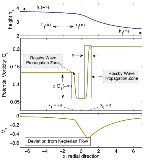
In order to anchor our intuition we begin this analysis by reconsidering the dynamics in a single-layer configuration. Under those conditions the shear is barotropic. The linearized equations we will need to solve are those given in the previous section with $\delta$ set to zero. With $\delta=0$ the upper layer has no dynamical effect upon the lower layer and, as such, the resulting dynamics describe flow of the lower layer entirely isolated from the upper layer. Therefore, the equations for the steady state are (17) with $\bar{Q}_{1}$ given and $\bar{v}_{1}$, as given in (19). For the linearized dynamics we solve only (32) with (28) to generate solutions for the lower layer perturbation enthalpy $\Pi_{1}^{\prime}$. We also assume the normal mode ansatz (33) and enforce that $\Pi_{1}^{\prime}(\pm L)=0$.

Figure (2) depicts the PV profile we shall examine here. We refer to it as the ‘double-tanh’ profile and is given by the form

$$\bar{Q}_{1} = A_{1}\left[1+\tanh\left(\frac{\Delta-x}{\xi}\right)\right]+$$ (35)

$$\hskip 56.9055ptB_{1}\left[1+\tanh\left(\frac{x-\Delta}{\xi}\right)\right]+C_{1},$$

where the constants are specified below. This functional form roughly represents a two-step PV-profile with the steps located at $x=\pm\Delta$ where $\Delta>0$ is some parameter. We will refer to twice this parameter as quantifying the width of this type of PV profile. The parameter $\xi$ represents the width of the transition in moving from one region of PV to the other. In the limit $\xi\rightarrow 0$ the transition from one region of PV to the other (e.g. near $x=\pm\Delta$ in Figure 2) is proportional to a Heaviside step function. One one hand we numerically we try to avoid the $\xi\rightarrow 0$ limit, yet on the other hand we want to have $\xi$ be small in order to relate the results of the model to our simplified understanding of the system. As such we typically choose $\xi=0.1$. Thus, as depicted in Figure 2, the limit $\xi\rightarrow 0$ makes the PV-profile look like two successive step functions or ‘defects’ in the PV. We interpret the length $2\Delta$ as quantifying the separation of these nominal defects of the PV.

We must now relate the constants $A_{1},B_{1},C_{1}$ to physically intuitive features of the model. Because we envisage a PV profile that has an induced velocity profile (as a deviation from the background Keplerian flow, i.e. $\bar{v}_{1}$) that is zero as $x\rightarrow\pm\infty$, inspection of (15) or (17) requires of us that

$$\lim_{x\rightarrow\pm\infty}\bar{Q}_{1}=\frac{2-q}{h_{1}(\pm\infty)}.$$ (36)

In other words, we design this profile to yield constant mean heights, $h_{1}(\pm\infty)$, in the limit of $x\rightarrow\pm\infty$. Of course, these heights may be different from one another but the constant asymptotic form of it ensures that the mean induced flow $\bar{v}_{1}$ correspondingly asymptotes to zero as $x\rightarrow\pm\infty$. As such this implies that

$$2A_{1}+C_{1} = \frac{2-q}{h_{1}(-\infty)},$$

$$2B_{1}+C_{1} = \frac{2-q}{h_{1}(\infty)}.$$

To complete this description we suppose that depth of the depression in $\bar{Q}_{1}$, located in the region $-\Delta<x<\Delta$, to be some factor $\phi>0$ of the asymptotic value of the PV as $x\rightarrow-\infty$, i.e. $\bar{Q}_{1}(-\infty)$. This amounts to

$$2A_{1}-C_{1}=\phi\bar{Q}_{1}(-\infty)=\phi\frac{2-q}{h_{1}(-\infty)}.$$

In summary, then, the barotropic model (35) is characterized by the five parameters: the asymptotic heights $h_{1}(\pm\infty)$, the symmetric positioning of the steps from $x=0$, $\Delta>0$, the relative depth of the PV-dip in the middle-zone of this model, $\phi$, and the width of the transition zones $\xi$. Note that the middle-zone has a width equal to $2\Delta$. The normal-mode system is additionally described by the shear parameter $q$.

A model similar to this one was considered in Umurhan (2010). Unlike here, however, the assumed PV-profile adopted in that previous study were (symmetric) step functions chosen to facilitate analytical tractability. In comparison to the model considered here, the step function used in Umurhan (2010) would correspond to the limit of this model in which $\xi\rightarrow 0$. Note also that the symmetry of the profiles studied in Umurhan (2010) is recovered here by choosing $h_{1}(\infty)=h_{1}(-\infty)$. We have therefore introduced the parameter $\xi$ to control the thickness of the transition from one zone to the next.

The rationale of introducing this feature into the model is to cleanly represent the propagation and interaction of Rossby waves without enduring the complexities of critical layers. Because Rossby waves represent disturbances that propagate in regions where the PV changes, setting $\xi$ to be small ensures that the waves are localized to those places where the PV changes the greatest. In this model, for example, there will be two Rossby waves, each of which are localized in $x$ at $x=\pm\Delta$ with a radial width of scale $\xi$. We typically use values of $\xi=0.1$ and this usually represented the Rossby wave dynamics without the appearance of critical layers. The robustness some solutions was evaluated by also generating solutions with values of $\xi=0.025$ (which necessitated using a higher resolution grid in order to resolve the transition zone with at least 5-7 grid points). Critical layers tended to appear for values of $\Delta\sim\xi$. However, we do not examine these situations in this study.

The barotropic incarnation of the Rossby wave instability was interpreted in Umurhan (2010) to arise as a result of the interaction of the two Rossby waves propagating along the azimuthal directions at the two locations, consistent with the more generic picture of interacting edgewave disturbances (Baines & Mitsudera 1994). An analogous form of this dynamic is present in this model and is especially pronounced for $\xi\ll 1$. For example, in reference to the PV profile shown in Figure 2, we observe that the jump in the PV is positive at the step located at $x=1$. Therefore, in the local frame of reference of the flow at $x=1$ and when taken in isolation, the supported Rossby wave propagates in the negative $y$ direction. Similarly, since the average change in the PV profile at $x=-1$ is negative, it can support a Rossby wave propagating in the positive $y$ direction when viewed from the local reference frame of the flow at $x=-1$. When the laboratory measured wavespeeds of both waves are nearly equal then instability may manifest itself, i.e. when the Hayashi-Young criterion is satisfied (Hayashi & Young 1987). Instability exists when the Rossby waves are essentially counterpropagating along the flow (Heifetz 1999) because it is only when the local propagating tendency of the Rossby wave is against the mean flow that the Hayashi-Young criteria of instability can be met.

In the next section we will also refer to an effective surface density. We define this here as

$$\Sigma_{1}(x)=\int_{0}^{h_{1}(x)}\rho_{1}dz=\rho_{1}h_{1}(x).$$ (37)

As can be seen $\Sigma_{1}$ is equivalent to $h_{1}$ in the single layer model, but will not be so in the two layer model. Henceforth we take $\rho_{1}=1$.

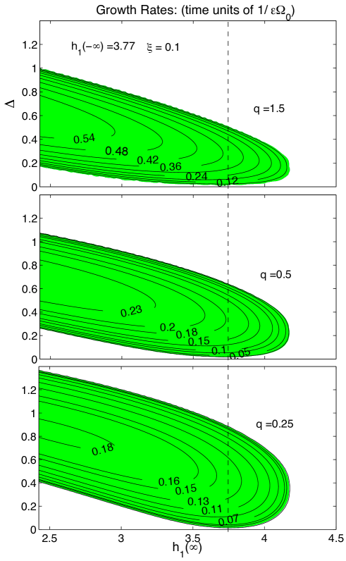
A representative summary of the results of this section is displayed in Figure 3. Even though we solve for the wavespeed $c$ we depict the growth rates Im$(-\omega)={\rm Im}(kc)$, together with having here (and henceforth) set $k=1$. The growth rates are quoted in time units used to derive the disk shallow water equations (see $\S 2$), namely, time is scaled in the longtime units $1/\epsilon\Omega_{0}$.

The results we plot here are an extension of the symmetric models considered in Umurhan (2010). Here we see that that the models do not have to display symmetric PV profiles in order for instability to surface and that, consistent with the results of Li et al. (2000), asymmetric PV profiles can just as easily lead to instability. We find that for a given set of layer parameters $h_{1}(\pm\infty)$ and $\phi$ (the depth of the PV depression) - as the background shear $q$ is lessened, the range of separation values $\Delta$ that admits instability is shifted toward larger values. In other words, weakening the shear means that profiles with steps further separated from one another will result in instability.

In terms of the picture of interacting Rossby waves, this is easily rationalized in the way outlined earlier in this section: (i) for instability to occur the laboratory measured phase speed of the Rossby waves along each step must be nearly the same, (ii) since the phase speeds of the Rossby waves are governed both by the background flow speed at the location of the step plus the intrinsic Rossby wave speed (as measured in the moving frame at the step) induced by the local change in PV at the transition region it follows that, (iii) with all else held equal, a reduction in the background shear requires the location of the defects at $x=\pm\Delta$ to be set further apart so that the laboratory measured phase speeds may be, once again, nearly equal.

When the step profiles are symmetric, i.e. when $h_{1}(-\infty)=h_{1}(\infty)$ instability may occur for separation $\Delta=0$ consistent with previous results in Umurhan 2010. However, as $h_{1}(\infty)$ begins to deviate away from the value $h_{1}(-\infty)$ then there exists a minimum value for the defect separation above which instability may occur. It is also interesting to note that there is a maximum disparity of heights beyond which there is no instability possible. E.g. for values of $h_{1}(\infty)>4.15$ with $q=1.5,\phi=0.1$ there is no instability possible in the model in Figure 3. The interpretation of this stability quality is once again similar to the above: varying $h_{1}(\infty)$ beyond some critical value results in individual waves whose speeds cannot possibly match each other. In particular, an increase of the speed of the wave at the step $x=\Delta$ occurs because increasing $h_{1}(\infty)$ means that the average PV-gradient increases at $x=\Delta$ step which, in turn, boosts the (in frame) counterpropagating Rossby wavespeed at the step.

The insensitivity of these results on $L$ has been verified. It is important to keep in mind that the growth rate values convergence to the values quoted once $L$ is greater than about 5. For values of $L<5$ the growth rates weaken. The presence of channel walls in problems like these creates the effect of ’image’ waves (like image charges in electrostatics problems, Drazin & Reid 1981) which act to inhibit phase locking. This behavior has been detailed in a study of the Rayleigh problem with variable wall positions (Heifetz et al. 2009) and the trend for instability suppression with more narrowly set walls is consistent with their findings.

The same character follows in the baroclinic cases studied except for one instance discussed later. Finally, consistent with the Howard Semicircle Theorem, we observe that as the shear is weakened the maximum value of the growth rate is reduced.

Figure 4: Baroclinic Jet profile model considered in this work.

Figure 5: Mixed barotropic-baroclinic results. The basic baroclinic model is examined for variations in $\Delta$ and $h_{0}(\infty)$. The pattern of regions of growth is similar to similar barotropic configurations. Note the particular absence of instability when $\Delta=0$.

5 Baroclinic profiles

In this section we solve the two layer problem. We assume that each layer has a single jump in PV but that their positions in $x$ are, in general, different from one another. We employ the basic type of model encountered in the previous section. In particular we suppose that the mean PV profiles

$$\bar{Q}_{0} = C_{0}+A_{0}\left[1-\tanh\left(\frac{x-x_{0}}{\xi}\right)\right],$$

$$\bar{Q}_{1} = C_{1}+A_{1}\left[1-\tanh\left(\frac{x-x_{1}}{\xi}\right)\right].$$ (38)

The steps for each layer are located at $x=x_{0},x_{1}$ respectively. Without loss of generality we place these positions symmetrically about the point $x=0$ and assign the position values $x_{0}=-\Delta$ and $x_{1}=\Delta$. $\Delta$ is a parameter as before, however, $\Delta$ can take on all values (and is not restricted to being strictly positive). As before, the thickness of the step in each layer is governed by the parameter $\xi$.

Figure 6: Baroclinic results depicting growth rates for varying values of the density ratio $\delta$ against the separation parameter $\Delta$. Shown are the growth rates for fixed values of $h_{0}(\pm\infty),h_{1}(\pm\infty)$ for Keplerian shear ($q=1.5$) and $\xi=0.05$. The range in separation values $\Delta$ in which instability occurs is reduced as $\delta$ is reduced. The growth rates are reduced as well. The implications are that interlayer interaction is weakened with a reduction of $\delta$.

Following the arguments laid out in the previous section, we require of the steady PV states to correspond to zero induced azimuthal flow $\bar{v}_{i}$ as $x\rightarrow\pm\infty$. Inspection of (14-15) indicates that the constants $A_{i},C_{i}$ must simultaneously satisfy

$$C_{0}+2A_{0}=\frac{2-q}{h_{0}(-\infty)-h_{1}(-\infty)},$$

$$C_{0}=\frac{2-q}{h_{0}(\infty)-h_{1}(\infty)}$$

$$C_{1}+2A_{1}=\frac{2-q}{h_{1}(-\infty)},\qquad C_{1}=\frac{2-q}{h_{1}(\infty)},$$

where the parameters $h_{i}(\pm\infty)$ are the asymptotic values of the layer heights in the appropriate limit of $x$. The only requirement we place upon the these are that $h_{0}(\infty)>h_{1}(\infty)$ and $h_{0}(-\infty)>h_{1}(-\infty)$.

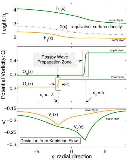
We solve for the steady configuration (16-19) using the above model for the PV profiles, which are governed by the six parameters $h_{i}(\pm\infty),\Delta,\xi$. The parameters of the steady configuration are also determined by the three remaining other parameters: the shear $q$, the density ratio $\delta$ and the domain size $L$. A qualitative example of the resulting states is shown in Figure 4. It is evident from the resulting flow that the mean deviation velocity fields are different from one another between layers indicating that the resulting flow state is baroclinic.

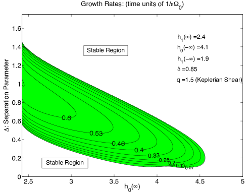
Figure 5 depicts the character typifying instability in these models. The parameters chosen here were meant to motivate maximum comparison to the results shown in the top graph of Figure 3. The top layer has a density ratio $\delta=0.85$ of the bottom layer. The results are qualitatively similar to the behavior of the barotropic model with certain modification to the region and degree of instability. Since, by design, there are only two waves which can interact - one emanating from the step in the upper layer and the other from the step in the lower layer - the interpretation of the instability is the same as for the barotropic case. Thus, baroclinic instability in this kind of baroclinic problem closely shadows the character of the instability in the barotropic case. The fundamental difference is, of course, the fact that the source of the Rossby waves are from different vertical layers.

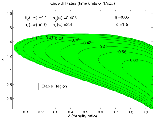
The coupling between layers is governed by the density contrast $\delta$. In Figure 6 we display how the growth rates are modified for a model in which we vary the separation $\Delta$ and the density contrast $\delta$. Indeed, as one might expect, both the occurrence of instability and its corresponding growth rate diminish as $\delta\rightarrow 0$. When viewed from the perspective of a normal mode problem, the lower layer essentially experiences no dynamical influence of the upper layer when the mass of the upper layer is vanishingly small (the lower layer “knows” of the upper layer due to the pressure fluctuations the upper layer induces upon the lower layer). From the mathematical viewpoint of a normal mode problem, both layers decouple from one another when $\delta=0$ (see the previous section). Nonetheless even for $\delta\approx 0$ the Rossby waves in each layer are finite (and non-zero) and propagate in isolation. Thus when $\delta$ is increased the bottom layer feels the upper layer in proportion to $\delta$ while the upper layer feels the bottom layer by the latter’s influence upon the upper layer’s thickness. We also note here that the figures show that growth rates persist as $\delta\rightarrow 1$ but we are less inclined to infer very much about this limit because as as $\delta\rightarrow 1$ the fundamental scaling relations leading to the Philips disk model begins to cause a break in the scaling assumptions behind the disk shallow water equations. Nevertheless the propensity for instability in these baroclinic models for $\delta$ not very close to zero suggests that baroclinic instability may be manifest in disks which are weakly stratified. We elaborate more upon this in Section 6.

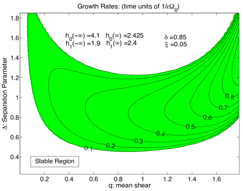
For a given set of model parameter values, varying the shear $q\rightarrow 0$ acts to reduce the growth rate of the instability and to push the unstable range of step separations $\Delta$ toward larger values. In Figure 7 we depict the growth rate trends for for variable values of $q$ and $\Delta$. Although the pattern of instability in this parameter diagram is more complex than the previous graphs, we see clearly that as the shear weakens (holding the separation fixed) the instability generally goes away. On the other end of the spectrum, as the Rayleigh limit is approached, i.e. $q\rightarrow 2$, the instability also appears to become suppressed. However we note here that the scaling ordering that is used to develop the disk shallow water equations begins to breakdown as $q$ approaches $2$ (see Umurhan 2008). We therefore consider these observed trends (in this particular limit) with more caution. A proper investigation of what happens in the Rayleigh limit should involve re-examining the equations of motion in that particular limit.

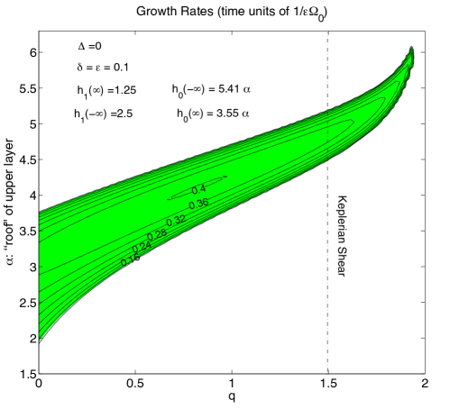
For given values of the shear $q$ there appears to be no parameter configuration that we could find in which there is both instability with the jets lying exactly on top of each other ($\Delta=0$) and where the instability does not vanish as $L\rightarrow\infty$. Such a configuration might correspond to a flow profile in which the jets model a baroclinically unstable setup relevant to more “traditional” baroclinic flow problems (like for the Earth and other Solar System planets). As we noted earlier, all of the results we report in this study are those in which the growth rates remain unaltered as the artificial domain walls in $x$ are made very large $L\gg 1$. In Figure 8 we show an example set of parameters in which there is instability but where the separation in $x$ of the two PV jumps is zero. The values of the top of the atmosphere $h_{0}(\pm\infty)$ are represented in a way such that the ratio of $h_{0}(\infty)/h_{0}(-\infty)$ remains fixed but the overall height of the atmosphere can vary with the parameter $\alpha$. For the example depicted, $h_{0}(\infty)=3.55\alpha$ and $h_{0}(-\infty)=5.44\alpha$. Thus $\alpha$ acts like a parameters varying the lid of the atmosphere. The values of the lower layer parameters $h_{1}(\pm\infty)$ are fixed. As such Figure 8 displays the growth rates as a function of $\alpha$ and $q$ with $L=10$. Instability appears to exist but for values of $\alpha$ so large that the atmosphere is effectively thin and tall. When we then increase the value of $L$ (holding fixed the remaining atmosphere parameters) the instability eventually vanishes.

We therefore conclude that the possibility of instability in a model in which the jets lie on top of each other, e.g. as implied by the results shown in Figure 8, is an artifact of the narrowness of the radial boundaries and is not likely to be possible for a real protoplanetary disk.

Figure 7: Baroclinic results depicting growth rates for varying values of the shear parameter $q$ against the separation parameter $\Delta$ with similar parameters found in the previous figure. As the shear tends to zero the values of $\Delta$ for instability increases. The growth rates also tend to zero. Growth rates become less reliable in the Rayleigh limit, $q\rightarrow 2$ (see text).

Figure 8: A model admitting baroclinic instability in which the jets in each layer lie exactly on top of each other ($\Delta=0$). The plot depicts the variation of the growth rates as a function of the shear $q$ and the so-called “lid” of the atmosphere $\alpha$ (see text). For this atmosphere model the radial boundaries are set at $L=10$. Keeping all parameters fixed but rerunning this atmosphere model with $L=15$ reveals that all of the instabilities depicted in this figure vanish.

6 Summary and Discussion

Baroclinic instability in the guise familiar in meteorology (in which isopycnals and isobars are misaligned) is feasible for cold protoplanetary disks, albeit in a mixed baroclinic-barotropic form owing to the strength of the underlying Keplerian shear. By using a two-layer Philips model we have further substantiated the conjecture made by Cabot (1984) and Knobloch & Spruit (1984,1985) that baroclinic instability is relevant for accretion disks. Aside from determining growth rates and interpreting the mechanics of the instability in terms of Rossby waves interacting across layers, it is also shown that the instability weakens in strength as the vertical density stratification of the layer is increased. The results of the two-layer model suggests that meteorological-type of baroclinic processes, which wholly depend on the mismatch of isobars and isopycnals in the mean state, is likely for disks that have weak vertical density stratification. Of course, this does not limit the full scope of possibilities and, as such, this must be analyzed more fully in the setting of more realistic disk models.

The use of the simple Philips two-layer model has been shown to be very good at capturing the essence of baroclinic flow dynamics present in continuously layered models of atmospheres (Vallis 2006). Comparison of growth rates determined for both the Eady Model (continuous vertical shear) and the Philips model shows that, although they are not precisely the same, the qualitative behaviors are consistent with one another and it is for this reason why the Philips model is so widely regarded as a useful theoretical platform to examine the physics of these and related processes. In fact, studies have been done in which multiple layer Philips models have been examined for the same problem yielding no significantly different results in classical meteorological investigations. This has partly to do with the geometry of the system being analyzed: in a planetary atmosphere there is usually a bottom boundary and the direction of gravity is the same.

By contrast we have investigated a disk model in which symmetry with respect to the disk midplane is imposed a priori. Thus the dynamics possible here, which allows only for a subset of possible phase relationships and Rossby wave interactions between the midplane layer and the layer above it, is a subset of a wider class of dynamical responses possible. For instance, if the restriction of midplane symmetry were relaxed then there comes into existence the possibility of new types of Rossby wave interactions independently involving three layers (the midplane and the two layers sandwiching the midplane) which will contain the dynamics of the two-layer system studied here. This may yield qualitatively new dynamical possibilities.

We should note here the similarities between traditional ‘meteorological’ baroclinic instabilities to other types of baroclinic processes investigated for both disks (e.g. Klahr & Bodenheimer 2003, Petersen et al. 2007a Petersen et al. 2007b, Lesur & Papaloizou 2010, Lyra & Klahr 2011) and the Sun (Gilman & Fox 1997, Zaqarashvili et al. 2010, to name only a few studies). In these analyses potential vorticity disturbances are effectively baroclinically torqued by some process that is either thermal or magnetic or, in some investigations, a combination of both. In those studies of magnetic Rossby waves in the Sun (e.g. Gilman & Fox 1997, Zaqarashvili et al. 2010) Rossby waves will propagate along those places where there are strong gradients in the solar differential rotation. Treated as a hydrodynamic problem, these Rossby waves are not necessarily unstable on their own, especially for differential rotation profiles inferred to be characteristic of the Sun’s tachochline. (Spiegel & Zahn 1992). However, when a strong toroidal field is added to the mix there appears an effective baroclinic source term (owing to the Lorentz force) which can render the wave unstable. In all of these studies the instabilities are global in character as is the instability investigated in this study since we have examined the fate of disturbances with azimuthal wavelengths on the scale of the disk.

The upcoming Paper III in this series examines an alternative derivation of the Shallow Water Equations for disks that lifts the restrictions placed upon the azimuthal scales as compared to the vertical and radial scales.

References

- (1) Baines, P. G., & Mitsudera, H. 1994, J. Fluid Mech., 276, 327
- (2) Balmforth, N. J., & Spiegel, E. A. 1996, Phys. D, 97, 1
- (3) Cabot, W. 1984, ApJ, 277, 806
- (4) Charney, J. G. 1947, J. Meteor., 4, 135
- (5) Drazin, P.G., & Reid, W.H. 1981 , Hydrodynamic Stability, Cambridge Univ. Press, Cambridge
- (6) Eady, E. T. 1949 Tellus, 1, 33
- (7) Fujimoto, M. Y. 1988 A&A, 198, 163
- (8) Gilman, P. A., & Fox, P.A. 1997 ApJ, 484, 439
- (9) Godon, P., & Livio, M. 1999, ApJ, 523, 350
- (10) Haine, T. W. N., & Marshall, J. 1998, J. Phys. Ocean., 28, 634
- (11) Hayashi, Y.-Y., & Young, W. R. 1987, J. Fluid Mech., 184, 477
- (12) Heifetz, E., Bishop, C. H., & Alpert, P. 1999 Q. J. R. Meteorol. Soc., 125, 2835
- (13) Heifetz, E., Harnik, N. & Tamarin, T. 2009 Q. J. R. Meteorol. Soc., 135, 2161
- (14) Hoskins, B. J., McIntyre, M. E., & Robertson, A. W. 1985 Q. J. R. Meteorol. Soc., 111, 877
- (15) Klahr, H. H., & Bodenheimer, P. 2003 ApJ, 582, 869
- (16) Knobloch, E., & Spruit, H. C. 1982 A&A, 113, 261
- (17) Knobloch, E., & Spruit, H. C. 1986 Geophys. Astrophys. Fluid Dyn., 32, 197
- (18) Knobloch, E., & Spruit, H. C. 1986 A&A, 166, 359
- (19) Lesur, G. & Papaloizou, J. C. B. 2010 A& A, 513, 60
- (20) Li, H., Finn, J. M., Lovelace, R. V. E., & Colgate, S. A. 2000 (LFLC-2000) ApJ, 533, 1023
- (21) Lyra, W. & Klahr, H. 2011 A&A, 527, 138
- (22) Meheut, H., Casse, F., Varniere, P., & Tagger, M. 2010 A&A, 516, A31
- (23) Molemaker, M. J., McWilliams, J. C., & Yavneh, I. 2005 J. Phys. Ocean., 35, 1505
- (24) Pedlosky, J. 1987, Geophysical Fluid Dynamics (2nd ed.), Springer-Verlag, New York
- (25) Petersen, M. R., Keith J., & Stewart, G. R. 2007a, ApJ 658 1236
- (26) Petersen, M. R., Keith J., & Stewart, G. R. 2007b, ApJ 658 1252
- (27) Phillips, N. A. 1954, Tellus,6, 273
- (28) Spiegel, E. A., & Zahn, J.-P. 1992, A&A 265, 106
- (29) Stone, P. H. 1970, J. Atm. Sci., 27, 721
- (30) Stone, P. H. 1971, J. Fluid Mech., 48, 659
- (31) Turner, N. J., Choukroun, M., Castillo-Rogez J., & Bryden G. 2012, Accepted ApJ arXiv:1110.4166v3[astro:ph]
- (32) Vallis, G. K. 2006, Atmospheric and Oceanic Fluid Dynamics, Cambridge University Press, New York
- (33) Umurhan, O. M. 2008, A&A, 489, 953
- (34) Umurhan, O. M. 2010, A&A, ,521, A25
- (35) Zaqarashvili, T. V., Carbonell, M., Oliver, R., & Ballester, J. L. 2010 ApJ, 709, 749