Thermomechanical properties of graphene: valence force field model approach

Abstract

Using the valence force field model of Perebeinos and Tersoff [Phys. Rev. B 79, 241409(R) (2009)], different energy modes of suspended graphene subjected to tensile or compressive strain are studied. By carrying out Monte Carlo simulations it is found that: i) only for small strains ($|\varepsilon|\lessapprox 0.02$) the total energy is symmetrical in the strain, while it behaves completely different beyond this threshold; ii) the important energy contributions in stretching experiments are stretching, angle bending, out-of-plane term and a term that provides repulsion against $\pi-\pi$ misalignment; iii) in compressing experiments the two latter terms increase rapidly and beyond the buckling transition stretching and bending energies are found to be constant; iv) from stretching-compressing simulations we calculated the Young modulus at room temperature 350$\pm 3.15$ N/m, which is in good agreement with experimental results (340$\pm 50$ N/m) and with ab-initio results [322-353] N/m; v) molar heat capacity is estimated to be 24.64 J/mol^-1K^-1 which is comparable with the Dulong-Petit value, i.e. 24.94 J/mol^-1K^-1 and is almost independent of the strain; vi) non-linear scaling properties are obtained from height-height correlations at finite temperature; vii) the used valence force field model results in a temperature independent bending modulus for graphene, and viii) the Gruneisen parameter is estimated to be 0.64.
Keywords : Thermomecahnical properties, Strain graphene sheet, Monte Carlo simulation, Molar heat capacity

I Introduction

Since the discovery of graphene in 2004, which is an almost two dimensional crystalline material, its exceptional mechanical properties have been studied Lee ; Giem2008 ; mayer ; fasolinonature ; arxiv2010 ; naturenanotechnology . Tensional strain in monolayer graphene affects its electronic structure. For example strains larger than $15\%$ changes graphene’s band structure and leads to the opening of an electronic gap naturephys . In recent experiments the buckling strain of a graphene sheet that was positioned on top of a substrate was found to be six orders of magnitude larger (i.e. $0.5-0.6\%$) than for graphene suspended in air arxiv2010 . Furthermore, some experiments showed that a compressed rectangular monolayer of graphene on a plastic beam with size 30$\times$100 $\mu m^{2}$ is buckled at about 0.7$\%$ strain compressionamall .

Elasticity theory for a thin continuum plate and the empirical interatomic potentials (EP) are two main theoretical approaches that have been used to study various mechanical properties measured in compressing and stretching experiments fasolinonature ; fasolino ; neekprb82 . Continuum elasticity theory does not give the atomistic features of graphene while the EPs, such as the Brenner potential (REBO) brenner ; brenner2002 and the LCBOPII potential LCBOP , can properly account for the mechanical properties of graphene. Despite the several benefits of these EPs, some special atomistic features of graphene subjected to compressive or tensile strains could not be explained. The different energy contributions in these potentials are mixed. For example, in REBO all the many body effects are put in the bond order term and the different important energy contributions are not separable.

It still remains unclear how large are the contributions of the different energy terms in strained graphene. Using the recently introduced valence force field (VFF) model by Perebeinos and Tersoff Tersoff2009 we show how the contribution of the different energy modes in strained graphene can be separated and we calculate their dependence on the value of strain.

The bending modulus of graphene at zero temperature was estimated using several interatomic potentials, e.g. the first version of the Brenner potential  brenner yields 0.83 eV, the second generation of the Brenner potential brenner2002 estimated it to be 0.69 eV, adding the third nearest neighbors (the dihedral angle effect) in the Brenner potential enhances it to 1.4 eV lu2009 , using the LCBOPII potential and continuum membrane theory the bending rigidity was found to be 0.82 eV fasolinonature ; LCBOP , Tersoff’s VFF model estimated it to be 2.1 eV, and from ab-initio energy calculations it was found to be 1.5 eV Yakobson (note that ‘bending rigidity’ (‘bending modulus’) is used for a membrane stiffness (an atomistic sheet)). Despite these studies the temperature dependence of the bending modulus is poorly known. An increasing behavior versus temperature for the bending rigidity was found  fasolinonature by using Monte Carlo simulations with the LCBOPII potential and membrane theory concepts. In contrast, Liu et al liuAPL found a decreasing bending rigidity with temperature using the REBO. Here we show that the VFF model predicts a temperature independent bending modulus.

In this study we employ VFF and carry out standard Monte Carlo simulations in order to calculate and compare the different energy modes of a graphene sheet that is subject to axial strains. The total energy is found to be different for compressing and stretching when strains are applied larger than $|2|\%$. Two important terms, i.e. stretching and bending, vary differently depending on the way that one stretches or compresses the system. We find that out-of-plane and $\pi-\pi$ terms have much larger contributions in compression experiments when compared to stretching. Furthermore, we used this potential to calculate Young’s modulus at room temperature from stretching-compressing simulations. We also calculate the molar heat capacity. Our Monte Carlo simulations show that the VFF potential yields a temperature independent bending modulus.

This paper is organized as follows. Section II contains the essentials of the VFF model for graphene. The simulation method for strained graphene will be presented in Sec. III. Different energy modes of strained graphene are studied in Sec. IV. In Sec. V the molar heat capacity for non-strained suspended graphene is calculated. Temperature effects of the bending modulus of graphene with periodic boundary condition are presented in Sec. VI and the scaling properties of graphene at finite temperature are investigated in Sec VII. We will conclude the paper in Sec. VIII.

II Elastic energy of graphene

There are two main classical approaches for the investigation of the elastic energy of graphene: 1) the continuum approach based on elasticity theory, and 2) the atomistic description using accurate interatomic potentials.

The total energy of a deformed membrane consists of two important terms: stretching and bending. For almost flat and continuum membrane using Monge representation the surface area element $dA$ can be approximated by a flat sheet area element in the x-y-plane, i.e. $dA\approx dxdy$ and the bending energy is written as $\frac{1}{2}\int dxdy\kappa(\nabla^{2}h)^{2}$ where $\kappa$ is the bending rigidity and $h$ is the out-of-plane deformation of the membrane at point $(x,y)$. The stretching term for an isotropic continuum material in the linear regime includes two independent parameters: the shear modulus ($\mu$) and the Lamé coefficient ($\lambda$) and is written as $\frac{1}{2}\int dxdy[2\mu u^{2}_{\alpha\beta}+\lambda u_{\alpha\alpha}^{2}]$. Here $u_{\alpha\beta}=\frac{1}{2}[\partial_{\alpha}u_{\beta}+\partial_{\beta}u_{\alpha}+\partial_{\alpha}h\partial_{\beta}h]$ is the second rank symmetric tensor with $\alpha,\beta=1,2$ and $u_{\alpha}(x,y)$ is the $\alpha^{th}$ component of the displacement vector. Neglecting the last term in the strain tensor makes the stretching term linear and decouples the bending and stretching energy. Therefore for an isotropic and continuum material for small deformations and with the assumption of a nearly flat membrane ($|\nabla h|^{2}\ll 1$) the strain energy ($U_{T}$) can be written as [18]

$$U_{T}=\frac{1}{2}\int dxdy[\kappa(\nabla^{2}h)^{2}+2\mu u^{2}_{\alpha\beta}+\lambda u_{\alpha\alpha}^{2}].$$ (1)

The integral is taken over the projected area of the membrane into the x-y-plane. For isotropic materials and in the linear approximation the mentioned parameters are related to the Young modulus ($Y$) and Poisson’s ratio ($\nu$) as $\mu=Y/(2(1+\nu))$ and $\lambda=2\mu\nu/(1-2\nu)$. Equation (1) can be rewritten in terms of the Fourier components of $h$ and yields the scaling properties of the sheet. Despite these benefits, this continuum model does not include self-avoidance, the natural condition of true physical systems and does not show atomistic details of the membrane under different boundary conditions. All these deficiencies originate from the continuity assumption. Assuming graphene as a continuum plate limits the study to only bending and stretching modes.

Due to the hexagonal symmetry of the flat monolayer graphene lattice, it is elastically isotropic which implies that the the bending modulus is independent of the direction at least within the linear elastic regime lu2009 . However, the graphene monolayer can exhibits anisotropic behavior in the nonlinear regime where distortions are no longer infinitesimal. The larger stretches, the stronger anisotropy and non-linearity effects. Cadelano et al found that monolayer graphene is isotropic in the linear regime, while it is anisotropic when nonlinear features are taken into account poisson .

The recently introduced VFF model in Ref. Tersoff2009 is expected to be able to describe both compression and stretching experiments by separating the contribution of the various energy modes. This model includes explicitly the various relevant energy terms which describe the change in the bond lengths, bond angles and torsional effects. The total energy density is written as

$$E_{T}=\frac{1}{NS_{0}}(E_{st}+E_{be}+E_{out}+E_{bo}+E_{p}+E_{co}),$$ (2)

where $N$ is the number of atoms and $S_{0}=\frac{3\sqrt{3}}{4}a_{0}^{2}$ is the surface area of the unit cell of the honeycomb lattice. In the following we will discuss the different terms in Eq. (2). Note that the energy reference is set to zero. Assuming $a_{0}=1.42\,\AA$ as the unit of length, the ‘stretching’ and ‘bending’ (bending of the bond angle) terms are

$$E_{st} = \frac{1}{2}K_{s}\sum_{i,j}(\delta r_{ij})^{2}$$ (3)

$$E_{be} = K_{be}\sum_{i,j<k}(\cos(\theta_{ijk})-\cos(\theta_{0}))^{2}$$ (4)

where $\delta r_{ij}=r_{ij}-1$ and $\theta_{0}=2\pi/3$. In Eqs. (3) and (4) $r_{ij}$ is the bond length between atom ‘i’ and ‘j’, $\theta_{ijk}$ is the angle between the nearest neighbor atoms ‘i’, ‘j’ and ‘k’ and $\theta_{0}$ is the equilibrium angle between three nearest neighbor atoms. $E_{st}$ is the two-body stretching term responsible for bond stretching. $E_{be}$ is the bending energy due to the bond angles. Here, all bond angles will be considered. The above two terms results in a quasi-harmonic model LCBOP . Later, we will find that these two terms become constant as function of strain when beyond the buckling point in a compression experiment.

The stiffness against ‘out-of-plane’ vibration is provided by

$$E_{out}=K_{out}\sum_{i,j<k<l}(\frac{3\overrightarrow{r_{ij}}\cdot\overrightarrow{r_{ik}}\times\overrightarrow{r_{il}}}{r_{ij}r_{ik}+r_{ij}r_{il}+r_{ik}r_{il}})^{2},$$ (5)

where the summation is taken over the first neighbors of atoms $`i$’ and taking care of not double counting. In Eq. (5) $\overrightarrow{r_{ij}}$ is the distance vector between atom ‘i’ and ‘j’. Hence there are three different terms for each atom. Correlations between bond lengths are provided by the ’bond order’ term

$$E_{bo}=K_{bo}\sum_{i,j<k}\delta r_{ij}\delta r_{ik},$$ (6)

where for each bond length with central atom ‘i’ three different terms are considered.

The misalignment of the neighboring $\pi$ orbital is given by the ‘$\pi-\pi$’ term

$$E_{p}=\frac{1}{2}K_{p}\sum_{i,j}|\overrightarrow{\pi_{i}}\times\overrightarrow{\pi_{j}}|^{2},$$ (7)

where

$$\overrightarrow{\pi_{i}}=3\frac{\overrightarrow{n_{ijk}}+\overrightarrow{n_{ikl}}+\overrightarrow{n_{ilj}}}{r_{ij}r_{ik}+r_{ij}r_{il}+r_{ik}r_{il}}.$$ (8)

$\overrightarrow{n_{ijk}}=\overrightarrow{r_{ij}}\times\overrightarrow{r_{ik}}$ is a vector normal to the plane passing through the vectors $\overrightarrow{r_{ij}}$ and $\overrightarrow{r_{ik}}$. This kind of interaction plays an important role in the interlayer interaction in graphitic structures. Note that the simple two body interaction gives only $2\%$ of the local density of state (LDA) result for the energy difference between AA and AB stacked graphite prb2005 .

The last term takes into account the coupling between bond stretching and bond angle bending (bond length-bond angle cross coupling), i.e. the ‘correlation’ term

$$E_{cor}=K_{cor}\sum_{i,j<k}\delta r_{ij}(\cos(\theta_{ijk})-\cos(\theta_{0})).$$ (9)

The coefficients in the above equations ($K_{s},K_{be}$ and so on) were recently parameterized by Perebeinos and Tersoff Tersoff2009 such that the phonon dispersion of graphene was accurately described. These parameters are listed in Table I.

Table 1: Parameters of the energy model (Eq. (2)) are taken from Ref. Tersoff2009 . Units are in eV.

$K_{s}$	$K_{be}$	$K_{out}$	$K_{bo}$	$K_{p}$	$K_{cor}$
37.04	4.087	1.313	4.004	0.016102	4.581

Table 2: Young’s modulus of graphene in units of N/m.

Experimental		Classical (T=300 K)				Ab-initio (T=0 K)			Tight-Binding
340$\pm$50	350$\pm$3.15	355$\pm$21	384	345$\pm$6.9	336	352.54	351.75	322	312
Ref. Lee	Present∗	Ref. fasolino b	Ref.  TersoffBrenner c	Ref. Yakobson	Ref. Ortwin	Ref. diamond	Ref. Liu	Ref. Jphys	Ref. poisson

^∗ VFF model Tersoff2009 , ^b LCBOPII potential, ^c Tersoff-Brenner potential .

III Simulation method: strained graphene

In order to compress (stretch) graphene nanoribbons, we have carried out several standard Monte Carlo simulations fasolinonature of a suspended graphene sheet at finite temperature. Equation (2) is used to calculate the total energy of the system. Our sample is a rectangular graphene sheet with $l_{x}\times l_{y}$ dimensions in $x$- and $y$-directions, respectively, containing $N_{0}$=1600 atoms. The sheet is strained along the armchair or the zig-zag direction. Strain is always applied along $x$. When graphene is strained along the armchair direction we named it armchair graphene -AC- ($l_{x}$=85.2 Å, $l_{y}$=49.19 Å) and strained graphene along zig-zag direction is named zig-zag graphene-ZZ- ($l_{x}$=98.38 Å, $l_{y}$=42.6 Å). Periodic boundary conditions are applied along the lateral direction i.e. zigzag direction in AC graphene and along the armchair direction for ZZ graphene. Our simulation starts with a flat sheet, and we allow then the system to thermally equilibrate such that the total energy no longer changes. Temperature is typically taken $T$=300 K, except when otherwise indicated. Figure 1(a) shows a snap shot of the relaxed unstrained ZZ graphene at $T$=300 K (note that the supported ends are fixed). We found that the graphene sheet is corrugated after relaxation which are the intrinsic thermal ripples in graphene. Thus the used VFF is able to display true structural properties. These ripples are vital in order to make suspended graphene stable and are therefore crucial for the stability of a flat 2D crystal at finite temperature fasolinonature .

To simulate a suspended sheet we fixed two atomic rows at both longitudinal ends. These boundary atoms are not included in the summations when calculating the different energy contributions (in Eqs. (2-9)), i.e. $N=N_{0}-40$. We compress/stretch the system with a slow rate, i.e. in every million Monte Carlo steps the longitudinal ends are reduced/elongated with about $\delta=$0.02 Å  such that the system stays in thermal equilibrium. After obtaining the total desired strain $\varepsilon$, we wait for an extra 4 million steps during which the system can relax. For example, a strain (applied in $x$-direction) of $\varepsilon=1.2\%$ is achieved after 29$\times 10^{6}$ Monte Carlo steps.

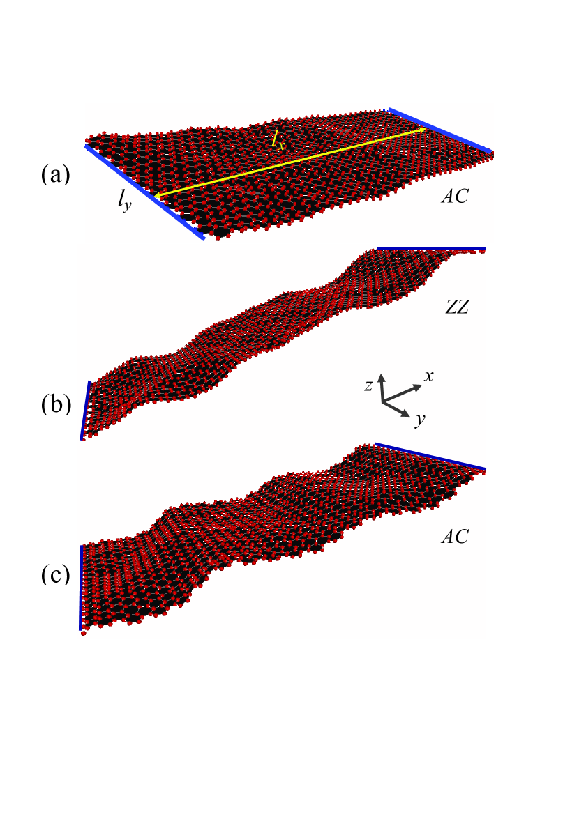
Figure 1: (Color online) Snap shot of a suspended graphene sheet at $T$=300 K using the valence force model (Eq. (2)). Blue lines indicate the position of fixed atoms in $x-y$ plane. (a) Unstrained, (b) compressed ZZ graphene, and (c) compressed AC graphene.

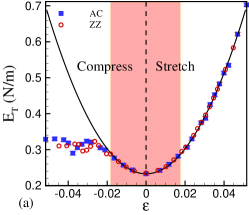
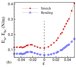
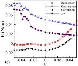
Figure 2: (Color online) (a) Total energy of a graphene sheet subjected to stretching and compression for AC and ZZ. (b) Contribution of the bending (Eq. (4)) and the stretching (Eq. (3)) terms of the total energy for AC. (c) Contribution of the other remaining terms given by Eqs. (5)-(9) for AC.

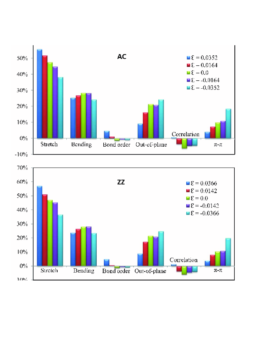
Figure 3: (Color online) Contribution of the different energy terms to the total energy for three typical values of the strain in AC (Top) and ZZ (Bottom) graphene.

IV Different energy modes for strained graphene

Figures 1(b,c) show two snap shots of compressed ZZ and AC graphene, respectively when $\varepsilon$=-2$\%$. It is interesting that the rippled structure is different in the two cases. This is due to the different out-of-plane and $\pi-\pi$ interaction terms around and beyond the buckling transition points, i.e. $\varepsilon\lesssim-2.5\%$.

The variation of height, $\widetilde{\Delta h}=\sqrt{<h^{2}>-<h>^{2}}$, in Fig. 1(a) after 10 million MC steps fluctuates around 0.2 Å which is comparable with those found when using REBO EURoJB . In Figs. 1(b,c) for compressed nanoribbons of about $\varepsilon$ = -2.0 $\%$ $\widetilde{\Delta h}$ is 0.5 Å  after 54 million MC steps. The larger compressive strain yields a larger height variance.

Figure 2(a) shows the variation of the total energy (Eq. (2)) with applied strain at $T$=300 K. The vertical dashed line separates compressive (left) and tensile strain (right). Square (circular) symbols refer to AC (ZZ) graphene. Notice that AC and ZZ strained graphene result in the same energy, although their ripples structure (see Figs. 1(b,c)) can be rather different. Note that the energy curve is no longer symmetric around $\varepsilon=0$ beyond the colored rectangle where $|\varepsilon|\gtrsim 0.02$. Inside this region the deformation is symmetric and the harmonic approximation to the total energy works well as shown by the full black (parabolic) curve in Fig. 2(a). The solid curve is a quadratic fit according to $E_{T}=E_{0}+\frac{1}{2}Y\varepsilon^{2}$ for only positive strains, where the fitting parameter $Y$ is Young’s modulus and $E_{0}$ is the energy of the graphene sheet in the absence of strain. We found $E_{0}$=0.232$\pm$0.002 N/m and $Y$=350.42$\pm$3.15 N/m for room temperature. The calculated error bars are derived from the fitting procedure of our numerical data. The best fit yielded the smallest deviation from the harmonic behavior. Our result for the room temperature Young’s modulus is close to the experimental value (340$\pm 50$ N/m) and is within the ab-initio results (335-353 N/m) and is in agreement with those obtained from other classical force fields such as (LCBOPII fasolino and Tersoff-Brenner TersoffBrenner ) and Tight-Binding poisson , see Table. II. Note that Perebeinos and Tersoff estimated $Y$ at zero temperature and found 1.024 N/$m^{2}$ (343.04 N/m)  Tersoff2009 . Here we calculated $Y$ at room temperature via stretching-compression simulations. Different force fields are parameterized such that they describe a set of chosen experimental data of particular experimental effects. For example, the VFF model can not be used to study hydrogenation, melting and defect formation in either graphene or carbon nanotubes sheets, while the REBO has been set-up such that it can be used in those cases. The property that the energy can be separated into different energy modes and the simplicity of coding the VFF potential are two important advantages of this model.

Notice that the total energy for AC (square symbols in Fig. 2(a)) and ZZ (circular symbols in Fig. 2(a)) graphene are almost the same which is in agreement with the results of Ref. poisson . Graphene acts isotropically in the linear elastic limit. Beyond the harmonic regime there is a small local maximum in the energy for compression which is related to the buckling of graphene. Notice that in this regime there are small differences between ZZ and AC sheets. The buckling threshold is about $\varepsilon_{b}\simeq-2.5\%$. The buckling strains is smaller than those found by using REBO neekprb82 , i.e. -0.86$\%$. Notice that both the boundary conditions and the employed interatomic potentials are responsible for the difference in the buckling thresholds. The main difference is due to the different potential. The VFF model is not a bond-order potential (REBO). As we mentioned in the introduction the bending modulus predicted by REBO is about 0.69-0.83 eV which is smaller than the one predicted by the VFF model (2.1 eV). Therefore, we expect a larger buckling transition using REBO and a smaller one using VFF model (considering the negative sign for compressive strains). Another important reason for the different result is the calculations method. Here we used Monte Carlo (time is meaningless) and in Ref. [9] we used Molecular dynamics simulations.

Figure 2(b) shows the contribution of the two important energy terms, i.e. stretching and bending as given by Eq. (3) and Eq. (4), respectively, for strained AC graphene. Notice that the stretching energy is larger than the bending and that the rate of increase for stretching is different. In the compression part (i.e the region to the left of the vertical dashed line), after the buckling points these energies are almost constant. Thus increasing compression beyond the buckling point does not change the bending and stretching energies. Figure 3 shows the contribution of the different energy terms (scaled by $E_{T}$) for three values of the strain for both AC and ZZ graphene (e.g. the first set of bars to the left refer to $100\times E_{st}/E_{T}$ for each particular strain shown in the legends). From Fig. 3, we conclude that the contribution of the energy terms (Eq. (4) and Eq. (7)) which are not determinable in the continuum elasticity energy approach (Eq. (1)) are substantial and should be retained when describing strained graphene at the atomistic scales

Figure 2(c) shows the variation of the other terms in the energy, Eqs. (5-9), with strain. The energy for $\pi$-$\pi$ repulsion and out-of-plane increase (decrease) with compression (stretching) and they behave opposite to the other terms. In compression experiments the sheets become strongly corrugated and neighbor $\pi$ orbitals become more misaligned. In other words the normal to the adjacent surfaces, e.g. - $\overrightarrow{n_{ijk}}$- and -$\overrightarrow{n_{ijl}}$- become more misaligned which results in an increase of the total energy. Notice also that the bond order term is smaller and negative in the compression part with respect to the stretching part. The correlation between the bond lengths is always negative for the compression part. We found that the relative contribution of the different energy modes for stretching and compression of AC and ZZ graphene are almost the same, compare Fig. 3(a) and Fig. 3(b). However as we see from Figs. 1(b,c) the structure of the ripples depends on the direction of the applied strain. In the case of AC the ripples are regular (sinusoidal shape) while they exhibit an irregular pattern in ZZ graphene. Note that the buckling in plates is generally known to depend on the plate geometric parameters book ; neekprb82 . Notice that, the dependence of the ripple structure of the graphene sheets on the sheet geometry has been demonstrated experimentally in Ref. arxiv2010 .

V Molar heat capacity

Next, we simulated graphene at different temperatures. Figure 4(a) shows the temperature dependence of the average total energy and of the six energy terms for $\varepsilon=0$. Notice that all energy terms vary linearly with $T$. The quantity $C_{V}=N_{A}S_{0}\frac{d\langle E_{T}\rangle}{dT}$ gives the potential energy contribution to the molar heat capacity of the system at constant volume, where $N_{A}$ is Avogadro’s constant. Note that we first relaxed the volume of the system by performing a constant pressure-temperature (NPT) Monte Carlo simulation (which removes possible boundary strains). Then we fixed the boundaries to the found relaxed size and allowed for additional thermal relaxation (i.e. constant volume-temperature Monte Carlo simulation or NVT). During this new thermal relaxation no strain is applied $\varepsilon=0$, thus, the calculated heat capacity corresponds to constant volume molar heat capacity. Surprisingly, we found that $C_{V}=12.33$ J mol^-1 K^-1 which is almost half of the Dulong-Petit value, i.e. $3\Re$=24.94 J mol^-1 K^-1. Notice that $\langle E_{T}\rangle$ is the average of the potential energy of graphene which is taken over 4 million Monte Carlo steps. Assuming that the average of the kinetic term equals the average potential energy ($\langle E_{T}\rangle$) according to the equipartition theorem (in the harmonic regime), we can write the total energy $\langle E\rangle=\langle E_{T}\rangle+\langle K\rangle=2\langle E_{T}\rangle$ and then the total heat capacity is found to be $24.66\pm$0.10 J mol^-1 K^-1. The obtained result is close to our previous result obtained using REBO, i.e. 24.98$\pm$0.14 J mol^-1 K^-1 neek-amalPRB2001 . In Ref.  fasolino the heat capacity at 300 K was found to be 24.2 J mol^-1 K^-1. We have performed many simulations at different temperatures for strained graphene and found always a linear $\langle E_{T}\rangle-T$ curves. Fig. 4(b) shows the variation of $C_{V}$ versus strain. It is interesting to note that $C_{V}$ is slightly lower ($\thicksim 1.0\%$) in compressed graphene as compared to stretched graphene.
Furthermore, we performed several simulations using the same sample employing the AIREBO potential AIREBO within LAMMPS software lammps . It is interesting to know that AIREBO gives (in the range of 10 K-1000 K) $C_{V}$=24.92 J mol^-1 K^-1 which was found to be independent of temperature. Therefore, the VFF model, REBO and AIREBO predicts temperature independent heat capacity.
On the other hand we found that the VFF model, REBO and AIREBO, give a linear increase in the carbon-carbon bond length ($a$) with temperature. The resulting bond length thermal expansion coefficients for the VFF model, REBO and AIREBO are $\alpha=\frac{1}{a_{0}}\frac{da}{dT}=(5.0\pm 0.07)\times 10^{-6}K^{-1}$, $(5.0\pm 0.03)\times 10^{-6}K^{-1}$ and $(7.0\pm 0.04)\times 10^{-6}K^{-1}$ respectively. The Gruneisen parameter is defined as $\gamma=\frac{\alpha B}{C_{V}\rho}$ where B is the two dimensional bulk modulus for graphene, i.e $B=12.7$ eVÅ^-2 fasolino , and $\rho$ is the mass density of graphene, i.e. $\rho=12.0/S_{0}=7.6\times 10^{-4}$g m^-2. Using our result for $C_{V}$ and $\alpha$ gives $\gamma=0.64$ which is better estimation for the Grüneisen parameter than the one found in Ref. Tersoff2009 , i.e. -0.2, and is closer to the experimental result, i.e. 2.0 Gruneisen .

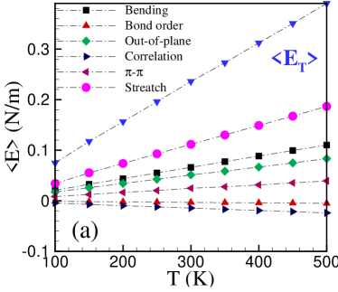
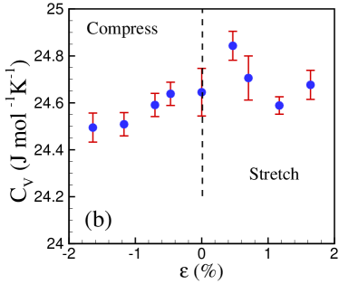
Figure 4: (Color online) (a) Temperature dependence of the various energy modes of a suspended graphene sheet which is suspended along arm-chair direction. (b) Variation of molar heat capacity at constant volume for graphene subjected to compressive and tensile strains.

Figure 5: (Color online) Temperature dependence of the bending modulus of graphene (a) and variation of the nanotube curvature versus nanotube index, i.e $m$.

VI Temperature effect of the bending modulus

A common method for calculating the bending modulus of graphene is by performing several simulations as function of the radius ($R$) of the curved tubes and extrapolates the results to $R\rightarrow\infty$ (see Fig. 5(b)). Hence, one can calculate the elastic energy of carbon nanotubes as a function of the inverse square of the radius, $E=\frac{1}{2}\kappa R^{-2}$. The coefficient $\kappa$ in the elastic energy gives the bending modulus of graphene. In order to study the effect of temperature on the bending modulus of graphene we have carried out several NPT Monte Carlo simulations (constant pressure with periodic boundary condition) at different temperatures. For each particular temperature we have 8 different tubes. In this part of the paper, our systems are different armchair carbon nanotubes with radius $R=3\,m^{2}\,a_{0}/2\pi$ and initial length 10 nm. We used eight armchair carbon nanotubes with index (m,m) for m=5,10,15,20,25,30,35,40. For each particular nanotube with index $m$, we carried out several NPT Monte Carlo simulations with periodic boundary condition along the nanotube axis and varying temperatures in the range 10 to 1000 K. Calculating $E_{T}$ by using Eq. (2) for all nanotubes at temperature $T$, we fitted $\frac{1}{2}\kappa R^{-2}$ to the data and found the bending modulus (stiffness), $\kappa$, at $T$. From Fig. 5(a) we notice that $\kappa$ is practically temperature independent and is about 2.02 eV. Thus the present VFF model results in a temperature independent bending modulus. Using membrane theory to calculate the bending rigidity of graphene shows that different potentials leads to conflicting temperature dependence for the bending rigidity, e.g. LCBOPII  fasolinonature yields an increase of the bending rigidity with temperature while REBO predicts a decreasing dependence liuAPL .

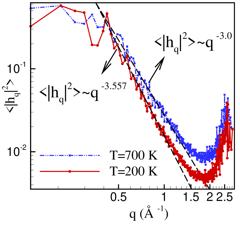
Figure 6: (Color online) The absolute value of the square of the Fourier transform of atomic heights of C-atoms ($|h_{q}|^{2}$) versus the absolute value of the wave vectors of the graphene lattice.

VII Scaling properties

In the harmonic regime the power spectrum of the graphene solid membrane can be obtained by calculating $<|h_{q}|^{2}>$ where $h_{q}$ is the Fourier transform of the height of the atoms ($h$) and $q$ is the norm of the wave vector $\overrightarrow{q}$ $(=(q_{x},q_{y})=2\pi(\frac{n_{x}}{l_{x}},\frac{n_{y}}{l_{y}}))$ with integers $n_{x}$ and $n_{y}$ where $l_{x}$ and $l_{y}$ are the longitudinal and lateral size of the graphene sample. It is important to note that in this section we simulated a graphene sheet with initial size $l_{x}=230.04\,\AA$  and $l_{y}=221.35\,\AA$ ($N$=19440) using standard NPT Monte Carlo simulations with periodic boundary conditions in both directions (the method is similar to that reported in Refs. [4,10]). We estimated the spectral modes $h_{q}$ by fitting $|h_{q}|^{2}$ to a $q^{\alpha}$ function, from which we extract the power law $\alpha$. Figure 6 shows the variation of $|h_{q}|^{2}$ (averaged over 500 Monte Carlo realizations where 5 neighboring points were accumulated and averaged to a single point in order to make the curves smoother) versus $q$ for graphene at two temperatures 200 K and 700 K. The dashed lines are power law fits. Notice that $\alpha\neq-4$ which clearly indicates that anharmonic effects are present in the used VFF potential. Moreover we see that $\alpha$ decreases with decreasing temperature ($\alpha=$-3.0 for T=700 K and $\alpha=$-3.557 for T=200 K) which hints that a more harmonic behavior is found at low temperature when using the VFF potential. The latter temperature dependence is in agreement with the REBO predictions EURoJB . Notice that the REBO is a bond-order interatomic potential. Note that the peaks in Fig. 6 are related to first Bragg-peak, $4\pi/3a_{0}=2.94\AA$  due to the discreteness of the graphene lattice. Notice that the modulation amplitude in Fig. 6 for T=200 K is about 0.5Å and for T=700 K is about 0.7Å  which are temperature and size dependent quantities, the larger the size the larger the amplitudes (here graphene has dimension $221\times 230$ Ų). Here, we did not study the effect of size and refer the reader to Refs. fasolinonature ; fasolino where such a study can be found.

VIII Conclusions

In this study, we showed that the recently proposed valence force field model (VFF) Tersoff2009 for graphene enables to compare the contribution of the different energy terms when straining graphene. In a stretching experiment the main energy contributions are due to stretching and bending terms while for compressive strains also other terms such as out-of-plane and $\pi-\pi$ interaction terms play an important role. We found that using such a classical approach gives accurate values for the Young’s modulus at room temperature which are found to be as accurate as those using ab-initio methods. The calculated Young’s modulus is close to the experimental result. The total energy is quadratic in $\varepsilon$ for strains smaller than $|2\%|$. The current VFF model predicts a temperature independence bending modulus. The temperature dependence of the total strain energy yields an acceptable value for the molar heat capacity of graphene which is too a large extend independent of the applied strain. The Gruneisen parameter is found to be positive and about 0.64.

Acknowledgment. We acknowledge helpful comments by V. Perebeinos, S. Costamagna, A. Fasolino and J. H. Los. This work was supported by the Flemish science foundation (FWO-Vl) and the Belgium Science Policy (IAP).

References

- (1) C. Lee, X. Wei, J. W. Kysar, and J. Hone, Science 321, 385 (2008).
- (2) T. J. Booth, P. Blake, R. R. Nair, D. Jiang, E. W. Hill, U. Bangert, A. Bleloch, M. I Gass, K. S. Novoselov, M. I. Katsnelson, and A. K. Geim, Nano. Lett. 8, 2442 (2008).
- (3) J. C. Meyer, A. K. Geim, M. I. Katsnelson, K. S. Novoselov, T. J. Booth, and S. Roth, Nature (London) 446, 60 (2007).
- (4) A. Fasolino, J. H. Los, and M. I. Katsnelson, Nature Materials 6, 858 (2007).
- (5) O. Frank, G. Tsoukleri, J. Parthenios, K. Papagelis, I. Riaz, R. Jalil, K. S. Novoselov, and C. Galiotis, ACS-Nano 4, 3131 (2010).
- (6) W. Bao, F. Miao, Z. Chen, H. Zhang, W. Jang, C. Dames, and C. Ning Lau, Nat. Nanotech. 4, 562 (2009).
- (7) F. Guinea, M. I. Katsnelson, and A. K. Geim, Nat. Phys. 6, 30 (2009).
- (8) G. Tsoukleri, J. Parthenios, K. Papagelis, R. Jalil, A. C. Ferrari, A. K. Geim, K. S. Novoselov, and C. Galiotis, Small 5, 2397 (2009).
- (9) M. Neek-Amal and F. M. Peeters, Phys. Rev. B 82, 085432 (2010).
- (10) K. V. Zakharchenko, M. I. Katsnelson, and A. Fasolino, Phys. Rev. Lett. 102, 046808 (2009).
- (11) D. W. Brenner, Phys. Rev. B 42, 9458 (1990).
- (12) D. W. Brenner, O. A. Shenderova, J. A. Harrison, S. J. Stuart, B. Ni, and S. B. Sinnot, J. Phys.: Condens. Matter 14, 783 (2002).
- (13) J. H. Los, L. M. Ghiringhelli, E. J. Meijer, and A. Fasolino, Phys. Rev. B 72, 214102 (2005).
- (14) V. Perebeinos and J. Tersoff, Phys. Rev. B 79, 241409(R) (2009).
- (15) Q. Lu, M. Arroyo, and R. Huang, J. Phys. D: Appl. Phys. 42 102002 (2009).
- (16) K. N. Kudin, E. Scuseria, and B. I. Yakobson, Phys. Rev. B 64, 235406 (2001).
- (17) P. Liu and Y. W. Zhang, Appl. Phys. Lett. 94, 231912 (2009).
- (18) K. Zakharchenko, PhD Thesis, Radboud University Nijmegen, The Netherlands ‘Temperature effects on graphene: from flat crystal to 3D liquid’ (2011).
- (19) E. Cadelano, P. L. Palla, S. Giordano, and L. Colombo, Phys. Rev. Lett. 102, 235502 (2009).
- (20) A. N. Kolmogorov and V. H. Crespi, Phys. Rev. B 71, 235415 (2005).
- (21) X. Chang, Y. Ge, and J.M. Donga, Eur. Phys. J. B 78, 103 (2010).
- (22) K. H. Michel and B. Verberck, Phys. Stat. Sol. (b) 245 2177 (2008).
- (23) O. Leenaerts, H. Peelaers, A. D. Hernandez-Nieves, B. Partoens, and F. M. Peeters, Phys. Rev. B 82, 195436 (2010).
- (24) E. Munoz, A. K. Singh, M. A. Ribas, E. S. Penev, B. I. Yakobson, Diamond and Related Materials 19, 351 (2010).
- (25) F. Liu, P. Ming, and J. Li, Phys. Rev. B 76, 064120 (2007).
- (26) R. Faccio, P. A Denis, H. Pardo, C. Goyenola, and A lvaro W. Mombru, J. Phys.: Condens. Matter 21, 285304 (2009).
- (27) R. M. Jones, Buckling of Bars, Plates, and Shells (Bull Ridge, Virginia, 2006).
- (28) M. Neek-Amal and F. M. Peeters, Phys. Rev. B 83, 235437 (2011).
- (29) S. J. Stuart, A. B. Tutein, J. A. Harrison, J Chem Phys, 112, 6472 (2000).
- (30) http://lammps.sandia.gov
- (31) T. M. G. Mohiuddin, A. Lombardo, R. R. Nair, A. Bonetti, G. Savini, R. Jalil, N. Bonini, D. M. Basko, C. Galiotis, N. Marzari, K. S. Novoselov, A. K. Geim, and A. C. Ferrar, Phys. Rev. B 79, 205433 (2009).