Comparing Single-Epoch Virial Black Hole Mass Estimators for Luminous Quasars
Abstract
Single-epoch virial black hole (BH) mass estimators utilizing broad emission
lines have been routinely applied to high-redshift quasars to estimate their
BH masses. Depending on the redshift, different line estimators (H,
H, Mg ii 2798, CIV 1549) are often used with optical/near-infrared
spectroscopy. Here we use a homogeneous sample of intermediate-redshift
() SDSS quasars with optical and near-infrared spectra
covering CIV through H to investigate the consistency between
different single-epoch virial BH mass estimators. We critically compare
restframe UV line estimators (CIV 1549, CIII] 1908 and Mg ii 2798) with
optical estimators (H and H) in terms of correlations between
line widths and between continuum/line luminosities, for the high-luminosity
regime () probed by our sample. The
continuum luminosities of and , and the broad line
luminosities are well correlated with , reflecting the homogeneity
of quasar spectra in the restframe UV-optical, among which and the
line luminosities for CIV and CIII] have the largest scatter in the
correlation with . We found that the Mg ii FWHM correlates well
with the FWHMs of the Balmer lines, and that the Mg ii line estimator can be
calibrated to yield consistent virial mass estimates with those based on the
H/H estimators, thus extending earlier results on less luminous
objects. The CIV FWHM is poorly correlated with the Balmer line FWHMs, and
the scatter between the CIV and H FWHMs consists of an irreducible
part ( dex), and a part that correlates with the blueshift of the
CIV centroid relative to that of H, similar to earlier studies
comparing CIV with Mg ii. The CIII] FWHM is found to correlate with the
CIV FWHM, and hence is also poorly correlated with the H FWHM. While
the CIV and CIII] lines can be calibrated to yield consistent virial mass
estimates as H on average, the scatter is substantially larger than
Mg ii, and the usage of CIV/CIII] FWHM in the mass estimators does not
improve the agreement with the H estimator. We discuss controversial
claims in the literature on the correlation between CIV and H FWHMs,
and suggest that the reported correlation is either the result based on small
samples or only valid for low-luminosity objects.
Based in part on observations obtained with the 6.5 m Magellan-Baade telescope located at Las Campanas Observatory, Chile, and with the Apache Point Observatory 3.5 m telescope, which is owned and operated by the Astrophysical Research Consortium.
Subject headings:
black hole physics — galaxies: active — quasars: general1. Introduction
Knowing the mass of active supermassive black holes (SMBHs) is of fundamental importance to understanding many physical processes associated with the black hole, as well as the assembly history of the SMBH population across cosmic time. Over the past several decades, reverberation mapping (RM, e.g., Bahcall et al., 1972; Blandford & McKee, 1982; Peterson, 1993) has proven to be a viable technique to measure (broad-line) AGN BH mass by providing an estimate of the broad line region (BLR) size (e.g., Peterson et al., 2004), combined with the assumptions that the BLR dynamics is dominated by the central BH mass and that the widths of the broad emission lines are related to the virial velocity of the BLR (e.g., Dibai, 1980; Wandel et al., 1999). The unknown geometry of the BLR is absorbed in a constant virial coefficient , which is calibrated (e.g., Onken et al., 2004; Woo et al., 2010; Graham et al., 2011) to bring the products of into average agreement with those predicted from the local scaling relation between BH mass and bulge velocity dispersion (the relation).
An important result of RM studies is the discovery of a tight correlation between the BLR size and the continuum luminosity of broad-line AGNs (e.g., Kaspi et al., 2000; Bentz et al., 2006), i.e., the relation, when plotted over a wide dynamical range in AGN luminosity. This relation has led to the development of the so-called single-epoch virial BH mass estimators (“virial BH mass estimators” for short, e.g., Vestergaard, 2002; McLure & Jarvis, 2002; McLure & Dunlop, 2004; Greene & Ho, 2005; Vestergaard & Peterson, 2006), in which one measures the continuum (or line) luminosity and broad line width from single-epoch spectroscopy to derive a virial product as the BH mass estimate, with coefficients calibrated from a sample of local AGNs with RM masses (which are further tied to the predictions from the relation). Various versions of single-epoch virial BH mass estimators have been developed since, based on different broad lines and advocating different recipes for measuring luminosities and line widths (e.g., McGill et al., 2008; Wang et al., 2009; Vestergaard & Osmer, 2009; Rafiee & Hall, 2011a; Shen et al., 2011). This empirical method, albeit rooted in the RM technique, is much less expensive than RM, and hence has been applied in numerous studies to estimate quasar/AGN BH masses, notably for large statistical samples (e.g., Woo & Urry, 2002; McLure & Dunlop, 2004; Kollmeier et al., 2006; Greene & Ho, 2007; Vestergaard et al., 2008; Shen et al., 2008, 2011).
Despite the wide application of these virial BH mass estimators, there are many statistical and systematic uncertainties of these estimates. First and foremost, all single-epoch mass estimators are bootstrapped from a sample of only RM AGNs (consisting of Seyfert 1 galaxies and several PG quasars), which is known to be unrepresentative of their high-luminosity and high-redshift counterparts (e.g., Richards et al., 2011). The statistics of RM AGNs need to be substantially improved to account for the diversity in BLR properties. Secondly, different versions of virial mass estimators have different systematics depending on the quality of the spectrum and the profile of the broad line, and there is currently no consensus as to which version is the best. Nevertheless, there are some general considerations on various estimators:
Which line to use: The commonly utilized pairs of line and luminosity in the restframe UV and optical are: H with or , H with , Mg ii with , and CIV with (or ). Since the Balmer lines H and H are the most studied lines in reverberation mapping and the relation was originally measured for the Balmer line BLR radius and (e.g., Kaspi et al., 2000; Bentz et al., 2006), it is reasonable to argue that the virial mass estimator based on the Balmer lines is the most reliable one. The width of the broad H is well correlated with that of the broad H and therefore it provides a good substitution in the absence of H (e.g., Greene & Ho, 2005).
The Mg ii line has not been studied much in RM (cf., Woo, 2008), and only in very few cases has a time-lag of Mg ii been measured with RM (e.g., Reichert et al., 1994; Metzroth et al., 2006); but the width of Mg ii is shown to correlate with that of H in single-epoch spectra (e.g., Salviander et al., 2007; Shen et al., 2008; McGill et al., 2008; Wang et al., 2009), suggesting that Mg ii may be used as a substitution for H in estimating virial BH masses.
The CIV line is known to vary and time-lags have been measured for CIV in several objects (e.g., Peterson et al., 2004; Kaspi et al., 2007), although the sample is too small to derive a reliable relation for CIV. However, the high-ionization CIV line differs from low-ionization lines such as Mg ii and the Balmer lines in many ways (for a review, see Sulentic et al., 2000), most notably it shows a prominent blueshift with respect to the low-ionization lines (e.g., Gaskell, 1982). In addition, the CIV line is generally more asymmetric than Mg ii and the Balmer lines, and the width of CIV is poorly correlated with those of Mg ii and H (e.g., Baskin & Laor, 2005; Netzer et al., 2007; Shen et al., 2008). The different properties of CIV suggest that CIV is probably more affected by a non-virial component such as arising from a radiatively-driven disk wind (e.g., Murray et al., 1995; Proga et al., 2000), and would therefore be a biased virial mass estimator (e.g., Baskin & Laor, 2005; Sulentic et al., 2007; Netzer et al., 2007; Shen et al., 2008; Marziani & Sulentic, 2011, and references therein). However, since both the Balmer lines and Mg ii move out of the optical bandpass at , it would be useful to improve the CIV estimator in order to measure BH masses at high redshift without the need for near-IR spectroscopy.
Shen et al. (2008) used a large sample of SDSS quasars to show that the difference between the CIV and Mg ii virial masses is correlated with the CIV-Mg ii blueshift. On the other hand, Assef et al. (2011) used a sample of quasars with optical spectra covering CIV and near-IR spectra covering H/H to show that the difference between CIV and Balmer line virial masses is largely driven by their restframe UV-to-optical continuum luminosity ratio , suggesting that much of the dispersion in their virial mass difference is caused by the poor correlation between and rather than between their line widths. A larger sample is needed to test this result.
Line dispersion vs FWHM: The two common choices of line width are FWHM, and the second moment of the line (line dispersion, ). Both FWHM and have advantages and disadvantages. FWHM is easier to measure, less susceptible to noise in the wings and line blending than , but is more sensitive to the treatment of the narrow line removal. Arguably is a better surrogate for the virial velocity (e.g., Collin et al., 2006), although the evidence is not very strong. Since currently all the RM BH masses are computed using measured from the rms spectra (Peterson et al., 2004), ideally one would like to use , albeit not measured from rms spectra, in single-epoch virial mass estimators. In practice, however, measured from single-epoch spectra depends on the quality of the spectra, line profile, and specific treatment of deblending, and could differ significantly from one observation/analysis to another (e.g., Denney et al., 2009; Fine et al., 2010; Rafiee & Hall, 2011b; Assef et al., 2011). Therefore in terms of readiness and repeatability, is less favorable than FWHM in single-epoch virial mass estimators. For these reasons, we will not utilize line dispersion in the current study.
In this paper we investigate the reliability of the UV virial mass estimators (in particular CIV) compared with the H (or H) estimator with a carefully selected sample of quasars with good CIV to Mg ii coverage in optical SDSS spectra and our own near-IR spectra covering H and H. Our sample probes the high-luminosity regime (, or ) of quasars, and thus such a study will provide confidence on estimating virial BH masses for the most luminous quasars (such as quasars). Our sample is substantially larger than earlier samples in similar studies, which enables us to draw more statistically significant conclusions. We are interested in examining empirical correlations between line widths and continuum luminosities of two different lines, and any dependence of their virial mass difference on specific quasar properties. We describe our sample and follow-up near-IR observations in §2. The procedure of measuring spectral properties is detailed in §3 and the results are presented in §4. We discuss the results in §5 and conclude in §6. Throughout this paper we adopt a flat CDM cosmology with , and .
2. Data
2.1. Sample Selection
We select our targets from the SDSS DR7 quasar catalog (e.g., Schneider et al., 2010; Shen et al., 2011) for follow-up near-IR spectroscopy with the following two criteria:
-
redshift between and and avoiding redshift ranges where the H and H lines fall in the telluric absorption bands in the near-infrared;
-
with good (S/N ) SDSS spectra covering CIV through Mg ii, and no broad absorption features or unusual continuum shapes.
These criteria by design selects luminous quasars (bolometric luminosity ) as our targets, but the resulting sample still covers a range of spectral diversities such as the line width and velocity shift of each broad lines. In addition, host contamination is generally negligible for these objects, which greatly simplifies our model fits and interpretations. Our targets have a similar color excess distribution (where is the deviation of color from the median color at each redshift; see Richards et al., 2003) as the underlying SDSS quasars in this redshift range, but do not include any dust-reddened objects (defined as ). (5/49) of the targets are radio-loud (, see Shen et al., 2011) based on the Faint Images of the Radio Sky at Twenty-Centimeters (FIRST, White et al., 1997) catalog, and the rest 11 targets are not in the FIRST footprint as of July 16, 2008.
| Object Name | RA (J2000) | DEC (J2000) | Plate | Fiber | MJD | NIR Obs. | Obs. UT | |||||
|---|---|---|---|---|---|---|---|---|---|---|---|---|
| (1) | (2) | (3) | (4) | (5) | (6) | (7) | (8) | (9) | (10) | (11) | (12) | (13) |
| J00290956 | 00 29 48.04 | 09 56 39.4 | 0653 | 640 | 52145 | 1.618 | 17.672 | 16.728 | 15.747 | 15.622 | TSPEC | 100102/101128 |
| J00410947 | 00 41 49.64 | 09 47 05.0 | 0655 | 172 | 52162 | 1.629 | 16.966 | 16.201 | 15.680 | 15.535 | TSPEC | 100102/101128 |
| J01471332 | 01 47 05.42 | 13 32 10.0 | 0429 | 145 | 51820 | 1.595 | 17.115 | 16.194 | 15.473 | 15.474 | TSPEC | 090909/091107 |
| J01491501 | 01 49 44.43 | 15 01 06.6 | 0429 | 575 | 51820 | 2.073 | 17.275 | 16.565 | 15.998 | 15.243 | TSPEC | 090909/101128 |
| J01570048 | 01 57 33.87 | 00 48 24.4 | 0403 | 213 | 51871 | 1.551 | 18.164 | 16.797 | 16.553 | 0.000 | TSPEC | 091107/101128 |
| J02001223 | 02 00 44.50 | 12 23 19.1 | 0427 | 219 | 51900 | 1.654 | 17.811 | 16.573 | 16.125 | 0.000 | TSPEC | 100102/101128 |
| J03580540 | 03 58 56.73 | 05 40 23.4 | 0464 | 499 | 51908 | 1.506 | 18.258 | 17.572 | 16.297 | 0.000 | TSPEC | 100102/101128 |
| J04120612 | 04 12 55.16 | 06 12 10.3 | 0465 | 037 | 51910 | 1.691 | 17.322 | 16.306 | 16.077 | 15.353 | TSPEC | 100102/101128 |
| J07402814 | 07 40 29.82 | 28 14 58.5 | 0888 | 545 | 52339 | 1.545 | 17.445 | 16.426 | 15.689 | 15.482 | TSPEC | 091108 |
| J08120757 | 08 12 27.19 | 07 57 32.9 | 2570 | 026 | 54081 | 1.574 | 17.404 | 16.658 | 15.995 | 16.031 | TSPEC | 101202 |
| J08132545 | 08 13 31.28 | 25 45 03.0 | 1266 | 219 | 52709 | 1.513 | 15.385 | 14.085 | 13.271 | 13.056 | TSPEC | 091108 |
| J08131522 | 08 13 44.15 | 15 22 21.5 | 2270 | 439 | 53714 | 1.545 | 17.541 | 16.472 | 15.805 | 0.000 | TSPEC | 101122 |
| J08215712 | 08 21 46.22 | 57 12 26.0 | 1872 | 615 | 53386 | 1.546 | 16.868 | 15.943 | 15.027 | 15.031 | TSPEC | 091108/100104 |
| J08382611 | 08 38 50.15 | 26 11 05.4 | 1930 | 492 | 53347 | 1.618 | 16.098 | 15.211 | 14.424 | 14.288 | TSPEC | 091108 |
| J08442826 | 08 44 51.91 | 28 26 07.5 | 1588 | 179 | 52965 | 1.574 | 18.006 | 17.026 | 16.147 | 15.798 | TSPEC | 101202 |
| J08550029 | 08 55 43.26 | 00 29 08.5 | 0468 | 111 | 51912 | 1.525 | 17.952 | 16.829 | 16.545 | 15.668 | FIRE | 110426 |
| J09170436 | 09 17 54.44 | 04 36 52.1 | 0991 | 284 | 52707 | 1.587 | 18.543 | 0.000 | 0.000 | 0.000 | FIRE | 110427 |
| J09331413 | 09 33 18.49 | 14 13 40.1 | 2580 | 347 | 54092 | 1.561 | 17.465 | 16.520 | 15.540 | 15.448 | TSPEC | 100126 |
| J09410443 | 09 41 26.49 | 04 43 28.7 | 0570 | 379 | 52266 | 1.567 | 17.824 | 16.954 | 16.084 | 15.706 | FIRE | 110427 |
| J09491751 | 09 49 13.05 | 17 51 55.9 | 2370 | 184 | 53764 | 1.675 | 17.143 | 16.137 | 15.626 | 15.332 | TSPEC | 100126 |
| J10044231 | 10 04 01.27 | 42 31 23.1 | 1217 | 573 | 52672 | 1.666 | 16.764 | 15.795 | 15.376 | 15.080 | TSPEC | 100104 |
| J10090230 | 10 09 30.51 | 02 30 52.4 | 0502 | 429 | 51957 | 1.557 | 18.556 | 17.310 | 0.000 | 0.000 | FIRE | 110426 |
| J10145213 | 10 14 47.54 | 52 13 20.2 | 0904 | 259 | 52381 | 1.552 | 17.334 | 16.705 | 15.929 | 15.752 | TSPEC | 110124 |
| J10151230 | 10 15 04.75 | 12 30 22.2 | 1745 | 148 | 53061 | 1.703 | 17.400 | 16.374 | 15.989 | 15.658 | TSPEC | 110124 |
| J10461128 | 10 46 03.22 | 11 28 28.1 | 1601 | 193 | 53115 | 1.607 | 17.784 | 0.000 | 0.000 | 0.000 | FIRE | 110426 |
| J10491432 | 10 49 10.31 | 14 32 27.1 | 1749 | 571 | 53357 | 1.540 | 17.740 | 16.813 | 15.590 | 15.458 | TSPEC | 100126 |
| J10590909 | 10 59 51.05 | 09 09 05.7 | 1220 | 231 | 52723 | 1.690 | 16.771 | 15.620 | 15.094 | 14.411 | TSPEC | 110124 |
| J11023947 | 11 02 40.16 | 39 47 30.1 | 1437 | 205 | 53046 | 1.664 | 17.605 | 16.563 | 16.153 | 15.811 | TSPEC | 110222 |
| J11192332 | 11 19 49.30 | 23 32 49.1 | 2493 | 077 | 54115 | 1.626 | 17.338 | 16.230 | 15.465 | 15.322 | TSPEC | 110124 |
| J11250001 | 11 25 42.29 | 00 01 01.3 | 0280 | 077 | 51612 | 1.692 | 17.305 | 16.503 | 15.573 | 15.137 | FIRE | 110427 |
| J11380401 | 11 38 29.33 | 04 01 01.0 | 0838 | 241 | 52378 | 1.567 | 16.887 | 16.064 | 15.169 | 15.426 | FIRE | 110426 |
| J11403016 | 11 40 23.40 | 30 16 51.5 | 2220 | 577 | 53795 | 1.599 | 16.680 | 15.827 | 14.903 | 14.989 | TSPEC | 100126 |
| J12200004 | 12 20 39.45 | 00 04 27.6 | 0288 | 516 | 52000 | 2.048 | 17.200 | 16.337 | 15.992 | 15.102 | FIRE | 110427 |
| J12330313 | 12 33 55.21 | 03 13 27.6 | 0520 | 536 | 52288 | 1.528 | 17.814 | 16.745 | 16.294 | 0.000 | FIRE | 110427 |
| J12340521 | 12 34 42.16 | 05 21 26.7 | 0846 | 341 | 52407 | 1.550 | 16.992 | 16.372 | 15.448 | 15.408 | TSPEC | 110513 |
| J12404740 | 12 40 06.70 | 47 40 03.3 | 1455 | 424 | 53089 | 1.561 | 17.507 | 16.573 | 15.791 | 0.000 | TSPEC | 110222 |
| J12510807 | 12 51 40.82 | 08 07 18.4 | 1792 | 427 | 54270 | 1.607 | 16.907 | 15.975 | 15.068 | 14.717 | FIRE | 110426 |
| J13330058 | 13 33 21.90 | 00 58 24.3 | 0298 | 455 | 51955 | 1.511 | 17.776 | 16.888 | 16.039 | 15.683 | FIRE | 110426 |
| J13502652 | 13 50 23.68 | 26 52 43.1 | 2114 | 105 | 53848 | 1.624 | 17.042 | 16.110 | 15.490 | 15.548 | TSPEC | 110222 |
| J13543016 | 13 54 39.70 | 30 16 49.2 | 2116 | 486 | 53854 | 1.553 | 17.680 | 17.137 | 15.574 | 15.844 | TSPEC | 110422 |
| J14190606 | 14 19 49.39 | 06 06 54.0 | 1826 | 183 | 53499 | 1.649 | 17.176 | 16.661 | 15.935 | 0.000 | FIRE | 110426 |
| J14212241 | 14 21 08.71 | 22 41 17.4 | 2786 | 589 | 54540 | 2.188 | 16.906 | 15.632 | 14.962 | 14.019 | TSPEC | 100520/110513 |
| J14285925 | 14 28 41.97 | 59 25 52.0 | 0789 | 591 | 52342 | 1.660 | 17.418 | 16.800 | 15.803 | 15.461 | TSPEC | 110414/110418 |
| J14310535 | 14 31 48.09 | 05 35 58.0 | 1828 | 300 | 53504 | 2.095 | 16.523 | 15.368 | 14.892 | 14.166 | TSPEC | 100520 |
| J14320124 | 14 32 30.57 | 01 24 35.1 | 0535 | 054 | 51999 | 1.542 | 17.640 | 16.406 | 15.900 | 15.525 | FIRE | 110427 |
| J14366336 | 14 36 45.80 | 63 36 37.9 | 2947 | 444 | 54533 | 2.066 | 16.528 | 15.443 | 15.014 | 14.201 | TSPEC | 100520/110513 |
| J15214705 | 15 21 11.86 | 47 05 39.1 | 1331 | 256 | 52766 | 1.517 | 17.531 | 16.668 | 15.836 | 0.000 | TSPEC | 110422 |
| J15380537 | 15 38 59.45 | 05 37 05.3 | 1836 | 377 | 54567 | 1.684 | 17.889 | 16.905 | 16.179 | 0.000 | FIRE | 110426 |
| J15421112 | 15 42 12.90 | 11 12 26.7 | 2516 | 165 | 54240 | 1.540 | 17.295 | 17.083 | 15.702 | 0.000 | FIRE | 110427 |
| J15521948 | 15 52 40.40 | 19 48 16.7 | 2172 | 390 | 54230 | 1.613 | 17.450 | 16.547 | 15.903 | 15.746 | TSPEC | 110414/110418 |
| J16040019 | 16 04 56.14 | 00 19 07.1 | 0344 | 155 | 51693 | 1.636 | 17.072 | 16.219 | 15.281 | 15.420 | FIRE | 110426 |
| J16210029 | 16 21 03.98 | 00 29 05.8 | 0364 | 353 | 52000 | 1.689 | 18.489 | 17.255 | 0.000 | 0.000 | FIRE | 110714 |
| J17106023 | 17 10 30.20 | 60 23 47.5 | 0351 | 004 | 51780 | 1.549 | 17.359 | 16.446 | 15.426 | 15.092 | TSPEC | 110414/110418 |
| J20400654 | 20 40 09.62 | 06 54 02.5 | 0634 | 088 | 52164 | 1.611 | 18.850 | 0.000 | 0.000 | 0.000 | FIRE | 110426 |
| J20450101 | 20 45 36.56 | 01 01 47.9 | 0982 | 278 | 52466 | 1.661 | 16.415 | 15.650 | 14.889 | 14.672 | FIRE | 110427 |
| J20450051 | 20 45 38.96 | 00 51 15.5 | 0982 | 277 | 52466 | 1.590 | 18.063 | 17.047 | 0.000 | 0.000 | FIRE | 110426 |
| J20550043 | 20 55 54.08 | 00 43 11.4 | 0984 | 326 | 52442 | 1.624 | 18.594 | 17.308 | 0.000 | 0.000 | FIRE | 110427 |
| J21370012 | 21 37 48.44 | 00 12 20.0 | 0989 | 585 | 52468 | 1.670 | 18.046 | 16.864 | 16.096 | 16.042 | FIRE | 110713 |
| J22321347 | 22 32 46.80 | 13 47 02.0 | 0738 | 520 | 52521 | 1.557 | 17.340 | 16.208 | 15.531 | 15.372 | TSPEC | 091107 |
| J22580841 | 22 58 00.02 | 08 41 43.7 | 0724 | 571 | 52254 | 1.496 | 17.459 | 16.893 | 16.288 | 0.000 | TSPEC | 091107 |
Note. — Summary of the sample of SDSS quasars for which we have conducted near-infrared spectroscopy. Columns (4)-(6): plate, fiber and MJD of the optical SDSS spectrum for each object; (7): improved quasar redshift from Hewett & Wild (2010); (8): SDSS -band PSF magnitudes; (9)-(11): 2MASS (Vega) magnitudes; (12): instrument for the near-IR spectroscopy; (13): UT dates of the near-IR observations. Note that here the 2MASS magnitudes were taken from Schneider et al. (2010), where aperture photometry was performed upon 2MASS images to detect faint objects, hence these near infrared data go beyond the 2MASS All-Sky and “” point source catalogs (see Schneider et al., 2010, for details).
2.2. Near-IR Spectroscopy
We observed our targets during 2009-2011 with TripleSpec (Wilson et al., 2004) on the ARC 3.5 m telescope, and with the Folded-port InfraRed Echellette (FIRE, Simcoe et al., 2010) on the 6.5 m Magellan-Baade telescope. Table 1 summarizes our sample and follow-up observations. Below we describe the observations and data reduction for TripleSpec and FIRE data, respectively.
2.2.1 ARC 3.5m/TripleSpec
TripleSpec (Wilson et al., 2004) is a near-IR spectrograph with simultaneous µm overage. We observed our targets during 2009-2011 semesters. The total exposure time varied from object to object due to different target brightness and observing conditions, but is typically hr. We used slits with widths of both 1.1″ and 1.5″ during the course of the observations, and the resulting spectral resolution is . The slit was positioned at the parallactic angle in the middle of the observation, and we performed standard ABBA dither patterns to aid sky subtraction. For each object we observed a nearby A0V star as flux and telluric standard immediately before or after observing the science target.
We reduced the Triplespec data using the IDL-based pipeline APOTripleSpecTool, which is a modified version of the Spextool package developed by Michael Cushing (Cushing et al., 2004). The reduction procedures include non-linearity correction, flat-fielding, wavelength calibration using OH sky lines (calibrated to vacuum wavelength), sky subtraction using adjacent exposures at nodding slit positions, cosmic-ray rejection, optimal extraction of 1-D spectra (Horne, 1986), combining individual exposures, merging multiple echelle orders, and heliocentric corrections. We used the A0V-star observations for relative flux calibration and telluric correction following the technique of Vacca et al. (2003) using the xtellcor routine contained in the Spextool package (Cushing et al. 2004). We tied the absolute flux calibration to the Two Micron All Sky Survey (2MASS) (Skrutskie et al., 2006) -band magnitudes using synthetic magnitudes computed from our spectrum with the 2MASS relative spectral response curves in Cohen et al. (2003). This absolute flux calibration neglects the continuum variability between the 2MASS and (spectroscopic) SDSS epochs, which is typically at the level of mag for average SDSS quasars (e.g., Sesar et al., 2007; MacLeod et al., 2011). It also neglects possible line shape variability of quasars between the two epochs of SDSS and near-IR observations, but this variation is likely negligible ( dex) based on repeated spectroscopy of the same objects (e.g., Wilhite et al., 2007; Park et al., 2012).
Finally, for 14 targets we have a second observation on a different night. We combined these repeated observations using the inverse-variance weighted mean of the two observations.
2.2.2 Magellan/FIRE
FIRE (Simcoe et al., 2010) is a near-IR echelle spectrometer covering the full 0.8-2.5 µm band. We observed 20 targets during the nights of April 25-26, 2011, and another two targets on the nights of July 12-13, 2011. We used the 0.6″ slit width in Echelle mode, which offers a spectral resolution of (50 ). Typical total exposure times were 45 min per target but varied from object to object. We observed our targets at the parallactic angle, and for each target we observed a nearby A0V star for flux and telluric standard.
We reduced the FIRE data using the IDL-based pipeline “FIREHOSE” developed by Robert Simcoe et al 111http://web.mit.edu/rsimcoe/www/FIRE/ob_data.htm. The reduction procedures are similar to those for the TripleSpec data with the exception of sky subtraction. Instead of subtracting adjacent nodding exposures, sky subtraction was performed using a B-spline model of the sky directly constructed for each exposure following the technique of Kelson (2003).
The FIRE spectra have a substantial spectral overlap with the SDSS spectra. Therefore we used the common part with the SDSS spectrum to normalize the FIRE spectral flux density. As for our TripleSpec data, we neglect variations in line shape between the SDSS and FIRE spectroscopic epoches.
3. Spectral Measurements
To derive line width and continuum luminosities used in single-epoch virial mass estimators, we perform spectral fits to the optical and near-IR spectra, as commonly adopted in the literature (e.g., Greene & Ho, 2005; Salviander et al., 2007; Shen et al., 2008; Wang et al., 2009). Spectral fits with some functional form have certain advantage of being less susceptible to noise than direct spectral measurements, although sometimes there are still ambiguities in decomposing the spectrum into different components.
Here we perform least- global fits to the combined optical and near-IR spectra for the same object. Such global fits were not possible for objects with limited wavelength coverage (e.g., Shen et al., 2011). Each combined spectrum was de-reddened for Galactic extinction using the Cardelli et al. (1989) Milky Way reddening law and derived from the Schlegel et al. (1998) dust map. The spectrum was then shifted to restframe using the improved redshifts provided by Hewett & Wild (2010) for SDSS quasars, where the spectral fit was performed. For each object we masked out narrow absorption line features imprinted on the spectrum, which will bias the continuum and emission line fits.
3.1. Pseudo-Continuum Fit
We first fit a pseudo-continuum model to account for the power-law (PL) continuum, Fe II emission and Balmer continuum underneath the broad emission lines of interest. All components were fit simultaneously. Templates for Fe II and Fe III emission have been constructed from the spectrum of the narrow-line Seyfert 1 galaxy, I Zw 1 (e.g., Boroson & Green, 1992; Vestergaard & Wilkes, 2001; Tsuzuki et al., 2006). In this work we do not include additional Fe III emission in the fits as we found this component is poorly constrained (e.g., Greene et al., 2010). For the UV Fe II template, we use the Vestergaard & Wilkes (2001) template (1000-3090 Å). Salviander et al. (2007) modified this template by extrapolating below the Mg ii line, and we use their template for the 2200-3090 Å region; we augment the 3090-3500 Å region using the template derived by Tsuzuki et al. (2006). For the optical Fe II template (3686-7484 Å) we use the one provided by Boroson & Green (1992). The PL continuum model has two free parameters, the normalization and the PL slope. The UV and optical Fe II templates are fitted independently, each has three free parameters, the normalization factor, the velocity dispersion (to be convolved with the template), and the wavelength shift of the template. The Fe II templates are only used as an approximation to remove significant iron emission, and we found that they did a reasonably good job. However, we are not concerned with the properties of the iron emission in this work, and thus we do not interpret the physical meanings of the velocity dispersion and wavelength shift of the Fe II templates.
For the Balmer continuum we follow the empirical model by Grandi (1982) as composed of partially optically thick clouds with an effective temperature (e.g., Dietrich et al., 2002; Wang et al., 2009; Greene et al., 2010):
| (1) |
where is the effective temperature, Å is the Balmer edge, is the optical depth with the optical depth at , is the normalization factor, and is the Planck function at temperature . During the continuum fits, we have three free parameters, K, , and .
Note that for limited wavelength fitting range (i.e., Å), the Balmer continuum cannot be well constrained and is degenerate with the power-law and Fe II components (e.g., Wang et al., 2009), and is generally not fitted (e.g., Shen et al., 2011). In the case of global fits, a single power-law continuum is required to simultaneously fit the region from CIV to H, providing some additional constraints on the Balmer continuum; however even in this case, the Balmer continuum may still be poorly constrained in a few cases, which will lead to uncertainties in the power-law continuum luminosity estimates. Nevertheless, the isolation of broad emission lines is not affected much by including or excluding the Balmer continuum model.
We fit the pseudo-continuum model to a set of continuum windows free of strong emission lines (except for Fe II): 1350-1360 Å, 1445-1465 Å, 1700-1705 Å, 2155-2400 Å, 2480-2675 Å, 2925-3500 Å, 4200-4230 Å, 4435-4700 Å, 5100-5535 Å, 6000-6250 Å, 6800-7000 Å. We try fitting both with and without the Balmer continuum component and adopt the fit with the lower reduced value; usually adding the Balmer continuum improves the global fit.
In a few cases ( objects) we found that this global pseudo-continuum model does not fit the CIV-CIII] region well, which is likely caused by intrinsic reddening in these systems, ill-determined Balmer continuum strength, or mis-matched iron template. For these objects we perform local ( Å with the same continuum windows defined above) continuum fits around the CIV and CIII] regions without the Balmer continuum and Fe II emission (i.e., only with the PL component), in order to get better measurements for CIV and CIII]. The PL continuum model is then used to estimate the monochromatic continuum luminosity at 5100 Å, 3000 Å and 1350 Å. Although some of our targets do not have spectral coverage of the restframe 1350 Å due to their relatively lower redshift, the global PL component is well constrained so the extrapolation of the model continuum to 1350 Å is not a problem.
3.2. Emission Line Fits
Once we have constructed the pseudo-continuum model, we subtract it from the original spectrum, leaving the emission-line spectrum. We then fit the H, H, Mg ii, CIII], CIV broad line complexes simultaneously with mixtures of Gaussians (in logarithmic wavelength), as detailed below:
-
H: we fit the wavelength range 6400-6800 Å. We use up to 3 Gaussians for the broad H component, 1 Gaussian for the narrow H component, 2 Gaussians for the [N II] 6548 and [N II] 6584 narrow lines, and 2 Gaussians for the [S II] 6717 and [S II] 6731 narrow lines. Since the narrow [N II] lines are underneath the broad H profile, we tie their flux ratio to be to reduce ambiguities in decomposing the H complex.
-
H: we fit the wavelength range 4700-5100 Å. We use up to 3 Gaussians for the broad H component and 1 Gaussian for the narrow H component. We use 2 Gaussians for the [O III] 4959 and [O III] 5007 narrow lines. Given the quality of the near-IR spectra, we decided to only fit single Gaussians to the [O III] 4959,5007 lines, and we tie the flux ratio of the [O iii] doublet to be .
-
Mg ii: we fit the wavelength range 2700-2900 Å. We use up to 3 Gaussians for the broad Mg ii component and 1 Gaussian for the narrow Mg ii component. We do not try to fit the Mg ii lines as a doublet, as the line splitting is small enough not to affect the broad line width measurements, and the spectral quality is usually inadequate for fitting a doublet to the narrow Mg ii emission.
-
CIII]: we fit the wavelength range 1820-1970 Å. We use up to 2 Gaussians for the broad CIII] component and 1 Gaussian for the narrow CIII] component. We use two additional Gaussians for the SiIII] 1892 and AlIII 1857 lines adjacent to CIII]. To reduce ambiguities in decomposing the CIII] complex, we tie the centroids of the two Gaussians for the broad CIII] i.e., the broad CIII] profile is forced to be symmetric; we also tie the velocity offsets of SiIII] and AlIII to their relative laboratory velocity offset.
-
CIV: we fit the wavelength range 1500-1600 Å. We use up to 3 Gaussians for the broad CIV component and 1 Gaussian for the narrow CIV component. We do not fit the 1640 Å HeII feature as its contribution blueward of 1600 Å is negligible and will not bias the CIV line fit.
-
During the line fitting, all narrow line components are constrained to have the same velocity offset and line width. We also impose an upper limit of for the FWHM of the narrow line component222This upper limit is slightly larger than the values used in some studies (typically ). For luminous SDSS quasars, [O iii] FWHM values exceeding are often seen (e.g., Shen et al., 2011). We hereby adopt the upper limit for the narrow line width..
While the presence of narrow line components for the Balmer lines is beyond doubt, the relative contribution from narrow line components for the UV lines is less certain. For Mg ii, there is clear evidence that a narrow line component is present at least in some quasars (e.g., Shen et al., 2008, 2011; Wang et al., 2009). For CIV, the Vestergaard & Peterson (2006) virial mass calibration uses the FWHM from the whole line profile, while some argue that a narrow line component should be subtracted for CIV as well (e.g., Baskin & Laor, 2005). The presence of narrow emission lines in the restframe optical spectra is essential to provide constraints on the narrow line contribution for the UV lines. We will measure the CIV line width both with and without narrow line subtraction and test if it is necessary to remove narrow line emission for CIV.
3.3. Measurement Uncertainties
It is important to quantify the uncertainties in our spectral measurements. The nature of the non-linear model and multi-component fits introduces ambiguities in decomposition, and the resulting uncertainties are usually larger than those estimated from the parameter co-variance matrix of the least- fits. We estimate the uncertainties in measured spectral quantities using a Monte-Carlo approach as in Shen et al. (2011). For each object we generate 50 random realizations of mock spectra by adding Gaussian noise to the original spectrum at each pixel using the spectral error array. Technically speaking, these mock spectra are not the exact alternative realizations of the original spectrum since the errors were added twice, but they are only slightly degraded realizations and provide a good approximation to capture the wavelength-dependent noise properties. We fit each mock spectrum with the same fitting procedure described above and derive the distribution of each measured spectral quantity (such as FWHM, velocity offset, etc). We then take the semi-quartile of the 68 range of the distribution as the nominal uncertainty of the measured quantity. This approach takes into account the statistical uncertainties due to flux errors, and systematic uncertainties due to ambiguities in decomposing multiple components.
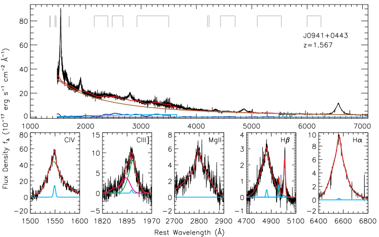
Fig. 1 shows an example of our global fits, and we tabulate the measured quantities in Table 2. Although with different fitting recipes, the continuum and emission line measurements are consistent with the measurements with SDSS spectra alone (Shen et al., 2011), and the largest discrepancy occurs for and : is systematically smaller by dex, and is systematically larger by dex, than the measurements in Shen et al. (2011). This is largely caused by the additional Balmer continuum model in the spectral fits. For simplicity, from now on we will by default refer to the broad line component when we mention the FWHM or luminosity of a particular line unless stated otherwise.
4. Results
We now proceed to examine correlations between continuum (line) luminosities and between line widths for different lines, as well as their virial products.
4.1. Luminosity Correlations
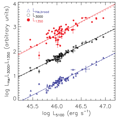
In Fig. 2 we compare different luminosities with the continuum luminosity at 5100 Å, and we list the slopes from the bisector linear regression fits using the BCES estimator (Akritas & Bershady, 1996) in Table 3. Our objects all have luminosity , and therefore contamination from host starlight is mostly negligible (e.g., Shen et al., 2011). For UV estimators, and (or ) are often used in replacement of . In addition, the luminosity of the broad H line is also used in pair with H line width (e.g., Greene & Ho, 2005). Since the original relation is calibrated against , a good correlation with is required to produce a reasonable estimate of the BLR size with alternative luminosity indicators. As shown in the top panel of Fig. 2, all three luminosity indicators are correlated with , where and are better correlated with than 333The measured with the Balmer continuum component in the fit is on average smaller by dex than that without fitting the Balmer continuum. However, both measurements of are tightly correlated with .. The slopes of these correlations are very close to unity, which means the ratios of these luminosities to almost do not depends on luminosity over this luminosity range.
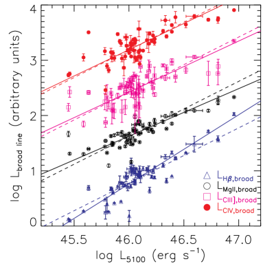
In cases where the continuum is too faint to detect or contaminated by host starlight or emission from a relativistic jet, an alternative route is to use the luminosity of the broad lines (e.g., Wu et al., 2004; Greene & Ho, 2005; Shen et al., 2011). The bottom panel of Fig. 2 shows correlations of different line luminosities with . Again, the H and Mg ii line luminosities seem to correlate with with lower scatter than CIII] and CIV. Interestingly, the scatter in the relation is comparable to that in the relation, suggesting that using the CIV line luminosity will not degrade the mass estimates much than using . The best-fit slopes of these correlations are slightly different from unity, indicating a possible mild luminosity dependence of the ratios of these luminosities to over this luminosity range.
We note that these luminosity correlations are not predominately caused by the common distance of each object. In fact, the dynamical range resulting from luminosity distances is only 0.4 dex given the limited redshift range of our objects, while the entire luminosity span is 1.5 dex. These luminosity correlations justify the usage of alternative luminosity indicators in various virial mass estimators. The scatter in the correlation between alternative luminosity indicator and will be one source of the scatter in virial mass estimates when compared with those based on H width and .
| Format | Units | Description | |
|---|---|---|---|
| objname | A10 | – | Object Name |
| F6.3 | continuum luminosity at restframe 1350 Å | ||
| Err | F6.3 | measurement error in | |
| F6.3 | continuum luminosity at restframe 3000 Å | ||
| Err | F6.3 | measurement error in | |
| F6.3 | continuum luminosity at restframe 5100 Å | ||
| Err | F6.3 | measurement error in | |
| F6.3 | luminosity of the broad CIV line | ||
| Err | F6.3 | measurement error in | |
| F6.3 | luminosity of the broad CIII] line | ||
| Err | F6.3 | measurement error in | |
| F6.3 | luminosity of the broad Mg ii line | ||
| Err | F6.3 | measurement error in | |
| F6.3 | luminosity of the broad H line | ||
| Err | F6.3 | measurement error in | |
| F6.3 | luminosity of the broad H line | ||
| Err | F6.3 | measurement error in | |
| I5 | FWHM of the broad CIV line | ||
| Err | I5 | measurement error in | |
| I5 | FWHM of the broad CIII] line | ||
| Err | I5 | measurement error in | |
| I5 | FWHM of the broad Mg ii line | ||
| Err | I5 | measurement error in | |
| I5 | FWHM of the broad H line | ||
| Err | I5 | measurement error in | |
| I5 | FWHM of the broad H line | ||
| Err | I5 | measurement error in | |
| I5 | blueshift of the broad CIV centroid w.r.t. the broad H centroid | ||
| Err | I5 | measurement error in | |
| I5 | blueshift of the broad CIV centroid w.r.t. the broad AlIII centroid | ||
| Err | I5 | measurement error in | |
| I5 | blueshift of the broad CIII] centroid w.r.t. the broad H centroid | ||
| Err | I5 | measurement error in | |
| I5 | blueshift of the broad Mg ii centroid w.r.t. the narrow [O iii] centroid | ||
| Err | I5 | measurement error in | |
| I5 | blueshift of the broad H centroid w.r.t. the narrow [O iii] centroid | ||
| Err | I5 | measurement error in | |
| I5 | blueshift of the broad H centroid w.r.t. the narrow [O iii] centroid | ||
| Err | I5 | measurement error in | |
| CIV AS | F4.2 | – | Asymmetry parameter of the broad CIV line |
Note. — Format of the tabulated spectral measurements. The full table is available in the online version.
| vs | Scatter | ||
|---|---|---|---|
| 1.044 | 0.099 | 0.13 | |
| 0.979 | 0.036 | 0.05 | |
| 1.010 | 0.042 | 0.07 | |
| 1.251 | 0.067 | 0.11 | |
| 0.861 | 0.070 | 0.11 | |
| 0.924 | 0.099 | 0.16 | |
| 0.950 | 0.085 | 0.14 |
Note. — and are the slope and uncertainty (1) in slope from the bisector linear regression fit of each luminosity against . The last column lists the scatter perpendicular to the best-fit linear relation (dominated by intrinsic scatter rather than measurement errors).
| with FWHMHβ | ||
| FWHMCIV | 0.11 | 0.39 |
| FWHMCIII] | 0.14 | 0.29 |
| FWHMMgII | 0.64 | |
| FWHMHα | 0.78 | |
| FWHMCIV,corr | 0.49 | |
| FWHMCIII],corr | 0.36 | |
| with | ||
| 0.02 | 0.89 | |
| -0.03 | 0.83 | |
| 0.21 | 0.11 | |
| EW CIV | -0.07 | 0.59 |
| 0.59 | ||
| 0.36 | ||
| CIV AS | -0.28 | 0.028 |
Note. — is the Spearman rank-order coefficient and is the probability of being drawn from random distributions. FWHMCIV,corr and FWHMCIII],corr are the corrected FWHMs using the linear regression fits shown in Fig. 6.
4.2. Line Width Correlations


While it is still debated whether or not a narrow line component for CIV needs to be subtracted for high-redshift broad-line quasars (see discussions in, e.g., Bachev et al., 2004; Sulentic et al., 2007), it is clear that narrow CIV emission does exist, as seen in some type 2 quasars (e.g., Stern et al., 2002). The [O iii] coverage in our near-IR spectra makes it possible to constrain the strength of the narrow CIV emission by fixing its line width and velocity offset to those of the narrow [O iii] lines. We have measured the width of CIV with and without the subtraction of a possible narrow line component. In Fig. 3 we compare the resulting CIV FWHM with the two methods. The two objects with large error bars (J10090230 and J15421112) have associated absorption, which causes some ambiguities in decomposing the CIV line in our Monte Carlo mock spectra and therefore leads to large uncertainties (see §3). We found that the narrow line contribution to CIV is generally weak for objects in our sample, and only in 2 objects (J11192332 and J17106023) the narrow CIV component is strong enough to make a large difference in the line width measurement. From now on we use the CIV line width with narrow line subtraction. We note, however, that our quasars are luminous, and the relative strength of the narrow CIV emission may be larger for lower luminosity objects (see, e.g., Bachev et al., 2004; Sulentic et al., 2007).
In the bottom panel of Fig. 3 we compare the CIV FWHM and CIII] FWHM. The measurement errors are typically larger for CIII] due to the ambiguity of decomposing the CIII] complex, but a correlation is still seen between the FWHMs of CIV and CIII]. This is intriguing because CIII] does not show as large a blueshift relative to the low-ionization lines as does CIV (e.g., Richards et al., 2011, Shen et al., in preparation) when the contributions from SiIII] and AlIII are removed. In Fig. 4 we plot the FWHM against the velocity offset relative to the broad H line, for CIV and CIII] respectively. In both cases a significant positive correlation is detected, i.e., FWHM increases with blueshift. Such a trend is already known when comparing CIV and Mg ii (e.g., Shen et al., 2008, 2011), and now it is confirmed when comparing CIV directly with H. However, similar trends were not found for the FWHM of H, H or Mg ii against their velocity shift relative to [O iii]. We also tested if there is any correlation between FWHM and other properties (continuum luminosity, color, line asymmetry) for all five lines and found none of them is significant.

In Fig. 5 we plot different line widths against the broad H FWHM. We have suppressed measurement errors in these plots for clarity. In addition to the traditional FWHM, we also measure the full-width-at-third-maximum (FWTM) and full-width-at-quarter-maximum (FWQM) as alternative line width indicators. Consistent with earlier studies, we see strong correlations among the widths of H, H and Mg ii (e.g., Greene & Ho, 2005; Salviander et al., 2007; Shen et al., 2008; Wang et al., 2009). On the other hand, both CIII] and CIV line widths show poor correlations with H line width. Table 4 lists the Spearman rank-order coefficients of these correlations. Since we found using FWTM and FWQM does not improve the correlations, we will focus on FWHM from now on.
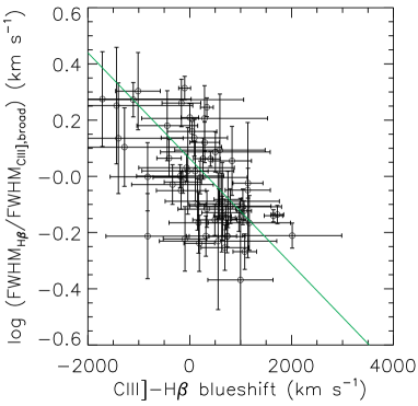


These results suggest that CIV and CIII] have different kinematics from Mg ii and the Balmer lines, and possibly originate from a different region than the low-ionization lines. However, since some dispersion in the CIV and CIII] FWHM is driven by the blueshift (e.g., Fig. 4), accounting for this dependence may reduce the difference in FWHM between CIV/CIII] and the low-ionization lines. To test this, we plot the difference in FWHM , as a function of the blueshift with respect to Hfor CIII] and CIV, in Fig. 6 (top panels). The green lines are the linear regression results using the Bayesian method of Kelly (2007). We then use these best-fit linear relations to correct for the observed CIII] and CIV FWHMs:
| (2) |
where is the blueshift relative to H, and and are the best-fit coefficients of the linear regression shown in green lines in the top panels of Fig. 6; for CIII], and for CIV. The “corrected” CIII] and CIV FWHMs are plotted against the broad H FWHMs in the bottom panels of Fig. 6. This time significant correlations are detected for both CIII] and CIV, and CIV has the most significant improvement (see Table 4 for Spearman rank-order coefficients). Nevertheless, there is still substantial scatter ( dex for CIII] and dex for CIV) among these correlations. This “irreducible” scatter probably again reflects the different origins of CIII] and CIV from the low-ionization lines, which makes it difficult to bring their line widths into good agreement. We will return to this point in §5.1.
Although the blueshift relative to H seems a viable proxy to correct the CIII] and CIV FWHM to better agree with the H FWHM, it is of little practical value. One would like a proxy that can be determined from regions around the CIII] or CIV line alone. We have tried to correlate with , , asymmetry parameters of CIV (defined as , where is the peak flux wavelength, and and are the wavelengths at half peak flux from the model fits), and blueshift relative to AlIII. We found that is best correlated with asymmetry parameters of CIV and the blueshift relative to AlIII at the level, although still worse than the ones against the blueshift relative to H (where ). Using these weak correlations to correct for CIV FWHM does not seem to reduce the scatter between the CIV and H FWHM much.
| Type | offset | Ref | ||||
|---|---|---|---|---|---|---|
| (dex) | (dex) | |||||
| Fiducial mass | ||||||
| 0.91 | 0.5 | 2 | – | – | VP06 | |
| Previous calibrations | ||||||
| 0.774 | 0.520 | 2.06 | 0.01 | 0.14 | A11 | |
| 1.239 | 0.430 | 2.10 | 0.15 | S11 | ||
| 0.895 | 0.520 | 2.00 | 0.03 | 0.003 | A11 | |
| 1.676 | 0.560 | 2.00 | 0.07 | GH05 | ||
| 0.860 | 0.500 | 2.00 | 0.02 | 0.16 | VO09∗ | |
| 0.740 | 0.620 | 2.00 | 0.17 | 0.17 | S11∗ | |
| 1.933 | 0.630 | 2.00 | 0.22 | 0.16 | S11∗ | |
| 0.660 | 0.530 | 2.00 | 0.10 | 0.40 | VP06 | |
| 1.525 | 0.457 | 2.00 | 0.09 | 0.38 | S11 | |
| This work | ||||||
| () | ||||||
| 1.390 | 0.555 | 1.873 | 0.01 | 0.12 | – | |
| 2.216 | 0.564 | 1.821 | 0.008 | 0.15 | – | |
| 1.963 | 0.401 | 1.959 | 0.02 | 0.04 | – | |
| 1.816 | 0.584 | 1.712 | 0.02 | 0.16 | – | |
| 3.979 | 0.698 | 1.382 | 0.03 | 0.15 | – | |
| 7.295 | 0.471 | 0.242 | 0.03 | 0.28 | – | |
| 7.535 | 0.639 | 0.319 | 0.002 | 0.26 | – | |
| SDSS quasars | ||||||
| () | ||||||
| 0.963 | 0.468 | 2.010 | 0.02 | 0.16 | – |
Note. — Virial BH mass calibrations of Eq. (3) based on different line width and luminosity combinations for the 60 objects in our sample, calibrated against the VP06 FWHM-based H virial masses. References of previous calibrations: GH05 (Greene & Ho, 2005), VP06 (Vestergaard & Peterson, 2006), VO09 (Vestergaard & Osmer, 2009), S11 (Shen et al., 2011), A11 (Assef et al., 2011). For each calibration we measure the average offset and scatter relative to the fiducial mass by fitting a Gaussian to the mass residual . The scatter in the mass residual is dominated by intrinsic scatter than by measurement errors. ∗In using the Mg ii calibrations in Shen et al. (2011) and Vestergaard & Osmer (2009) we have added dex to the measured and subtracted dex from the measured to account for the different fitting recipe used in this work. Note that the absolute uncertainties of these calibrations are on the level of dex (e.g., Peterson, 2011).
4.3. Comparing Single-Epoch Virial Mass Estimators

The investigations so far in the previous two sections treated luminosity and line width independently. In principle, if there is covariance between line width and luminosity when comparing the virial products based on different lines, the resulting scatter in the residual virial products may be increased or reduced. Since we did not observe any strong dependence of line width on luminosity for any particular line, we expect such effects to be modest at most.
As reasoned in the introduction, we adopt the H virial masses as the “truth” values, and minimize the differences using alternative line estimator with respect to H. There is more than one calibration based on and (e.g., McLure & Dunlop, 2004; Vestergaard & Peterson, 2006; Assef et al., 2011), and we use the Vestergaard & Peterson (2006, VP06) calibration as our standard, which is compatible with our measurements of the H FWHM, and provides similar estimates to those using the calibration in Assef et al. (2011, see below). The virial mass estimator based on a particular pair of line width and luminosity is:
| (3) |
where and FWHM are the continuum (or line) luminosity and width for the specific line, and coefficients , and are to be determined by linear regression analysis.
In order to minimize the difference in virial masses compared to our fiducial masses, we allow the slopes on both luminosity and FWHM to vary. We use the multi-dimensional Bayesian linear regression method in Kelly (2007) to perform regression, treating our standard masses as the dependent variable , and as the 2-dimensional independent variable . This approach takes into account measurement errors, and possible covariance between luminosity and FWHM, thus is arguably better than regressions on versus and versus separately. The regression results are listed in Table 5.
In Fig. 7 we show the comparisons between different virial mass estimators and the VP06 H estimator. We show in the first two columns the comparisons for several calibrations in earlier work, and in the last two columns the comparisons for our new calibrations as summarized in Table 5.
These earlier calibrations were calibrated using fainter samples than probed here, but in general they provide mass estimates that agree with the fiducial H-based virial masses (mean offset dex). The exceptions are the Mg ii-based calibrations in Shen et al. (2011), where the steeper slope of the relation for Mg ii than for H has led to increasingly larger discrepancies towards high luminosities444We note that the Mg ii calibrations in Shen et al. (2011) were not based on linear regression fits against H masses, and had a slope in the relation fixed to be the one in McLure & Dunlop (2004). Using a steeper slope 0.62 in relation, the Mg ii virial masses in Shen et al. (2011) have negligible systematic offset relative to both H-based masses at and CIV-based masses at . . For our new calibrations, the slope on FWHM is close to (albeit slightly smaller than) 2 for H, H and Mg ii, indicating that using FWHM in these calibrations improves the agreement with our standard mass estimator (VP06-H). However, for CIV, our linear regression result has a slope on FWHM that is much shallower. This is because CIV FWHM is poorly correlated with H FWHM for our sample, and the scatter between the two FWHMs rather than between the two continuum luminosities is the dominant source of the difference in their virial masses (in contrast to Assef et al., 2011, see discussions in §5.1); therefore the regression prefers a smaller dependence on CIV FWHM to minimize the difference in the two mass estimates. In other words, the individual CIV FWHM adds little to improve the agreement with our standard mass estimates, but instead degrades the agreement. We found similar trends for CIII] (not shown) as for CIV.
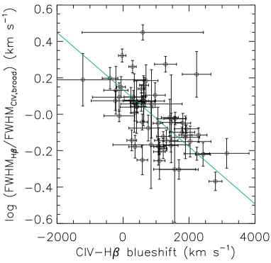
We test the dependence of the CIV virial mass residual on continuum luminosity, color and line shifts. The mass residual is correlated with , but this is expected since both masses involve luminosity. Correcting for this color dependence only marginally improves the agreement between the two masses. On the other hand, the dependence on CIV-H blueshift is strong enough such that incorporating this dependence can improve the agreement between CIV masses and the standard masses. These results again reflect the fact that the difference in FWHM is the dominant source in the virial mass difference. But this correction based on the CIV-H blueshift is of little practical use since there is no need to correct CIV-based virial masses if we have H coverage. Using the CIV-AlIII blueshift or CIV asymmetry as a surrogate for the CIV-H blueshift only leads to marginal improvement of the CIV-based masses, and thus is not of much practical value either.
Our new calibrations for Mg ii yield consistent mass estimates as those estimated from H for luminous () quasars. However, it would be useful to derive a Mg ii calibration that is also applicable to lower luminosities. For this purpose we select quasars from the compilation in Shen et al. (2011) with good H and Mg ii measurements ( dex) and (to reduce host contamination). We combine these quasars with the high-luminosity quasars in our sample and perform the two-dimensional linear regression on against the fiducial H-based masses. The best-fit coefficients are listed in Table 5. This Mg ii calibration is close to the one presented in Vestergaard & Osmer (2009), and works reasonably well for the entire luminosity regime .
5. Discussion
5.1. Comparison with Earlier Studies
There have been many studies comparing different virial mass estimators (e.g., Vestergaard & Peterson, 2006; McGill et al., 2008; Dietrich & Hamann, 2004; Dietrich et al., 2009; Netzer et al., 2007; Shen et al., 2008, 2011; Wang et al., 2009). These comparison studies used samples that have different sizes, spectral quality, luminosity and redshift ranges, and focused on different lines. The current work is among the few studies that simultaneously investigate CIV through H in the same objects, and our sample is substantially larger and more homogeneous than used in similar studies (e.g., Dietrich & Hamann, 2004; Dietrich et al., 2009).
Our results agree with earlier work that the line width of Mg ii is well correlated with that of H (e.g., Salviander et al., 2007; McGill et al., 2008; Shen et al., 2008), but now we have extended this conclusion to higher luminosity than can be probed with earlier samples at lower redshift. On the other hand, we confirm the poor correlation between CIV FWHM and H FWHM reported earlier (e.g., Baskin & Laor, 2005; Netzer et al., 2007), which was also inferred from the comparison between CIV and Mg ii using SDSS quasars (e.g., Shen et al., 2008).
Assef et al. (2011) used a sample of high-redshift quasars with optical (covering CIV) and near-IR (covering the Balmer lines) spectroscopy to show that there is a correlation between the widths of CIV and the Balmer lines. They further concluded that the correlation persists, although it becomes weaker, when other objects compiled from Vestergaard & Peterson (2006), Netzer et al. (2007) and Dietrich et al. (2009) are included.
The Assef et al. (2011) sample is small (only 9 objects with all the measurements available for Spearman tests), and they do not probe a large dynamic range in CIV blueshift (see their fig. 13). The lack of large CIV blueshift objects in their sample probably explains why they did not detect a significant correlation between the CIV virial mass residual and the CIV blueshift.
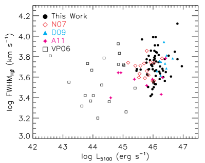
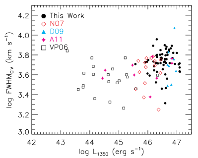
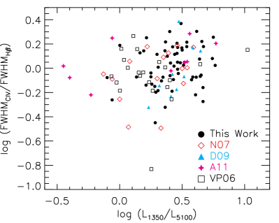
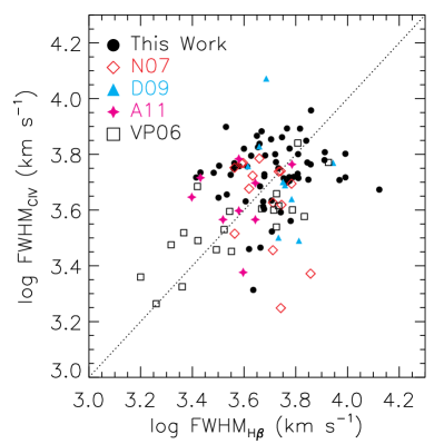
To further investigate the disagreement on the correlation between CIV and H FWHMs, we collected luminosity and FWHM measurements from Assef et al. (2011, 9 objects; A11), Vestergaard & Peterson (2006, 21 objects; VP06), Netzer et al. (2007, 15 objects; N07), and Dietrich et al. (2009, 9 objects; D09). We use the Prescription A measurements of CIV FWHM in Assef et al. (2011). Fig. 8 shows their distribution in the luminosity-FWHM space. The VP06 sample probes a much lower luminosity regime than the other high-redshift samples. In the bottom panel of Fig. 8 we also show the ratio of against the continuum luminosity ratio (optical-UV color). The A11 sample spreads over a larger range in continuum color than the other samples, including several objects that are much redder than typical quasars (e.g., Richards et al., 2003). Only the D09 and A11 samples show a mild correlation between FWHM ratio and optical-UV color, with Spearman rank-order coefficients of 0.65 () and 0.67 (), respectively. This correlation helps to reduce the virial mass differences between CIV and H once this color effect is taken out (Assef et al., 2011).
In Fig. 9 we show the comparison between CIV and H FWHMs for different samples. We run Spearman tests for the combined sample and for each subsample, and find that the correlation between the CIV and H FWHMs reported in Assef et al. (2011) is essentially driven by objects in the VP06 sample, which probes a much fainter luminosity than other samples as indicated in Fig. 8. None of the other samples show significant correlations between the two FWHMs, and this result does not change when we restrict ourselves to high-quality measurements. These high-redshift samples have a narrower dynamic range in line width than the VP06 sample, and thus the intrinsic scatter between the CIV and H FWHMs can easily wash out any weak correlation. We therefore reinforced our earlier conclusion in §4.2 that, at least for the high-luminosity objects, the CIV FWHM is poorly correlated with the H FWHM.
5.2. Implications for High-Redshift Quasars
The comparisons between different line estimators in previous sections suggest that in the absence of Balmer lines, the Mg ii estimator can be used as a substitute, which will yield consistent virial mass estimates to those based on the Balmer lines. On the other hand, CIV and CIII] can be used, although using the individually measured CIV/CIII] FWHM does not seem to offer much advantage over simply using a constant value; of course, this conclusion is valid for the high-luminosity regime probed by this study. CIV is a complicated line, and may be more affected by a non-virial component as luminosity increases (see discussions in Richards et al., 2011). These unusual properties of CIV suggest that it is likely the least reliable virial mass estimator at high-redshift, thus optical/near-IR coverage of Mg ii or the Balmer lines is desired for reliable virial mass estimates (e.g., Netzer et al., 2007; Trakhtenbrot et al., 2011; Marziani & Sulentic, 2011).
One should also be aware that even for the most reliable H-based virial mass estimates, there is still considerable scatter between virial masses and true masses (on the level of dex, e.g. Peterson, 2011). Rare objects with unusual continuum and/or emission line properties (for instance, dust reddened quasars, e.g., Richards et al., 2003) will lead to additional uncertainty in these virial mass estimates, along with measurement errors from poor spectral quality. Recognizing and accounting for the uncertainties in these virial mass estimates is crucial in essentially all BH mass related studies (e.g., Shen et al., 2008; Kelly et al., 2009, 2010; Shen & Kelly, 2010, 2012).
6. Summary
In this paper we have empirically determined the relations between single-epoch virial mass estimators based on different lines for luminous () quasars, using a sample of 60 intermediate-redshift quasars with complete coverage from CIV through H with good optical and near-IR spectroscopy. Our sample consists of typical quasars with no peculiarities in their continuum and emission line properties, has negligible contamination from host starlight, and is large enough to draw statistically significant conclusions. The main conclusions of this paper are the following:
-
•
The Mg ii FWHM is well correlated with the FWHM of the Balmer lines up to high luminosities (), which justifies the usage of Mg ii (in combination with or ) to estimate virial BH masses for luminous quasars at high redshift.
-
•
The narrow-line contribution to the CIV line is generally negligible for high-luminosity quasars; and the FWHMs of CIV and CIII] are well correlated, suggesting that both lines originate from similar regions.
-
•
The FWHM of CIV is poorly correlated with that of the Balmer lines, suggesting different BLRs for the CIV line and for the Balmer lines. Part of the discrepancy between the CIV and H FWHMs is correlated with the blueshift of CIV relative to H.
-
•
Using the FWHM of CIV increases the scatter between CIV and H based virial masses, which is at least true for the high luminosity regime probed in this study. CIII] does not seem to be a superior substitute for CIV, both because of the non-correlation between CIII] and H FWHMs, and because CIII] is blended with SiIII] and AlIII.
While in this work we focused on empirical relations, the correlations (and lack thereof) among these broad lines and continuum luminosities are ultimately determined by the accretion disk and BLR physics. In future work, we will use the same sample to investigate in more detail the emission line and continuum properties of intermediate-redshift quasars, such as the Baldwin effect (Baldwin, 1977), line centroid shifts, as well as average properties and correlations therein, in order to understand the underlying physics. In the mean time, we will expand our sample to include less luminous objects and test these correlations over a larger dynamic range in quasar luminosity.
References
- Akritas & Bershady (1996) Akritas, M. G., & Bershady, M. A. 1996, ApJ, 470, 706
- Assef et al. (2011) Assef, R. J., et al. 2011, ApJ, 742, 93
- Bachev et al. (2004) Bachev, R., Marziani, P., Sulentic, J. W., Zamanov, R., Calvani, M., & Dultzin-Hacyan, D. 2004, ApJ, 617, 171
- Bahcall et al. (1972) Bahcall, J. N., Kozlovsky, B.-Z., & Salpeter, E. E. 1972, ApJ, 171, 467
- Baldwin (1977) Baldwin, J. A. 1977, ApJ, 214, 679
- Baskin & Laor (2005) Baskin, A., & Laor, A. 2005, MNRAS, 356, 1029
- Bentz et al. (2006) Bentz, M. C., Peterson, B. M., Pogge, R. W., Vestergaard, M., & Onken, C. A. 2006, ApJ, 644, 133
- Blandford & McKee (1982) Blandford, R. D., & McKee, C. F. 1982, ApJ, 255, 419
- Boroson & Green (1992) Boroson, T. A., & Green, R. F. 1992, ApJS, 80, 109
- Cardelli et al. (1989) Cardelli, J. A., Clayton, G. C., & Mathis, J. S. 1989, ApJ, 345, 245
- Cohen et al. (2003) Cohen, M., Wheaton, W. A., & Megeath, S. T. 2003, AJ, 126, 1090
- Collin et al. (2006) Collin, S., Kawaguchi, T., Peterson, B. M., & Vestergaard, M. 2006, A&A, 456, 75
- Cushing et al. (2004) Cushing, M. C., Vacca, W. D., & Rayner, J. T. 2004, PASP, 116, 362
- Denney et al. (2009) Denney, K. D., Peterson, B. M., Dietrich, M., Vestergaard, M., & Bentz, M. C. 2009, ApJ, 692, 246
- Dibai (1980) Dibai, E. A. 1980, Soviet Ast., 24, 389
- Dietrich et al. (2002) Dietrich, M., Appenzeller, I., Vestergaard, M., & Wagner, S. J. 2002, ApJ, 564, 581
- Dietrich & Hamann (2004) Dietrich, M., & Hamann, F. 2004, ApJ, 611, 761
- Dietrich et al. (2009) Dietrich, M., Mathur, S., Grupe, D., & Komossa, S. 2009, ApJ, 696, 1998
- Fine et al. (2010) Fine, S., Croom, S. M., Bland-Hawthorn, J., Pimbblet, K. A., Ross, N. P., Schneider, D. P., & Shanks, T. 2010, MNRAS, 409, 591
- Gaskell (1982) Gaskell, C. M. 1982, ApJ, 263, 79
- Graham et al. (2011) Graham, A. W., Onken, C. A., Athanassoula, E., & Combes, F. 2011, MNRAS, 412, 2211
- Grandi (1982) Grandi, S. A. 1982, ApJ, 255, 25
- Greene & Ho (2005) Greene, J. E., & Ho, L. C. 2005, ApJ, 630, 122
- Greene & Ho (2007) —. 2007, ApJ, 667, 131
- Greene et al. (2010) Greene, J. E., Peng, C. Y., & Ludwig, R. R. 2010, ApJ, 709, 937
- Hewett & Wild (2010) Hewett, P. C., & Wild, V. 2010, MNRAS, 405, 2302
- Horne (1986) Horne, K. 1986, PASP, 98, 609
- Kaspi et al. (2007) Kaspi, S., Brandt, W. N., Maoz, D., Netzer, H., Schneider, D. P., & Shemmer, O. 2007, ApJ, 659, 997
- Kaspi et al. (2000) Kaspi, S., Smith, P. S., Netzer, H., Maoz, D., Jannuzi, B. T., & Giveon, U. 2000, ApJ, 533, 631
- Kelly (2007) Kelly, B. C. 2007, ApJ, 665, 1489
- Kelly et al. (2009) Kelly, B. C., Vestergaard, M., & Fan, X. 2009, ApJ, 692, 1388
- Kelly et al. (2010) Kelly, B. C., Vestergaard, M., Fan, X., Hopkins, P., Hernquist, L., & Siemiginowska, A. 2010, ApJ, 719, 1315
- Kelson (2003) Kelson, D. D. 2003, PASP, 115, 688
- Kollmeier et al. (2006) Kollmeier, J. A., et al. 2006, ApJ, 648, 128
- MacLeod et al. (2011) MacLeod, C. L., et al. 2011, arXiv:1112.0679
- Marziani & Sulentic (2011) Marziani, P., & Sulentic, J. W. 2011, arXiv:1108.5102
- McGill et al. (2008) McGill, K. L., Woo, J., Treu, T., & Malkan, M. A. 2008, ApJ, 673, 703
- McLure & Dunlop (2004) McLure, R. J., & Dunlop, J. S. 2004, MNRAS, 352, 1390
- McLure & Jarvis (2002) McLure, R. J., & Jarvis, M. J. 2002, MNRAS, 337, 109
- Metzroth et al. (2006) Metzroth, K. G., Onken, C. A., & Peterson, B. M. 2006, ApJ, 647, 901
- Murray et al. (1995) Murray, N., Chiang, J., Grossman, S. A., & Voit, G. M. 1995, ApJ, 451, 498
- Netzer et al. (2007) Netzer, H., Lira, P., Trakhtenbrot, B., Shemmer, O., & Cury, I. 2007, ApJ, 671, 1256
- Onken et al. (2004) Onken, C. A., Ferrarese, L., Merritt, D., Peterson, B. M., Pogge, R. W., Vestergaard, M., & Wandel, A. 2004, ApJ, 615, 645
- Park et al. (2012) Park, D., et al. 2012, ApJ, 747, 30
- Peterson (1993) Peterson, B. M. 1993, PASP, 105, 247
- Peterson (2011) Peterson, B. M. 2011, arXiv:1109.4181
- Peterson et al. (2004) Peterson, B. M., et al. 2004, ApJ, 613, 682
- Proga et al. (2000) Proga, D., Stone, J. M., & Kallman, T. R. 2000, ApJ, 543, 686
- Rafiee & Hall (2011a) Rafiee, A., & Hall, P. B. 2011a, MNRAS, 825
- Rafiee & Hall (2011b) —. 2011b, ApJS, 194, 42
- Reichert et al. (1994) Reichert, G. A., et al. 1994, ApJ, 425, 582
- Richards et al. (2003) Richards, G. T., et al. 2003, AJ, 126, 1131
- Richards et al. (2011) Richards, G. T., et al. 2011, AJ, 141, 167
- Salviander et al. (2007) Salviander, S., Shields, G. A., Gebhardt, K., & Bonning, E. W. 2007, ApJ, 662, 131
- Schlegel et al. (1998) Schlegel, D. J., Finkbeiner, D. P., & Davis, M. 1998, ApJ, 500, 525
- Schneider et al. (2010) Schneider, D. P., et al. 2010, AJ, 139, 2360
- Sesar et al. (2007) Sesar, B., et al. 2007, AJ, 134, 2236
- Shen et al. (2008) Shen, Y., Greene, J. E., Strauss, M. A., Richards, G. T., & Schneider, D. P. 2008, ApJ, 680, 169
- Shen et al. (2011) Shen, Y., et al. 2011, ApJS, 194, 45
- Shen & Kelly (2010) Shen, Y., & Kelly, B. C. 2010, ApJ, 713, 41
- Shen & Kelly (2012) —. 2012, ApJ, 746, 169
- Simcoe et al. (2010) Simcoe, R. A., et al. 2010, SPIE Conf., 7735, 38
- Skrutskie et al. (2006) Skrutskie, M. F., et al. 2006, AJ, 131, 1163
- Stern et al. (2002) Stern, D., et al. 2002, ApJ, 568, 71
- Sulentic et al. (2007) Sulentic, J. W., Bachev, R., Marziani, P., Negrete, C. A., & Dultzin, D. 2007, ApJ, 666, 757
- Sulentic et al. (2000) Sulentic, J. W., Marziani, P., & Dultzin-Hacyan, D. 2000, ARA&A, 38, 521
- Trakhtenbrot et al. (2011) Trakhtenbrot, B., Netzer, H., Lira, P., Shemmer, O. 2011, ApJ, 730, 7
- Tsuzuki et al. (2006) Tsuzuki, Y., Kawara, K., Yoshii, Y., Oyabu, S., Tanabé, T., & Matsuoka, Y. 2006, ApJ, 650, 57
- Vacca et al. (2003) Vacca, W. D., Cushing, M. C., & Rayner, J. T. 2003, PASP, 115, 389
- Vestergaard (2002) Vestergaard, M. 2002, ApJ, 571, 733
- Vestergaard et al. (2008) Vestergaard, M., Fan, X., Tremonti, C. A., Osmer, P. S., & Richards, G. T. 2008, ApJ, 674, L1
- Vestergaard & Osmer (2009) Vestergaard, M., & Osmer, P. S. 2009, ApJ, 699, 800
- Vestergaard & Peterson (2006) Vestergaard, M., & Peterson, B. M. 2006, ApJ, 641, 689
- Vestergaard & Wilkes (2001) Vestergaard, M., & Wilkes, B. J. 2001, ApJS, 134, 1
- Wandel et al. (1999) Wandel, A., Peterson, B. M., & Malkan, M. A. 1999, ApJ, 526, 579
- Wang et al. (2009) Wang, J., et al. 2009, ApJ, 707, 1334
- White et al. (1997) White, R. L., Becker, R. H., Helfand, D. J., & Gregg, M. D. 1997, ApJ, 475, 479
- Wilson et al. (2004) Wilson, J. C., et al. 2004, SPIE Conf., 5492, 1295
- Wilhite et al. (2007) Wilhite, B. C., Brunner, R. J., Schneider, D. P., & Vanden Berk, D. E. 2007, ApJ, 669, 791
- Woo (2008) Woo, J.-H. 2008, AJ, 135, 1849
- Woo & Urry (2002) Woo, J.-H., & Urry, C. M. 2002, ApJ, 579, 530
- Woo et al. (2010) Woo, J.-H., et al. 2010, ApJ, 716, 269
- Wu et al. (2004) Wu, X.-B., Wang, R., Kong, M. Z., Liu, F. K., & Han, J. L. 2004, A&A, 424, 793