CERN-PH-TH/2012-054
Tuning supersymmetric models at the LHC:
A comparative analysis at two-loop level.
D. M. Ghilencea, H. M. Lee, M. Park111E-mail: dumitru.ghilencea@cern.ch, hyun.min.lee@cern.ch, myeonghun.park@cern.ch
a Theory Division, CERN, 1211 Geneva 23, Switzerland.
b Theoretical Physics Department, National Institute of Physics
and Nuclear Engineering Bucharest (IFIN-HH), MG-6 077125 Romania.
Abstract
We provide a comparative study of the fine tuning amount () at the two-loop leading log level in supersymmetric models commonly used in SUSY searches at the LHC. These are the constrained MSSM (CMSSM), non-universal Higgs masses models (NUHM1, NUHM2), non-universal gaugino masses model (NUGM) and GUT related gaugino masses models (NUGMd). Two definitions of the fine tuning are used, the first () measures maximal fine-tuning wrt individual parameters while the second () adds their contribution in “quadrature”. As a direct consequence of two theoretical constraints (the EW minimum conditions), fine tuning () emerges at the mathematical level as a suppressing factor (effective prior) of the averaged likelihood () under the priors, under the integral of the global probability of measuring the data (Bayesian evidence ). For each model, there is little difference between , in the region allowed by the data, with similar behaviour as functions of the Higgs, gluino, stop mass or SUSY scale () or dark matter and constraints. The analysis has the advantage that by replacing any of these mass scales or constraints by their latest bounds one easily infers for each model the value of , or vice versa. For all models, minimal fine tuning is achieved for near GeV with a to depending on the model, and in the CMSSM this is actually a global minimum. Due to a strong ( exponential) dependence of on , for a Higgs mass near GeV, the above values of increase to between and . Possible corrections to these values are briefly discussed.
1 Introduction
Low energy (TeV-scale) supersymmetry (SUSY) can provide a solution to the hierarchy problem. This is done without undue amount of electroweak scale fine tuning () that is present in the non-supersymmetric theories like the Standard Model (SM). A large value of this is just another face of the hierarchy problem (for a review see [1] and references therein). However, negative searches for superpartners increase the SUSY scale () which in turn can increase . In the extreme case when is very high ( TeV) one recovers the scenario of non-supersymmetric theories (SM, etc) with a large . In the light of current negative SUSY searches at the LHC it is useful to examine in detail the amount of fine tuning that supersymmetric models need, as a test of SUSY as a solution to the hierarchy problem. The alternative is to ignore this problem and adopt an effective theory approach, with a low effective cutoff (few TeV) that, unlike SUSY, does not detail the “new physics” at/beyond this scale. Such models usually have a relative to the TeV scale comparable to that of SUSY models relative to the Planck scale.
While a small value of (say less than ) is desirable, the exact value still accepted for a solution to the hierarchy problem is rather subjective. Even worse, there are also different definitions of in the literature. Two common definitions are
| (1) |
are new parameters (of mass dimension 1), that SUSY introduces in the model (shown above for the CMSSM). was the first measure used [2], but is also common. Two definitions for can lead to different predictions and the absence of a widely accepted upper value for it is another problem. To avoid these issues, we compute both and and compare their implications in generic SUSY models, without an upper bound on them (to be fixed by the reader). This is one of the main purposes of this work.
These measures of fine tuning were introduced more on physical intuition than rigorous mathematical grounds so another important purpose is to clarify their link with other approaches and find technical support. Both provide a local measure (in the space ) of the quantum cancellations and help to decide which phase space points of a model are less fine tuned (more probable). When actually comparing models, a more global measure would be desirable. Our scan over the whole parameter space when evaluating ’s will alleviate this issue. But one question remains: what is the relation of to other (global) measures of the success of SUSY in solving the hierarchy problem? To answer this, consider the Bayesian probability density of a point in parameter space given the data :
| (2) |
Here is the likelihood the parameters fit the data and is a global normalization factor called Bayesian “evidence”. For two models with the same data and priors , the ratio of their gives their relative overall probability. So a large is needed to decide that a model is more probable than another. Then what is the relation between and fine-tuning? As it was observed in [3] (see also [4]), when integrating over one parameter of the theory (in this case ), following an experimental constraint (on ), there is an emergent effective prior which brings in a fine tuning penalty for points with large222Note however that fine tuning wrt is not dominant in CMSSM for higgs mass above GeV [5]. [3]. These points then have little contribution to because . A larger can then indicate a preference for points of lower , and the link of with fine tuning wrt individual parameters is apparent.
We explore this idea further and evaluate by investigating the effect of the theoretical constraints that received less attention: we refer to the two minimum conditions of the potential. Further, the above observation and the need to evaluate clearly suggests to integrate over all parameters (and we shall do so), and also over nuisance variables, which are parameters already present in the SM (like Yukawa couplings [3, 6]). The result is that so is actually preferred by the Bayesian evidence calculation. Then receives contributions mostly from points of small , but this also depends on the priors and . To conclude, the inverse of acts as an extra, effective prior in (2) and is indeed a physical quantity with impact on global . This clarifies the exact, mathematical link of overall fine tuning wrt all parameters , to and the Bayesian evidence .
With this technical motivation, we then evaluate the fine tuning for generic models, using both definitions and ; this is done in a two-loop leading log numerical analysis that provides the state-of-the-art analysis of the fine tuning in the models considered, consistent with current data. Interestingly, the results we find are little dependent on the definition used for , with and showing similar behaviour and values. This is important since it is usually thought that different fine tuning measures should give different results. Our results correspond to a scan over the entire parameter space of the models (including ). This is an extremely CPU-intensive task, made possible by the CERN batch computing service. The analysis of , is done for the following models:
a) - CMSSM: the constrained minimal supersymmetric standard model. For a recent
b) - NUHM1: a CMSSM-like model but with equal Higgs soft masses, different from .
c) - NUHM2: as for CMSSM but with different Higgs soft masses and different from .
d) - NUGM: a CMSSM-like model but with non-universal gaugino masses.
e) - NUGMd: a benchmark NUGM model [8] with a GUT relation among gaugino masses.
For these models our results are presented in a comparative way with , as functions of the lightest higgs, gluino, stop mass or the SUSY scale. Any experimental constraints on these can easily be used to identify , for that model. On top of these plots various contour lines corresponding to the remaining masses, dark matter or the constraints are shown. Such comparative analysis for different models and definitions of was not done in the past and has the advantage that it can be updated by the latest data, without re-doing the whole analysis. In particular, for each model we identify the corresponding ’s for a Higgs mass of GeV that seems favoured by Atlas and CMS [9, 10]. We shall see such value requires to depending on the model, and uncertainties in are also discussed. In all cases is minimal near GeV. For ways to have GeV with smaller fine-tuning in SUSY models see [1, 11].
2 Fine tuning, and the role of theoretical constraints.
Before our numerical analysis, we re-examine the relation between the Bayesian probability of a point in parameter space or the evidence and the EW scale fine tuning, in models with theoretical constraints. Without loss of generality, we do this for the constrained MSSM (CMSSM). This analysis extends a previous similar study of this problem of [3] (Section 2 in both papers), see also [4]. To place this discussion on quantitative grounds consider the CMSSM scalar potential
| (3) | |||||
The couplings and the soft masses receive one- and two-loop corrections that for the MSSM can be found in [12, 13]. Let us introduce the notation
| (4) |
where .
When testing a model such as the CMSSM, one imposes two classes of constraints: theoretical and experimental. Let us discuss them. Minimizing this scalar potential leads to two theoretical constraints given below and their solutions for are the same as those of the eqs where and are introduced for later convenience:
| (5) |
Here is a combination of vev’s of , . The order of the arguments of is relevant later, while the dots denote other parameters (other Yukawa or gauge couplings,…) present at one-loop and beyond, that we ignore in this section only, without loss of generality.
As a result of these two constraints, the EW minimum solutions for and become functions of the (mass dimension 1) parameters of the model which for CMSSM are shown above, in a standard notation. When discussing fine tuning, usually only the first constraint in (5) is considered, although the second is equally important, as our result for will show. These constraints fixing , are assumed to be factorized out from the likelihood function and can be imposed by Dirac delta functions of arguments:
| (6) |
There is also a second class of constraints, that comes from the experiment, such as the accurate measurement of the masses of the top (), bottom () and boson (). Given the high accuracy of these measurements, one can assume some Gaussian distributions for the associated priors when evaluating the probability density or the evidence . However, for a more qualitative analysis and to good approximation one can again implement these constraints (likelihood) by Dirac delta functions of suitable arguments
| (7) |
where are experimental values. One can consider similar constraints for and gauge couplings but for simplicity we do not do that (their implementation is similar).
When testing the SUSY models with a given set of parameters (such as for CMSSM), one should in principle marginalize (i.e. integrate) the density over the “nuisance” parameters. Examples of these nuisance parameters are those already present in the Standard Model. These are the Yukawa couplings [3, 6] which were restricted (in the analysis of this section only) to the simpler case of top and bottom Yukawa couplings. Other parameters to integrate over are the dependent parameters: the vev and which can (in principle) take any value, until fixed by minimization constraints (5), (6), also (7) for .
To compare two SUSY models, one should compare their evidence for similar priors and data . To compute , one integrates over all parameters (of the SM and those mentioned above) and over as well, with chosen priors . For the CMSSM case, after imposing the above constraints with the corresponding priors, one finds
| (8) | |||||
where is the likelihood of fitting the given data (D) with a particular set of values ; i=1,…5, etc; the priors and are not known, but logarithmic or flat priors are common choices for individual parameters. Regarding the priors and , these are already included and given by the corresponding Dirac delta’s shown in (6), (7). We integrated over rather than over the corresponding masses . This is a possible choice, preferable because the masses are derived quantities, see discussion in [3]. Finally, leaving aside the integral over and , the above equation simply gives the probability density .
The important point about eq.(8) is that now all parameters that we integrated over can be regarded as arbitrary, since the constraints that render them dependent variables are implemented by the Dirac delta functions associated to the theoretical and experimental constraints. is a function of the CMSSM parameters, but also of the nuisance parameters () and . Finally is a normalization constant not important below.
To evaluate , one uses , , and after performing the integrals over and one finds
| (9) | |||||
with where () is the gauge couplings of U(1) (SU(2)) and
| (10) |
Integrating over333We use with the derivative wrt evaluated in ; is the unique root of ; we apply this to a function for with the root . :
| (11) | |||||
Above denotes the partial derivative wrt the variable of the function of arguments: , where (10) is used. The curly bracket is evaluated at the unique root of the second minimum condition in (5) of the scalar potential: . Through this condition, becomes a function of the independent parameters , as usual (one can eventually trade for , as often done, but we do not do this here). In the last step we converted the integral into a surface integral444One uses with where is defined by and is in basis . Another form of (11) is found by replacing , by their values in space (instead of ) and removing the product in integral (11). where is the surface defined by the equation while is the surface element in the parameter space . Recall that is one minimum condition which together with the second one (or ) control the value of . A notation was used where has the arguments shown and is the gradient in coordinate space .
The important result is that contains a suppression factor where we denoted
| (12) |
with
| (13) |
Note that contains a derivative of evaluated at , so it encodes the effects of variations about the ground state of both minimum conditions (5), see the two Dirac ’s in (9). A good stability of these conditions under such (quantum) variations requires small . Interestingly we also notice that so is preferred by the calculation of the Bayesian evidence . The points of smaller , give larger contribution to , but this also depends on or priors. We can say that is an extra effective prior, emerging when marginalizing over parameters, subject to the theoretical constraints. With , points of large pay the fine-tuning cost and so have a small impact on . The latter is then used to decide which of two models is more probable.
For further illustration, assume log priors for Yukawa couplings and for SUSY parameters , using and with . Then
| (14) |
To conclude, is an extra effective prior of the model and emerges as a measure of fine tuning. In the general case can be read from (11), (2) and the link between and the Bayesian evidence is clear. Numerical studies of or should then include such effect due to the two theoretical constraints. To our knowledge this effect was so far overlooked in such studies.
Note that that emerges in eqs.(2), (14), does not contain partial derivatives wrt Yukawa couplings. This is because these are nuisance (SM-like) parameters that were integrated out, so are included as a global effect. Also, such parameters are not part of the new ones () that SUSY introduces, so it is no surprise that they are not explicitly manifest in or in the denominator under integrals (2), (14).
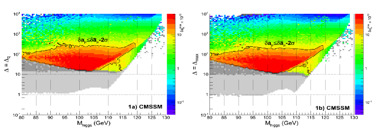
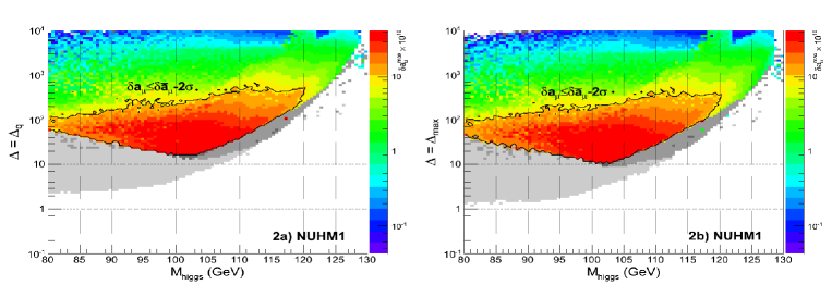
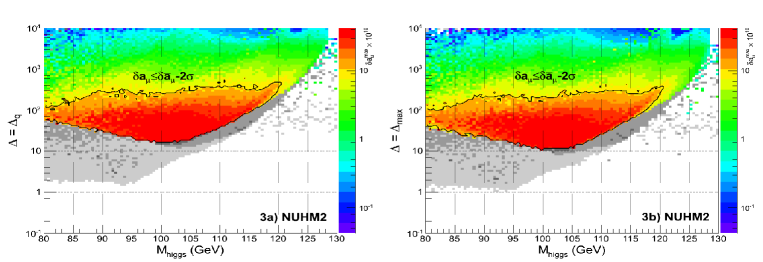
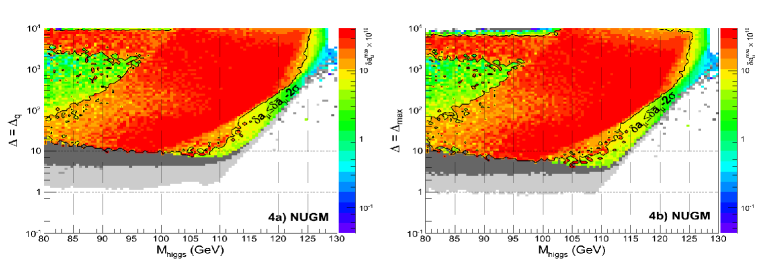
Figures 1 to 4: , versus ; lightest grey (0) area: excluded by SUSY mass bounds; darker grey (1): excluded by , , ; dark grey (2): excluded by condition . Coloured area: allowed by data and ; is shown colour encoded. Area outside contour: (). Red area (inside): largest is within of .
These above results bring technical support to a physical meaning of the fine tuning. They show that it is desirable to have a smaller , as also expected from physical considerations. Again, one should remember that this may not always be the region from where receives the largest contributions, as this depends also on the priors, the integral(s) or their measure. Note also that changing the priors of the nuisance parameters or the measure can give different values for Bayesian although with enough data one expects this dependence to become weaker. With this technical motivation for the fine tuning measures and their relation to , below we study the values of , for many SUSY models.
3 Numerical results for in generic supersymmetric models.
We present our numerical results for and in a comparative analysis for generic models used for SUSY searches at the LHC. We scan the entire parameter space of the models, consistent with the theoretical constraints, using a two-loop leading-log analysis. and are presented as functions of physical scales (mass of higgs, stop, gluino, SUSY scale ) with constraints (muon magnetic momentum , dark matter abundance ). The models considered are:
the CMSSM model, of parameters . Then is that shown in (1) and (13), evaluated at the two-loop leading log level. See [5] for a recent study, whose results were recovered by this work.
the NUHM1 model: this is a CMSSM-like model but with Higgs masses in the ultraviolet (uv) different from , , with parameters . Then is as in (13) with summation over this set.
the NUHM2 model: this is a CMSSM-like model with non-universal Higgs mass, , with independent parameters . Then is that of (13) with summation over this set.
the NUGM model: this is a CMSSM-like model with non-universal gaugino masses , , with , . Then is given by (13) with the sum over this set.
the NUGMd model: this is a special case of NUGM-like model with a relation among the gaugino masses , , of the type , where take only discrete, fixed values. Such relations can exist due to some GUT symmetries, like SU(5), SO(10), etc. The particular relation we consider is a benchmark point of [8] with , , , corresponding to a particular GUT (SU(5)) model, see Table 2 in [8]. As a result, is that of (13) with .
In all models we also evaluate the alternative definition of given by
| (15) |
and where the set is listed above for each model.
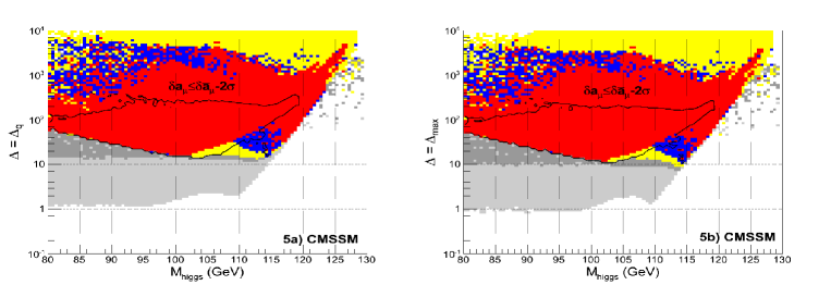
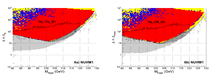
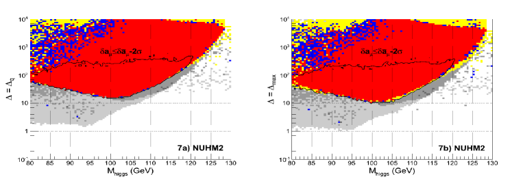
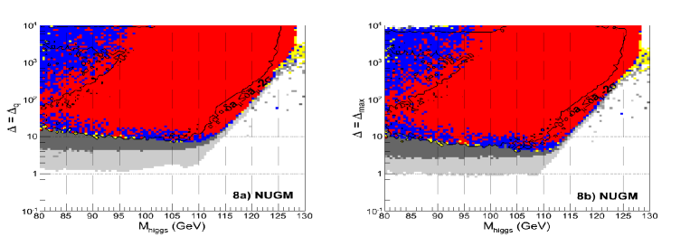
Figures 5 to 8: , versus : Various grey areas and values: as for Figures 1 to 4. Colored ares: allowed by data other than . Blue area: . Red area ( saturation). Yellow: .
Before presenting our results let us describe the method used. The scan over the full phase space of each model was done using Pythia 8 [14] random number generator. The public code micrOMEGAs 2.4.5 [15] and SoftSusy 3.2.4 code [16] were then used, with the latter adapted to compute for all models the fine tuning of the electroweak scale at the two-loop leading log level (instead of its default, one-loop calculation). This includes two-loop tadpoles to the two electroweak minimum conditions. The data output was then filtered by the experimental constraints. The run time to generate the phase space points of the five models was about 15000 one-day jobs on the CERN computing service, and each plot was generated from points in a random scan of the parameter space (for alternative and recent data analysis see [17]).
| Experimental constraints | Values used |
|---|---|
| SUSY particle masses | Routine in micrOmegas 2.4.5,“MSSM/masslim.c” |
| Muon magnetic moment | at [18]. |
| process | at [19]. |
| process | at [20]. |
| -parameter | at [21]. |
| Dark matter relic density | at [22]. |
Our results555 After this work was completed, an updated bound on was published [23]. We checked that our fine tuning estimates are unchanged, for a higgs mass in the now preferred region of 122 GeV to 128 GeV. shown in the plots allow the reader to set his own constraints on physical scales such as the higgs mass, gluino, stop mass or SUSY scale , or dark matter abundance and infer from that the amount of fine tuning. Note also that the LEP2 bound on is never imposed on our figures, and we let the reader to do this, in the light of future LHC results666 Note that a flat bound like LEP2 bound on should be used with care since it applies only to SM.. This has the great advantage that the impact of future bounds from LHC on these physical scales can very easily be seen on the plots, without the need to re-do the whole analysis. Space constraints do not allow us to also present a description of the allowed parameter space used in these plots, due to complicated correlations among these, that can only be presented as more additional figures, that we postpone to a future work. Finally, the parameter space () that we scanned over was: TeV, TeV, TeV and also . All plots are marginalized over and .
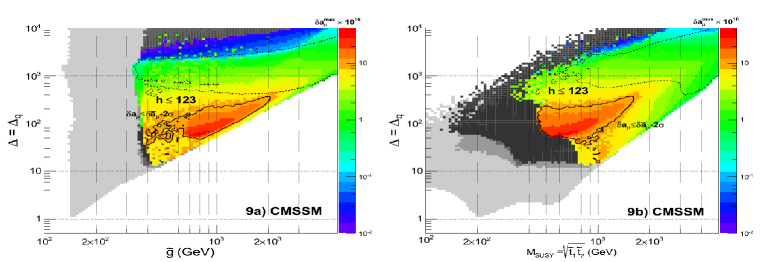
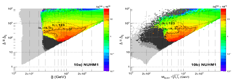
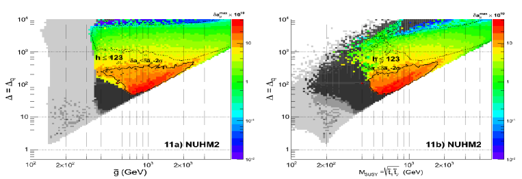
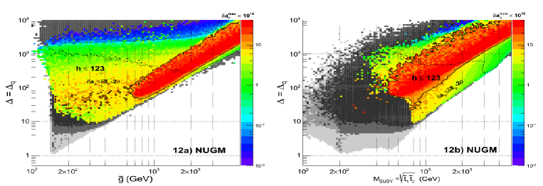
Figures 9 to 12: versus gluino (left) and SUSY scale (right) for various models; GeV in area below the dotted line; similar plots exist for ; various grey areas as in Figures 1 to 4, forbidden by data. Black area: or GeV. Outside the red area: ; inside this area is within of . See also caption of Figs 1-4.
3.1 versus and the values of .
In figs. 1 to 4 a), b) and 17 a), b), we show the plots for and as functions of the mass of the lightest Higgs boson , for all models: CMSSM, NUHM1, NUHM2, NUGM, NUGMd. The impact of constraint is also shown with a contour line displaying an island of its largest values, within of . For other values ( deviations, etc), the largest is also shown colour encoded, see the scale on the right side of the plots. The lightest grey (level 0) areas in these plots are excluded by the lower bounds on the spartners masses obtained from negative SUSY searches. The darker grey (level 1) areas are excluded by , and constraints. The dark grey area (level 2) that we also show, visible only for NUGM model corresponds to and has and is present at GeV. This region is excluded by demanding , (), preferred by data.
As it is shown in these figures, the LEP2 bound (114.4 GeV) [24] on the higgs mass was not imposed. Note however that above this value both ’s are largely independent of the experimental data (ignoring ) for all models other than NUHM1, NUHM2; these still have some dependence on data (the small grey area). This is interesting and suggests that the range of values of , can be fixed mainly by theory and the higgs mass bound, with little or no impact from other data.
As it is seen from these results, the differences between and are practically negligible. For a given model and a fixed Higgs mass, there is a relative factor between 1 and 2 and which can be safely ignored777 In general no individual dominates clearly for all higgs masses, see fig.2 in [5] for the CMSSM.. There is also very similar behavior i.e. various contour lines such as that of maximal are nearly identical for both , . This is interesting and shows that one can use either definition for fine tuning to obtain a rather similar result.
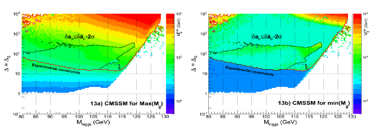
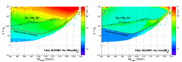
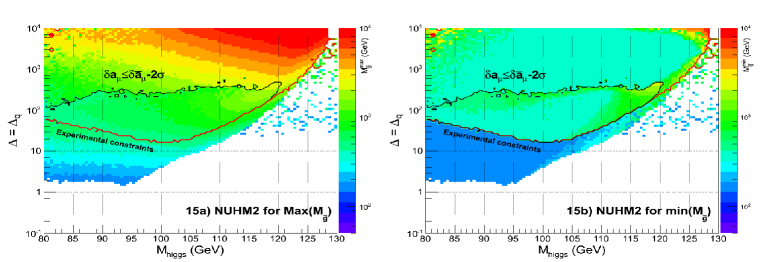
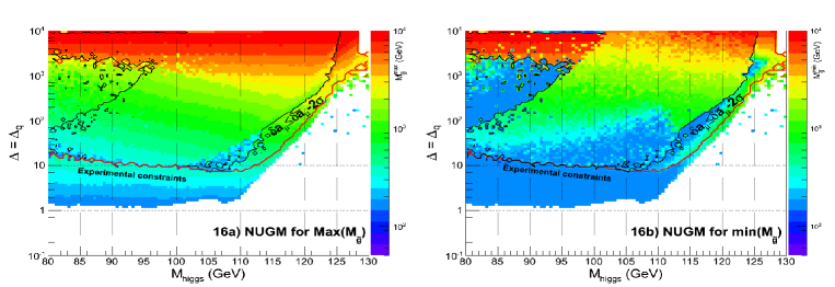
Figures 13 to 16: versus with largest (left plots) and lowest (right plots) gluino mass; For given one infers the gluino mass range. Area allowed by data (except ) as shown above the continuous line, see also Figures 1-4. Values as large as are outside the closed contour; inside the contour: largest is within of and the gluino mass satisfies it.
In the CMSSM the minimal value of and is situated for higgs mass near the LEP2 value as also discussed in [5]. This means that to respect the LEP2 bound on the Higgs mass there is no fine tuning cost due to quantum corrections. This corrects common but wrong opposite claims in the literature. Further, if one accepted the principle that of a model should actually be minimized, then one immediately has a CMSSM prediction for GeV without using experimental constraints (ignoring here ), for details see [5]888There is a GeV theoretical uncertainty from the various public codes [16, 25, 26].. In models other than CMSSM and after imposing the LEP2 bound, the fine tuning is again smallest near this scale. For near GeV, to , depending on the model. Above this mass value, both , grow very fast ( exponentially), due to the quantum corrections to the Higgs mass (which are logarithmic in ). As a result, for the currently interesting region discussed by CMS and Atlas experiments [9, 10], of GeV, there is significant amount of fine tuning required, to ; for GeV, to , depending on the model. From these results one could say that NUGM is preferable also because it could more easily comply with (). Finally, let us mention that a combined increase of and reduction of can reduce (best case scenario) the fine tuning for a fixed higgs mass by a factor near or so for the CMSSM [5], with similar effect expected for other models.
3.2 versus and dark matter relic density.
Let us now discuss the results of figures 5-8 a), b) and 18 a), b). These present the impact of the dark matter relic density constraint. Again, no significant difference between and is observed for the models considered. The meaning of light and dark grey areas is the same as in the previous figures. In blue we show points that are consistent with dark matter relic density within , i.e. these points have . The red points saturate the relic density within deviation from the central value. Finally, yellow points correspond to a relic density larger than that of the red points. Notice that with the exception of the CMSSM case at GeV region, for a higgs mass above this value one can easily saturate the relic density. This is true in particular for points near the 125 GeV region, although in CMSSM this may become more problematic (too large ).
The contour area of maximal values of already shown in previous figures 1-4, 17 is also presented. However, it should be stressed that points inside this contour area that have the dark matter abundance as shown (in blue, red or yellow) are not necessarily the same points that also have the largest within of ! (these are different projections on the 2D plane shown). However points that satisfy a relic density constraint and also have the largest within of experimental value do fall within a smaller area inside the contour shown. Of all models, NUGM could both saturate the relic density and fall within the contour line, for large range of higgs mass, although the fine tuning cost grows exponentially with . Figures 5a), b) and 8 a), b) show again that CMSSM and NUGM are the least sensitive models to any experimental constraints other than , for larger than GeV (negligible grey areas). Finally, since , are so similar, below we shall present only results for .
3.3 versus and versus .
So far we investigated the fine tuning as a function of the higgs mass. However, it is useful to present its dependence on other particles masses, and we do this for the gluino and the SUSY scale . This is useful since LHC searches for gluino or other SUSY partners can have a strong impact on fine tuning. This is seen in figures 9-12 a), b), and figures 19 a), b), where we show the dependence of on the gluino mass (figures a)) and on (figures b)) for all models. The light and dark grey areas have the same meaning as before, while the areas in black are ruled out by the higgs mass constraint GeV that we imposed (this allows 2-3 GeV uncertainty for at two-loop leading log level [16, 25, 26]). Contour (dotted) lines of a maximal value of 123 GeV of are displayed for all models: the points below this line respect this bound while those above can have larger values. The advantage of these plots is that if future data rules out GeV, the whole region below (outside) the dotted line (contour) will be removed from the plots, to leave a small, restrictive region.
is also shown in colour encoded areas, with a red island area showing the largest possible value with within of the experimental central value. Note again that the contour and the dotted line of upper bounds on higgs mass are different projections on the 2D plane of the figures. That means that points that have largest within of are not necessarily the same points that simultaneously have as large as 123 GeV. The impact of future gluino mass or bounds from the LHC can easily be seen on these plots, together with the associated fine tuning cost. The models NUGM and NUGMd relax the lowest bound on the gluino mass due to their non-universal gaugino masses.
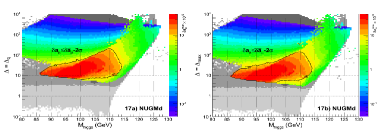
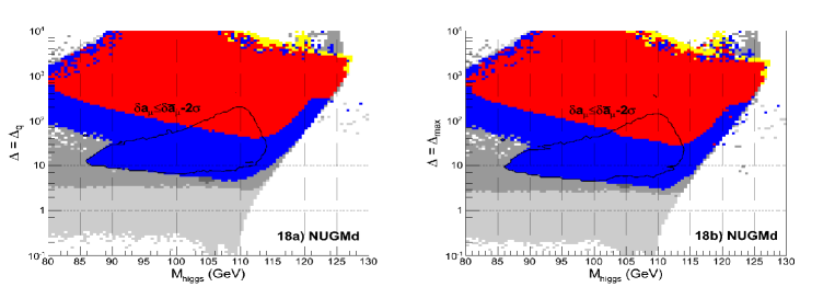
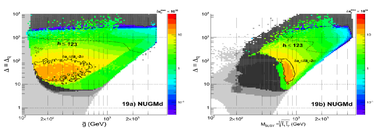
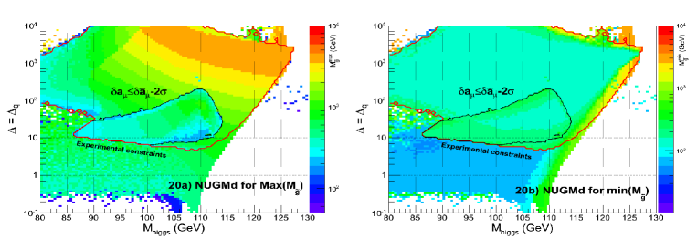
Figures 17-20: The benchmark NUGMd model: the description of the plots is identical to that in Figs. 1-17, but applied to NUGMd model, as follows: Figs 17 a), b) - as for figure 1 a), b). Figs 18 a), b) - as for figure 2 a), b). Figs 19 a), b) - as for figure 3 a), b). Figs 20 a), b) - as for figure 4 a), b).
3.4 versus and the gluino mass range.
A complementary presentation of the results of figures 1-4 a), 17 a) and figures 9-12 a), 19 a), b) is that of figures 13-16 a), b) and 20 a), b). In these is presented again as a function of the higgs mass, but with the gluino mass as a parameter, with its largest value in plots a) and lowest possible value in plots b), see the colour encoded scale. In this way one has a clear picture of the whole range of allowed values of gluino mass for a given and higgs mass. Intermediate values of gluino mass are colour encoded. For the large , above 125 GeV the gluino mass tends to be larger (above 1 TeV), and within a narrow range, with increasing fine tuning cost. The range of values of gluino is rather similar in CMSSM, NUGM or in NUHM1, NUHM2.
One important remark about the contour of largest shown: the gluino mass range shown inside this contour respects all experimental constraints, including the constraint of (within )! If this constraint is lifted, the range of gluino mass, for a fixed higgs mass and fine tuning, would be larger. This also explains the sudden change of colour/spectra of gluino masses around the contour line of as compared to region immediately outside the contour.
3.5 Stop versus gluino mass, with the largest and minimal .
For a future comparison with results from LHC searches for new physics, we also present in figures 21, the dependence stop versus gluino mass and with the largest value of Higgs mass that is possible with the former two fixed. The minimal fine tuning cost that comes with this is also shown in the corresponding areas (bordered by red contour lines), while the largest allowed is colour encoded, see the scale on the right side of the plots. The latest bounds on the gluino and stop masses can be translated into (upper) bounds for the higgs mass. Currently, stop-gluino exclusion plots from the LHC exist only for simple models that cannot be used for comparison [27], see the first plot in figure 21. Eventually, at very large gluino and stop masses the (minimal) fine tuning cost becomes too large and the models may be considered unrealistic. It can be seen from these plots how the lowest allowed fine tuning increases as the higgs mass goes towards its upper limit. If one rules out values of fine tuning of say one immediately removes the area outside the contour line that borders this region, to leave a significantly smaller area of correlation stop-gluino-higgs mass.
While the CMSSM, NUHM1, NUHM2 are more restricted by superpartners masses (excluded light grey areas), in the case of the NUGM and NUGMd, not surprisingly, the impact of the spartners mass bounds is small (since the universality condition was relaxed). Again, the NUGM model is less restricted, allowing a large higgs mass (125-128 GeV), with a stop as light as GeV and gluino mass between TeV.
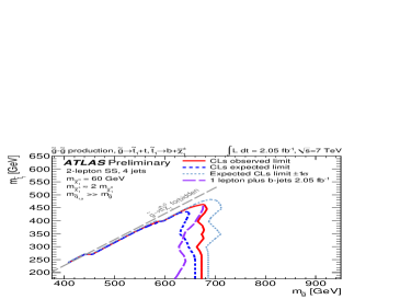
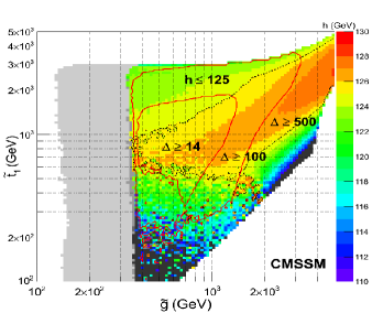
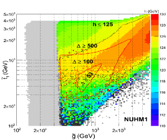
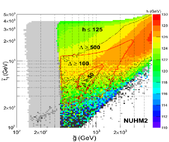
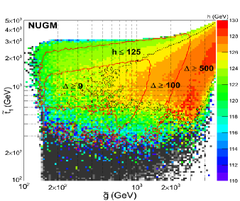
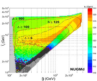
Figure 21:
Top left plot: Atlas stop-gluino exclusion limits in a simple
supersymmetric model [27].
Rest of the plots:
The dependence stop vs gluino mass in CMSSM, NUHM1, NUHM2, NUGM, NUGMd
models, in this order. We present the lowest value of in
the areas where it is shown, bounded by red contour lines and
with no upper bound.
Areas of largest Higgs mass are also shown, colour encoded,
see the scale on the right side (minimal value: 111.4 GeV).
One can easily see the largest higgs mass and the
minimal fine tuning cost, for given gluino and stop masses.
Grey area is excluded by SUSY mass bounds. Black area is excluded by
imposing the constraint GeV and GeV.
This dependence can eventually be compared
with similar future plots from CMS/ATLAS searches.
4 Final remarks and conclusions
Low energy (TeV scale) supersymmetry is thought to solve the hierarchy problem without undue amount of fine tuning (). However there are different opinions on what the best definition for is, or what upper value is allowed for it while still claiming a SUSY solution to this problem. To avoid a subjective choice on these two issues, we performed a study of using two common definitions and and made no assumption about their largest allowed values. We also discussed the relation of to global probabilities (in the parameter space) to fit the data. We analyzed generic models: CMSSM, NUHM1, NUHM2, NUGM and a benchmark model, NUGMd, at two-loop leading log level, and both and were presented as functions of the higgs, gluino, stop mass or the SUSY scale, with additional constraints like dark matter or . The advantage of this comparative analysis is that using the figures for , , future experimental constraints can immediately be converted into an updated estimate for the fine tuning level of these models, without the need to re-do the whole analysis. The reader will then decide whether the amount of tuning so obtained is still acceptable for a solution to the hierarchy problem.
The measures of fine tuning were originally introduced more on physical intuition than rigorous mathematical grounds. In this work we provided mathematical support for the fine tuning via a quantitative relation to Bayesian evidence . As direct result of two theoretical constraints (EW min conditions), we showed that a fine tuning measure emerges as an additional suppression factor (effective prior) of the averaged likelihood under the initial priors, under the integral of global probability of measuring the data (the evidence ). So the Bayesian evidence calculation prefers as a fine tuning measure. As a result, the evidence therefore points of large (strongly fine tuned) have little or no impact on the global probability of the model to fit the data. These results provide technical support to the idea that fine tuning has a physical meaning and that preferably it should have small values in realistic models for the corresponding point in the parameter space.
Our numerical results for and as functions of the higgs mass, showed that they have close values for the same higgs mass and also very similar behaviour for all models considered. There is a small discrepancy factor between them (between 1 and 2) which is most visible for regions of the higgs mass that are anyway excluded by the data. All these results show a good independence on the actual definition used for fine tuning. For GeV there is a relative independence of or on the experimental constraints (other than ) for CMSSM or NUGM, NUGMd, with a minor dependence for NUHM1, NUHM2. So in this case , are largely controlled by theoretical constraints. Also, the dark matter relic density can in all cases be saturated within of the current value.
The dependence of both on the gluino mass or on the SUSY scale shows a similar behaviour for all models. The CMSSM, NUGM and NUGMd models show a lower amount of fine tuning for the same experimental constraints, and NUGM can even accommodate () and GeV, however in this case there is always a fine tuning cost. As our plots showed, for the CMSSM no fine tuning amount can reconcile () values considered (i.e. contour at in the plots), with a GeV region which is situated outside this contour. For a Higgs mass near GeV, the fine tuning is of order in all models other than NUGM, NUGMd where it is of order . There is a strong (roughly exponential) variation of with . A reduction of 2 GeV of can bring down both ’s to to , depending on the model. For GeV, to and in the CMSSM this corresponds to a global minimum. Finally, let us mention that the combined effect of a increase of the top mass and a similar reduction of the measured strong coupling at EW scale can reduce the fine tuning for a given by a factor near 2 or so in the CMSSM case [5]. Although we did not studied it here (due to long CPU runs), we expect similar effect for the other models. This is because Yukawa corrections help radiative EW breaking (reducing ) while QCD corrections have the opposite effect in the loop diagrams.
Are the values of fine tuning that we found too large? Based on previously agreed but highly subjective “reasonable” values of , the answer is probably affirmative. However, a clear answer is difficult, largely because depends exponentially on the higgs mass, so any small correction to it has a strong impact on . But comparing all models, for the same experimental constraints, there seems to be a preference for NUGM case when also considering the constraint. We let the reader to make his own opinion, based on the above results and figures and also on future LHC data (on gluino, higgs, stop and ) whose updated impact on our can easily be obtained. Also it should be kept in mind that very simple new physics beyond these SUSY models (like CMSSM with a gauge singlet with a TeV-scale SUSY mass term or a massive ) can lead to a very acceptable for a higgs mass as large as 130 GeV [11]. Further, subjective criteria also exist in other approaches that compare the probability of various models, such as those based on the Bayesian approach. Indeed, the evidence also has some dependence on the priors choice (flat, log, etc), until eventually more data can improve our knowledge of the models. We hope that the clear link between fine tuning and that we established together with our plots for both ’s will provide the starting point of a more detailed study.
References
- [1] S. Cassel and D. M. Ghilencea, “A Review of naturalness and dark matter prediction for the Higgs mass in MSSM and beyond,” Mod. Phys. Lett. A 27 (2012) 1230003 [arXiv:1103.4793 [hep-ph]].
- [2] J. R. Ellis, K. Enqvist, D. V. Nanopoulos and F. Zwirner, “Observables in Low-Energy Superstring Models,” Mod. Phys. Lett. A 1 (1986) 57.
- [3] M. E. Cabrera, J. A. Casas and R. Ruiz de Austri, “Bayesian approach and Naturalness in MSSM analyses for the LHC,” JHEP 0903 (2009) 075 [arXiv:0812.0536 [hep-ph]]. M. E. Cabrera, J. A. Casas and R. Ruiz d Austri, “MSSM Forecast for the LHC,” JHEP 1005 (2010) 043 [arXiv:0911.4686 [hep-ph]].
- [4] S. S. AbdusSalam, B. C. Allanach, F. Quevedo, F. Feroz and M. Hobson, “Fitting the Phenomenological MSSM,” Phys. Rev. D 81 (2010) 095012 [arXiv:0904.2548 [hep-ph]]. B. C. Allanach, K. Cranmer, C. G. Lester and A. M. Weber, “Natural priors, CMSSM fits and LHC weather forecasts,” JHEP 0708 (2007) 023 [arXiv:0705.0487 [hep-ph]]. B. C. Allanach, “Naturalness priors and fits to the constrained minimal supersymmetric standard model,” Phys. Lett. B 635 (2006) 123 [hep-ph/0601089].
- [5] S. Cassel, D. Ghilencea, G. G. Ross, “Testing SUSY at the LHC: Electroweak and Dark matter fine tuning at two-loop order,” Nucl. Phys. B 835 (2010) 110 [arXiv:1001.3884 [hep-ph]]. “Testing SUSY,” Phys. Lett. B 687 (2010) 214 [arXiv:0911.1134 [hep-ph]].
- [6] J.O. Berger, B. Liseo, R.L. Wolpert, “Integrated likelihood methods for eliminating nuisance parameters”, Statistical Science 1999, vol.14, No.1, 1-28.
- [7] P. H. Chankowski, J. R. Ellis and S. Pokorski, “The fine-tuning price of LEP,” Phys. Lett. B 423 (1998) 327 [arXiv:hep-ph/9712234]. P. H. Chankowski, J. R. Ellis, M. Olechowski and S. Pokorski, “Haggling over the fine-tuning price of LEP,” Nucl. Phys. B 544 (1999) 39 [arXiv:hep-ph/9808275]. G. L. Kane and S. F. King, “Naturalness implications of LEP results,” Phys. Lett. B 451 (1999) 113 [arXiv:hep-ph/9810374]. R. Barbieri and A. Strumia, “What is the limit on the Higgs mass?,” Phys. Lett. B 462 (1999) 144 [hep-ph/9905281]. R. Barbieri and A. Strumia, “About the fine-tuning price of LEP,” Phys. Lett. B 433 (1998) 63 [arXiv:hep-ph/9801353]. R. Barbieri and G. F. Giudice, “Upper Bounds on Supersymmetric Particle Masses,” Nucl. Phys. B 306 (1988) 63.
- [8] D. Horton and G. G. Ross, “Naturalness and Focus Points with Non-Universal Gaugino Masses,” Nucl. Phys. B 830 (2010) 221 [arXiv:0908.0857 [hep-ph]].
- [9] ATLAS Collaboration, F. Giannoti, “Update on the Standard Model Higgs searches in ATLAS,”. CERN Public Seminar, December 13, 2011, G. Aad et al. [ATLAS Collaboration], “Combined search for the Standard Model Higgs boson using up to 4.9 fb-1 of pp collision data at sqrt(s) = 7 TeV with the ATLAS detector at the LHC,” arXiv:1202.1408 [hep-ex]. [ATLAS Collaboration], “Search for the Standard Model Higgs boson in the diphoton decay channel with 4.9 fb-1 of pp collisions at sqrt(s)=7 TeV with ATLAS,” arXiv:1202.1414 [hep-ex]. [ATLAS Collaboration], “Search for the Standard Model Higgs boson in the decay channel H ZZ(*) 4l with 4.8 fb-1 of pp collisions at sqrt(s)=7 TeV with ATLAS,” arXiv:1202.1415 [hep-ex].
- [10] CMS Collaboration, G. Tonelli, “Update on the Standard Model Higgs searches in CMS,”. CERN Public Seminar, December 13, 2011, S. Chatrchyan et al. [CMS Collaboration], “Search for the standard model Higgs boson decaying to bottom quarks in pp collisions at sqrt(s)=7 TeV,” arXiv:1202.4195 [hep-ex]. S. Chatrchyan et al. [CMS Collaboration], “Search for neutral Higgs bosons decaying to tau pairs in pp collisions at sqrt(s)=7 TeV,” arXiv:1202.4083 [hep-ex]. S. Chatrchyan et al. [CMS Collaboration], “Search for the standard model Higgs boson decaying into two photons in pp collisions at sqrt(s)=7 TeV,” arXiv:1202.1487 [hep-ex]. S. Chatrchyan et al. [CMS Collaboration], “Combined results of searches for the standard model Higgs boson in pp collisions at sqrt(s) = 7 TeV,” arXiv:1202.1488 [hep-ex].
- [11] S. Cassel, D. M. Ghilencea and G. G. Ross, “Fine tuning as an indication of physics beyond the MSSM,” Nucl. Phys. B 825 (2010) 203 [arXiv:0903.1115 [hep-ph]]. G. G. Ross, K. Schmidt-Hoberg and F. Staub, “The generalised NMSSM at one loop: fine tuning and phenomenology,” arXiv:1205.1509 [hep-ph]; G. G. Ross and K. Schmidt-Hoberg, “The fine-tuning of the generalised NMSSM,” Nucl. Phys. B 862 (2012) 710. M. Carena, K. Kong, E. Ponton and J. Zurita, “Supersymmetric Higgs Bosons and Beyond,” Phys. Rev. D 81 (2010) 015001 [arXiv:0909.5434 [hep-ph]]. I. Antoniadis, E. Dudas, D. M. Ghilencea and P. Tziveloglou, “MSSM Higgs with dimension-six operators,” Nucl. Phys. B 831 (2010) 133 [arXiv:0910.1100 [hep-ph]]. I. Antoniadis, E. Dudas, D. M. Ghilencea and P. Tziveloglou, “Beyond the MSSM Higgs with d=6 effective operators,” Nucl. Phys. B 848 (2011) 1 [arXiv:1012.5310 [hep-ph]]. I. Antoniadis, E. Dudas, D. M. Ghilencea and P. Tziveloglou, “Non-linear MSSM,” Nucl. Phys. B 841 (2010) 157 [arXiv:1006.1662 [hep-ph]]. M. Carena, E. Ponton and J. Zurita, “BMSSM Higgs Bosons at the Tevatron and the LHC,” Phys. Rev. D 82 (2010) 055025 [arXiv:1005.4887 [hep-ph]]. M. Carena, E. Ponton and J. Zurita, “BMSSM Higgs Bosons at the 7 TeV LHC,” Phys. Rev. D 85 (2012) 035007 [arXiv:1111.2049 [hep-ph]]. A. Brignole, J. A. Casas, J. R. Espinosa and I. Navarro, “Low scale supersymmetry breaking: Effective description, electroweak breaking and phenomenology,” Nucl. Phys. B 666 (2003) 105 [hep-ph/0301121].
- [12] S. P. Martin and M. T. Vaughn, “Two Loop Renormalization Group Equations For Soft Supersymmetry Breaking Couplings,” Phys. Rev. D 50, 2282 (1994) [Erratum-ibid. D 78, 039903 (2008)] [arXiv:hep-ph/9311340].
- [13] M. S. Carena, J. R. Espinosa, M. Quiros and C. E. M. Wagner, “Analytical expressions for radiatively corrected Higgs masses and couplings in the MSSM,” Phys. Lett. B 355 (1995) 209 [arXiv:hep-ph/9504316].
- [14] T. Sjostrand, S. Mrenna, P. Z. Skands, “A Brief Introduction to PYTHIA 8.1,” Comput. Phys. Commun. 178 (2008) 852 [arXiv:0710.3820 [hep-ph]]. http://home.thep.lu.se/ torbjorn/pythiaaux/present.html
- [15] G. Belanger, F. Boudjema, A. Pukhov and A. Semenov, “MicrOMEGAs: A Program for calculating the relic density in the MSSM,” Comput. Phys. Commun. 149 (2002) 103 [hep-ph/0112278]. “micrOMEGAs: Version 1.3,” Comput. Phys. Commun. 174 (2006) 577 [hep-ph/0405253]. “MicrOMEGAs 2.0: A Program to calculate the relic density of dark matter in a generic model,” Comput. Phys. Commun. 176 (2007) 367 [hep-ph/0607059].
- [16] B. C. Allanach, “SOFTSUSY: a program for calculating supersymmetric spectra,” Comput. Phys. Commun. 143 (2002) 305 [hep-ph/0104145].
- [17] O. Buchmueller, R. Cavanaugh, A. De Roeck, M. J. Dolan, J. R. Ellis, H. Flacher, S. Heinemeyer and G. Isidori et al., “Supersymmetry in Light of 1/fb of LHC Data,” arXiv:1110.3568 [hep-ph]. S. Sekmen, S. Kraml, J. Lykken, F. Moortgat, S. Padhi, L. Pape, M. Pierini and H. B. Prosper et al., “Interpreting LHC SUSY searches in the phenomenological MSSM,” arXiv:1109.5119 [hep-ph]. S. Cassel, D. M. Ghilencea, S. Kraml, A. Lessa, G. G. Ross, “Fine-tuning implications for complementary dark matter and LHC SUSY searches,” [arXiv:1101.4664 [hep-ph]]. S. Akula, N. Chen, D. Feldman, M. Liu, Z. Liu, P. Nath and G. Peim, “Interpreting the First CMS and ATLAS SUSY Results,” arXiv:1103.1197 [hep-ph]. D. Feldman, K. Freese, P. Nath, B. D. Nelson and G. Peim, “Predictive Signatures of Supersymmetry: Measuring the Dark Matter Mass and Gluino Mass with Early LHC data,” arXiv:1102.2548 [hep-ph]. P. Bechtle, K. Desch, H. K. Dreiner, M. Kramer, B. O’Leary, C. Robens, B. Sarrazin, P. Wienemann, “What if the LHC does not find supersymmetry in the sqrt(s)=7 TeV run?,” [arXiv:1102.4693 [hep-ph]]. S. Akula, D. Feldman, Z. Liu, P. Nath, G. Peim, “New Constraints on Dark Matter from CMS and ATLAS Data,” [arXiv:1103.5061 [hep-ph]]
- [18] M. Davier, A. Hoecker, B. Malaescu, C. Z. Yuan and Z. Zhang, “Reevaluation of the hadronic contribution to the muon magnetic anomaly using new e+ e- pi+ pi- cross section data from BABAR,” Eur. Phys. J. C 66 (2010) 1 [arXiv:0908.4300 [hep-ph]].
- [19] D. Asner et al. [Heavy Flavor Averaging Group Collaboration], “Averages of b-hadron, c-hadron, and -lepton Properties,” arXiv:1010.1589 [hep-ex].
- [20] The CMS and LHCb Collaborations, CMS-PAS-BPH-11-019, LHCb-CONF-2011-047, CERN-LHCb-CONF-2011-047.
- [21] The Particle Data Group, http://pdg.lbl.gov/
- [22] G. Hinshaw et al. [WMAP Collaboration], “Five-Year Wilkinson Microwave Anisotropy Probe (WMAP) Observations: Data Processing, Sky Maps, and Basic Results,” Astrophys. J. Suppl. 180 (2009) 225 [arXiv:0803.0732 [astro-ph]].
- [23] R. Aaij et al. [LHCb Collaboration], “Strong constraints on the rare decays and ,” arXiv:1203.4493 [hep-ex].
- [24] S. Schael et al. [ALEPH and DELPHI and L3 and OPAL and LEP Working Group for Higgs Boson Searches Collaborations], “Search for neutral MSSM Higgs bosons at LEP,” Eur. Phys. J. C 47 (2006) 547 [hep-ex/0602042]. R. Barate et al., “Search for the standard model Higgs boson at LEP,” Phys. Lett. B 565 (2003) 61 [hep-ex/0306033].
- [25] G. Degrassi, S. Heinemeyer, W. Hollik, P. Slavich, and G. Weiglein, “Towards high precision predictions for the MSSM Higgs sector,” Eur.Phys.J. C28 (2003) 133, arXiv:hep-ph/0212020 [hep-ph].
- [26] S. Heinemeyer, “MSSM Higgs physics at higher orders,” Int.J.Mod.Phys. A21 (2006) 2659, arXiv:hep-ph/0407244 [hep-ph].
- [27] The ATLAS collaboration, ATLAS-CONF-2012-004 “Search for gluinos in events with two same-sign leptons, jets and missing transverse momentum with the ATLAS detector in collisions at 7 TeV”