Updated templates for the interpretation of LHC results on supersymmetry in the context of mSUGRA
Abstract
In this short note, we describe the preparation of updated templates for the interpretation of SUSY results from the LHC in the context of mSUGRA. The standard plane is shown for fixed and = 173.2 GeV. Two scenarios are considered: (1) GeV and and (2) GeV and . In each case, the universal scalar mass parameter varies in the range GeV, while the universal gaugino mass parameter varies in the range GeV. We delineate notable regions in parameter space, including the region with a charged LSP (stau), the LEP2 reach, and the cosmologically preferred region with 100% neutralino dark matter. The templates also show mass contours for a few key particles (gluino, squark and Higgs boson). The mass spectrum is calculated with the SoftSusy-3.2.4 package, while the neutralino relic density is obtained with MicrOMEGAs version 2.4.
I Introduction
Low energy supersymmetry (SUSY) Golfand:1971iw ; Ramond:1971gb ; Neveu:1971rx ; Neveu:1971iv ; Volkov:1973ix ; Wess:1973kz ; Wess:1974tw ; Fayet:1977yc is a primary target of the LHC collaborations in their quest for new physics at the TeV scale. Unfortunately, even the most minimal supersymmetric extension of the Standard Model comes with a large number of a priori unknown parameters (superpartner masses, mixing angles and CP violating phases). The experimental exploration of such a large parameter space is impractical. Therefore, it has become customary to present experimental limits from searches for supersymmetry in terms of simple benchmark models with very few input parameters, see e.g. Battaglia:2001zp ; Allanach:2002nj ; Battaglia:2003ab ; Allanach:2006st ; AbdusSalam:2011fc . The most popular SUSY benchmark model is the minimal supergravity (mSUGRA) model Chamseddine:1982jx ; Barbieri:1982eh ; Hall:1983iz , a.k.a. the “constrained MSSM” (cMSSM). In this model the SUSY mass parameters are input at the grand unification (GUT) scale, conventionally defined as the scale where the two gauge couplings and meet. At the GUT scale, all scalars in the model have a common mass , while all gaugino fermion superpartners have a common mass . The model has two additional continuous parameters: , a common trilinear scalar coupling at the GUT scale, and , the ratio of the two Higgs vacuum expectation values, plus a discrete parameter, the sign of the higgsino mass parameter . In order to obtain the physical SUSY mass spectrum, the parameters , and are evolved via the renormalization group equations (RGEs) from the GUT scale down to the electroweak scale, where the radiatively corrected mass spectrum is computed. Since the gauge and Yukawa couplings of the Standard Model are input at the electroweak scale, the procedure must be iterated until it converges on a stable solution. There are several state of the art, publicly available codes on the market which can do these calculations, and they generally give similar results in the bulk of the parameter space Allanach:2003jw . Here we use the SoftSusy-3.2.4 software package softsusy .
| Parameter | Value | |
|---|---|---|
| 0.1184 | ||
| 127.934 | ||
| 173.2 GeV | ||
| 4.2 GeV | ||
| sign() | + | |
| 0 GeV | -500 GeV | |
| 10 | 40 | |
In this note we provide details of the design of mSUGRA templates which can be used for interpretation of supersymmetry searches at the LHC. Given the ubiquitousness of the mSUGRA model, it has become customary to present exclusion limits from SUSY searches in the parameter plane Baer:1994nc , for fixed values of the remaining mSUGRA (and Standard Model) parameters (shown in Table 1). In anticipation of the improved reach with 2011 and 2012 data, we extend the previously considered ranges of and , allowing them to vary in GeV and GeV, correspondingly. Two different slices are considered. The first has a moderate value of , while is taken to be . The second slice has a higher value of and a different GeV. In each case, the sign of the parameter is positive, and the top mass is taken to be GeV. In what follows, we refer to these two scans by their respective parameters.
II mSUGRA templates
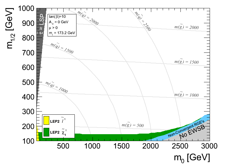
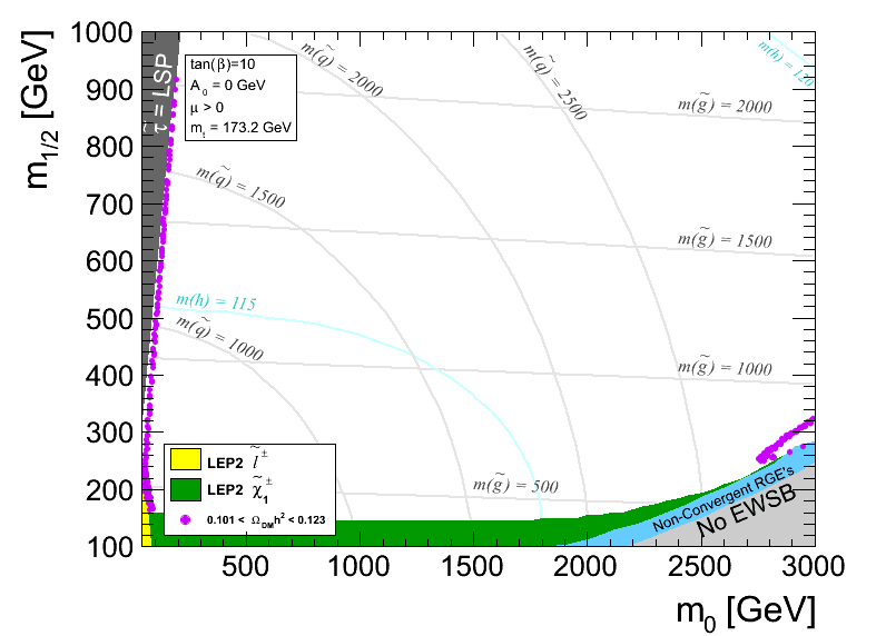
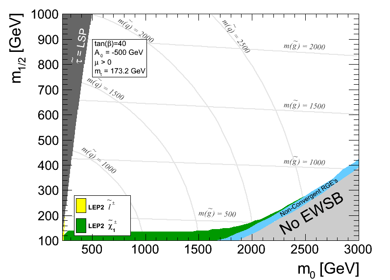
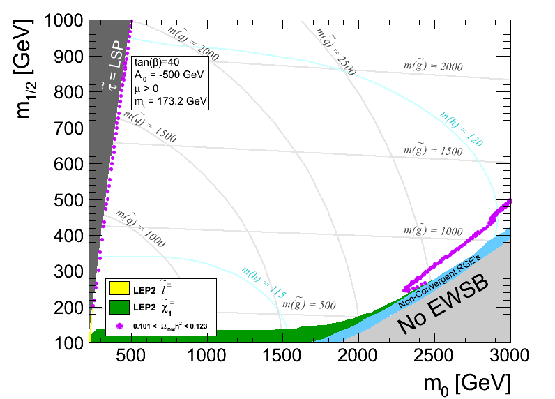
We begin by presenting the templates in their final form before discussing the details of their respective features. The templates are displayed in Figs. 1 and 2 for and , respectively. The calculations are performed across an grid. The LHC mSUGRA scans CMSscan sample this grid in 20 GeV intervals for both and with about 10k events for each point. A finer granularity is of course desirable but is computationally prohibitive, as each grid point has to be propagated through the generation, simulation, and reconstruction chain. The storage space required for hosting these datasets would also grow quadratically with finer granularity. Since our goal is to simply provide a canvas which delineates theoretical and experimental regions of interest in the plane, we only need to make use of the mass spectrum calculations, and these come in concise SLHA files from the SoftSusy output. This allows us to pursue a much finer granularity of 5 GeV intervals. In the high scan, grid points with GeV do not yield a suitable neutral dark matter candidate, thus the scan effectively begins at GeV.
III Constraints on the mSUGRA parameter space
Within the mSUGRA parameter space considered here, there are regions which are not considered to be viable for hypothesis testing, since they are subject to constraints imposed by theory or experiment.
III.1 Theoretical constraints
III.1.1 Charged LSP
One nice feature of the mSUGRA model is that throughout most of the parameter space, the lightest supersymmetric particle (LSP) is a neutralino, which represents a potential dark matter candidate. If a suitable discrete symmetry (such as -parity) is imposed on the model, the neutralino does become a dark matter candidate and its relic density can be readily computed from the thermal freeze-out (see Sec. III.2.3 below). More importantly for collider searches though is the fact that neutralinos are very weakly interacting particles, and do not interact inside the detector. Thus mSUGRA parameter space points with neutralino LSP will be relevant for SUSY searches utilizing the missing transverse energy in the event.
As can be seen from Figs. 1 and 2, though, at low values of there is a small corner in the plane (colored dark gray and denoted “”), where the lightest particle in the SUSY spectrum is a slepton (stau ). Being an electrically charged particle, the stau is not a good dark matter candidate, therefore the dark gray regions in Figs. 1 and 2 are cosmologically disfavored111This conclusion can be avoided if a) the stau is not the true LSP in the model, but slowly decays to a superWIMP such as the gravitino Feng:2003xh or b) if -parity is violated and the stau decays to SM particles, with no sizeable missing transverse energy in the event. In either case, the corresponding collider signatures fall into the scope of the exotica group..
III.1.2 Correct electroweak symmetry breaking
Another important theoretical requirement on the model is that the global minimum of the scalar potential should break the electroweak symmetry, leaving QED and QCD intact. Within the plane one does find regions with the wrong gauge symmetry breaking pattern. For example, at very large values of , one finds an area with no electroweak symmetry breaking, as indicated by an unphysical value of . In Figs. 1 and 2 that region is colored light gray and denoted “No EWSB”. (At very small values of at large , one may encounter an area with a charge-breaking vacuum, as signalled by a negative stau mass squared () Feng:2005ba . For simplicity, we do not specifically delineate that region, since it is already well inside the stau LSP region.)
III.1.3 Convergence on reliable solutions to the RGEs
As already mentioned in the Introduction, the numerical programs used to solve the MSSM RGEs use an iterative procedure, since some inputs (the gauge and Yukawa couplings and ) are specified at the weak scale, while others (, and ) are defined at the unification scale. Given that the RGE’s are very nonlinear functions, one might expect that in some situations the iterative procedure will not converge and instead will exhibit chaotic behavior. Indeed, this turns out to be the case in a narrow strip (colored light blue), which is adjacent to the “No EWSB” region in Figs. 1 and 2.
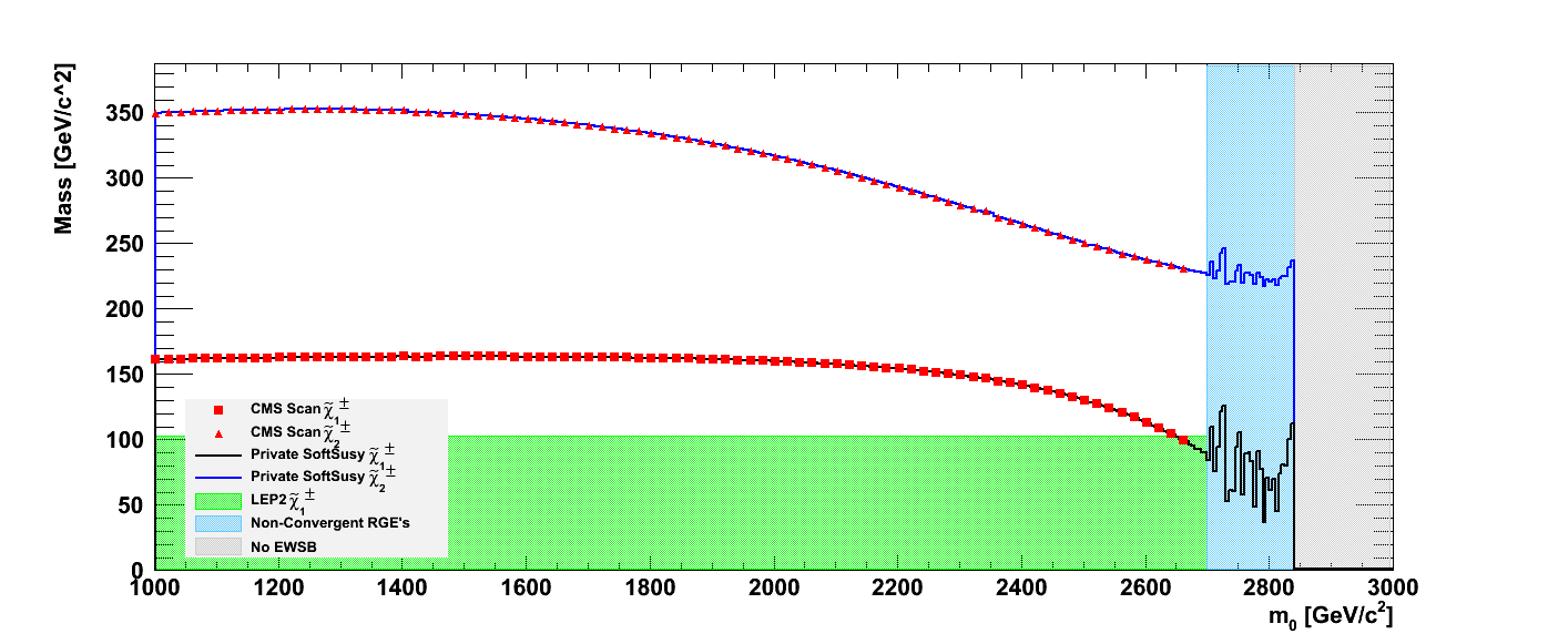
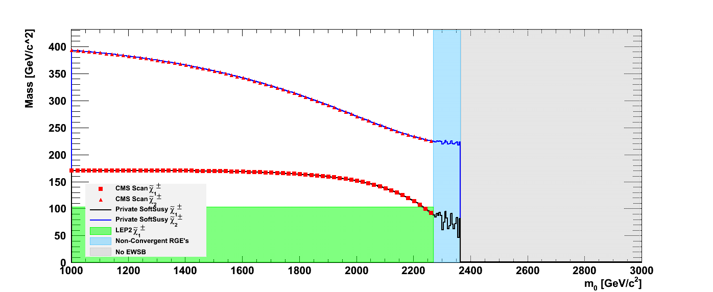
Like all other SUSY spectrum calculators, SoftSusy checks for convergence after each iteration, and eventually terminates after a given fixed number of iterations222We have verified that increasing the maximum number of iterations does not alleviate the convergence problem, i.e. the chaotic behavior is intrinsically present in the system.. One should keep in mind that even though SoftSusy warns the user of the non-convergence problem, it still provides a mass spectrum, albeit an unreliable one. This is illustrated in Figs. 3(a) and 3(b) which show the masses of the two charginos obtained in SoftSusy as a function of for a horizontal slice across the planes of Figs. 1 and 2 at a fixed value of GeV. Here, the region of RGE non-convergence as reported by SoftSusy is shaded in light blue. In this region, the expected value of as calculated from minimizing the radiatively corrected effective potential, is rather small, and the lightest chargino is higgsino-like. The oscillatory behavior of its mass at high is an indication of the convergence problem. Since the value of in the non-convergence region is small, this region is always found to buffer the gray “No EWSB” region in which . It is important to emphasize that non-convergence of the RGEs by itself does not necessarily mean that such points are ruled out or disfavored333Non-convergence of the RGEs means simply that — the mass spectrum calculation is unreliable. In those cases, the SoftSusy manual softsusy recommends using an extrapolation from the neighboring regions where the program did converge. — they may very well represent physically viable models and one should not mistakenly incorporate them into the “No EWSB” region where becomes negative. Those are indeed two separate regions and deserve to be distinguished on the canvas.
In both Figs. 3(a) and 3(b) we observe perfect agreement between the chargino masses as calculated by our private SoftSusy scan (solid lines, 5 GeV granularity) and those calculated by the LHC scan CMSscan (red markers, 20 GeV granularity). While for this slice of GeV, the LHC scans do not extend into the regions where non-convergent RGE’s are reported, it does happen in rare cases (a few out of a thousand) — the LHC scan would sample a point that falls just over the boundary of the region of non-convergence. We have checked that the chargino masses obtained in those cases do coincide with the result that one would obtain by extrapolating from the convergent region, so no ill-effects are expected from this occasional trespassing.
III.2 Experimental Constraints
Results from previous experiments can also be interpreted in the context of the mSUGRA parameter space shown in Figs. 1 and 2.
III.2.1 Chargino mass limits from LEP2
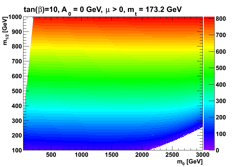
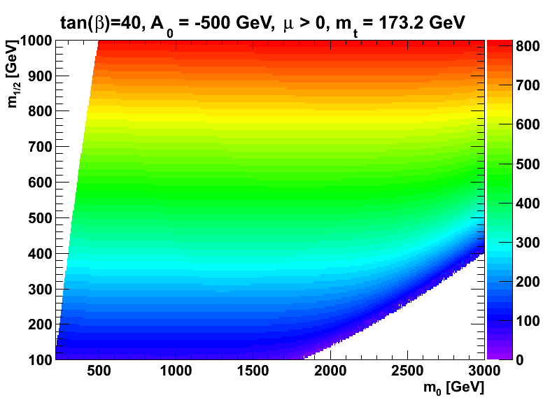
LEP2 searches for chargino pair production are probing the two areas of the plane which exhibit a light chargino (at low , where is wino-like, and at large where becomes small and is higgsino-like). In Figs. 1 and 2 the corresponding regions are colored green and can be understood as excluded at 95% C.L. by LEP2 PDG . For reference, the lightest chargino mass is plotted across the grid in Figs. 4(a) and 4(b) for and , respectively.
III.2.2 Slepton mass limits from LEP2
LEP2 has also performed searches for direct slepton production. Explicitly, the following exclusion limits are imposed PDG :
| (1) | |||||
| (2) | |||||
| (3) |
The relatively small region which satisfies this condition can be found at low and low and is colored yellow in Figs. 1 and 2. It can be understood as excluded at 95% C.L. by LEP2.
III.2.3 Dark matter relic density
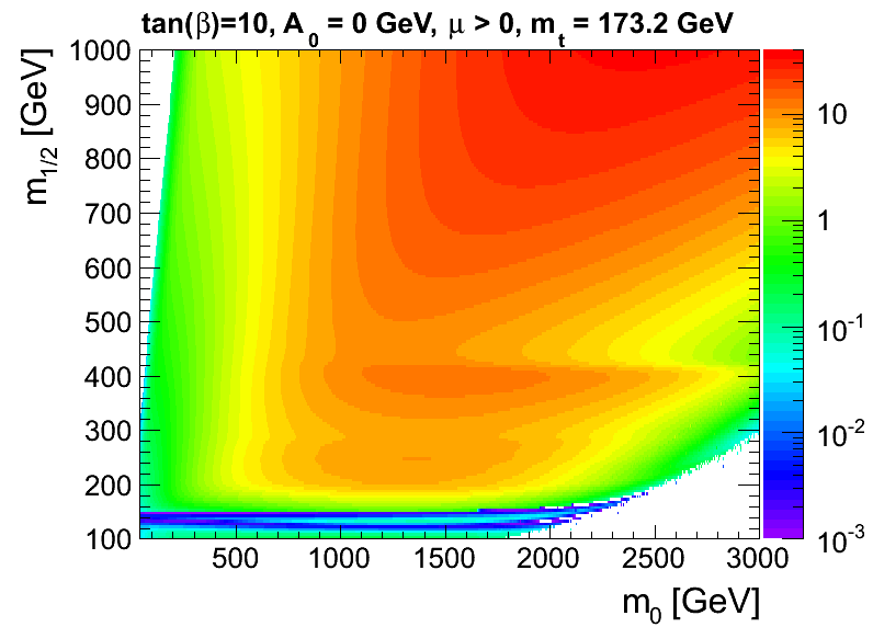
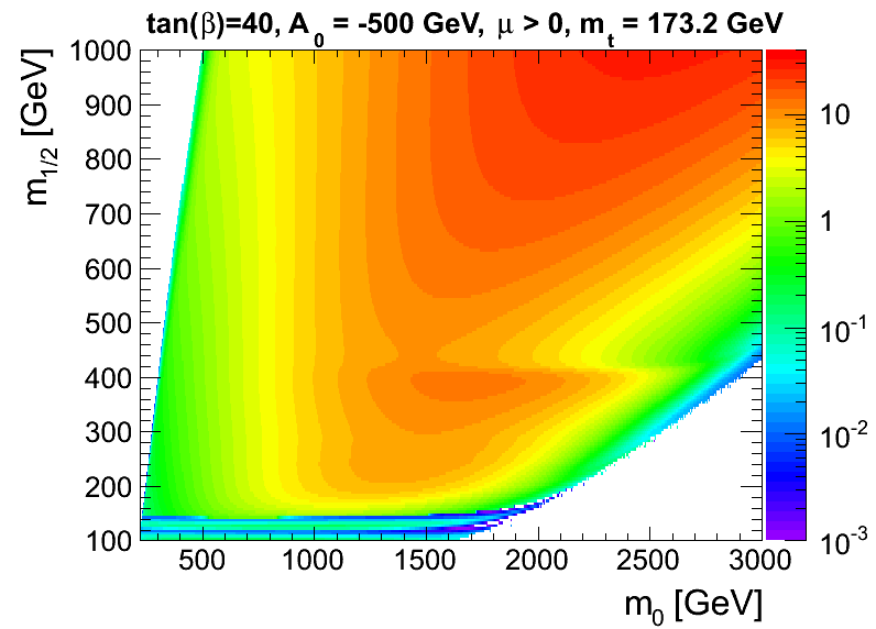
In addition to collider constraints from direct searches for superpartners, one may also wish to consider the cosmological constraint on the dark matter relic density (which is indirect and perhaps more speculative, since it involves certain assumptions about the composition of the dark matter as well as the thermal history of the Universe). We calculate the neutralino relic density across the grid with MicrOMEGAs version 2.4 Belanger:2010gh using SoftSusy-3.2.4 for mass spectrum calculations. The resulting is displayed in Figs. 5(a) and 5(b) for and , respectively. One can see that throughout most of the parameter space, the neutralino relic density is quite larger than the WMAP preferred range Komatsu:2010fb
| (4) |
Model points satisfying eq. (4) yield the appropriate amount of dark matter to within 3 of the measured value of 0.1123 0.0035 and are denoted by magenta filled circles in version 2 of the templates on Figs. 1(b) and 2(b). As expected, the proper relic density is obtained in two areas: 1) the neutralino-stau coannihilation region Ellis:1998kh near the boundary of the “ LSP” region and 2) the “focus-point” region at large Feng:1999mn ; Feng:1999zg ; Chan:1997bi , where the neutralino LSP picks up a non-negligible higgsino component Feng:2000gh . Other notable features on the plot in Fig. 5(a) include the opening of the neutralino annihilation channel into pairs of top quarks (near GeV) and pairs of Higgs and/or gauge bosons (in the neighborhood of GeV).
IV Mass spectrum
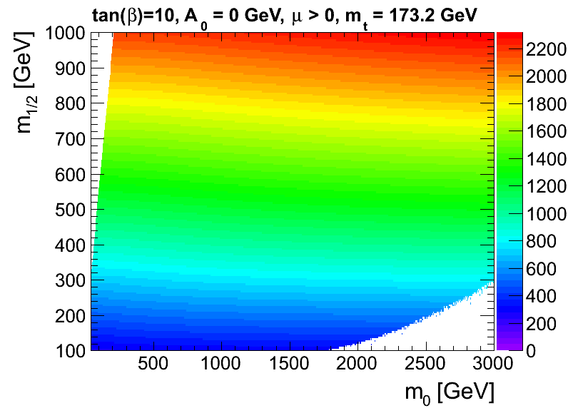
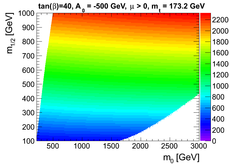
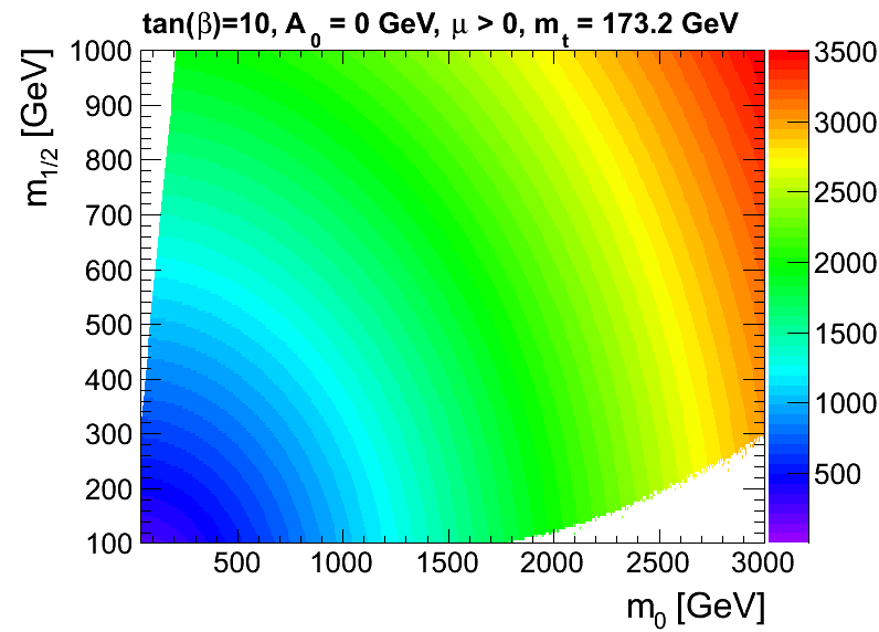
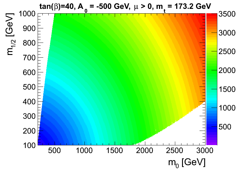
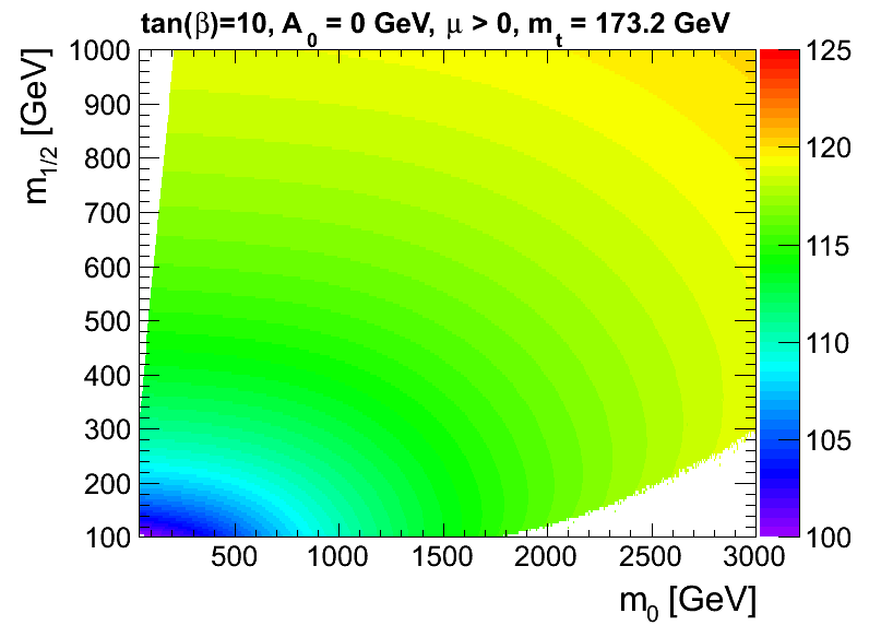
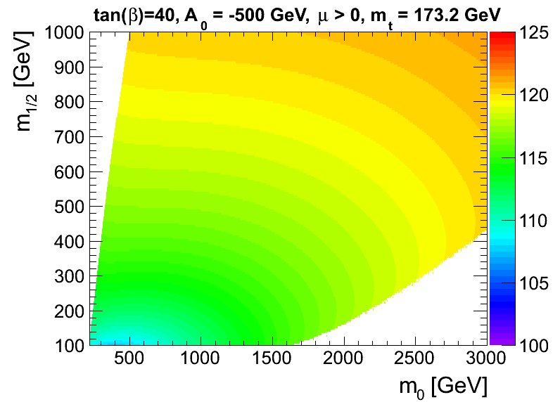
It is a tradition to display a few meaningful isomass contours for particles of interest on the mSUGRA canvas. In the past, the gluino and squark masses were displayed in 250 GeV intervals.444Here we take the average of the four first generation squarks. These are observed to always be within 8% of one another. We continue to display these contours, opting for 500 GeV intervals to reduce congestion. In Version (2) of the templates we go further and provide two additional contours for a Higgs mass of 115 and 120 GeV, respectively. These values are particularly relevant at this stage as the results of the Higgs searches at the LHC may soon make contact with this parameter space Feng:2011aa . As a reference, Figs. 6, 7, and 8 show the masses of the gluino, squark (average), and light CP-even Higgs boson, respectively, across the plane.
V Application
It is expected that Version (1) of the templates is used for public presentation. Both versions, however, are available as TCanvas objects and C-macros in the ROOT framework. These can be downloaded from the web at
-
•
tier2.ihepa.ufl.edu/~remington/SUSY/mSUGRA/GridTanb10_v1.root (.C)
tier2.ihepa.ufl.edu/~remington/SUSY/mSUGRA/GridTanb10_v2.root (.C) -
•
tier2.ihepa.ufl.edu/~remington/SUSY/mSUGRA/GridTanb40_v1.root (.C)
tier2.ihepa.ufl.edu/~remington/SUSY/mSUGRA/GridTanb40_v2.root (.C)
and are also available as ancillary files from the arXiv version of this note.
The following code can be used in ROOT (v.27) to draw the canvas from the root files above:
TFile f(‘‘GridTanb10_v1.root’’); TCanvas *c = (TCanvas*) f.Get(‘‘GridCanvas’’); c->Draw(); MyExclusionContour->Draw(‘‘SAME’’);
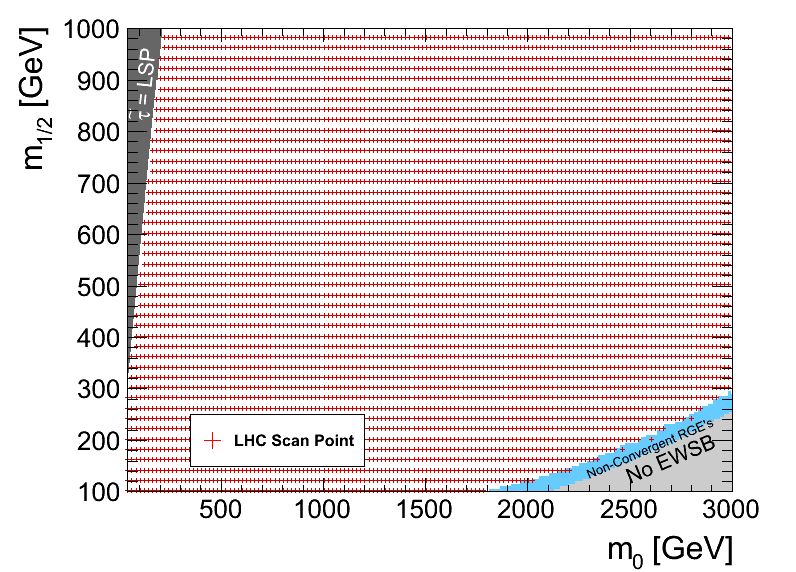
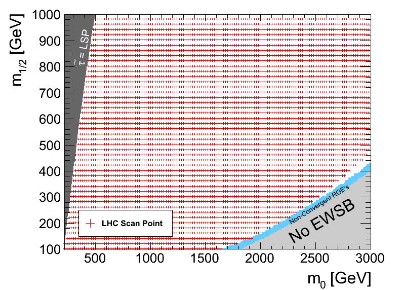
As a final check, we survey the model points that are expected to be in the official LHC scans CMSscan and we represent them symbolically with a “+” on top of our templates to assess the coverage. This can be seen in Figs. 9 and 10 for and , respectively. For we see that there is full coverage everywhere. For , however, we see a small envelope in between the dark matter preferred region and the non-convergent RGE region where the LHC scan does not sample. Our recommendation is that future scans should be extended to include this interesting region. Analysts should be prepared to perform a small extrapolation in this region in the case that their exclusion contour terminates nearby.
Acknowledgments
We thank the CMS SUSY group conveners for encouragement and S. Mrenna and S. Padhi for useful discussions. We also thank J. L. Feng for pointing out some inconsistencies in the previous mSUGRA templates used by CMS and ATLAS.
References
- (1) Y. Golfand and E. Likhtman, “Extension of the Algebra of Poincare Group Generators and Violation of p Invariance,” JETP Lett. 13 (1971) 323–326.
- (2) P. Ramond, “Dual Theory for Free Fermions,” Phys.Rev. D3 (1971) 2415–2418.
- (3) A. Neveu and J. Schwarz, “Factorizable dual model of pions,” Nucl.Phys. B31 (1971) 86–112.
- (4) A. Neveu and J. Schwarz, “Quark Model of Dual Pions,” Phys.Rev. D4 (1971) 1109–1111.
- (5) D. Volkov and V. Akulov, “Is the Neutrino a Goldstone Particle?,” Phys.Lett. B46 (1973) 109–110.
- (6) J. Wess and B. Zumino, “A Lagrangian Model Invariant Under Supergauge Transformations,” Phys.Lett. B49 (1974) 52.
- (7) J. Wess and B. Zumino, “Supergauge Transformations in Four-Dimensions,” Nucl.Phys. B70 (1974) 39–50.
- (8) P. Fayet, “Spontaneously Broken Supersymmetric Theories of Weak, Electromagnetic and Strong Interactions,” Phys.Lett. B69 (1977) 489.
- (9) M. Battaglia, A. De Roeck, J. R. Ellis, F. Gianotti, K. Matchev, et al., “Proposed post-LEP benchmarks for supersymmetry,” Eur.Phys.J. C22 (2001) 535–561, arXiv:hep-ph/0106204 [hep-ph].
- (10) B. Allanach, M. Battaglia, G. Blair, M. S. Carena, A. De Roeck, et al., “The Snowmass points and slopes: Benchmarks for SUSY searches,” Eur.Phys.J. C25 (2002) 113–123, arXiv:hep-ph/0202233 [hep-ph].
- (11) M. Battaglia, A. De Roeck, J. R. Ellis, F. Gianotti, K. Olive, et al., “Updated post - WMAP benchmarks for supersymmetry,” Eur.Phys.J. C33 (2004) 273–296, arXiv:hep-ph/0306219 [hep-ph].
- (12) S. AbdusSalam, B. Allanach, H. Dreiner, J. Ellis, U. Ellwanger, et al., “Benchmark Models, Planes, Lines and Points for Future SUSY Searches at the LHC,” Eur.Phys.J. C71 (2011) 1835, arXiv:1109.3859 [hep-ph].
- (13) B. Allanach, M. Bernhardt, H. Dreiner, C. Kom, and P. Richardson, “Mass Spectrum in R-Parity Violating mSUGRA and Benchmark Points,” Phys.Rev. D75 (2007) 035002, arXiv:hep-ph/0609263 [hep-ph].
- (14) A. H. Chamseddine, R. L. Arnowitt, and P. Nath, “Locally Supersymmetric Grand Unification,” Phys.Rev.Lett. 49 (1982) 970.
- (15) R. Barbieri, S. Ferrara, and C. A. Savoy, “Gauge Models with Spontaneously Broken Local Supersymmetry,” Phys.Lett. B119 (1982) 343.
- (16) L. J. Hall, J. D. Lykken, and S. Weinberg, “Supergravity as the Messenger of Supersymmetry Breaking,” Phys.Rev. D27 (1983) 2359–2378.
- (17) B. Allanach, S. Kraml, and W. Porod, “Theoretical uncertainties in sparticle mass predictions from computational tools,” JHEP 0303 (2003) 016, arXiv:hep-ph/0302102 [hep-ph].
- (18) B. C. Allanach, “Softsusy: A program for calculating supersymmetric spectra,” Computer Physics Communications 143 no. 3, (2002) 305 – 331.
- (19) H. Baer, C.-H. Chen, R. B. Munroe, F. E. Paige, and X. Tata, “Multichannel search for minimal supergravity at and colliders,” Phys.Rev. D51 (1995) 1046–1050, arXiv:hep-ph/9408265 [hep-ph].
-
(20)
The SLHA files for the official CMS mSUGRA scans can be downloaded from
http://cmssw.cvs.cern.ch/cgi-bin/cmssw.cgi/UserCode/SusyAnalysis/SLHAFILES/mSugraScan/. - (21) J. L. Feng, A. Rajaraman, and F. Takayama, “Superweakly interacting massive particles,” Phys.Rev.Lett. 91 (2003) 011302, arXiv:hep-ph/0302215 [hep-ph].
- (22) J. L. Feng, A. Rajaraman, and B. T. Smith, “Minimal supergravity with ,” Phys.Rev. D74 (2006) 015013, arXiv:hep-ph/0512172 [hep-ph].
- (23) A. Djouadi, J.-L. Kneur, and G. Moultaka, “SuSpect: A Fortran code for the supersymmetric and Higgs particle spectrum in the MSSM,” Comput.Phys.Commun. 176 (2007) 426–455, arXiv:hep-ph/0211331 [hep-ph].
- (24) W. Porod, “SPheno, a program for calculating supersymmetric spectra, SUSY particle decays and SUSY particle production at e+ e- colliders,” Comput.Phys.Commun. 153 (2003) 275–315, arXiv:hep-ph/0301101 [hep-ph].
- (25) F. E. Paige, S. D. Protopopescu, H. Baer, and X. Tata, “ISAJET 7.69: A Monte Carlo event generator for pp, anti-p p, and e+e- reactions,” arXiv:hep-ph/0312045 [hep-ph].
- (26) K. Nakamura et al., “Review of particle physics,” Journal of Physics G: Nuclear and Particle Physics 37 no. 7A, (2010) 075021. http://pdg.lbl.gov.
- (27) G. Belanger et al., “Indirect search for dark matter with micrOMEGAs2.4,” Comput. Phys. Commun. 182 (2011) 842–856, arXiv:1004.1092 [hep-ph].
- (28) WMAP Collaboration Collaboration, E. Komatsu et al., “Seven-Year Wilkinson Microwave Anisotropy Probe (WMAP) Observations: Cosmological Interpretation,” Astrophys.J.Suppl. 192 (2011) 18, arXiv:1001.4538 [astro-ph.CO].
- (29) J. R. Ellis, T. Falk, and K. A. Olive, “Neutralino - Stau coannihilation and the cosmological upper limit on the mass of the lightest supersymmetric particle,” Phys.Lett. B444 (1998) 367–372, arXiv:hep-ph/9810360 [hep-ph].
- (30) J. L. Feng, K. T. Matchev, and T. Moroi, “Multi - TeV scalars are natural in minimal supergravity,” Phys.Rev.Lett. 84 (2000) 2322–2325, arXiv:hep-ph/9908309 [hep-ph].
- (31) J. L. Feng, K. T. Matchev, and T. Moroi, “Focus points and naturalness in supersymmetry,” Phys.Rev. D61 (2000) 075005, arXiv:hep-ph/9909334 [hep-ph].
- (32) K. L. Chan, U. Chattopadhyay, and P. Nath, “Naturalness, weak scale supersymmetry and the prospect for the observation of supersymmetry at the Tevatron and at the CERN LHC,” Phys.Rev. D58 (1998) 096004, arXiv:hep-ph/9710473 [hep-ph].
- (33) J. L. Feng, K. T. Matchev, and F. Wilczek, “Neutralino dark matter in focus point supersymmetry,” Phys.Lett. B482 (2000) 388–399, arXiv:hep-ph/0004043 [hep-ph].
- (34) J. L. Feng, K. T. Matchev, and D. Sanford, “Focus Point Supersymmetry Redux,” arXiv:1112.3021 [hep-ph].