A combined first and second order variational approach for image reconstruction
Abstract.
In this paper we study a variational problem in the space of functions of bounded Hessian. Our model constitutes a straightforward higher-order extension of the well known ROF functional (total variation minimisation) to which we add a non-smooth second order regulariser. It combines convex functions of the total variation and the total variation of the first derivatives. In what follows, we prove existence and uniqueness of minimisers of the combined model and present the numerical solution of the corresponding discretised problem by employing the split Bregman method. The paper is furnished with applications of our model to image denoising, deblurring as well as image inpainting. The obtained numerical results are compared with results obtained from total generalised variation (TGV), infimal convolution and Euler’s elastica, three other state of the art higher-order models. The numerical discussion confirms that the proposed higher-order model competes with models of its kind in avoiding the creation of undesirable artifacts and blocky-like structures in the reconstructed images – a known disadvantage of the ROF model – while being simple and efficiently numerically solvable.
1. Introduction
We consider the following general framework of a combined first and second order non-smooth regularisation procedure. For a given datum , , , we compute a regularised reconstruction as a minimiser of a combined first and second order functional . More precisely, we are interested in solving
| (1.1) |
for , non-negative regularisation parameters , convex functions , with at most linear growth at infinity, and a suitable linear operator , see Section 3 for details. The appropriate space for this minimisation is the space of functions of bounded Hessian which consists of all functions such that is a function of bounded variation. The idea of this combination of first and second order dynamics is to regularise with a fairly large weight in the first order term – preserving the jumps as good as possible – and using a not too large weight for the second order term such that artifacts (staircasing) created by the first order regulariser are eliminated without introducing any serious blur in the reconstructed image. We will show that for image denoising, deblurring as well as inpainting the model (1.1) offers solutions whose quality (accessed by an image quality measure) is not far off from the ones produced by some of the currently best higher-order reconstruction methods in the field, e.g., the recently proposed total generalised variation (TGV) model [14]. Moreover, the computational effort needed for its numerical solution is not much more than the one needed for solving the standard ROF model [61]. For comparison the numerical solution for TGV regularisation is in general about ten times slower than this, see Table 1 at the end of the paper.
In this paper we prove existence and uniqueness of (1.1) for the classical setting of the problem in the space by means of relaxation. The generality of this result includes both the classical variational formulation in , e.g. for the Huber regularised version of the total variation, as well as the non-smooth norm minimisation setting in , which constitutes the relaxed version of (1.1). In the numerical part of the paper a discretised version of (1.1) is minimised by means of an operator splitting technique for the cases and , and its application to image denoising, deblurring and inpainting is discussed.
The rest of the introduction is structured as follows. In Section 1.1 we phrase the general inverse problem for image reconstruction, which leads us to non-smooth norm minimisation, e.g. total variation minimisation, and eventually to the introduction of higher-order regularisers within this class. This section is followed by a presentation of state of the art higher-order methods in imaging in Section 1.2 and a discussion of some models from this group which are closely related to (1.1) in Section 1.3.
1.1. Context
A general inverse problem in imaging reads as follows. Observing or measuring data in a suitable Hilbert space of real functions defined on a domain , we seek for the original or reconstructed image that fulfils the model
| (1.2) |
where is a linear operator in , i.e., , and denotes a possible noise component which – depending on the noise statistics – might depend on the data . The operator is the forward operator of this problem. Examples are blurring operators (in which case denotes the convolution of with a blurring kernel), the Fourier transform or a projection operator onto a subspace of (i.e., only a few samples of are given).
To reconstruct one has to invert the operator . This is not always possible since in many applications a problem can be ill-posed and further complicated by interferences like noise. In this case a common procedure in inverse problems is to add a-priori information to the model, which in general is given by a certain regularity assumption on the image . Hence, instead of solving (1.2) one computes as a minimiser of
defined in a suitable Banach space . Here, models the regularity assumption on with a certain regularity parameter and is called the regulariser of the problem, and is a distance function in that enforces (1.2). The latter depends on the statistics of the data , which can be either estimated or are known from the physics behind the acquisition of . For corrupted by normally distributed additive noise, this distance function is the squared norm of . For the choice of the regulariser , squared Hilbert space norms have a long tradition in inverse problems. The most prominent example is regularisation
| (1.3) |
see also [68, 75]. For , the gradient flow of the corresponding Euler-Lagrange equation of (1.3) reads . The result of such a regularisation technique is a linearly, i.e., isotropically, smoothed image , for which the smoothing strength does not depend on . Hence, while eliminating the disruptive noise in the given data also prominent structures like edges in the reconstructed image are blurred. This observation gave way to a new class of non-smooth norm regularisers, which aim to eliminate noise and smooth the image in homogeneous areas, while preserving the relevant structures such as object boundaries and edges. More precisely, instead of (1.3) one considers the following functional over the space :
| (1.4) |
where is a function from to with at most linear growth, see [70]. As stated in (1.4) the minimisation of over is not well-posed in general. For this reason relaxation procedures are applied, which embed the optimisation for into the optimisation for its lower semicontinuous envelope within the larger space of functions of bounded variation, see Section 2. The most famous example in image processing is , which for results in the so-called ROF model [61]. In this case the relaxed formulation of (1.4) is the total variation denoising model, where is replaced by the total variation and is minimised over the space of functions of bounded variation. Other examples for are regularised versions of the total variation like for a positive [1, 41], the Huber-regulariser and alike [28, 47, 22, 54]. The consideration of such regularised versions of is sometimes of advantage in applications where perfect edges are traded against a certain smoothness in homogeneous parts of the image, [58]. Moreover such regularisations become necessary for the numerical solution of (1.4) by means of time-stepping [70] or multigrid-methods [71, 43, 69] for instance.
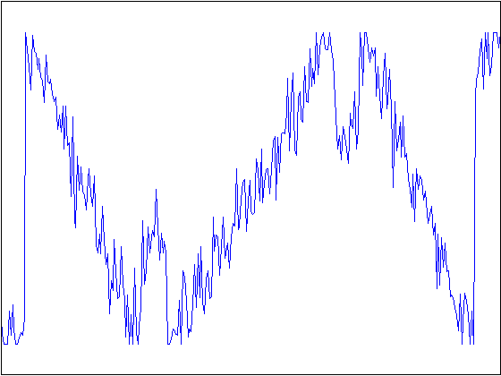
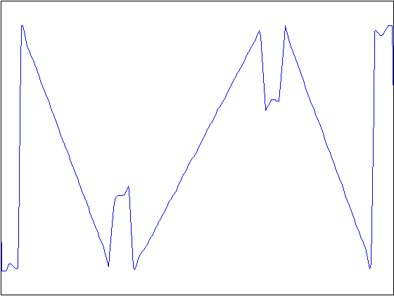
As these and many more contributions in the image processing community have proven, this new non-smooth regularisation procedure indeed results in a nonlinear smoothing of the image, smoothing more in homogeneous areas of the image domain and preserving characteristic structures such as edges. In particular, the total variation regulariser is tuned towards the preservation of edges and performs very well if the reconstructed image is piecewise constant. The drawback of such a regularisation procedure becomes apparent as soon as one considers images or signals (in 1D) which do not only consist of flat regions and jumps, but also possess slanted regions, i.e., piecewise linear parts. The artifact introduced by total variation regularisation in this case is called staircasing. Roughly this means that the total variation regularisation of a noisy linear function in one dimension is a staircase , whose norm is close to , see Figure 1. In two dimensions this effect results in blocky-like images, see Figure 2. In one dimension this effect has been rigorously studied in [31].
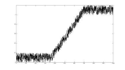
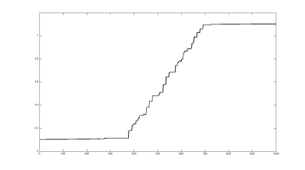
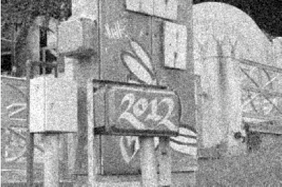


One way to reduce this staircasing effect is in fact to “round off” the total variation term by using regularised versions defined by functions as indicated above, e.g., Huber regularisation [58]. However, such a procedure can only reduce these artifacts to a certain extent. For instance, the Huber-type regularisation will eliminate the staircasing effect only in areas with small gradient. Another way of improving total variation minimisation is the introduction of higher-order derivatives in the regulariser as in (1.1). Especially in recent years, higher-order versions of non-smooth image enhancing methods have been considered.
1.2. Related work
Already in the pioneering paper of Chambolle and Lions [22] the authors propose a higher-order method by means of an inf-convolution of two convex regularisers. Here, a noisy image is decomposed into three parts by solving
| (1.5) |
where is the distributional Hessian of . Then, is the piecewise constant part of , the piecewise smooth part and the noise (or texture). Along these lines a modified infimal-convolution approach has been recently proposed in the discrete setting in [65, 66]. Another attempt to combine first and second order regularisation originates from Chan, Marquina, and Mulet [26], who consider total variation minimisation together with weighted versions of the Laplacian. More precisely, they consider a regularising term of the form
where must be a function with certain growth conditions at infinity in order to allow jumps. The well-posedness of the latter in one space dimension has been rigorously analysed by Dal Maso, Fonseca, Leoni and Morini [31] via the method of relaxation.
The idea of bounded Hessian regularisers was also considered by Lysaker et al. [52, 53], Chan et al. [27], Scherzer et al. [62, 48], Lai at al. [50] and Bergounioux and Piffet [8]. In these works the considered model has the general form
In Lefkimmiatis et al. [51], the spectral norm of the Hessian matrix is considered. Further, in [60] minimisers of functionals which are regularised by the total variation of the st derivative, i.e.,
are studied. Another interesting higher-order total variation model is proposed by Bredies et al. [14]. The considered regulariser is called total generalised variation (TGV) and is of the form
| (1.6) |
where denotes the space of symmetric tensors of order with arguments in , and are fixed positive parameters. Its formulation for the solution of general inverse problems was given in [13, 16].
Properties of higher-order regularisers in the discrete setting in terms of diffusion filters are further studied in [34]. Therein, the authors consider the Euler-Lagrange equations corresponding to minimisers of functionals of the general type
| (1.7) |
for different non-quadratic penaliser functions . Moreover, Bertozzi and Greer [10] have rigorously studied the fourth-order evolution equation which arises as a gradient flow of , where is a nondecreasing function of quadratic growth in a neighbourhood of and at most linear growth at infinity. Solutions of this model are called low curvature image simplifiers and are given by
when .
Higher-order inpainting methods in general perform much better than first order methods – like total variation inpainting – because of the additional directional information used for the interpolation process. Euler’s elastica is a popular higher-order variational method [25, 67]. There, the regularising term reads:
i.e., is a combination of the total variation and the curvature of the level lines of (a nonlinear second order regularising term). Other examples of higher-order inpainting are the Cahn-Hilliard inpainting [9], TV-H-1 inpainting [17, 63] and Hessian-based surface restoration [50].
1.3. Relation of our model to TGV, infimal convolution regularisation, higher-order diffusion filters and Euler’s elastica
In this section we want to analyse the connection of our combined first and second order approach (1.1) with infimal convolution (1.5) [22, 65, 66], the total generalised variation regulariser of order two (1.6) [14] and with higher-order diffusion filters [34]. Moreover, in the case of inpainting, we discuss the connection of our model to Euler’s elastica [25, 67].
In the case of inf-convolution (1.5) the regularised image consists of a function and a function which are balanced against each other by positive parameters . Differently, a minimiser of (1.1) is in as a whole and as such is more regular than the infimal convolution minimiser which is a function in . Hence, infimal convolution reproduces edges in an image as perfect jumps while in our combined first and second order total variation approach edges are lines where the image function has a large but finite gradient everywhere. We believe that our approach (1.1) can be made equivalent to infimal convolution if combined with the correct choice of adaptive regularisation, e.g. [35, 42]. More precisely, we replace the two constant parameters and by spatially varying functions and minimise for
Then, we can choose and according to (1.5), i.e., where , where , and correctly balancing and in the rest of . However, let us emphasise once more that this is not our intention here.
The relation of (1.1) to the regularisation approach with total generalised variation [14] of order can be understood through its equivalence with the modified infimal convolution approach [66] in the discrete setting. The total generalised variation of order is defined for a positive multi-index as
where is the space of symmetric tensors of order with arguments in . An alternative definition of TGV was proven in [16]
where BD is the space of functions of bounded deformation, is the distributional symmetrised gradient of and denotes the total variation measure evaluated on .
The relation to higher-order diffusion filters as analysed in [34] becomes apparent when considering the Euler-Lagrange equation of (1.1) in the case and , having the form , , where is convex and has at most linear growth. Namely, with appropriate boundary conditions we obtain the following Euler-Lagrange equation
This simplifies for the case to a regularised first-second order total variation reaction-diffusion equation that reads
The consideration of the corresponding evolution equations for (1.3) in the presence of different choices of penalising functions promises to give rise to additional properties of this regularisation technique and is a matter of future research.
As far as inpainting is concerned, we examine here the connection of our method to Euler’s elastica. Depending on how each of the terms in the Euler’s elastica regulariser are weighted, the interpolation process is performed differently. If a larger weight is put on the total variation the interpolation results into an image with sharp edges, which however can get disconnected if the scale of the gap is larger than the scale of the object whose edges should be propagated into it. This behaviour is a validation of the so-called “good continuation principle” defined by the Gestaltist school [49] and not desirable in image inpainting. Putting a larger weight on the curvature term however resolves this issue and gives satisfying results with respect to the continuation principle. The right combination (balance) of these two terms seems to result into a good tradeoff between “sharpness” and “continuation” of edges. However, one disadvantage of the Euler’s elastica inpainting model for analytic and numerical issues is that it is a non-convex minimisation problem. In particular, numerical algorithms are in general not guaranteed to converge to a global minimiser, only local minimisation can be achieved. The minimisation of functional (1.1) can be seen as a convex simplification of the Euler’s elastica idea, where we have replaced the non-convex curvature by the convex total variation of the first derivative of .
For more discussion and comparison of higher-order regularisers we recommend Chapters 4.1.5-4.1.7 and 6.4 in [5].
Outline of the paper: In Section 2 we give a brief introduction to Radon measures, convex functions of measures and functions of bounded variation. In Section 3 we introduce the variational problem (1.1) and the space that this functional is naturally defined in. We define two topologies on and we identify the lower semicontinuous envelope of (1.1) with respect to these topologies. Finally, we prove the well-posedness – existence, uniqueness, stability – of the minimisation of the relaxed functional using standard techniques from calculus of variations and Bregman distances. Section 4 deals with two special versions of (1.1), the anisotropic version and the case with the norm in the fidelity term. In Section 5 we introduce the corresponding discretised problem and we propose the split Bregman method for its numerical implementation in the case , . In Sections 6, 7 and 8 we present some numerical examples of our method in image denoising, deblurring and inpainting respectively. Finally, in Section 9 we discuss how our approach compares with other higher-order methods like infimal convolution (denoising, deblurring), total generalised variation (denoising, deblurring) and Euler’s elastica (inpainting).
2. Preliminaries
In this section, we introduce some basic notions that we are going to use. A reader familiar with Radon measures, functions and relaxed functionals can quickly go through Sections 2.1, 2.3 and 2.4 respectively. Section 2.2 familiarises the reader with convex functions of measures, a perhaps less known subject.
Remarks on standard notation: As usual, we denote with the Lebesgue measure. Different notions are denoted by : When it is applied on vectors or matrices it denotes the Euclidean norm (vector) or the Frobenius norm (matrices). When it is applied on measures it denotes the total variation measure while when it is applied on Borel subsets of it denotes the Lebesgue measure of that subset. Finally, denotes the norm in and denotes the standard Euclidean inner product.
2.1. Finite Radon measures
All our notation and definitions are consistent with [4]. From now on, denotes an open set in . We define the space to be the space of -valued finite Radon measures. The total variation measure of is denoted by . We say that a sequence in converges weakly∗ to a measure and we write if for all , the completion of endowed with the supremum norm. Thus converges weakly∗ to if it converges weakly∗ component-wise. We will often consider the Lebesgue decomposition of a -valued finite Radon measure with respect to a -finite positive Borel measure :
where is the absolutely continuous part of with respect to , is the singular part and denotes the density function of with respect to (Radon-Nikodým derivative). Again this is nothing else than the usual Lebesgue decomposition regarded component-wise. Recall also that any is absolutely continuous with respect to its total variation measure and thus we obtain the polar decomposition of
2.2. Convex functions of measures
Let be a continuous function from to which is positively homogeneous of degree , i.e., for every
Given a measure , we define the -valued measure as follows:
It can be proved that if is a convex function then is a convex function in and if is any positive measure such that is absolutely continuous with respect to then
We refer the reader to Proposition A.1 in Appendix A for a proof of the above statement. Suppose now that is not necessarily positively homogeneous but it is a continuous function from which is convex and has at most linear growth at infinity, i.e., there exists a positive constant such that
In that case the recession function of is well defined everywhere, where
It can be proved that is a convex function and positively homogeneous of degree . Given a measure we consider the Lebesgue decomposition with respect to Lebesgue measure , and we define the -valued measure as follows:
| (2.1) | |||||
We refer the reader to Theorem A.2 in Appendix A for a result regarding lower semicontinuity of convex functions of measures with respect to the weak∗ convergence.
2.3. The space
We recall that a function is said to be a function of bounded variation or else if its distributional derivative can be represented by a -valued finite Radon measure, which is denoted by . This means that
for some -valued finite Radon measure . The absolutely continuous part of with respect to Lebesgue measure is denoted by . It is immediate that since if then . Consistently, we say that a function belongs to if
In that case is an matrix-valued measure. A function u belongs to if and only if its variation in , is finite, where,
Moreover if then and if , then , where . The space endowed with the norm is a Banach space. It can be shown that if , then is equal to a constant a.e. in any connected component of .
Suppose that , belong to . We say that the sequence converges to weakly∗ in if it converges to in and the sequence of measures converges weakly∗ to the measure . It is known that converges to weakly∗ in if and only if is bounded in and converges to in . The usefulness of the introduction of the weak∗ convergence is revealed in the following compactness result: Suppose that the sequence is bounded in , where is a bounded open set of with Lipschitz boundary. Then there exists a subsequence and a function such that converges to weakly∗ in .
We say that the sequence converges to strictly in if it converges to in and converges to . It is immediate that strict convergence implies weak∗ convergence.
Suppose that is bounded with Lipschitz boundary. Define when and when . Then with continuous embedding. Moreover if is connected then the following inequality holds (Poincaré-Wirtinger):
where the constant depends only on and denotes the mean value of in :
We refer the reader to [4] for a detailed description of the above as well as for an introduction to weak continuity and differentiability notions in and the decomposition of the distributional derivative of a function .
2.4. Relaxed functionals
Suppose that is a set endowed with some topology and let . The relaxed functional or otherwise called the lower semicontinuous envelope of with respect to the topology is a functional defined as follows for every :
It is easy to check that is the greatest lower semicontinuous functional which is smaller or equal than . It can be also checked that
where denotes the open neighbourhoods of . Moreover, if is a first countable topological space, then is characterised by the two following properties:
-
(i)
For every sequence converging to , we have
-
(ii)
There exists a sequence converging to such that
An interesting property of the relaxed functional is that if it has a minimum point then the value of at that point will be equal with the infimum of , i.e.,
For more information on relaxed functionals see [12] and [30].
3. The variational formulation
In the current section we specify our definition of the functional (1.1) that we want to minimise. We start by defining the minimisation problem in the space as this is the space in which our analysis subsumes various choices for the regularisers and . As this space is not reflexive, and thus existence of minimisers cannot be guaranteed, we extend the definition to a larger space. We introduce this larger space as the subspace of all such that . We define the weak∗ and the strict topology of and we identify the lower semicontinuous envelope (relaxed functional) of the extended functional with respect to these topologies. We prove existence of minimisers of the relaxed functional, uniqueness under some assumptions as well as stability.
In the following denotes as usual a bounded, connected, open subset of with Lipschitz boundary, denotes a bounded linear operator from to , and , are non-negative constants. Further we suppose that , are convex functions with at most linear growth at infinity, i.e., there exist positive constants and such that
| (3.1) | |||
| (3.2) |
Moreover, we assume that both and are minimised in and they satisfy a coercivity condition:
| (3.3) | |||
| (3.4) |
where and are strictly positive. We want to minimise the following functional:
| (3.5) |
The natural space for the functional to be defined in, is . Since this space is not reflexive a solution of the minimisation problem by the direct method of calculus of variations does not work. Rather, existence of a minimiser of (3.5) can be shown via relaxation that is: We extend the functional into a larger space which has some useful compactness properties with respect to some topology and we identify the relaxed functional with respect to the same topology. This space is .
3.1. The space
The space (often denoted with ) is the space of functions of bounded Hessian. It was introduced by Demengel in [32] and consists of all functions whose distributional Hessian can be represented by an -valued finite Radon measure. In other words:
We set . Again it is immediate that . is a Banach space equipped with the norm . If has a Lipschitz boundary and it is connected then it can be shown that there exist positive constants and such that
| (3.6) |
Moreover, the embedding from into is compact, see [32]. We denote the approximate differential of with , see [4] for a definition.
Analogously with we define the following notions of convergence in :
Definition 3.1 (Weak∗ convergence in ).
Let belong to . We say that converges to weakly∗ in if
and
or in other words
It is not hard to check that a basis for that topology consists of the following sets:
where , is finite, and . This topology is also metrizable, hence first countable. We do not imply here that is the dual space of a Banach space but we name this convergence to show the correspondence with the weak∗ convergence in . We have also the corresponding compactness result:
Theorem 3.2 (Compactness in ).
Suppose that the sequence is bounded in . Then there exists a subsequence and a function such that converges to weakly∗ in .
Proof.
From the compact embedding of into and the fact that the sequence is bounded in we have that there exists a subsequence , a function and a function such that converges to in and converges to weakly∗ in , as goes to infinity. Then, , and converges to weakly∗ in . ∎
Definition 3.3 (Strict convergence in ).
Let and belong to . We say that converges to strictly in if
and
It is easily checked that the function
is a metric and induces the strict convergence in . The following Lemma can be used to compare these two topologies.
Lemma 3.4.
Suppose that , belong to and converges to strictly in . Then
Proof.
We recall from (3.6) that there exist positive constants and such that
Since the sequence is strictly convergent in , the sequences and are bounded. Hence, there exists a positive constant such that
which implies that the sequence is bounded in . From the compact embedding of into we get that there exists a subsequence and a function such that converges to in . In particular converges to in so and thus converges to in . Since every subsequence of is bounded in we can repeat the same argument and deduce that for every subsequence of there exists a further subsequence which converges to in . This proves that the initial sequence converges to in . ∎
Corollary 3.5.
Strict convergence implies weak∗ convergence in .
3.2. Relaxation of the second order functional
We now extend the functional in (3.5) to in the following way:
| (3.7) |
As we have discussed above, the weak∗ topology in provides a good compactness property which is inherited from the weak∗ topology in . However, the functional is not sequentially lower semicontinuous with respect to the strict topology in and hence it is neither with respect to the weak∗ topology in . Indeed, we can find a function , see [32] for such an example. Hence, from the definition of we have . However, according to Theorem A.3 we can find a sequence in which converges strictly to . It follows that the sequences , as well as are bounded. Moreover the sequence is bounded in . Since is a bounded linear operator and from the fact that and have at most linear growth at infinity we deduce that the sequence is bounded as well. Hence we get
which proves that is not lower semicontinuous with respect to the strict topology in . Thus, we have to identify its lower semicontinuous envelope with respect to the strict convergence. We define the following functional in :
where , the approximate differential of , is also the density of with respect to the Lebesgue measure, see [4]. It is immediate to see that if then . Thus is general, is smaller than .
Theorem 3.6.
The functional is lower semicontinuous with respect to the strict topology in .
Proof.
It is not hard to check that since is convex and has at most linear growth then it is Lipschitz, say with constant . Let and be functions in and let converge to strictly in and thus also weakly∗ in . We have to show that
From the definition of the weak∗ convergence in we have that converges to in . From the Sobolev inequality, see [40],
we have that converges to in . Since is continuous then the map is continuous and hence we have that
| (3.8) |
Moreover since converges to as , we have from the Lipschitz property
i.e., we have
| (3.9) |
Finally we have that weakly∗. We can apply Theorem A.2 for , , and get that
| (3.10) |
From (3.8), (3.9) and (3.10) we get that
∎
Theorem 3.7.
The functional is the lower semicontinuous envelope of with respect to the strict convergence in .
Proof.
Suppose that converges to strictly in . From the lower semicontinuity of we have that and since we get that . For the other direction Theorem A.3 tells us that given there exist a sequence such that converges to strictly in and
| (3.11) |
We have also that converges to in which implies that
| (3.12) | |||
as the proof of Theorem 3.6 shows. From (3.11) and (3.2) we get that
∎
Observe that is also the lower semicontinuous envelope of with respect to the weak∗ convergence in .
Let us note here that in fact the relaxation result of Theorem 3.7 follows from a more general relaxation result in [3]. There, the authors solely assume to be quasi-convex. However, since we consider convex functions the proof we give in this paper is simpler and more accessible to the non-specialist reader.
The proof of the following minimisation theorem follows the proof of the corresponding theorem in [70] for the analogue first order functional. Here we denote with the characteristic function of , i.e., , for all and 0 otherwise.
Theorem 3.8.
Assuming , , then the minimisation problem
| (3.13) |
has a solution .
Proof.
Let be a minimising sequence for (3.13) and let be an upper bound for . We have that
| (3.14) |
for every . From the coercivity assumptions (3.3)-(3.4) and from (3.14) we have
| (3.15) |
for a possibly different constant . We show that the sequence is bounded in , following essentially [70]. By the Poincaré-Wirtinger inequality there exists a positive constant such that for every
Thus it suffices to bound uniformly in . We have for every
It follows that
and thus
since .
Since the sequence is bounded in and is bounded, we have that the sequence is bounded in and moreover it is bounded in . From Theorem 3.2 we obtain the existence of a subsequence and such that converges to weakly∗ in . Since the functional is lower semicontinuous with respect to this convergence we have:
which implies that
∎
Let us note here that in the above proof we needed , in order to get an a priori bound in the norm of the gradient (for see [70]). However, the proof goes through if and is injective. If is not injective and it is not straightforward how to get existence. The proof of the following theorem also follows the proof of the corresponding theorem for the first order analogue in [70].
Proposition 3.9.
If, in addition to , is injective or if is strictly convex, then the solution of the minimisation problem (3.13) is unique.
Proof.
Using the Proposition A.1 in Appendix A we can check that the functional is convex. Let , be two minimisers. If then from the strict convexity of the first term of we have
which is a contradiction. Hence and if is injective we have . If is not injective but is strictly convex then we must have otherwise we get the same contradiction as before. In that case, since is connected, there exists a constant such that and since , we get . ∎
3.3. Stability
To complete the well-posedness picture for (1.1) it remains to analyse the stability of the method. More precisely, we want to know which effect deviations in the data have on a corresponding minimiser of (1.1). Ideally the deviation in the minimisers for different input data should be bounded by the deviation in the data. Let be the regularising functional in (1.1), i.e.,
It has been demonstrated by many authors [18, 19, 59, 7] that Bregman distances related to the regularisation functional are natural error measures for variational regularisation methods with convex. In particular Pöschl [59] has derived estimates for variational regularisation methods with powers of metrics, which apply to the functional we consider here. However, for demonstration issues and to make constants in the estimates more explicit let us state and prove the result for a special case of (1.1) here.
We consider functional (1.1) for the case . For what we are going to do we assume that one of the regularisers is differentiable. Without loss of generality, we assume that is differentiable in . The analogous analysis can be done if is differentiable or even under weaker, continuity conditions on and , see [15]. Let be the original image and the exact datum (without noise), i.e. is a solution of . We assume that the noisy datum deviates from the exact datum by for a small . For the original image we assume that the following condition, called source condition, holds
| (SC) |
where denotes the domain of the operator and is the subdifferential of . Moreover, since is differentiable and both and are convex, the subdifferential of can be written as the sum of subdifferentials of the two regularisers, i.e.,
see [38][Proposition 5.6., pp. 26]. We define the symmetric Bregman distance for the regularising functional as
Theorem 3.10.
Proof.
Remark 3.11.
In the case we obtain the classical form of Bregman error estimates, that is
4. Special cases and extensions
In this section we introduce two more versions of the functional , the anisotropic version and the version where the norm appears in the fidelity term.
4.1. The anisotropic version
We introduce the anisotropic version of the functional in (3.5). Note that when , then the relaxed functional is given by
Its anisotropic analogue is defined for and . In that case, the relaxed functional is given by
| (4.1) | |||||
where , denotes the distributional derivative with respect to and respectively. Since the functional is obtained for the above choice of and , the following theorem holds as a special case of Theorem 3.8:
Theorem 4.1.
Assuming , the minimisation problem
| (4.2) |
has a solution. If is injective then the solution is unique.
4.2. fidelity term
We consider here the case with the norm in the fidelity term, i.e.,
| (4.3) |
where for simplicity we consider the case , . As it has been shown in [55] and also studied in [24] and [36], the norm in the fidelity term leads to efficient restorations of images that have been corrupted by impulse noise.
Theorem 4.2.
Assuming , the minimisation problem
| (4.4) |
has a solution.
Proof.
The proof is another application of the direct method of calculus of variation. Similarly with the proof of Theorem 3.8 we show that any minimising sequence is bounded in . Hence it is bounded in . Thus we can extract a weakly∗ convergent subsequence in . Trivially, the functional is lower semicontinuous with respect to that convergence. ∎
5. The numerical implementation
In this section we work with the discretised version of the functional (3.5) and we discuss its numerical realisation by the so-called split Bregman technique [46]. We start by defining the discrete versions of and norms in Section 5.1. In Section 5.2 we proceed with an introduction to the Bregman iteration which is used to solve constrained optimisation problems, an idea originated in [56]. In [46] the Bregman iteration and an operator splitting technique (split Bregman) is used in order to solve the total variation minimisation problem. In the latter paper it was also proved that the iterates of the Bregman iteration converge to the solution of the constrained problem assuming that the iterates satisfy the constraint in a finite number of iterations. Here, we give a more general convergence result where we do not use that assumption, see Theorem 5.1. Finally in Section 5.3 we describe how our problem is solved with the Bregman iteration, using the splitting procedure mentioned above.
5.1. The discretised setting
In this section we study the discretisation and minimisation of the functional (3.5). In our numerical examples we consider , and the data fidelity term is measured in the norm, i.e.,
| (5.1) |
In order to discretise (5.1) we specify the corresponding discrete operators and norms that appear in the continuous functional. We denote the discretised version of (5.1) with . In the discrete setting, is an element of and is a bounded linear operator from to . For and , the discrete functional is given by
| (5.2) |
where for every , and we define
For the formulation of the discrete gradient and Hessian operators we use periodic boundary conditions and we follow [76]. We also refer the reader to [57] where the form of the discrete differential operators is described in detail. We define and div consistently with the continuous setting as adjoint operators and the same is done for the Hessian and its adjoint .
In particular the first and second order divergence operators, div and , have the properties:
where the “” denotes the Euclidean inner product, if we consider , and as large vectors formed successively by the columns of the corresponding matrices.
5.2. Constrained optimisation and the Bregman iteration
We now introduce the Bregman and the split Bregman iteration as a numerical method for the solution of (5.2). We would like to recall some basic aspects of the general theory of Bregman iteration before finishing this discussion with the convergence result in Theorem 5.1.
Suppose we have to solve the following constrained minimisation problem:
| (5.3) |
where the function is convex and is a linear map from to . We transform the constrained minimisation problem (5.3) into an unconstrained one, introducing a parameter :
| (5.4) |
where in order to satisfy the constraint we have to let increase to infinity. Instead of doing that we perform the Bregman iteration as it was proposed in [56] and [77]:
Bregman Iteration
| (5.5) | |||||
| (5.6) |
In [56], assuming that (5.5) has a unique solution, the authors derive the following facts for the iterates :
| (5.7) |
| (5.8) |
| (5.9) |
and
| (5.10) |
The following theorem was proved in [46] in the case where the iterates of Bregman iteration satisfy the constraint in a finite number of iterations. In other words, it was proved that if for some iterate we have then is a solution to the original constrained problem (5.3). In the following theorem we give a more general proof where we do not use that assumption, something that makes it a genuine contribution to the convergence theory of Bregman iteration.
Theorem 5.1.
Proof.
We have that the statements (5.7)-(5.10) hold. Moreover, we have for every ,
From (5.10) and the coercivity of we get that the sequence is bounded, say by a constant . Thus, it suffices to show that every accumulation point of is equal to . Since , for every increasing sequence of naturals , we have that
Now because of the fact that
we get that
| (5.11) | |||||
Suppose now that converges to some as goes to infinity. Then taking into account (5.7), also satisfies
| (5.12) |
Taking limits in (5.11) and using Kronecker’s lemma, see Lemma A.4, we have that the limit in the right hand side of (5.11) is . Thus, we have
and since is the solution of the constrained minimisation problem and (5.12) holds, we have . Since every accumulation point of the bounded sequence is equal to , we conclude that the whole sequence converges to . ∎
5.3. Numerical solution of our minimisation problem
In this section, we explain how the Bregman iteration (5.5)-(5.6) together with an operator splitting technique can be used to implement numerically the minimisation of functional (5.2). The idea originates from [46] where such a procedure is applied to total variation minimisation and is given the name split Bregman algorithm. This iterative technique is equivalent to certain instances of combinations of the augmented Lagrangian method with classical operator splitting such as Douglas-Rachford, see [64]. We also refer the reader to the paper of Benning, Brune, Burger and Müller [6], for applications of Bregman methods to higher-order regularisation models for image reconstruction.
Exemplarily, we present the resulting algorithm for the minimisation of J in (5.2), i.e., for , and data fidelity term. Recall that we want to solve the following unconstrained minimisation problem:
| (5.13) |
The derivation of the split Bregman algorithm for solving (5.13) starts with the first observation that the above minimisation problem is equivalent to the following constrained minimisation problem:
| (5.14) |
It is clear that since the gradient and the Hessian are linear operations, the minimisation problem (5.14) can be reformulated into the more general problem:
| (5.15) |
where is convex, is a matrix and is a vector of length .
It is easy to see that the iterative scheme of the type (5.5)-(5.6) that corresponds to the constraint minimisation problem (5.14) is :
| (5.17) | |||||
| (5.18) |
where and .
Remark 5.2.
Our next concern is the efficient numerical solution of the minimisation problem (5.3). We follow [46] and iteratively minimise with respect to , and alternatingly:
Split Bregman for
| (5.19) | |||||
| (5.20) | |||||
| (5.21) | |||||
| (5.22) | |||||
| (5.23) |
The above alternating minimisation scheme, make up the split Bregman iteration that is proposed in [46] to solve the total variation minimisation problem as well as problems related to compressed sensing. For convergence properties of the split Bregman iteration and also other splitting techniques we refer the reader to [29, 39, 64]. In [76] and [77] it is noted that the Bregman iteration coincides with the augmented Lagrangian method. Minimising alternatingly with respect to the variables in the augmented Lagrangian method results to the alternating direction method of multipliers (ADMM), see [44]. Thus split Bregman is equivalent to ADMM. In [37] and [44] it is shown that ADMM is equivalent to the Douglas-Rachford splitting algorithm and thus convergence is guaranteed. We refer the reader to [64] for an interesting study in this subject.
We now discuss how we solve each of the minimisation problems (5.19)-(5.21). The problem (5.19) is quadratic and it is solved through its optimality condition. This condition reads:
| (5.24) |
where denotes the adjoint of the discrete operator . Since all the operators that appear in (5.24) are linear, this condition leads to a linear system of equations with unknowns. In [46], one iteration of the Gauss-Seidel method is used to approximate the solution of the corresponding optimality condition of (5.24). However, numerical experiments have shown that in the higher-order case it is preferable and more robust to solve this problem exactly. Since we impose periodic boundary conditions for the discrete differential operators, this can be done efficiently using fast Fourier transform, see [57, 76].
The solutions of the minimisation problems (5.20) and (5.21) can be obtained exactly through a generalised shrinkage method as it was done in [46] and [72]. It is a simple computation to check that if then the solution to the problem
| (5.25) |
can be obtained through the following formula:
| (5.26) |
Each of the objective functionals in (5.20) and (5.21) can be written as a sum of functionals of the same type in (5.25) where respectively. Thus the solution to the problems (5.20) and (5.21) can be computed as follows:
| (5.27) | |||||
| (5.28) | |||||
for and .
Let us note that the algorithm (5.19)-(5.23) can be easily generalised to colour images, again see [57, 76].
We have performed numerical experiments for image denoising, deblurring and inpainting using the algorithm (5.19)-(5.23). In all of our numerical examples the range of image values is (zero for black and one for white).
Notice that different values of can result in different speeds of convergence. Also, one can consider having two parameters and for the first and the second order term respectively. We can easily check that the Bregman iteration converges in this case as well. Even though it is not obvious a priori how to choose and in order to have fast convergence, this choice only has to be done once and a potential user does not have to worry about them. Empirically we have found that and have to be a few orders of magnitude larger than and respectively. We have found that a good empirical rule is to choose and or even and . In [11] there is an interesting discussion about that matter. See also [57], where it is shown with numerical experiments for the case of inpainting, how this choice of ’s results in different speed of convergence and different behaviour of the intermediate iterates.
6. Applications in Denoising
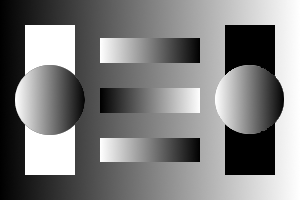
In this section we discuss the application of the TV-TV2 approach (5.2) to image denoising, where the operator equals the identity. We have performed experiments to images that have been corrupted with Gaussian noise, thus the norm in the fidelity term is the most suitable. We compare our method with infimal convolution [22] solved also with a split Bregman scheme and the total generalised variation [14] solved with the primal-dual method of Chambolle and Pock [23] as it is described in [13]. We present examples of (5.2) for , and , . Note that for , our model corresponds to the classical Rudin-Osher-Fatemi (ROF) denoising model, while for it corresponds to the pure TV2 restoration [8]. Our basic synthetic test image is shown in Figure 3.
Our main assessment for the quality of the reconstruction is the structural similarity index SSIM [73, 74]. The reason for that choice is that in contrast to traditional quality measures like the peak signal-to-noise ratio PSNR, the SSIM index also assesses the conservation of the structural information of the reconstructed image. Note that a perfect reconstruction has SSIM value equal to 1. A justification for the choice of SSIM as a good fidelity measure instead of the traditional PSNR can be seen in Figure 4. The second and the third image are denoising results with the first order method (, Gaussian noise, Variance = 0.5). The middle picture is the one with the highest SSIM value (0.6595) while the SSIM value of the right picture is significantly lower (0.4955). This assessment comes into an agreement with the human point of view since, even though this is subjective, one would consider the middle picture as a better reconstruction. On the other hand the middle picture has slightly smaller PSNR value (14.02) than the right one (14.63), which was the highest PSNR value. Similar results are obtained for .

As a stopping criterium for our algorithm we use a predefined number of iterations. In most examples this number is 300. We observe that after 80-100 iterations the relative residual of the iterates is of the order of or lower (see also Table 1) and hence no noticeable change in the iterates is observed after that.
In the following we shall examine whether the introduction of the higher-order term () in the denoising procedure, produces results of higher quality.

0.9053
0.8979
SSIM=0.9053
, SSIM=0.9081
, SSIM=0.8989
Post-processing: GIMP sharpening & contrast
The noise has been produced with MATLAB’s built in function imnoise.


SSIM=0.8168

, SSIM=0.8319

, SSIM=0.8185

SSIM=0.8171


SSIM=0.4436

, SSIM=0.8168

, ,
SSIM=0.8319

, ,
SSIM=0.8185

, SSIM=0.8171
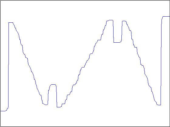
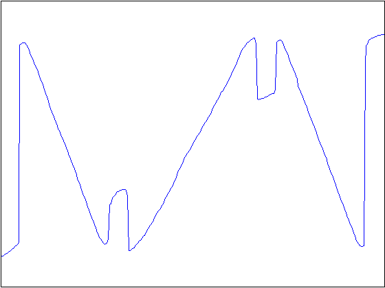
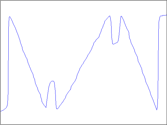
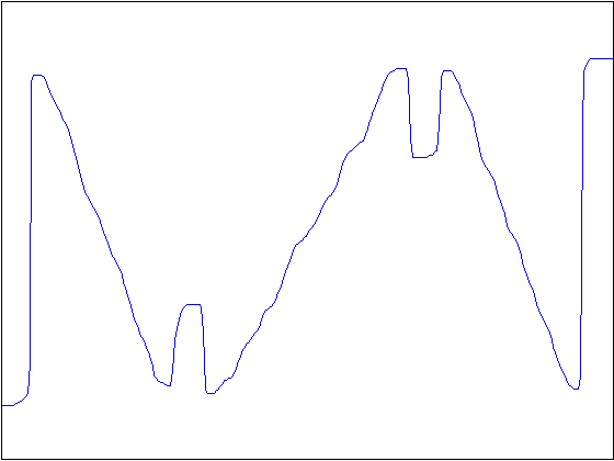
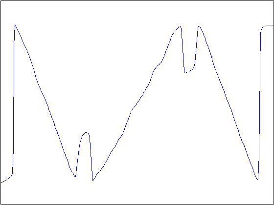
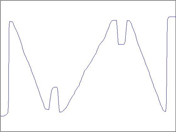
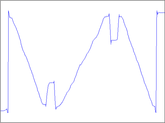
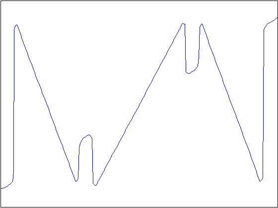
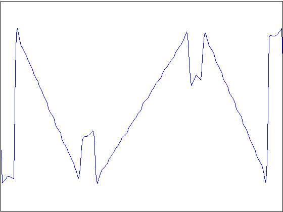
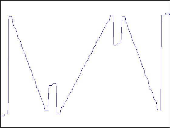
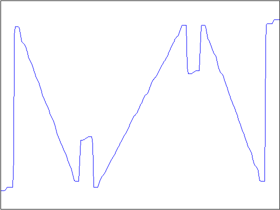
Figure 5 depicts one denoising example, where the original image is corrupted with Gaussian noise of variance 0.005. For better visualisation, we include the middle row slices of all the reconstructions in Figure 6. The highest SSIM value for TV denoising is achieved for (SSIM=0.8979) while the highest one for TV-TV2 is achieved for , (SSIM=0.9081). This is slightly better than infimal convolution (SSIM=0.9053). Note, however, that this optimal combination of and in terms of SSIM does not always correspond to best visual result. In general, the latter corresponds to a slightly bigger than the one chosen by SSIM, see Figure 5(h). Still, for proof of concept, we prefer to stick with an objective quality measure and SSIM, in our opinion, is the most reliable choice for that matter. In the image of Figure 5(h) the staircasing effect has almost disappeared and the image is still pleasant to the human eye despite being slightly more blurry. This slight blur, which is the price that the method pays for the removal of the staircasing effect, can be easily and efficiently removed in post-processing using simple sharpening filters, e.g. in GIMP. We did that in Figure 5(i), also adjusting the contrast, achieving a very good result both visually and SSIM-wise (0.9463).
The highest SSIM value is achieved by TGV (0.9249), delivering a reconstruction of very good quality. However, TGV converges slowly to the true solution. In order to check that, we compute the ground truth solution (denoted by ) for the parameters of the TGV problem that correspond to Figure 5(d), by taking a large amount of iterations (2000). We check the GPU time that is needed for the iterates to have a relative residual
and we do the same for the TV-TV2 example of Figure 5(f). For TGV, it takes 1297 iterations (primal-dual method [23]) and 36.25 seconds while for TV-TV2 it takes 86 split Bregman iterations and 4.05 seconds, see Table 1. That makes our method more suitable for cases where fast but not necessarily optimal results are needed, e.g. video processing.
In order to examine the quality of the reconstructions that are produced from each method as the number of iteration increases we have plotted in Figure 7 the evolution of SSIM values. In the horizontal axis, instead of the number of iterations we put the absolute CPU time calculated by the product of the number of iterations times the CPU time per iteration as it is seen in Table 1. We observe that, for TGV, the SSIM value increases gradually with time, while for the methods solved with split Bregman the image quality peaks very quickly and then remains almost constant except for TV where the staircasing appears in the later iterations.
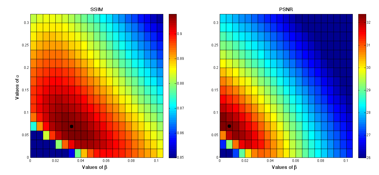
Next we check how the SSIM and PSNR values of the restored images behave as a function of the weighting parameters and . In Figure 8 we plot the results for and . The plots suggest that both quality measures behave in a continuous way and that they have a global maximum. However, PSNR tends to rate higher those images that have been processed with a small value of or even with which is not the case for SSIM. An explanation for that is that higher values of result to a further loss of contrast, see Figure 9, something that is penalised by the PSNR. The SSIM index penalises the loss of contrast as well but it also penalises the creation of the staircasing effect. This is another indication for the suitability of SSIM over PNSR. Note also, that the contrast can be recovered easily in a post-processing stage while it is not an easy task to reduce the staircasing effect using conventional processing tools.
Finally, in Figure 10 we perform denoising in an natural image which has been corrupted with Gaussian noise also of variance . The staircasing of TV denoising (SSIM=0.8168) is obvious in Figures 10(c) and (i). The overall best performance of the TV-TV2 method (SSIM=0.8319) is achieved by choosing , Figure 10(d). However, one can get satisfactory results by choosing (SSIM=0.8185), eliminating further the staircasing without blurring the image too much, compare for example the details in the Figures 10(j) and (k).
7. Applications in deblurring

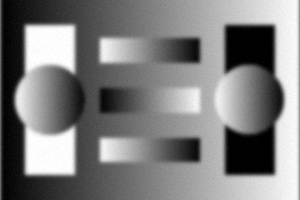
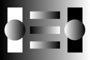
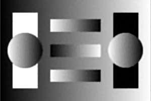
0.8003
0.9680

0.9466

0.9199

SSIM=0.8003
0.9680
SSIM=0.9466
SSIM=0.9199


SSIM=0.7149

SSIM=0.8293

, SSIM=0.8361

, SSIM=0.8307

, SSIM=0.8330,
Post-processing: GIMP sharpening


,SSIM=0.8293

, ,
SSIM=0.8361

, ,
SSIM=0.8307

Post-processing: GIMP
sharpening
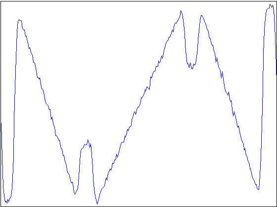
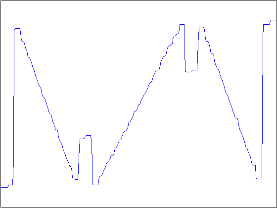
In our deblurring implementation denotes a circular convolution with a discrete approximation of a Gaussian kernel (, size: pixels). The blurred image is also corrupted by additive Gaussian noise of variance . Let us note here that the optimality condition (5.24) can be solved very fast using fast Fourier transforms. Deblurring results are shown in Figure 11 and the corresponding middle row slices in Figure 12. As in the denoising case the introduction of the second order term with a small weight decreases noticeably the staircasing effect, compare Figures (11)(c) and (f). Moreover, we can achieve better visual results if we increase further the value of without blurring the image significantly, Figure (11)(g). Infimal convolution does not give a satisfactory result here, Figure 11(e). TGV gives again the best qualitative result, Figure (11)(d), but the computation takes about 10 minutes. Even though the time comparison is not completely fair here (the implementation described in [13] does not use FFT) it takes a few thousands iterations for TGV to deblur the image satisfactorily, in comparison with a few hundreds for our TV-TV2 method.
In Figure 13 we discuss the performance of the TV-TV2 method for deblurring a natural image. The best result for the TV-TV2 method (SSIM=0.8361) is achieved with and , Figure 13(d). As in the case of denoising, one can increase the value of slightly, eliminating further the staircasing effect, Figures 13(e) and (k). The additional blur which is a result of the larger can be controlled using a sharpening filter, Figures 13(f) and (l).
8. Applications in inpainting




Finally, we present examples for the application of our TV-TV2 approach to image inpainting. There, the goal is to reconstruct an image inside a missing part using information from the intact part. The missing part is a domain , known as the inpainting domain. In this case the operator applied to an image gives
where as before is the characteristic function of , the intact part of the image domain. Let us note here that in cases of a small number of inpainting domains and a completely noise free and trustable image outside of the missing part, it is preferable to solve the inpainting problem only inside the holes, see for example [21]. However, here we would like to keep the method flexible, such that it includes the case where there is noise in the known regions as well.
In order to take advantage of the FFT for the optimality condition (5.24) a different splitting technique to (5.14) is required:
| (8.1) |
such that , , . We refer the reader to [57] for the details.
In Figure 14 we compare our method with harmonic and Euler’s elastica inpainting, see [25, 67]. In the case of harmonic inpainting the regulariser is the square of the norm of the gradient . In the case of Euler’s elastica the regulariser is
| (8.2) |
The minimisation of the Euler’s elastica energy corresponds to the minimisation of the length and curvature of the level lines of the image. Thus, this method is able to connect large gaps in the inpainting domain, see Figure 14(d). However, the term (8.2) is non-convex and thus difficult to be minimised. In order to implement Euler’s elastica inpainting we used the augmented Lagrangian method, proposed in [67]. There, the leading computational cost per iteration is due to the solution of one linear PDE and a system of linear PDEs (solved with FFT as well), in comparison to our approach which consists of one linear PDE only. Hence, in Table 1, we do not give absolute computational times as that would not be fair even more so because we did not optimise the Euler’s elastica algorithm with respect to the involved parameters. Moreover, it should be emphasised that the solution of TV-TV2 inpainting amounts to solve a convex problem while Euler’s elastica inpainting is a non-convex model.
In Figure 14 we see that, in contrast to harmonic and TV inpainting, TV2 inpainting is able to connect big gaps with the price of a blur, which can be controlled using a shock filter [2], see Figure 14(g). Notice that one has to choose small or even 0, in order to make the TV2 term dominant, compare Figures 14(e) and (f).
We also observe that in the TV2 case, the ability to connect large gaps depends on the size and geometry of the inpainting domain, see Figure 15 and also see [57] for more examples. Deriving sufficient conditions on the size and geometry of the inpainting domain for this connectivity to happen is a matter of future research.
Finally, in Figure 16 we compare TV, TV2 and Euler’s elastica, for its application to removing text (of large font) from a natural image. TV inpainting, Figure 16(b) gives unsatisfactory results, by producing piecewise constant results inside the inpainting domain, while the TV2 and Euler’s elastica results are comparable and seem to be visually closer to the true solution than the TV inpainted image.
9. Comparison with other higher-order methods
In the case of denoising and deblurring we compared our method with TGV, which we consider a state of the art method in the field of higher-order image reconstruction in the variational context. Indeed, in both image reconstruction tasks, TGV gives better qualitative results, in terms of the SSIM index. However the computational time that was needed to obtain the TGV result solved with the primal-dual method is significantly more than the one that is needed to compute the TV-TV2 method using split Bregman, see Table 1. We also show that with simple and fast post-processing techniques we can obtain results comparable with TGV. For these reasons, we think that the TV-TV2 approach is in particular interesting for applications in which the speed of computation matters. Regarding the comparison with inf-convolution, our method is slightly faster and results in better reconstructions in deblurring while in denoising the results are comparable. As far as inpainting is concerned, we compared our method (essentially the pure TV2 approach) with the Euler’s elastica, a higher-order variational method which is capable of giving very good results, by connecting large gaps in the inpainting domain. However, the regulariser there is non convex, something that could make the minimisation process produce a local minimiser instead of a global one. In TV2 the regulariser – regarded as a convex simplification of the Euler’s elastica idea – it has the ability to connect large gaps and the slight blur that is produced can be reduced by using a shock filter see for example [2, 45] and Figure 14(g). Moreover as we pointed out in the previous sections, our approach is computationally less expensive compared to TGV for image denoising and deblurring and Euler elastica for image inpainting.
| Denoising (B&W) – Image size: 200300 | ||||
| No of iterations for GT | No of iterations for | CPU time (secs) | time per iteration (secs) | |
| TV | 2000 | 136 | 2.86 | 0.0210 |
| TV2 | 2000 | 107 | 3.62 | 0.0338 |
| TV-TV2 | 2000 | 86 | 4.05 | 0.0471 |
| Inf.-Conv. | 2000 | 58 | 3.33 | 0.0574 |
| TGV | 2000 | 1297 | 36.25 | 0.0279 |
| Deblurring (B&W) – Image size: 200300 | ||||
| No of iterations for GT | No of iterations for | CPU time (secs) | time per iteration (secs) | |
| TV | 1000 | 478 | 10.72 | 0.0257 |
| TV2 | 1000 | 108 | 3.64 | 0.0337 |
| TV-TV2 | 1000 | 517 | 25.47 | 0.0493 |
| Inf.-Conv. | 1000 | 108 | 7.47 | 0.0692 |
| TGV | CPU time more than 10 minutes – see relevant comment in Section 7 | 1.22 | ||
| Inpainting (Colour) – Image size: 375500 | ||||
| No of iterations for | CPU time (secs) | time per iteration (secs) | ||
| TV | 88 | 26.67 | 0.3031 | |
| TV2 | 103 | 46.34 | 0.4499 | |
| E.e. | CPU time more than 10 minutes – see relevant comment in Section 8 | |||
10. Conclusion
We formulate a second order variational problem in the space of functions of bounded Hessian in the context of convex functions of measures. We prove existence and uniqueness of minimisers using a relaxation technique as well as stability. We propose the use of the split Bregman method for the numerical solution of the analogue discretised problem. The application of the split Bregman method to our model is quite robust and is converging after a few iterations. We perform numerical experiments by denoising images that have been corrupted by Gaussian noise, deblurring images that have been convoluted with Gaussian kernels, as well as in image inpainting.
In the case of denoising and deblurring, the introduction of the second order term leads to a significant reduction of the staircasing effect resulting in piecewise smooth images rather than piecewise constant images when using the ROF model. The superiority of an approach that combines first and second order regularisation rather than first order regularisation only, is confirmed quantitatively by the SSIM index. In the case of inpainting the higher-order method is able to connect edges along large gaps, a task that TV-inpainting is incapable of solving.
In summary, our approach is a simple and convex higher-order extension of total variation regularisation that improves the latter by reducing the staircasing effect in image denoising and deblurring, and by more faithfully respecting the good continuation principle in image inpainting. It can compete with other higher-order methods of its kind by giving almost comparable qualitative results while computing them in a fraction of time.
As fas as future work is concerned, a (not necessarily rigorous) rule for selecting the parameters and would be useful. Investigating the links with inf-convolution and spatially dependent regularisation on our model is also of interest. Moreover, the relation between the continuum and the discretised model could be investigated through -convergence arguments, see [30] and [12]. Finally the characterisation of subgradients of this approach and the analysis of solutions of the corresponding PDE flows for different choices of functions f and g promises to give more insight into the qualitative properties of this regularisation procedure. The characterisation of subgradients will also give more insight to properties of exact solutions of the minimisation of (1.1) concerning the avoidance of the staircasing effect.
Acknowledgements
The authors acknowledge the financial support provided by the Cambridge Centre for Analysis (CCA), the Royal Society International Exchanges Award IE110314 for the project “High-order Compressed Sensing for Medical Imaging”, the EPSRC / Isaac Newton Trust Small Grant “Non-smooth geometric reconstruction for high resolution MRI imaging of fluid transport in bed reactors” and the EPSRC first grant Nr. EP/J009539/1 “Sparse & Higher-order Image Restoration”. Further, this publication is based on work supported by Award No. KUK-I1-007-43 , made by King Abdullah University of Science and Technology (KAUST). We thank Clarice Poon for providing us with the Euler’s elastica code. Finally, we would like to thank the referees for their very useful comments and suggestions that improved the presentation of the paper.
Appendix A Some useful theorems
Proposition A.1.
Suppose that is a continuous function, positively homogeneous of degree and let . Then for every positive measure Radon measure such that is absolulely continuous with respect to , we have
Moreover, if is a convex function, then is a convex function as well.
Proof.
Since , we have that . Using the fact that is positively homogeneous and the fact that is a positive function, we get
Assuming that is convex and using the first part of the proposition we get for , , :
∎
The following theorem which is a special case of a theorem that was proved in [20] and can be also found in [4] establishes the lower semicontinuity of convex functionals of measures with respect to the weak∗ convergence.
Theorem A.2 (Buttazzo-Freddi, 1991).
Let be an open subset of , , be -valued finite Radon measures and , be positive Radon measures in . Let be a convex function and suppose that and weakly∗ in . Consider the Lebesgue decompositions , , . Then
In particular, if for all then according to the definition (2.1) the above inequality can be written as follows:
The following theorem is a special case of Theorem in [33].
Theorem A.3 (Demengel-Temam, 1984).
Suppose that is open, with Lipschitz boundary and let be a convex function from to with at most linear growth at infinity. Then for every there exists a sequence such that
Lemma A.4 (Kronecker’s lemma).
Suppose that and are two sequences of real numbers such that
and with . Then
In particular, if is a decreasing positive real sequence such that , then
References
- [1] R. Acar and C. R. Vogel. Analysis of bounded variation penalty methods for ill-posed problems. In Inverse Problems, pages 1217–1229, 1994.
- [2] L. Alvarez and L. Mazorra. Signal and image restoration using shock filters and anisotropic diffusion. SIAM Journal on Numerical Analysis, pages 590–605, 1994.
- [3] M. Amar and V. Cicco. Relaxation of quasi-convex integrals of arbitrary order. Proceedings of the Royal Society of Edinburgh: Section A Mathematics, 124(05):927–946, 1994.
- [4] L. Ambrosio, N. Fusco, and D. Pallara. Functions of bounded variation and free discontinuity problems. Oxford University Press, USA, 2000.
- [5] M. Benning. Singular Regularization of Inverse Problems. 2011.
- [6] M. Benning, C. Brune, M. Burger, and J. Müller. Higher-order TV methods – Enhancement via Bregman iteration. Journal of Scientific Computing, 54(2-3):269–310, 2013.
- [7] M. Benning and M. Burger. Error estimates for general fidelities. Electronic Transactions on Numerical Analysis, 38(44-68):77, 2011.
- [8] M. Bergounioux and L. Piffet. A second-order model for image denoising. Set Valued Anal. Variational Anal, 18(3-4):277–306, 2010.
- [9] A. Bertozzi, S. Esedoglu, and A. Gillette. Analysis of a two-scale Cahn-Hilliard model for binary image inpainting. Multiscale Modeling and Simulation, 6(3):913–936, 2008.
- [10] A. L. Bertozzi and J. B. Greer. Low-curvature image simplifiers: Global regularity of smooth solutions and Laplacian limiting schemes. Communications on Pure and Applied Mathematics, 57(6):764–790, 2004.
- [11] S. Boyd, N. Parikh, E. Chu, B. Peleato, and J. Eckstein. Distributed optimization and statistical learning via the alternating direction method of multipliers. Foundations and Trends in Machine Learning, 3(1):1–122, 2011.
- [12] A. Braides. -convergence for beginners. Oxford lecture series in mathematics and its applications, 2002.
- [13] K. Bredies. Recovering piecewise smooth multichannel images by minimization of convex functionals with total generalized variation penalty. Preprint, 2012.
- [14] K. Bredies, K. Kunisch, and T. Pock. Total generalized variation. SIAM Journal on Imaging Sciences, 3:1–42, 2009.
- [15] K. Bredies and D. Lorenz. Mathematische Bildverarbeitung: Einführung in Grundlagen und moderne Theorie. Vieweg+Teubner Verlag, 2011.
- [16] K. Bredies and T. Valkonen. Inverse problems with second-order total generalized variation constraints. In Proceedings of SampTA 2011 - 9th International Conference on Sampling Theory and Applications, Singapore, 2011.
- [17] M. Burger, L. He, and C. Schönlieb. Cahn-Hilliard inpainting and a generalization for grayvalue images. SIAM J. Imaging Sci., 2(4):1129–1167, 2009.
- [18] M. Burger and S. Osher. Convergence rates of convex variational regularization. Inverse problems, 20:1411, 2004.
- [19] M. Burger, E. Resmerita, and L. He. Error estimation for Bregman iterations and inverse scale space methods in image restoration. Computing, 81(2):109–135, 2007.
- [20] G. Buttazzo and L. Freddi. Functionals defined on measures and applications to non equi-uniformly elliptic problems. Annali di Matematica Pura ed Applicata, 159(1):133–149, 1991.
- [21] J. Cai, R. Chan, and Z. Shen. A framelet-based image inpainting algorithm. Applied and Computational Harmonic Analysis, 24(2):131–149, 2008.
- [22] A. Chambolle and P. Lions. Image recovery via total variation minimization and related problems. Numerische Mathematik, 76:167–188, 1997.
- [23] A. Chambolle and T. Pock. A first-order primal-dual algorithm for convex problems with applications to imaging. Journal of Mathematical Imaging and Vision, 40(1):120–145, 2011.
- [24] T. Chan and S. Esedoglu. Aspects of total variation regularized function approximation. SIAM Journal on Applied Mathematics, pages 1817–1837, 2005.
- [25] T. Chan, S. Kang, and J. Shen. Euler’s elastica and curvature-based inpainting. SIAM Journal on Applied Mathematics, 63(2):564–592, 2002.
- [26] T. Chan, A. Marquina, and P. Mulet. High-order total variation-based image restoration. SIAM J. Sci. Comput., 22(2):503–516, 2001.
- [27] T. F. Chan, S. Esedoglu, and F. Park. Image decomposition combining staircase reduction and texture extraction. J. Visual Communication and Image Representation, 18(6):464–486, 2007.
- [28] P. Charbonnier, L. Blanc-F raud, G. Aubert, and M. Barlaud. Two deterministic half-quadratic regularization algorithms for computed imaging. In ICIP (2)’94, pages 168–172, 1994.
- [29] P. Combettes, V. Wajs, et al. Signal recovery by proximal forward-backward splitting. Multiscale Modeling and Simulation, 4(4):1168–1200, 2006.
- [30] G. Dal Maso. Introduction to -convergence. Birkhauser, 1993.
- [31] G. Dal Maso, I. Fonseca, G. Leoni, and M. Morini. A higher order model for image restoration: the one dimensional case. SIAM J. Math. Anal, 40(6):2351–2391, 2009.
- [32] F. Demengel. Fonctions à Hessien borné. Ann. Inst. Fourier, 34:155–190, 1985.
- [33] F. Demengel and R. Temam. Convex functions of a measure and applications. Indiana Univ. Math. J., 33:673–709, 1984.
- [34] S. Didas, J. Weickert, and B. Burgeth. Properties of higher order nonlinear diffusion filtering. J. Math. Imaging Vis., 35:208–226, 2009.
- [35] Y. Dong, M. Hintermüller, F. Knoll, and R. Stollberger. Total variation denoising with spatially dependent regularization. In ISMRM 18th Annual Scientific Meeting and Exhibition Proceedings, page 5088, 2010.
- [36] V. Duval, J. Aujol, and Y. Gousseau. The TV model: a geometric point of view. SIAM journal on multiscale modeling and simulation, 8(1):154–189, 2009.
- [37] J. Eckstein. Splitting methods for monotone operators with applications to parallel optimisation. PhD thesis, 1989.
- [38] I. Ekeland and R. Témam. Convex Analysis and Variational Problems. Classics in Applied Mathematics. Society for Industrial and Applied Mathematics, 1999.
- [39] E. Esser, X. Zhang, and T. Chan. A general framework for a class of first order primal-dual algorithms for TV minimization. UCLA CAM Report 09-67, 2009.
- [40] L. Evans. Partial Differential Equations, volume 19 of Graduate Studies in Mathematics, Second Edition. American Mathematical Society,, 2010.
- [41] X. Feng and A. Prohl. Analysis of total variation flow and its finite element approximations. ESAIM-Mathematical Modelling and Numerical Analysis, 37(3):533, 2003.
- [42] K. Frick, P. Marnitz, and A. Munk. Statistical multiresolution estimation in imaging: Fundamental concepts and algorithmic framework. Electronic Journal of Statistics, 6:231–268, 2012.
- [43] C. Frohn-Schauf, S. Henn, and K. Witsch. Nonlinear multigrid methods for total variation image denoising. Computing and Visualization in Science, 7(3):199–206, 2004.
- [44] D. Gabay. Chapter IX applications of the method of multipliers to variational inequalities. In M. Fortin and R. Glowinski, editors, Augmented Lagrangian Methods: Applications to the Numerical Solution of Boundary-Value Problems, volume 15 of Studies in Mathematics and Its Applications, pages 299 – 331. Elsevier, 1983.
- [45] G. Gilboa, N. Sochen, and Y. Zeevi. Image enhancement and denoising by complex diffusion processes. Pattern Analysis and Machine Intelligence, IEEE Transactions on, 26(8):1020–1036, 2004.
- [46] T. Goldstein and S. Osher. The split Bregman method for regularized problems. SIAM Journal on Imaging Sciences, 2:323, 2009.
- [47] P. J. Green. Bayesian reconstructions from emission tomography data using a modified EM algorithm. IEEE Trans. Med. Imag, pages 84–93, 1990.
- [48] W. Hinterberger and O. Scherzer. Variational methods on the space of functions of bounded Hessian for convexification and denoising. Computing, 76:109–133, 2006.
- [49] G. Kanizsa. La Grammaire du Voir. Diderot, 1996.
- [50] R. Lai, X. Tai, and T. Chan. A ridge and corner preserving model for surface restoration. UCLA CAM Report 11-55, 2011.
- [51] S. Lefkimmiatis, A. Bourquard, and M. Unser. Hessian-based norm regularization for image restoration with biomedical applications. Image Processing, IEEE Transactions on, (99):1–1, 2010.
- [52] M. Lysaker, A. Lundervold, and X. C. Tai. Noise removal using fourth-order partial differential equation with applications to medical magnetic resonance images in space and time. IEEE Transactions on Image Processing, 12(12):1579–1590, 2003.
- [53] M. Lysaker and X. C. Tai. Iterative image restoration combining total variation minimization and a second-order functional. International Journal of Computer Vision, 66(1):5–18, 2006.
- [54] M. Nikolova. Minimizers of cost-functions involving nonsmooth data-fidelity terms. application to the processing of outliers. SIAM Journal on Numerical Analysis, pages 965–994, 2003.
- [55] M. Nikolova. A variational approach to remove outliers and impulse noise. Journal of Mathematical Imaging and Vision, 20(1):99–120, 2004.
- [56] S. Osher, M. Burger, D. Goldfarb, J. Xu, and W. Yin. An iterative regularization method for total variation-based image restoration. Multiscale Model. Simul., 4:460–489, 2005.
- [57] K. Papafitsoros, B. Sengul, and C. Schönlieb. Combined first and second order total variation inpainting using split Bregman. To appear in IPOL, 2013.
- [58] T. Pock, D. Cremers, H. Bischof, and A. Chambolle. Global solutions of variational models with convex regularization. SIAM Journal on Imaging Sciences, 3(4):1122–1145, 2010.
- [59] C. Pöschl. Tikhonov regularization with general residual term. PhD thesis, Leopold-Franzens-Universität Innsbruck, Austria, 2008.
- [60] C. Pöschl and O. Scherzer. Characterization of minimisers of convex regularization functionals. Contemporary mathematics, 451:219–248, 2008.
- [61] L. Rudin, S. Osher, and E. Fatemi. Nonlinear total variation based noise removal algorithms. Physica D: Nonlinear Phenomena, 60(1-4):259–268, 1992.
- [62] O. Scherzer. Denoising with higher order derivatives of bounded variation and an application to parameter estimation. jour-CASC, 60(1):1–27, 1998.
- [63] C. Schönlieb, A. Bertozzi, M. Burger, and L. He. Image inpainting using a fourth-order total variation flow. Proc. Int. Conf. SampTA09, Marseilles, 2009.
- [64] S. Setzer. Split Bregman algorithm, Douglas-Rachford splitting and frame shrinkage. Scale Space and Variational Methods in Computer Vision, 5567:464–476, 2009.
- [65] S. Setzer and G. Steidl. Variational methods with higher order derivatives in image processing. Approximation XII, pages 360–386, 2008.
- [66] S. Setzer, G. Steidl, and T. Teuber. Infimal convolution regularizations with discrete -type functionals. Comm. Math. Sci, 9:797–872, 2011.
- [67] X. Tai, J. Hahn, and G. Chung. A fast algorithm for Euler s elastica model using augmented Lagrangian method. SIAM Journal on Imaging Sciences, 4(1):313–344, 2011.
- [68] A. Tikhonov. Solution of incorrectly formulated problems and the regularization method. In Soviet Math. Dokl., volume 5, page 1035, 1963.
- [69] P. Vassilevski and J. G. Wade. A comparison of multilevel methods for total variation regularization. Elec. Trans. Numer. Anal, pages 6–255, 1997.
- [70] L. Vese. A study in the BV space of a denoising-deblurring variational problem. Applied Mathematics and Optimization, 44(2):131–161, 2001.
- [71] C. Vogel. A multigrid method for total variation-based image denoising. Progress in Systems and Control Theory, 20:323–323, 1995.
- [72] Y. Wang, W. Yin, and Y. Zhang. A fast algorithm for image deblurring with total variation regularization. Image Rochester NY, pages 1–19, 2007.
- [73] Z. Wang and A. Bovik. Mean squared error: Love it or leave it? a new look at signal fidelity measures. Signal Processing Magazine, IEEE, 26(1):98–117, 2009.
- [74] Z. Wang, A. Bovik, H. Sheikh, and E. Simoncelli. Image quality assessment: From error visibility to structural similarity. Image Processing, IEEE Transactions on, 13(4):600–612, 2004.
- [75] E. T. Whittaker. On a new method of graduation. Proceedings of the Edinburgh Mathematical Society, 41:63–75, 1923.
- [76] C. Wu and X. Tai. Augmented Lagrangian method, dual methods, and split Bregman iteration for ROF, vectorial TV, and high order models. SIAM Journal on Imaging Sciences, 3(3):300–339, 2010.
- [77] W. Yin, S. Osher, D. Goldfarb, and J. Darbon. Bregman iterative algorithms for -minimisation with applications to compressed sensing. SIAM J. Imaging Science, 1:142–168, 2008.