A Stochastic Gradient Method with an Exponential Convergence Rate for Finite Training Sets
Abstract
We propose a new stochastic gradient method for optimizing the sum of a finite set of smooth functions, where the sum is strongly convex. While standard stochastic gradient methods converge at sublinear rates for this problem, the proposed method incorporates a memory of previous gradient values in order to achieve a linear convergence rate. In a machine learning context, numerical experiments indicate that the new algorithm can dramatically outperform standard algorithms, both in terms of optimizing the training error and reducing the test error quickly.
1 Introduction
A plethora of the problems arising in machine learning involve computing an approximate minimizer of the sum of a loss function over a large number of training examples, where there is a large amount of redundancy between examples. The most wildly successful class of algorithms for taking advantage of this type of problem structure are stochastic gradient (SG) methods Robbins and Monro (1951); Bottou and LeCun (2003). Although the theory behind SG methods allows them to be applied more generally, in the context of machine learning SG methods are typically used to solve the problem of optimizing a sample average over a finite training set, i.e.,
| (1) |
In this work, we focus on such finite training data problems where each is smooth and the average function is strongly-convex.
As an example, in the case of -regularized logistic regression we have , where and are the training examples associated with a binary classification problem and is a regularization parameter. More generally, any -regularized empirical risk minimization problem of the form
| (2) |
falls in the framework of (1) provided that the loss functions are convex and smooth. An extensive list of convex loss functions used in machine learning is given by Teo et al. (2007), and we can even include non-smooth loss functions (or regularizers) by using smooth approximations.
The standard full gradient (FG) method, which dates back to Cauchy (1847), uses iterations of the form
| (3) |
Using to denote the unique minimizer of , the FG method with a constant step size achieves a linear convergence rate:
for some which depends on the condition number of (Nesterov, 2004, Theorem 2.1.15). Linear convergence is also known as geometric or exponential convergence, because the cost is cut by a fixed fraction on each iteration. Despite the fast convergence rate of the FG method, it can be unappealing when is large because its iteration cost scales linearly in . SG methods, on the other hand, have an iteration cost which is independent of , making them suited for that setting. The basic SG method for optimizing (1) uses iterations of the form
| (4) |
where is a step-size and a training example is selected uniformly among the set . The randomly chosen gradient yields an unbiased estimate of the true gradient , and one can show under standard assumptions that, for a suitably chosen decreasing step-size sequence , the SG iterations achieve the sublinear convergence rate
where the expectation is taken with respect to the selection of the variables. Under certain assumptions this convergence rate is optimal for strongly-convex optimization in a model of computation where the algorithm only accesses the function through unbiased measurements of its objective and gradient (see Nemirovski and Yudin (1983); Nemirovski et al. (2009); Agarwal et al. (2012)). Thus, we cannot hope to obtain a better convergence rate if the algorithm only relies on unbiased gradient measurements. Nevertheless, by using the stronger assumption that the functions are sampled from a finite dataset, in this paper we show that we can achieve an exponential converengence rate while preserving the iteration cost of SG methods.
The primay contribution of this work is the analysis of a new algorithm that we call the stochastic average gradient (SAG) method, a randomized variant of the incremental aggregated gradient (IAG) method Blatt et al. (2007), which combines the low iteration cost of SG methods with a linear convergence rate as in FG methods. The SAG method uses iterations of the form
| (5) |
where at each iteration a random training example is selected and we set
That is, like the FG method, the step incorporates a gradient with respect to each training example. But, like the SG method, each iteration only computes the gradient with respect to a single training example and the cost of the iterations is independent of . Despite the low cost of the SAG iterations, in this paper we show that the SAG iterations have a linear convergence rate, like the FG method. That is, by having access to and by keeping a memory of the most recent gradient value computed for each training example , this iteration achieves a faster convergence rate than is possible for standard SG methods. Further, in terms of effective passes through the data, we also show that for certain problems the convergence rate of SAG is faster than is possible for standard FG methods.
In a machine learning context where is a training cost associated with a predictor parameterized by , we are often ultimately interested in the testing cost, the expected loss on unseen data points. Note that a linear convergence rate for the training cost does not translate into a similar rate for the testing cost, and an appealing propertly of SG methods is that they achieve the optimal rate for the testing cost as long as every datapoint is seen only once. However, as is common in machine learning, we assume that we are only given a finite training data set and thus that datapoints are revisited multiple times. In this context, the analysis of SG methods only applies to the training cost and, although our analysis also focuses on the training cost, in our experiments the SAG method typically reached the optimal testing cost faster than both FG and SG methods.
The next section reviews closely-related algorithms from the literature, including previous attempts to combine the appealing aspects of FG and SG methods. However, despite years of extensive research on SG methods, most of the applications focusing on finite datasets, we are not aware of any other SG method that achieves a linear convergence rate while preserving the iteration cost of standard SG methods. Section 3 states the (standard) assumptions underlying our analysis and gives the main technical results; we first give a slow linear convergence rate that applies for any problem, and then give a very fast linear convergence rate that applies when is sufficiently large. Section 4 discusses practical implementation issues, including how to reduce the storage cost from to when each only depends on a linear combination of . Section 5 presents a numerical comparison of an implementation based on SAG to SG and FG methods, indicating that the method may be very useful for problems where we can only afford to do a few passes through a data set.
2 Related Work
There is a large variety of approaches available to accelerate the convergence of SG methods, and a full review of this immense literature would be outside the scope of this work. Below, we comment on the relationships between the new method and several of the most closely-related ideas.
Momentum: SG methods that incorporate a momentum term use iterations of the form
see Tseng (1998). It is common to set all for some constant , and in this case we can rewrite the SG with momentum method as
We can re-write the SAG updates (5) in a similar form as
| (6) |
where the selection function is equal to if corresponds to the last iteration where and is set to otherwise. Thus, momentum uses a geometric weighting of previous gradients while the SAG iterations select and average the most recent evaluation of each previous gradient. While momentum can lead to improved practical performance, it still requires the use of a decreasing sequence of step sizes and is not known to lead to a faster convergence rate.
Gradient Averaging: Closely related to momentum is using the sample average of all previous gradients,
which is similar to the SAG iteration in the form (5) but where all previous gradients are used. This approach is used in the dual averaging method Nesterov (2009), and while this averaging procedure leads to convergence for a constant step size and can improve the constants in the convergence rate Xiao (2010), it does not improve on the rate.
Iterate Averaging: Rather than averaging the gradients, some authors use the basic SG iteration but take an average over values. With a suitable choice of step-sizes, this gives the same asymptotic efficiency as Newton-like second-order SG methods and also leads to increased robustness of the convergence rate to the exact sequence of step sizes Polyak and Juditsky (1992). Baher’s method (Kushner and Yin, 2003, §1.3.4) combines gradient averaging with online iterate averaging, and also displays appealing asymptotic properties. The epoch SG method uses averaging to obtain the rate even for non-smooth objectives Hazan and Kale (2011). However, the convergence rates of these averaging methods remain sublinear.
Stochastic versions of FG methods: Various options are available to accelerate the convergence of the FG method for smooth functions, such as the accelerated full gradient (AFG) method Nesterov (1983), as well as classical techniques based on quadratic approximations such as non-linear conjugate gradient, quasi-Newton, and Hessian-free Newton methods. Several authors have analyzed stochastic variants of these algorithms Schraudolph (1999); Sunehag et al. (2009); Ghadimi and Lan (2010); Martens (2010); Xiao (2010). Under certain conditions these variants are convergent with an rate Sunehag et al. (2009). Alternately, if we split the convergence rate into a deterministic and stochastic part, these methods can improve the dependency on the deterministic part Ghadimi and Lan (2010); Xiao (2010). However, as with all other methods we have discussed thus far in this section, we are not aware of any existing method of this flavor that improves on the rate.
Constant step size: If the SG iterations are used with a constant step size (rather than a decreasing sequence), then the convergence rate of the method can be split into two parts (Nedic and Bertsekas, 2000, Proposition 2.4), where the first part depends on and converges linearly to and the second part is independent of but does not converge to . Thus, with a constant step size the SG iterations have a linear convergence rate up to some tolerance, and in general after this point the iterations do not make further progress. Indeed, convergence of the basic SG method with a constant step size has only been shown under extremely strong assumptions about the relationship between the functions Solodov (1998). This contrasts with the method we present in this work which converges to the optimal solution using a constant step size and does so with a linear rate (without additional assumptions).
Accelerated methods: Accelerated SG methods, which despite their name are not related to the aforementioned AFG method, take advantage of the fast convergence rate of SG methods with a constant step size. In particular, accelerated SG methods use a constant step size by default, and only decrease the step size on iterations where the inner-product between successive gradient estimates is negative Kesten (1958); Delyon and Juditsky (1993). This leads to convergence of the method and allows it to potentially achieve periods of linear convergence where the step size stays constant. However, the overall convergence rate of the method remains sublinear.
Hybrid Methods: Some authors have proposed variants of the SG method for problems of the form (1) that seek to gradually transform the iterates into the FG method in order to achieve a linear convergence rate. Bertsekas proposes to go through the data cyclically with a specialized weighting that allows the method to achieve a linear convergence rate for strongly-convex quadratic functions Bertsekas (1997). However, the weighting is numerically unstable and the linear convergence rate treats full passes through the data as iterations. A related strategy is to group the functions into ‘batches’ of increasing size and perform SG iterations on the batches Friedlander and Schmidt (2012). In both cases, the iterations that achieve the linear rate have a cost that is not independent of , as opposed to SAG.
Incremental Aggregated Gradient: Finally, Blatt et al. presents the most closely-related algorithm, the IAG method Blatt et al. (2007). This method is identical to the SAG iteration (5), but uses a cyclic choice of rather than sampling the values. This distinction has several important consequences. In particular, Blatt et al. are only able to show that the convergence rate is linear for strongly-convex quadratic functions (without deriving an explicit rate), and their analysis treats full passes through the data as iterations. Using a non-trivial extension of their analysis and a proof technique involving bounding the gradients and iterates simultaneously by a Lyapunov potential function, in this work we give an explicit linear convergence rate for general strongly-convex functions using the SAG iterations that only examine a single training example. Further, as our analysis and experiments show, when the number of training examples is sufficiently large, the SAG iterations achieve a linear convergence rate under a much larger set of step sizes than the IAG method. This leads to more robustness to the selection of the step size and also, if suitably chosen, leads to a faster convergence rate and improved practical performance. We also emphasize that in our experiments IAG and the basic FG method perform similarly, while SAG performs much better, showing that the simple change (random selection vs. cycling) can dramatically improve optimization performance.
3 Convergence Analysis
In our analysis we assume that each function in (1) is differentiable and that each gradient is Lipschitz-continuous with constant , meaning that for all and in we have
This is a fairly weak assumption on the functions, and in cases where the are twice-differentiable it is equivalent to saying that the eigenvalues of the Hessians of each are bounded above by . In addition, we also assume that the average function is strongly-convex with constant , meaning that the function is convex. This is a stronger assumption and is not satisfied by all machine learning models. However, note that in machine learning we are typically free to choose the regularizer, and we can always add an -regularization term as in Eq. (2) to transform any convex problem into a strongly-convex problem (in this case we have ). Note that strong-convexity implies that the problem is solvable, meaning that there exists some unique that achieves the optimal function value. Our convergence results assume that we initialize to a zero vector for all , and our results depend on the variance of the gradient norms at the optimum , denoted by . Finally, all our convergence results consider expectations with respect to the internal randomization of the algorithm, and not with respect to the data (which are assumed to be deterministic and fixed).
We first consider the convergence rate of the method when using a constant step size of , which is similar to the step size needed for convergence of the IAG method in practice.
Proposition 1
With a constant step size of , the SAG iterations satisfy for :
The proof is given in the Appendix. Note that the SAG iterations also trivially obtain the rate achieved by SG methods, since
albeit with a constant which is proportional to . Despite this constant, they are advantageous over SG methods in later iterations because they obtain an exponential convergence rate as in FG methods. We also note that an exponential convergence rate is obtained for any constant step size smaller than .
In terms of passes through the data, the rate in Proposition 1 is similar to that achieved by the basic FG method. However, our next result shows that, if the number of training examples is slightly larger than (which will often be the case, as discussed in Section 6), then the SAG iterations can use a larger step size and obtain a better convergence rate that is independent of and (see proof in the Appendix).
Proposition 2
If , with a step size of the SAG iterations satisfy for :
We state this result for because we assume that the first iterations of the algorithm use an SG method and that we initialize the subsequent SAG iterations with the average of the iterates, which leads to an rate. In contrast, using the SAG iterations from the beginning gives the same rate but with a constant proportional to . Note that this bound is obtained when initializing all to zero after the SG phase.111While it may appear suboptimal to not use the gradients computed during the iterations of stochastic gradient descent, using them only improves the bound by a constant. However, in our experiments we do not use the SG initialization but rather use a minor variant of SAG (discussed in the next section), which appears more difficult to analyze but which gives better performance.
It is interesting to compare this convergence rate with the known convergence rates of first-order methods (Nesterov, 2004, see §2). For example, if we take , , and then the basic FG method has a rate of and the ‘optimal’ AFG method has a faster rate of . In contrast, running iterations of SAG has a much faster rate of using the same number of evaluations of . Further, the lower-bound for a black-box first-order method is , indicating that SAG can be substantially faster than any FG method that does not use the structure of the problem.222Note that in the SAG rates is based on the functions, while in the FG methods it is based on which can be much smaller. In the Appendix, we compare Propositions 1 and 2 to the rates of primal and dual FG and coordinate-wise methods for the special case of -regularized leasts squares.
Even though appears in the convergence rate, if we perform iterations of SAG (i.e., one effective pass through the data), the error is multiplied by , which is independent of . Thus, each pass through the data reduces the excess cost by a constant multiplicative factor that is independent of the problem, as long as . Further, while the step size in Proposition 2 depends on and , we can obtain the same convergence rate by using a step size as large as . This is because the proposition is true for all values of satisfying , so we can choose the smallest possible value of . We have observed in practice that the IAG method with a step size of may diverge, even under these assumptions. Thus, for certain problems the SAG iterations can tolerate a much larger step size, which leads to increased robustness to the selection of the step size. Further, as our analysis and experiments indicate, the ability to use a large step size leads to improved performance of the SAG iterations.
While we have stated Proposition 1 in terms of the iterates and Proposition 2 in terms of the function values, the rates obtained on iterates and function values are equivalent because, by the Lipschitz and strong-convexity assumptions, we have .
4 Implementation Details
In this section we describe modifications that substantially reduce the SAG iteration’s memory requirements, as well as modifications that lead to better practical performance.
Structured gradients: For many problems the storage cost of for the vectors is prohibitive, but we can often use structure in the to reduce this cost. For example, many loss functions take the form for a vector . Since is constant, for these problems we only need to store the scalar for rather than the full gradient , reducing the storage cost to . Further, because of the simple form of the SAG updates, if is sparse we can use ‘lazy updates’ in order to reduce the iteration cost from down to the sparsity level of .
Mini-batches: To employ vectorization and parallelism, practical SG implementations often group training examples into ‘mini-batches’ and perform SG iterations on the mini-batches. We can also use mini-batches within the SAG iterations, and for problems with dense gradients this decreases the storage requirements of the algorithm since we only need a for each mini-batch. Thus, for example, using mini-batches of size leads to a 100-fold reduction in the storage cost.
Step-size re-weighting: On early iterations of the SAG algorithm, when most are set to the uninformative zero vector, rather than dividing in (5) by we found it was more effective to divide by , the number of unique values that we have sampled so far (which converges to ). This modification appears more difficult to analyze, but with this modification we found that the SAG algorithm outperformed the SG/SAG hybrid algorithm analyzed in Proposition 2.
Exact regularization: For regularized objectives like (2) we can use the exact gradient of the regularizer, rather than approximating it. For example, our experiments on -regularized optimization problems used the recursion
| (7) |
This can be implemented efficiently for sparse data sets by using the representation , where is a scalar and is a vector, since the update based on the regularizer simply updates .
Large step sizes: Proposition 1 requires while under an additional assumption Proposition 2 allows . In practice we observed better performance using step sizes of and . These step sizes seem to work even when the additional assumption of Proposition 2 is not satisfied, and we conjecture that the convergence rates under these step sizes are much faster than the rate obtained in Proposition 1 for the general case.
Line search: Since is generally not known, we experimented with a basic line-search, where we start with an initial estimate , and we double this estimate whenever we do not satisfy the instantiated Lipschitz inequality
To avoid instability caused by comparing very small numbers, we only do this test when . To allow the algorithm to potentially achieve a faster rate due to a higher degree of local smoothness, we multiply by after each iteration.
5 Experimental Results
Our experiments compared an extensive variety of competitive FG and SG methods. Our first experiments focus on the following methods, which we chose because they have no dataset-dependent tuning parameters:
-
–
Steepest: The full gradient method described by iteration (3), with a line-search that uses cubic Hermite polynomial interpolation to find a step size satisfying the strong Wolfe conditions, and where the parameters of the line-search were tuned for the problems at hand.
- –
-
–
L-BFGS: A publicly-available limited-memory quasi-Newton method that has been tuned for log-linear models.333http://www.di.ens.fr/~mschmidt/Software/minFunc.html This method is by far the most complicated method we considered.
- –
-
–
RDA: The regularized dual averaging method Xiao (2010), another recent state-of-the-art SG method.
-
–
ESG: The epoch SG method Hazan and Kale (2011), which runs SG with a constant step size and averaging in a series of epochs, and is optimal for non-smooth stochastic strongly-convex optimization.
-
–
NOSG: The nearly-optimal SG method Ghadimi and Lan (2010), which combines ideas from SG and AFG methods to obtain a nearly-optimal dependency on a variety of problem-dependent constants.
-
–
SAG: The proposed stochastic average gradient method described by iteration (5) using the modifications discussed in the previous section. We used a step-size of where is either set constant to the global Lipschitz constant (SAG-C) or set by adaptively estimating the constant with respect to the logistic loss function using the line-search described in the previous section (SAG-LS). The SAG-LS method was initialized with .
The theoretical convergence rates suggest the following strategies for deciding on whether to use an FG or an SG method:
-
1.
If we can only afford one pass through the data, then an SG method should be used.
-
2.
If we can afford to do many passes through the data (say, several hundred), then an FG method should be used.
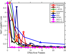
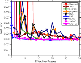
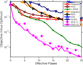
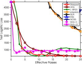
We expect that the SAG iterations will be most useful between these two extremes, where we can afford to do more than one pass through the data but cannot afford to do enough passes to warrant using FG algorithms like L-BFGS. To test whether this is indeed the case on real data sets, we performed experiments on a set of freely available benchmark binary classification data sets. The quantum (, ) and protein (, ) data set was obtained from the KDD Cup 2004 website,444http://osmot.cs.cornell.edu/kddcup the sido data set was obtained from the Causality Workbench website,555 http://www.causality.inf.ethz.ch/home.php while the rcv1 (, ) and covertype (, ) data sets were obtained from the LIBSVM data website.666 http://www.csie.ntu.edu.tw/~cjlin/libsvmtools/datasets Although our method can be applied to any differentiable function, on these data sets we focus on the -regularized logistic regression problem, with . We split each dataset in two, training on one half and testing on the other half. We added a (regularized) bias term to all data sets, and for dense features we standardized so that they would have a mean of zero and a variance of one. We measure the training and testing costs as a function of the number of effective passes through the data, measured as the number of evaluations divided by . These results are thus independent of the practical implementation of the algorithms. We plot the training and testing costs of the different methods for 30 effective passes through the data in Figure 1.
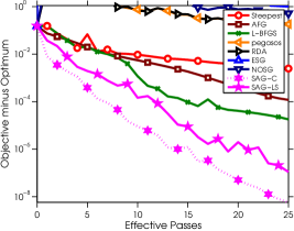
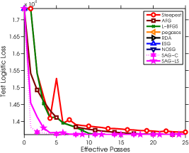
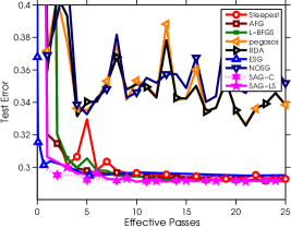
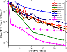
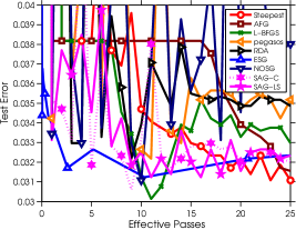
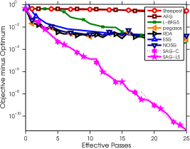
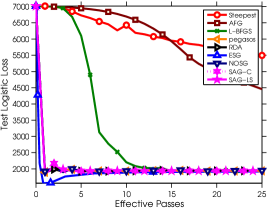
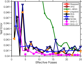
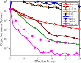
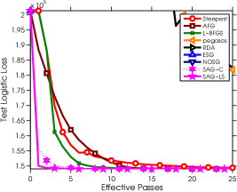
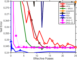
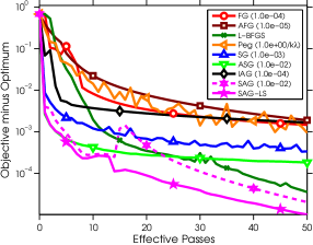
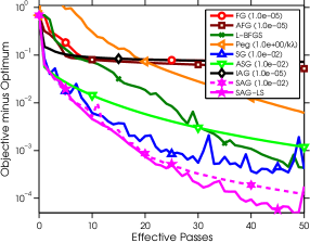
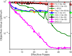
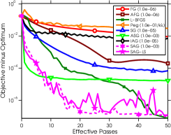
In our second series of experiments, we sought to test whether SG methods (or the IAG method) with a very carefully chosen step size would be competitive with the SAG iterations. In particular, we compared the following variety of basic FG and SG methods.
-
1.
FG: The full gradient method described by iteration (3).
- 2.
-
3.
peg: The pegasos algorithm of Shalev-Shwartz et al. (2007), but where we multiply the step size by a constant.
-
4.
SG: The stochastic gradient method described by iteration (4), where we use a constant step-size.
-
5.
ASG: The stochastic gradient method described by iteration (4), where we use a constant step size and average the iterates.777We have also compared to a variety of other SG methods, such as SG with momentum, SG with gradient averaging, accelerated SG, and using SG but delaying averaging until after the first effective pass. However, none of these SG methods performed better than the ASG method above so we omit them to keep the plots simple.
- 6.
-
7.
SAG: The proposed stochastic average gradient method described by iteration (5).
For all of the above methods, we chose the step size that gave the best performance among powers of . On the full data sets, we compare these methods to each other and to the L-BFGS and the SAG-LS algorithms from the previous experiment in Figure 2, which also shows the selected step sizes.
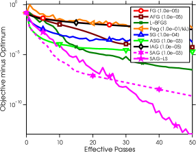
We can observe several trends across these experiments:
-
–
FG vs. SG: Although the performance of SG methods can be catastrophic if the step size is not chosen carefully (e.g., the quantum and covertype data), with a carefully-chosen step-size the SG methods always do substantially better than FG methods on the first few passes through the data. In contrast, the adaptive FG methods in the first experiment are not sensitive to the step size and because of its steady progress the best FG method (L-BFGS) always eventually passes the SG methods.
-
–
(FG and SG) vs. SAG: The SAG iterations seem to achieve the best of both worlds. They start out substantially better than FG methods, but continue to make steady (linear) progress which leads to better performance than SG methods. The significant speed-up observed for SAG in reaching low training costs often also seems to translate into reaching the optimal testing cost more quickly than the other methods. We also note that the proposed line-search seems to perform as well or better than choosing the optimal fixed step-size in hind sight.
-
–
IAG vs. SAG: The second experiment shows that the IAG method performs similarly to the regular FG method, and they also show the surprising result that the randomized SAG method outperforms the closely-related deterministic IAG method by a very large margin. This is due to the larger step sizes used by the SAG iterations, which would cause the IAG iterations to diverge.
6 Discussion
Optimal regularization strength: One might wonder if the additional hypothesis in Proposition 2 is satisfied in practice. In a learning context, where each function is the loss associated to a single data point, is equal to the largest value of the loss second derivative (1 for the square loss, 1/4 for the logistic loss) times , where is a the uniform bound on the norm of each data point. Thus, the constraint is satisfied when . In low-dimensional settings, the optimal regularization parameter is of the form Liang et al. (2009) where is a scalar constant, and may thus violate the constraint. However, the improvement with respect to regularization parameters of the form is known to be asymptotically negligible, and in any case in such low-dimensional settings, regular stochastic or batch gradient descent may be efficient enough in practice. In the more interesting high-dimensional settings where the dimension of our covariates is not small compared to the sample size , then all theoretical analyses we are aware of advocate settings of which satisfy this constraint. For example, Sridharan et al. (2008) considers parameters of the form in the parametric setting, while Eberts and Steinwart (2011) considers with in a non-parametric setting.
Training cost vs. testing cost: The theoretical contribution of this work is limited to the convergence rate of the training cost. Though there are several settings where this is the metric of interest (e.g., variational inference in graphical models), in many cases one will be interested in the convergence speed of the testing cost. Since the convergence rate of the testing cost, achieved by SG methods with decreasing step sizes (and a single pass through the data), is provably optimal when the algorithm only accesses the function through unbiased measurements of the objective and its gradient, it is unlikely that one can obtain a linear convergence rate for the testing cost with the SAG iterations. However, as shown in our experiments, the testing cost of the SAG iterates often reaches its minimum quicker than existing SG methods, and we could expect to improve the constant in the convergence rate, as is the case with online second-order methods Bottou and Bousquet (2007).
Step-size selection and termination criteria: The three major disadvantages of SG methods are: (i) the slow convergence rate, (ii) deciding when to terminate the algorithm, and (iii) choosing the step size while running the algorithm. This paper showed that the SAG iterations achieve a much faster convergence rate, but the SAG iterations may also be advantageous in terms of tuning step sizes and designing termination criteria. In particular, the SAG iterations suggest a natural termination criterion; since the average of the variables converges to as converges to zero, we can use as an approximation of the optimality of . Further, while SG methods require specifying a sequence of step sizes and mispecifying this sequence can have a disastrous effect on the convergence rate (Nemirovski et al., 2009, §2.1), our theory shows that the SAG iterations iterations achieve a linear convergence rate for any sufficiently small constant step size and our experiments indicate that a simple line-search gives strong performance.
Acknowledgements
Nicolas Le Roux, Mark Schmidt, and Francis Bach are supported by the European Research Council (SIERRA-ERC-239993). Mark Schmidt is also supported by a postdoctoral fellowship from the Natural Sciences and Engineering Research Council of Canada (NSERC).
Appendix
In this Appendix, we first give the proofs of the two propositions. Subsequently, we compare the convergence rates of primal and dual FG and coordinate-wise methods to the rates of SAG for -regularized least squares in terms of effective passes through the data.
Appendix A Proofs of the propositions
A.1 Problem set-up and notations
We use to denote a strongly convex function, where the functions , are convex functions from to with -Lipschitz continuous gradients. Let us denote by the unique minimizer of .
For , the stochastic average gradient algorithm performs the recursion
where an is selected in uniformly at random and we set
Denoting a random variable which takes the value with probability and otherwise (thus with zero expectation), this is equivalent to
with
Using this definition of , we have . Note that, for a given , the variables are not independent.
We also use the notation
Finally, if is a matrix and is a matrix, then:
-
•
is the matrix being the concatenation of the ()-blocks on the diagonal of ;
-
•
is the block-diagonal matrix whose ()-blocks on the diagonal are equal to the ()-blocks of .
A.2 Outline of the proofs
Each Proposition will be proved in multiple steps.
-
1.
We shall find a Lyapunov function from to such that the sequence decreases at a linear rate.
- 2.
-
3.
In the case of Proposition 2, we show how using one pass of stochastic gradient as the initialization provides the desired result.
Throughout the proofs, will denote the -field of information up to (and including time ), i.e., is the -field generated by .
A.3 Convergence results for stochastic gradient descent
The constant in both our bounds depends on the initialization chosen. While this does not affect the linear convergence of the algorithm, the bound we obtain for the first few passes through the data is the rate one would get using stochastic gradient descent, but with a constant proportional to . This problem can be alleviated for the second bound by running stochastic gradient descent for a few iterations before running the SAG algorithm. In this section, we provide bounds for the stochastic gradient descent algorithm which will prove useful for the SAG algorithm.
The assumptions made in this section about the functions and the function are the same as the ones used for SAG. To get initial values for and , we will do one pass of standard stochastic gradient.
We denote by the variance of the gradients at the optimum. We will use the following recursion:
Denoting , we have (following Bach and Moulines (2011))
Indeed, we have
By taking expectations, we get
Thus, if we take
we have and
Averaging from to and using the convexity of , we have
A.4 Important lemma
In both proofs, our Lyapunov function contains a quadratic term for some values of , and . The lemma below computes the value of in terms of elements of .
Lemma 1
If , for , and , then
with
Note that for square matrix, denotes a vector of size composed of the diagonal of , while for a vector of dimension , is the diagonal matrix with on its diagonal. Thus is a diagonal matrix with the diagonal elements of on its diagonal, and .
Proof Throughout the proof, we will use the equality . Moreover, all conditional expectations of linear functions of will be equal to zero.
We have
| (10) | |||
| (11) |
The first term (within the expectation) on the right-hand side of Eq. (11) is equal to
The only random term (given ) is the third one whose expectation is equal to
The second term (within the expectation) on the right-hand side of Eq. (11) is equal to
The only random term (given ) is the last one whose expectation is equal to
The last term on the right-hand side of Eq. (11) is equal to
The only random term (given ) is the last one whose expectation is equal to
Summing all these terms together, we get the following result:
with .
Rewriting , we have
Hence, the sum may be rewritten as
This concludes the proof.
A.5 Analysis for
We now prove Proposition 1, providing a bound for the convergence rate of the SAG algorithm in the case of a small step size, .
Proof
Step 1 - Linear convergence of the Lyapunov function
In this case, our Lyapunov function is quadratic, i.e.,
We consider
The goal will be to prove that is negative for some . This will be achieved by bounding all the terms by a term depending on whose positivity is guaranteed by the convexity of .
We have, with our definition of , and :
This leads to (using the lemma of the previous section):
The third line is obtained using the Lipschitz property of the gradient, that is
where the inequality in the second line stems from (Nesterov, 2004, Theorem 2.1.5).
We have
The difference is then:
Note that for any symmetric negative definite matrix and for any vectors and we have
and thus that
Using this fact with
we have
A sufficient condition for to be negative definite is to have .
The bound then becomes
We now use the strong convexity of to get the inequality
This yields the final bound
Since we know that is positive, due to the convexity of , we need to prove that is positive.
Using and gives
Hence,
We can then take a full expectation on both sides to obtain:
Since is a non-negative function (we show below that it dominates a non-negative function), this results proves the linear convergence of the sequence with rate . We have
Step 2 - Domination of by
We now need to prove that dominates . If is positive definite, then .
We shall use the Schur complement condition for positive definiteness. Since is positive definite, the other condition to verify is .
and so dominates .
This yields
We have
Initializing all the to 0, we get
and
A.6 Analysis for
Step 1 - Linear convergence of the Lyapunov function
We now prove Proposition 2, providing a bound for the convergence rate of the SAG algorithm in the case of a small step size, .
We shall use the following Lyapunov function:
with
This yields
We have
Our goal will now be to express all the quantities in terms of whose positivity is guaranteed by the convexity of .
Using the convexity of , we have
Using the Lipschitz property of the gradients of , we have
Using , we have
Reassembling all the terms together, we get
Using the convexity of gives
and, consequently,
If we regroup all the terms in together, and all the terms in together, we get
Let us rewrite this as
with
Assuming that and are negative, we have by completing the square that
where we used the fact that . After reorganization of the terms, we obtain
We now use the strong convexity of the function to get the following inequalities:
Finally, we have
If we choose with , , and , we get
Thus,
This quantity is negative for and . If we choose , then it is sufficient to have .
To finish the proof, we need to prove the positivity of the factor of .
Then, following the same argument as in the previous section, we have
with the variance of the gradients at the optimum.
Step 2 - Domination of by
We now need to prove that dominates .
| by dropping some terms. |
The quantity on the right-hand side is minimized for . Hence, we have
We thus get
Step 3 - Initialization of using stochastic gradient descent
During the first few iterations, we obtain the rate obtained using stochastic gradient descent, but with a constant which is proportional to . To circumvent this problem, we will first do iterations of stochastic gradient descent to initialize , which will be renamed to truly reflect the number of iterations done.
Appendix B Comparison of convergence rates
We consider the -regularized least squares problem
where to apply SG methods and SAG we can use
If we use to denote a vector containing the values and to denote a matrix withs rows , we can re-write this problem as
The Fenchel dual of this problem is
We can obtain the primal variables from the dual variables by the formula . Convergence rates of different primal and dual algorithms are often expressed in terms of the following Lipschitz constants:
| (Lipschitz constant of ) | |||
| (Lipschitz constant for all ) | |||
| (Lipschitz constant of all ) | |||
| (Lipschitz constant of ) | |||
| (Lipschitz constant of all ) |
Here, we use to denote the maximum eigenvalue of , to denote the maximum squared row-norm , and to denote the maximum squared column-norm . We use to refer to element of of , and similarly for . The convergence rates will also depend on the primal and dual strong-convexity constants:
| (Strong-convexity constant of ) | |||
| (Strong-convexity constant of ) |
Here, is the minimum eigenvalue of , and is the minimum eigenvalue of .
B.1 Full Gradient Methods
Using a similar argument to (Nesterov, 2004, Theorem 2.1.15), if we use the basic FG method with a step size of , then converges to zero with rate
while a larger step-size of gives a faster rate of
where the speed improvement is determined by the size of .
If we use the basic FG method on the dual problem with a step size of , then converges to zero with rate
and with a step-size of the rate is
Thus, whether we can solve the primal or dual method faster depends on and . In the over-determined case where has independent columns, a primal method should be preferred. In the under-determined case where has independent rows, we can solve the dual more efficiently. However, we note that a convergence rate on the dual objective does not necessarily yield the same rate in the primal objective. If is invertible (so that ) or it has neither independent columns nor independent rows (so that ), then there is no difference between the primal and dual rates.
The AFG method achieves a faster rate. Applied to the primal with a step-size of it has a rate of (Nesterov, 2004, Theorem 2.2.2)
and applied to the dual with a step-size of it has a rate of
B.2 Coordinate-Descent Methods
The cost of applying one iteration of an FG method is . For this same cost we could apply iterations of a coordinate descent method to the primal, assuming that selecting the coordinate to update has a cost of . If we select coordinates uniformly at random, then the convergence rate for iterations of coordinate descent with a step-size of is (Nesterov, 2010, Theorem 2)
Here, we see that applying a coordinate-descent method can be much more efficient than an FG method if . This can happen, for example, when the number of variables is much larger than the number of examples . Further, it is possible for coordinate descent to be faster than the AFG method if the difference between and is sufficiently large.
For the cost of one iteration of the FG method, we could alternately perform iterations of coordinate descent on the dual problem. With a step size of this would obtain a rate on the dual objective of
which will be faster than the dual FG method if . This can happen, for example, when the number of examples is much larger than the number of variables . The difference between the primal and dual coordinate methods depends on compared to and compared to .
B.3 Stochastic Average Gradient
For the cost of one iteration of the FG method, we can perform iterations of SAG. With a step size of , performing iterations of the SAG algorithm has a rate of
This is most similar to the rate obtained with the dual coordinate descent method, but is likely to be slower because of the term scaling . However, the difference will be decreased for over-determined problems when .
Under the condition , with a step size of performing iterations of the SAG algorithm has a rate of
Note that depending on the constants this may or may not not be faster than coordinate descent methods. However, if we consider the typical case where with and , then if we have we obtain
Despite the constant of (which is likely to be highly sub-optimal), from these rates we see that SAG outperforms coordinate descent methods when is sufficiently large.
References
- Agarwal et al. [2012] A. Agarwal, P. L. Bartlett, P. Ravikumar, and M. J. Wainwright. Information-theoretic lower bounds on the oracle complexity of stochastic convex optimization. IEEE Transactions on Information Theory, 58(5), 2012.
- Bach and Moulines [2011] F. Bach and E. Moulines. Non-asymptotic analysis of stochastic approximation algorithms for machine learning. NIPS, 2011.
- Bertsekas [1997] D. P. Bertsekas. A new class of incremental gradient methods for least squares problems. SIAM Journal on Optimization, 7(4):913–926, 1997.
- Blatt et al. [2007] D. Blatt, A. O. Hero, and H. Gauchman. A convergent incremental gradient method with a constant step size. SIAM Journal on Optimization, 18(1):29–51, 2007.
- Bottou and Bousquet [2007] L. Bottou and O. Bousquet. The tradeoffs of large scale learning. NIPS, 2007.
- Bottou and LeCun [2003] L. Bottou and Y. LeCun. Large scale online learning. NIPS, 2003.
- Cauchy [1847] M. A. Cauchy. Méthode générale pour la résolution des systèmes d’équations simultanées. Comptes rendus des séances de l’Académie des sciences de Paris, 25:536–538, 1847.
- Delyon and Juditsky [1993] B. Delyon and A. Juditsky. Accelerated stochastic approximation. SIAM Journal on Optimization, 3(4):868–881, 1993.
- Eberts and Steinwart [2011] M. Eberts and I. Steinwart. Optimal learning rates for least squares SVMs using Gaussian kernels. NIPS, 2011.
- Friedlander and Schmidt [2012] M. P. Friedlander and M. Schmidt. Hybrid deterministic-stochastic methods for data fitting. SIAM Journal of Scientific Computing, 34(3):A1351–A1379, 2012.
- Ghadimi and Lan [2010] S. Ghadimi and G. Lan. Optimal stochastic‘ approximation algorithms for strongly convex stochastic composite optimization. Optimization Online, July, 2010.
- Hazan and Kale [2011] E. Hazan and S. Kale. Beyond the regret minimization barrier: an optimal algorithm for stochastic strongly-convex optimization. COLT, 2011.
- Kesten [1958] H. Kesten. Accelerated stochastic approximation. Annals of Mathematical Statistics, 29(1):41–59, 1958.
- Kushner and Yin [2003] H. J. Kushner and G. Yin. Stochastic approximation and recursive algorithms and applications. Springer-Verlag, Second edition, 2003.
- Liang et al. [2009] P. Liang, F. Bach, and M. I. Jordan. Asymptotically optimal regularization in smooth parametric models. NIPS, 2009.
- Liu et al. [2009] J. Liu, J. Chen, and J. Ye. Large-scale sparse logistic regression. KDD, 2009.
- Martens [2010] J. Martens. Deep learning via Hessian-free optimization. ICML, 2010.
- Nedic and Bertsekas [2000] A. Nedic and D. Bertsekas. Convergence rate of incremental subgradient algorithms. In Stochastic Optimization: Algorithms and Applications, pages 263–304. Kluwer Academic, 2000.
- Nemirovski and Yudin [1983] A. Nemirovski and D. B. Yudin. Problem complexity and method efficiency in optimization. Wiley, 1983.
- Nemirovski et al. [2009] A. Nemirovski, A. Juditsky, G. Lan, and A. Shapiro. Robust stochastic approximation approach to stochastic programming. SIAM Journal on Optimization, 19(4):1574–1609, 2009.
- Nesterov [1983] Y. Nesterov. A method for unconstrained convex minimization problem with the rate of convergence . Doklady AN SSSR, 269(3):543–547, 1983.
- Nesterov [2004] Y. Nesterov. Introductory lectures on convex optimization: A basic course. Springer, 2004.
- Nesterov [2009] Y. Nesterov. Primal-dual subgradient methods for convex problems. Mathematical programming, 120(1):221–259, 2009.
- Nesterov [2010] Y. Nesterov. Efficiency of coordinate descent methods on huge-scale optimization problems. CORE Discussion Paper, 2010.
- Polyak and Juditsky [1992] B. T. Polyak and A. B. Juditsky. Acceleration of stochastic approximation by averaging. SIAM Journal on Control and Optimization, 30(4):838–855, 1992.
- Robbins and Monro [1951] H. Robbins and S. Monro. A stochastic approximation method. Annals of Mathematical Statistics, 22(3):400–407, 1951.
- Schraudolph [1999] N. Schraudolph. Local gain adaptation in stochastic gradient descent. ICANN, 1999.
- Shalev-Shwartz et al. [2007] S. Shalev-Shwartz, Y. Singer, and N. Srebro. Pegasos: Primal estimated sub-gradient solver for svm. ICML, 2007.
- Solodov [1998] M. Solodov. Incremental gradient algorithms with stepsizes bounded away from zero. Computational Optimization and Applications, 11(1):23–35, 1998.
- Sridharan et al. [2008] K. Sridharan, S. Shalev-Shwartz, and N. Srebro. Fast rates for regularized objectives. NIPS, 2008.
- Sunehag et al. [2009] P. Sunehag, J. Trumpf, S. Vishwanathan, and N. Schraudolph. Variable metric stochastic approximation theory. International Conference on Artificial Intelligence and Statistics, 2009.
- Teo et al. [2007] C. H. Teo, Q. Le, A. J. Smola, and S. V. N. Vishwanathan. A scalable modular convex solver for regularized risk minimization. KDD, 2007.
- Tseng [1998] P. Tseng. An incremental gradient(-projection) method with momentum term and adaptive stepsize rule. SIAM Journal on Optimization, 8(2):506–531, 1998.
- Xiao [2010] L. Xiao. Dual averaging methods for regularized stochastic learning and online optimization. Journal of Machine Learning Research, 11:2543–2596, 2010.