Semiparametrically efficient inference based on signed ranks in symmetric independent component models

Abstract

We consider semiparametric location-scatter models for which the $p$-variate observation is obtained as $X=\Lambda Z+\mu$, where $\mu$ is a $p$-vector, $\Lambda$ is a full-rank $p\times p$ matrix and the (unobserved) random $p$-vector $Z$ has marginals that are centered and mutually independent but are otherwise unspecified. As in blind source separation and independent component analysis (ICA), the parameter of interest throughout the paper is $\Lambda$. On the basis of $n$ i.i.d. copies of $X$, we develop, under a symmetry assumption on $Z$, signed-rank one-sample testing and estimation procedures for $\Lambda$. We exploit the uniform local and asymptotic normality (ULAN) of the model to define signed-rank procedures that are semiparametrically efficient under correctly specified densities. Yet, as is usual in rank-based inference, the proposed procedures remain valid (correct asymptotic size under the null, for hypothesis testing, and root-$n$ consistency, for point estimation) under a very broad range of densities. We derive the asymptotic properties of the proposed procedures and investigate their finite-sample behavior through simulations.

and

t1Supported by the Academy of Finland. t2Supported by an A.R.C. contract of the Communauté Française de Belgique. Davy Paindaveine is also member of ECORE, the association between CORE and ECARES.

1 Introduction

In multivariate statistics, concepts of location and scatter are usually defined through affine transformations of a noise vector. To be more specific, assume that the observation $X$ is obtained through

$$X=\Lambda Z+\mu,$$ (1)

where $\mu$ is a $p$-vector, $\Lambda$ is a full-rank $p\times p$ matrix and $Z$ is some standardized random vector. The exact nature of the resulting location parameter $\mu$, mixing matrix parameter $\Lambda$, and scatter parameter $\Sigma=\Lambda\Lambda^{\prime}$ crucially depends on the standardization adopted.

The most classical assumption on $Z$ specifies that $Z$ is standard $p$-normal. Then $\mu$ and $\Sigma$ simply coincide with the mean vector $\mathrm{E}[X]$ and variance–covariance matrix $\operatorname{Var}[X]$ of $X$, respectively. In robust statistics, it is often rather assumed that $Z$ is spherically symmetric about the origin of $\mathbb{R}^{p}$—in the sense that the distribution of $OZ$ does not depend on the orthogonal $p\times p$ matrix $O$. The resulting model in (1) is then called the elliptical model. If $Z$ has finite second-order moments, then $\mu=\mathrm{E}[X]$ and $\Sigma=c\operatorname{Var}[X]$ for some $c>0$, but (1) allows to define $\mu$ and $\Sigma$ in the absence of any moment assumption.

This paper focuses on an alternative standardization of $Z$, for which $Z$ has mutually independent marginals with common median zero. The resulting model in (1)—the independent component (IC) model, say—is more flexible than the elliptical model, even if one restricts, as we will do, to vectors $Z$ with symmetrically distributed marginals. The IC model indeed allows for heterogeneous marginal distributions for $X$, whereas, in contrast, marginals in the elliptical model all share—up to location and scale—the same distribution, hence also the same tail weight. This severely affects the relevance of elliptical models for practical applications, particularly so for moderate to large dimensions, since it is then very unlikely that all variables share, for example, the same tail weight.

The IC model provides the most standard setup for independent component analysis (ICA), in which the mixing matrix $\Lambda$ is to be estimated on the basis of $n$ independent copies $X_{1},\ldots,X_{n}$ of $X$, the objective being to recover (up to a translation) the original unobservable independent signals $Z_{1},\ldots,Z_{n}$ by premultiplying the $X_{i}$’s with the resulting $\hat{\Lambda}^{-1}$. It is well known in ICA, however, that $\Lambda$ is severely unidentified: for any $p\times p$ permutation matrix $P$ and any full-rank diagonal matrix $D$, one can always write

$$X=[\Lambda PD][(PD)^{-1}Z]+\mu=\tilde{\Lambda}\tilde{Z}+\mu,$$ (2)

where $\tilde{Z}$ still has independent marginals with median zero. Provided that $Z$ has at most one Gaussian marginal, two matrices $\Lambda_{1}$ and $\Lambda_{2}$ may lead to the same distribution for $X$ in (1) if and only if they are equivalent (we will write $\Lambda_{1}\sim\Lambda_{2}$) in the sense that $\Lambda_{2}=\Lambda_{1}PD$ for some matrices $P$ and $D$ as in (2); see, for example, Th04 . In other words, under the assumption that $Z$ has at most one Gaussian marginal, permutations ($P$), sign changes and scale transformations ($D$) of the independent components are the only sources of unidentifiability for $\Lambda$.

This paper considers inference on the mixing matrix $\Lambda$. More precisely, because of the identifiability issues above, we rather consider a normalized version $L$ of $\Lambda$, where $L$ is a well-defined representative of the class of mixing matrices that are equivalent to $\Lambda$. This parameter $L$ is actually the parameter of interest in ICA: an estimate of $L$ will indeed allow one to recover the independent signals $Z_{1},\ldots,Z_{n}$ equally well as an estimate of any other $\Lambda$ with $\Lambda\sim L$. Interestingly, the situation is extremely similar when considering inference on $\Sigma$ in the elliptical model. There, $\Sigma$ is only identified up to a positive scalar factor, and it is often enough to focus on inference about the well-defined shape parameter $V=\Sigma/(\det\Sigma)^{1/p}$ (e.g., in PCA, principal directions, proportions of explained variance, etc. can be computed from $V$). Just as $L$ is a normalized version of $\Lambda$ in the IC model, $V$ is a normalized version of $\Sigma$ in the elliptical model, and in both classes of models, the normalized parameters actually are the natural parameters of interest in many inference problems. The similarities further extend to the semiparametric nature of both models: just as the density $g_{\|\cdot\|}$ of $\|Z\|$ in the elliptical model, the pdf $g_{r}$ of the various independent components $Z_{r}$, $r=1,\ldots,p$, in the IC model, can hardly be assumed to be known in practice.

These strong similarities motivate the approach we adopt in this paper: we plan to conduct inference on $L$ (hypothesis testing and point estimation) in the IC model by adopting the methodology that proved extremely successful in Ha06c , Ha06 for inference on $V$ in the elliptical model. This methodology combines semiparametrically efficient inference and invariance arguments. In the IC model, the fixed-$(\mu,\Lambda)$ nonparametric submodels (indexed by $g_{1},\ldots,g_{p}$) indeed enjoy a strong invariance structure that is parallel to the one of the corresponding elliptical submodels (indexed by $g_{\|\cdot\|}$). As in Ha06c , Ha06 , we exploit this invariance structure through a general result from HW03 that allows one to derive invariant versions of efficient central sequences, on the basis of which one can define semiparametrically efficient (at fixed target densities $g_{r}=f_{r}$, $r=1,\ldots,p$) invariant procedures. As the maximal invariant associated with the invariance structure considered turns out to be the vector of marginal signed ranks of the residuals, the proposed procedures are of a signed-rank nature and do not require to estimate densities. While they achieve semiparametric efficiency under correctly specified densities, they remain valid (correct asymptotic size under the null, for hypothesis testing, and root-$n$ consistency, for point estimation) under misspecified densities.

We will consider the problem of estimating $L$ and that of testing the null $\mathcal{H}_{0}\dvtx L=L_{0}$ against the alternative $\mathcal{H}_{1}\dvtx L\neq L_{0}$, for some fixed $L_{0}$. While point estimation is undoubtedly of primary importance for applications (e.g., in blind source separation), one might question the practical relevance of the testing problem considered, especially when $L_{0}$ is not the $p$-dimensional identity matrix. Solving this generic testing problem, however, is the main step in developing tests for any linear hypothesis on $L$, and we will explicitly describe the resulting tests in the sequel. An extensive study of these tests is beyond the scope of the present paper, though; we refer to IC for an extension of our tests to the particular case of testing the (linear) hypothesis that $L$ is block-diagonal, a problem that is obviously important in practice (nonrejection of the null would indeed allow practitioners to proceed with two separate, lower-dimensional, analyses). Testing linear hypotheses on $L$ includes many other testing problems of high practical relevance, such as testing that a given column of $L$ is equal to some fixed $p$-vector, and testing that a given entry of $L$ is zero—the practical importance of these two testing problems, in relation, for example, with functional magnetic resonance imaging (fMRI), is discussed in Ol11 .

The paper is organized as follows. In Section 2, we fix the notation and describe the model (Section 2.1), state the corresponding uniformly locally and asymptotically normal (ULAN) property that allows us to determine semiparametric efficiency bounds (Section 2.2) and then introduce, in relation with invariance arguments, rank-based efficient central sequences (Section 2.3). In Sections 3 and 4, we develop the resulting rank tests and estimators for the mixing matrix $L$, respectively. Our estimators actually require the delicate estimation of $2p(p-1)$ “cross-information coefficients,” an issue we solve in Section 4.2 by generalizing the method recently developed in r12 . In Section 5, simulations are conducted both to compare the proposed estimators with some competitors and to investigate the validity of asymptotic results—simulation results for hypothesis testing are provided in the supplementary article IP11a . Finally, the Appendix states some technical results (Appendix A) and reports proofs (Appendix B).

2 The model, the ULAN property and invariance arguments

2.1 The model

As we already explained, the IC model above suffers from severe identifiability issues for $\Lambda$. To solve this, we map each $\Lambda$ onto a unique representative $L=\Pi(\Lambda)$ of the collection of mixing matrices $\tilde{\Lambda}$ that satisfy $\tilde{\Lambda}\sim\Lambda$ (the equivalence class of $\Lambda$ for $\sim$). We propose the mapping

$$\Lambda\mapsto\Pi(\Lambda)=\Lambda D^{+}_{1}PD_{2},$$

where $D^{+}_{1}$ is the positive definite diagonal matrix that makes each column of $\Lambda D^{+}_{1}$ have Euclidean norm one, $P$ is the permutation matrix for which the matrix $B=(b_{ij})=\Lambda D^{+}_{1}P$ satisfies $|b_{ii}|>|b_{ij}|$ for all $i<j$ and $D_{2}$ is the diagonal matrix such that all diagonal entries of $\Pi(\Lambda)=\Lambda D^{+}_{1}PD_{2}$ are equal to one.

If one restricts to the collection $\mathcal{M}_{p}$ of mixing matrices $\Lambda$ for which no ties occur in the permutation step above, it can easily be shown that, for any $\Lambda_{1},\Lambda_{2}\in\mathcal{M}_{p}$, we have that $\Lambda_{1}\sim\Lambda_{2}$ iff $\Pi(\Lambda_{1})=\Pi(\Lambda_{2})$, so that this mechanism succeeds in identifying a unique representative in each class of equivalence (this is ensured with the double scaling scheme above, which may seem a bit complicated at first). Besides, $\Pi$ is then a continuously differentiable mapping from $\mathcal{M}_{p}$ onto $\mathcal{M}_{1p}:=\Pi(\mathcal{M}_{p})$. While ties may always be taken care of in some way (e.g., by basing the ordering on subsequent rows of the matrix $B$), they may prevent the mapping $\Pi$ to be continuous, which would cause severe problems and would prevent us from using the Delta method in the sequel. It is clear, however, that the restriction to $\mathcal{M}_{p}$ only gets rid of a few particular mixing matrices, and will not have any implications in practice.

The parametrization of the IC model we consider is then associated with

$$X=LZ+\mu,$$ (3)

where $\mu\in\mathbb{R}^{p}$, $L\in\mathcal{M}_{1p}$ and $Z$ has independent marginals with common median zero. Throughout, we further assume that $Z$ admits a density with respect to the Lebesgue measure on $\mathbb{R}^{p}$, and that it has $p$ symmetrically distributed marginals, among which at most one is Gaussian (as explained in the Introduction, this limitation on the number of Gaussian components is needed for $L$ to be identifiable). We will denote by $\mathcal{F}$ the resulting collection of densities for $Z$. Of course, any $g\in\mathcal{F}$ naturally factorizes into $g(z)=\prod_{r=1}^{p}g_{r}(z_{r})$, where $g_{r}$ is the symmetric density of $Z_{r}$.

The hypothesis under which $n$ mutually independent observations $X_{i}$, $i=1,\ldots,n$, are obtained from (3), where $Z$ has density $g\in\mathcal{F}$, will be denoted as $\mathrm{P}^{(n)}_{\vartheta,g}$, with $\vartheta=(\mu^{\prime},(\operatorname{vecd}^{\circ}L)^{\prime})^{\prime}\in\Theta=\mathbb{R}^{p}\times\operatorname{vecd}^{\circ}(\mathcal{M}_{1p})$, or alternatively, as $\mathrm{P}^{(n)}_{\mu,L,g}$; for any $p\times p$ matrix $A$, we write $\operatorname{vecd}^{\circ}A$ for the $p(p-1)$-vector obtained by removing the $p$ diagonal entries of $A$ from its usual vectorized form $\operatorname{vec}A$ (diagonal entries of $L$ are all equal to one, hence should not be included in the parameter).

The resulting semiparametric model is then

$$\mathcal{P}^{(n)}:=\bigcup_{g\in\mathcal{F}}\mathcal{P}_{g}^{(n)}:=\bigcup_{g\in\mathcal{F}}\bigcup_{\vartheta\in\Theta}\bigl{\{}\mathrm{P}^{(n)}_{\vartheta,g}\bigr{\}}.$$ (4)

Performing semiparametrically efficient inference on $\vartheta$, at a fixed $f\in\mathcal{F}$, typically requires that the corresponding parametric submodel $\mathcal{P}_{f}^{(n)}$ satisfies the uniformly locally and asymptotically normal (ULAN) property.

2.2 The ULAN property

As always, the ULAN property requires technical regularity conditions on $f$. In the present context, we need that each corresponding univariate pdf $f_{r}$, $r=1,\ldots,p$, is absolutely continuous (with derivative $f^{\prime}_{r}$, say) and satisfies

$$\sigma^{2}_{f_{r}}:=\int_{-\infty}^{\infty}y^{2}f_{r}(y)\,dy<\infty,\qquad\mathcal{I}_{f_{r}}:=\int_{-\infty}^{\infty}\varphi_{f_{r}}^{2}(y)f_{r}(y)\,dy<\infty$$

and

$$\mathcal{J}_{f_{r}}:=\int_{-\infty}^{\infty}y^{2}\varphi_{f_{r}}^{2}(y)f_{r}(y)\,dy<\infty,$$

where we let $\varphi_{f_{r}}:=-f^{\prime}_{r}/f_{r}$. In the sequel, we denote by $\mathcal{F}_{\mathrm{ulan}}$ the collection of pdfs $f\in\mathcal{F}$ meeting these conditions.

For any $f\in\mathcal{F}_{\mathrm{ulan}}$, let $\gamma_{rs}(f):=\mathcal{I}_{f_{r}}\sigma^{2}_{f_{s}}$, define the optimal $p$-variate location score function $\varphi_{f}\dvtx\mathbb{R}^{p}\to\mathbb{R}^{p}$ through $z=(z_{1},\ldots,z_{p})^{\prime}\mapsto\varphi_{f}(z)=(\varphi_{f_{1}}(z_{1}),\break\ldots,\varphi_{f_{p}}(z_{p}))^{\prime}$, and denote by $\mathcal{I}_{f}$ the diagonal matrix with diagonal entries $\mathcal{I}_{f_{r}}$, $r=1,\ldots,p$. Further write $I_{\ell}$ for the $\ell$-dimensional identity matrix and define

$$C:=\sum_{r=1}^{p}\sum_{s=1}^{p-1}\bigl{(}e_{r}e_{r}^{\prime}\otimes u_{s}e_{s+\delta_{[s\geq r]}}^{\prime}\bigr{)},$$

where $\otimes$ is the usual Kronecker product, $e_{r}$ and $u_{r}$ stand for the $r$th vectors of the canonical basis of $\mathbb{R}^{p}$ and $\mathbb{R}^{p-1}$, respectively, and $\delta_{[s\geq r]}$ is equal to one if $s\geq r$ and to zero otherwise. The following ULAN result then easily follows from Proposition 2.1 in IC by using a simple chain rule argument.

Proposition 2.1

Fix $f\in\mathcal{F}_{\mathrm{ulan}}$. Then the collection of probability distributions $\mathcal{P}_{f}^{(n)}$ is ULAN, with central sequence

$$\qquad\Delta_{\vartheta,f}=\pmatrix{\Delta_{\vartheta,f;1}\cr\Delta_{\vartheta,f;2}}=\pmatrix{\displaystyle n^{-1/2}(L^{-1})^{\prime}\sum_{i=1}^{n}\varphi_{f}(Z_{i})\vspace*{2pt}\cr\displaystyle n^{-1/2}C(I_{p}\otimes L^{-1})^{\prime}\sum_{i=1}^{n}\operatorname{vec}\bigl{(}\varphi_{f}(Z_{i})Z_{i}^{\prime}-I_{p}\bigr{)}},$$ (5)

where $Z_{i}=Z_{i}(\vartheta)=L^{-1}(X_{i}-\mu)$, and full-rank information matrix

$$\Gamma_{L,f}=\pmatrix{\Gamma_{L,f;1}&0\cr 0&\Gamma_{L,f;2}},$$

where $\Gamma_{L,f;1}:=(L^{-1})^{\prime}\mathcal{I}_{f}L^{-1}$ and

$$\Gamma_{L,f;2} := C(I_{p}\otimes L^{-1})^{\prime}\Biggl{[}\sum_{r=1}^{p}(\mathcal{J}_{f_{r}}-1)(e_{r}e_{r}^{\prime}\otimes e_{r}e_{r}^{\prime})$$

$$\hphantom{C(I_{p}\otimes L^{-1})^{\prime}\Biggl{[}}{}+\sum_{r,s=1,r\neq s}^{p}\bigl{(}\gamma_{sr}(f)(e_{r}e_{r}^{\prime}\otimes e_{s}e_{s}^{\prime})+(e_{r}e_{s}^{\prime}\otimes e_{s}e_{r}^{\prime})\bigr{)}\Biggr{]}$$

$${}\times(I_{p}\otimes L^{-1})C^{\prime}.$$

More precisely, for any $\vartheta_{n}=\vartheta+O(n^{-1/2})$ $($with $\vartheta=(\mu^{\prime},(\operatorname{vecd}^{\circ}L)^{\prime})^{\prime})$ and any bounded sequence $(\tau_{n})$ in $\mathbb{R}^{p^{2}}$, we have that, under $\mathrm{P}^{(n)}_{\vartheta_{n},f}$ as $n\rightarrow\infty$,

$$\log\bigl{(}d\mathrm{P}^{(n)}_{\vartheta_{n}+n^{-1/2}\tau_{n},f}/d\mathrm{P}^{(n)}_{\vartheta_{n},f}\bigr{)}=\tau_{n}^{\prime}\Delta_{\vartheta_{n},f}-\tfrac{1}{2}\tau_{n}^{\prime}\Gamma_{L,f}\tau_{n}+o_{\mathrm{P}}(1),$$

and $\Delta_{\vartheta_{n},f}$ converges in distribution to a $p^{2}$-variate normal distribution with mean zero and covariance matrix $\Gamma_{L,f}$.

Semiparametrically efficient (at $f$) inference procedures on $L$ then may be based on the so-called efficient central sequence $\Delta^{*}_{\vartheta,f;2}$ resulting from $\Delta_{\vartheta,f;2}$ by performing adequate tangent space projections; see Bi93 . Under $\mathrm{P}^{(n)}_{\vartheta,f}$, $\Delta^{*}_{\vartheta,f;2}$ is still asymptotically normal with mean zero, but now with covariance matrix $\Gamma^{*}_{L,f;2}$ (the efficient information matrix). This matrix $\Gamma^{*}_{L,f;2}$ settles the semiparametric efficiency bound at $f$ when performing inference on $L$. For instance, an estimator $\hat{L}$ is semiparametrically efficient at $f$ if

$$\sqrt{n}\operatorname{vecd}^{\circ}(\hat{L}-L)\stackrel{{\scriptstyle\mathcal{L}}}{{\to}}\mathcal{N}_{p(p-1)}(0,(\Gamma^{*}_{L,f;2})^{-1}).$$ (6)

The performance of semiparametrically efficient tests on $L$ can similarly be characterized in terms of $\Gamma^{*}_{L,f;2}$: a test of $\mathcal{H}_{0}\dvtx L=L_{0}$ is semiparametrically efficient at $f$ (at asymptotic level $\alpha$) if its asymptotic powers under local alternatives of the form $\mathcal{H}_{1}^{(n)}\dvtx L=L_{0}+n^{-1/2}H$, where $H$ is an arbitrary $p\times p$ matrix with zero diagonal entries, are given by

$$1-\Psi_{p(p-1)}\bigl{(}\chi^{2}_{p(p-1),1-\alpha};(\operatorname{vecd}^{\circ}H)^{\prime}\Gamma^{*}_{L_{0},f;2}(\operatorname{vecd}^{\circ}H)\bigr{)},$$ (7)

where $\chi^{2}_{p(p-1),1-\alpha}$ stands for the $\alpha$-upper quantile of the $\chi^{2}_{p(p-1)}$ distribution, and $\Psi_{p(p-1)}(\cdot;\delta)$ denotes the cumulative distribution function of the noncentral $\chi^{2}_{p(p-1)}$ distribution with noncentrality parameter $\delta$.

2.3 Invariance arguments

Instead of the classical tangent space projection approach to compute $\Delta^{*}_{\vartheta,f;2}$ (as in CB06 ), we adopt an approach—due to HW03 —that rather exploits the invariance structure of the model considered. This will provide a version of the efficient central sequence (parallel to central sequences, efficient central sequences are defined up to $o_{\mathrm{P}}(1)$’s only) that is based on signed ranks. Here, signed ranks are defined as $S_{i}(\vartheta)=(S_{i1}(\vartheta),\ldots,S_{ip}(\vartheta))^{\prime}$ and $R^{+}_{i}(\vartheta)=(R^{+}_{i1}(\vartheta),\ldots,R^{+}_{ip}(\vartheta))^{\prime}$, where $S_{ir}(\vartheta)$ is the sign of $Z_{ir}(\vartheta)=(L^{-1}(X_{i}-\mu))_{r}$ and $R^{+}_{ir}(\vartheta)$ is the rank of $|Z_{ir}(\vartheta)|$ among $|Z_{1r}(\vartheta)|,\ldots,|Z_{nr}(\vartheta)|$. This signed-rank efficient central sequence—$\underline{\Delta}^{*}_{\vartheta,f;2}$, say—is given in Theorem 2.1 below (the asymptotic behavior of $\underline{\Delta}^{*}_{\vartheta,f;2}$ will be studied in Appendix A).

To be able to state Theorem 2.1, we need to introduce the following notation. Let $z\mapsto F_{+}(z)=(F_{+1}(z_{1}),\ldots,F_{+r}(z_{p}))^{\prime}$, with $F_{+r}(t):=\mathrm{P}^{(n)}_{\vartheta,f}[|Z_{r}(\vartheta)|<t]=2(\int_{-\infty}^{t}f_{r}(s)\,ds)-1$, $t\geq 0$. Based on this, define $\underline{\Delta}^{*}_{\vartheta,f;2}:=C(I_{p}\otimes L^{-1})^{\prime}\*\operatorname{vec}\underline{T}_{\vartheta,f},$ with

$$\underline{T}_{\vartheta,f} := \operatorname{odiag}\Biggl{[}\frac{1}{\sqrt{n}}\sum_{i=1}^{n}\biggl{(}S_{i}(\vartheta)\odot\varphi_{f}\biggl{(}F_{+}^{-1}\biggl{(}\frac{R^{+}_{i}(\vartheta)}{n+1}\biggr{)}\biggr{)}\biggr{)}$$

$$\hphantom{\operatorname{odiag}\Biggl{[}\frac{1}{\sqrt{n}}\sum_{i=1}^{n}}\hskip 10.7pt{}\times\biggl{(}S_{i}(\vartheta)\odot F_{+}^{-1}\biggl{(}\frac{R^{+}_{i}(\vartheta)}{n+1}\biggr{)}\biggr{)}^{\prime}\Biggr{]},$$

where $\odot$ is the Hadamard (i.e., entrywise) product of two vectors, and where $\operatorname{odiag}(A)$ denotes the matrix obtained from $A$ by replacing all diagonal entries with zeros. Finally, let $\underline{\mathcal{F}}_{\mathrm{ulan}}$ be the collection of pdfs $f\in\mathcal{F}_{\mathrm{ulan}}$ for which each $\varphi_{f_{r}}$, $r=1,\ldots,p$, is continuous and can be written as the difference of two monotone increasing functions. We then have the following result (see Appendix B for a proof).

Theorem 2.1

Fix $\vartheta=(\mu^{\prime},(\operatorname{vecd}^{\circ}L)^{\prime})^{\prime}\in\Theta$ and $f\in\underline{\mathcal{F}}_{\mathrm{ulan}}$. Then, (i) denoting by $\mathrm{E}^{(n)}_{\vartheta,f}$ expectation under $\mathrm{P}^{(n)}_{\vartheta,f}$,

$$\underline{\Delta}^{*}_{\vartheta,f;2}:\! = C(I_{p}\otimes L^{-1})^{\prime}\operatorname{vec}\underline{T}_{\vartheta,f}$$

$$= \mathrm{E}^{(n)}_{\vartheta,f}[\Delta_{\vartheta,f;2}|S_{1}(\vartheta),\ldots,S_{n}(\vartheta),R^{+}_{1}(\vartheta),\ldots,R^{+}_{n}(\vartheta)]+o_{L^{2}}(1)$$

as $n\to\infty$, under $\mathrm{P}^{(n)}_{\vartheta,f}$; (ii) the signed-rank quantity $\underline{\Delta}^{*}_{\vartheta,f;2}$ is a version of the efficient central sequence at $f$ [i.e., $\underline{\Delta}^{*}_{\vartheta,f;2}=\Delta^{*}_{\vartheta,f;2}+o_{L^{2}}(1)$ as $n\to\infty$, under $\mathrm{P}^{(n)}_{\vartheta,f}$].

Would the (nonparametric) fixed-$\vartheta$ submodels $\mathcal{P}_{\vartheta}^{(n)}:=\bigcup_{g\in\mathcal{F}}\{\mathrm{P}^{(n)}_{\vartheta,g}\}$ of the semiparametric model $\bigcup_{\theta\in\Theta}\bigcup_{g\in\mathcal{F}}\{\mathrm{P}^{(n)}_{\theta,g}\}$ in (4) be invariant under a group of transformations $\mathcal{G}^{\vartheta}$ that generates $\mathcal{P}_{\vartheta}^{(n)}$, then the main result of HW03 would show that the expectation of the original central sequence $\Delta_{\vartheta,f;2}$ conditional upon the corresponding maximal invariant—$\mathcal{I}^{(n)}_{\max}(\vartheta)$, say—is a version of the efficient central sequence $\Delta^{*}_{\vartheta,f;2}$ at $f$: as $n\to\infty$, under $\mathrm{P}^{(n)}_{\vartheta,f}$,

$$\Delta^{*}_{\vartheta,f;2}=\mathrm{E}^{(n)}_{\vartheta,f}\bigl{[}\Delta_{\vartheta,f;2}|\mathcal{I}^{(n)}_{\max}(\vartheta)\bigr{]}+o_{L^{2}}(1).$$ (8)

Such an invariance structure actually exists and the relevant group $\mathcal{G}^{\vartheta}$ collects all transformations

$$g^{\vartheta}_{h}\dvtx\mathbb{R}^{p}\times\cdots\times\mathbb{R}^{p} \to \mathbb{R}^{p}\times\cdots\times\mathbb{R}^{p},$$

$$(x_{1},\ldots,x_{n}) \mapsto \bigl{(}Lh(z_{1}(\vartheta))+\mu,\ldots,Lh(z_{n}(\vartheta))+\mu\bigr{)},$$

with $z_{i}(\vartheta):=L^{-1}(x_{i}-\mu)$ and $h((z_{1},\ldots,z_{p})^{\prime})=(h_{1}(z_{1}),\ldots,h_{p}(z_{p}))^{\prime}$, where each $h_{r}$, $r=1,\ldots,p$, is continuous, odd, monotone increasing and fixes $+\infty$. It is easy to check that $\mathcal{P}_{\vartheta}^{(n)}$ is invariant under (and is generated by) $\mathcal{G}^{\vartheta}$, and that the corresponding maximal invariant is the vector of signed ranks

$$\mathcal{I}^{(n)}_{\max}(\vartheta)=(S_{1}(\vartheta),\ldots,S_{n}(\vartheta),R^{+}_{1}(\vartheta),\ldots,R^{+}_{n}(\vartheta));$$ (9)

Theorem 2.1(ii) then follows from (8) and Theorem 2.1(i).

Inference procedures based on $\underline{\Delta}^{*}_{\vartheta,f;2}$, unlike those (from CB06 ) based on the efficient central sequence $\Delta^{*}_{\vartheta,f;2}$ obtained through tangent space projections, are measurable with respect to signed ranks, hence enjoy all nice properties usually associated with rank methods: robustness, ease of computation, validity without density estimation (and, for hypothesis testing, even distribution-freeness), etc.

3 Hypothesis testing

We now consider the problem of testing the null hypothesis $\mathcal{H}_{0}\dvtx L=L_{0}$ against the alternative $\mathcal{H}_{1}\dvtx L\neq L_{0}$, with unspecified underlying density $g$. Beyond their intrinsic interest, the resulting tests will play an important role in the construction of the $R$-estimators of Section 4 below, and they pave the way to testing linear hypotheses on $L$.

The objective here is to define a test that is semiparametrically efficient at some target density $f$, yet that remains valid—in the sense that it meets asymptotically the level constraint—under a very broad class of densities $g$. As we will show, this objective is achieved by the signed-rank test—$\underline{\phi}_{f}$, say—that rejects $\mathcal{H}_{0}$ at asymptotic level $\alpha\in(0,1)$ whenever

$$\underline{Q}_{f}:=(\underline{\Delta}^{*}_{\hat{\vartheta}_{0},f;2})^{\prime}(\Gamma^{*}_{L_{0},f;2})^{-1}\underline{\Delta}^{*}_{\hat{\vartheta}_{0},f;2}>\chi^{2}_{p(p-1),1-\alpha},$$ (10)

where $\Gamma^{*}_{L,f;2}$ was introduced on Page 2.1 (an explicit expression is given below) and where $\hat{\vartheta}_{0}=(\hat{\mu}^{\prime},(\operatorname{vecd}^{\circ}L_{0})^{\prime})^{\prime}$ is based on a sequence of estimators $\hat{\mu}$ that is locally asymptotically discrete (see Appendix A for a precise definition) and root-$n$ consistent under the null.

Possible choices for $\hat{\mu}$ include (discretized versions of) the sample mean $\bar{X}:=\frac{1}{n}\sum_{i=1}^{n}X_{i}$ or the transformation-retransformation componentwise median $\hat{\mu}_{\mathrm{Med}}:=L_{0}\operatorname{Med}[L_{0}^{-1}X_{1},\ldots,L_{0}^{-1}X_{n}]$, where $\operatorname{Med}[\cdot]$ returns the vector of univariate medians. We favor the sign estimator $\hat{\mu}_{\mathrm{Med}}$, since it is very much in line with the signed-rank tests $\underline{\phi}_{f}$ and enjoys good robustness properties. However, we stress that Theorem 3.1 below, which states the asymptotic properties of the proposed signed-rank tests, implies that the choice of $\hat{\mu}$ does not affect the asymptotic properties of $\underline{\phi}_{f}$, at any $g\in{\mathcal{F}}_{\mathrm{ulan}}$.

In order to state this theorem, we need to define

$$\quad\Gamma^{*}_{L,f,g;2} := C(I_{p}\otimes L^{-1})^{\prime}G_{f,g}(I_{p}\otimes L^{-1})C^{\prime}$$

$$:= C(I_{p}\otimes L^{-1})^{\prime}$$

$${}\times\Biggl{[}\sum_{r,s=1,r\neq s}^{p}\bigl{(}\gamma_{sr}(f,g)(e_{r}e_{r}^{\prime}\otimes e_{s}e_{s}^{\prime})+\rho_{rs}(f,g)(e_{r}e_{s}^{\prime}\otimes e_{s}e_{r}^{\prime})\bigr{)}\Biggr{]}$$

$${}\times(I_{p}\otimes L^{-1})C^{\prime},$$

where we let

$$\quad\gamma_{rs}(f,g):=\int_{0}^{1}\varphi_{f_{r}}(F_{r}^{-1}(u))\varphi_{g_{r}}(G_{r}^{-1}(u))\,du\times\int_{0}^{1}F_{s}^{-1}(u)G_{s}^{-1}(u)\,du$$ (12)

and

$$\qquad\rho_{rs}(f,g):=\int_{0}^{1}F_{r}^{-1}(u)\varphi_{g_{r}}(G_{r}^{-1}(u))\,du\times\int_{0}^{1}\varphi_{f_{s}}(F_{s}^{-1}(u))G_{s}^{-1}(u)\,du.$$ (13)

We also let $\Gamma^{*}_{L,f;2}:=\Gamma^{*}_{L,f,f;2}$ and $G_{f}:=G_{f,f}$, that involve $\gamma_{rs}(f,f)=\gamma_{rs}(f)$ (see Section 2.2) and $\rho_{rs}(f,f)=1$. We then have the following result (see Appendix B for a proof).

Theorem 3.1

Fix $f\in\underline{\mathcal{F}}_{\mathrm{ulan}}$. Then, (i) under $\mathrm{P}^{(n)}_{\vartheta_{0},g}$ and under $\mathrm{P}^{(n)}_{\vartheta_{0}+n^{-1/2}\tau,g}$, with $\vartheta_{0}=(\mu^{\prime},(\operatorname{vecd}^{\circ}L_{0})^{\prime})^{\prime}$, $\tau=(\tau_{1}^{\prime},\tau_{2}^{\prime})^{\prime}\in\mathbb{R}^{p}\times\mathbb{R}^{p(p-1)}$ and $g\in{\mathcal{F}}_{\mathrm{ulan}}$,

$$\underline{Q}_{f}\stackrel{{\scriptstyle\mathcal{L}}}{{\to}}\chi^{2}_{p(p-1)}\quad\mbox{and}\quad\underline{Q}_{f}\stackrel{{\scriptstyle\mathcal{L}}}{{\to}}\chi^{2}_{p(p-1)}(\tau_{2}^{\prime}(\Gamma^{*}_{L_{0},f,g;2})^{\prime}(\Gamma^{*}_{L_{0},f;2})^{-1}\Gamma^{*}_{L_{0},f,g;2}\tau_{2}),$$

respectively, as $n\to\infty$. (ii) The sequence of tests $\underline{\phi}_{f}^{(n)}$ has asymptotic level $\alpha$ under $\bigcup_{\mu\in\mathbb{R}^{p}}\bigcup_{g\in{\mathcal{F}}_{\mathrm{ulan}}}\{\mathrm{P}^{(n)}_{\mu,L_{0},g}\}$. (iii) The sequence of tests $\underline{\phi}_{f}^{(n)}$ is semiparametrically efficient, still at asymptotic level $\alpha$, when testing $\mathcal{H}_{0}\dvtx L=L_{0}$ against $H_{1}^{f}\dvtx L\neq L_{0}$ with noise density $f$ (i.e., when testing $\bigcup_{\mu\in\mathbb{R}^{p}}\bigcup_{g\in{\mathcal{F}}_{\mathrm{ulan}}}\{\mathrm{P}^{(n)}_{\mu,L_{0},g}\}$ against $\bigcup_{\mu\in\mathbb{R}^{p}}\bigcup_{L\in\mathcal{M}_{1p}\setminus\{L_{0}\}}\{\mathrm{P}^{(n)}_{\mu,L,f}\})$.

The test $\underline{\phi}_{f}$ achieves semiparametric efficiency at $f$ [Theorem 3.1(iii)], and also at any ${f_{\sigma}}$, with $f_{\sigma}(z):=\prod_{r=1}^{p}\sigma_{r}^{-1}f_{r}(z_{r}/\sigma_{r})$, where $\sigma_{r}>0$ for all $r$—it can indeed be checked that $\underline{\phi}_{f_{\sigma}}=\underline{\phi}_{f}$. Most importantly, Theorem 3.1 shows also that $\underline{\phi}_{f}$ remains valid under any $g\in{\mathcal{F}}_{\mathrm{ulan}}$. By proceeding as in Lemma 4.2 of IC , this can even be extended to any $g\in\mathcal{F}$, which allows us to avoid any finite moment condition.

This is to be compared to the semiparametric approach of Chen and Bickel CB06 —these authors focus on point estimation, but their methodology also leads to tests that enjoy the same properties as their estimators. Their procedures achieve uniform (in $g$) semiparametric efficiency, while our methods achieve semiparametric efficiency at the target density $f$ only—more precisely, at any corresponding $f_{\sigma}$. However, it turns out that the performances of our procedures do not depend much on the target density $f$, so that our procedures are close to achieving uniform (in $g$) semiparametric efficiency; see the simulations in the supplemental article IP11a . As any uniformly semiparametrically efficient procedures (see Am02 ), Chen and Bickel’s procedures require estimating $g$, hence choosing various smoothing parameters. In contrast, our procedures, by construction, are invariant (here, signed-rank) ones. As such, they do not require us to estimate densities, and they are robust, easy to compute, etc.

One might still object that the choice of $f$ is quite arbitrary. This choice should be based on the practitioner’s prior belief on the underlying densities. If he/she has no such prior belief, a kernel estimate $\hat{f}$ of $f$ could be used. The resulting test $\underline{\phi}_{\hat{f}}$ would then enjoy the same properties as any $\underline{\phi}_{f}$ in terms of validity, since kernel density estimators, in the symmetric case considered, typically are measurable with respect to the order statistics of the $|Z_{ir}(\hat{\vartheta}_{0})|$’s, that, asymptotically, are stochastically independent of the signed ranks $S_{ir}(\hat{\vartheta}_{0}),R^{+}_{ir}(\hat{\vartheta}_{0})$ used in $\underline{\phi}_{f}$; see HW03 for details. The test $\underline{\phi}_{\hat{f}}$ would further achieve uniform semiparametric efficiency.

Further results on the proposed tests are given in the supplemental article IP11a . More precisely, a simple explicit expression of the test statistics, local asymptotic powers of the corresponding tests, and simulation results can be found there.

We finish this section by describing the extension of our signed-rank tests to the problem of testing a fixed (arbitrary) linear hypothesis on $L$, which includes many instances of high practical relevance (we mentioned a few in the Introduction). Denoting by $\mathcal{V}(\Omega)$ the vector space that is spanned by the columns of the $p(p-1)\times\ell$ matrix $\Omega$ (which is assumed to have full rank $\ell$), we consider the testing problem

$$\cases{\mathcal{H}_{0}(L_{0},\Omega)\dvtx(\operatorname{vecd}^{\circ}L)\in(\operatorname{vecd}^{\circ}L_{0})+\mathcal{V}(\Omega)\cr\mathcal{H}_{1}(L_{0},\Omega)\dvtx(\operatorname{vecd}^{\circ}L)\notin(\operatorname{vecd}^{\circ}L_{0})+\mathcal{V}(\Omega),}$$ (14)

for some fixed $L_{0}\in\mathcal{M}_{1p}$. If one forgets about the tacitly assumed constraint that $L\in\mathcal{M}_{1p}$ in (14), the null hypothesis above imposes a set of linear constraints on $L$. This clearly includes all testing problems mentioned in the Introduction: testing that a given column of $L$ is equal to a fixed vector, testing that a given (off-diagonal) entry of $L$ is zero and testing block-diagonality of $L$.

Inspired by the tests from Le86 (Section 10.9), the analog of our signed-rank test $\underline{\phi}_{f}$ above then rejects $\mathcal{H}_{0}(L_{0},\Omega)$ for large values of

$$\underline{Q}_{f}(L_{0},\Omega):=(\underline{\Delta}^{*}_{\hat{\vartheta},f;2})^{\prime}P_{\Omega}\underline{\Delta}^{*}_{\hat{\vartheta},f;2}$$

with $P_{\Omega}:=(\Gamma^{*}_{\hat{L},f;2})^{-}-\Omega(\Omega^{\prime}\Gamma^{*}_{\hat{L},f;2}\Omega)^{-}\Omega^{\prime},$ where $B^{-}$ denotes the Moore–Penrose pseudoinverse of $B$, and where $\hat{\vartheta}=(\hat{\mu}^{\prime},(\operatorname{vecd}^{\circ}\hat{L})^{\prime})^{\prime}$ is an estimator of $\vartheta$ that is locally and asymptotically discrete, root-$n$ consistent under the null, and constrained—in the sense that $\hat{L}$ satisfies the linear constraints in $\mathcal{H}_{0}(L_{0},\Omega)$.

It can be shown that this signed-rank test achieves semiparametric optimality at $f$ (the relevant optimality concept here is most stringency; see, e.g., IC for a discussion) and remains valid under any $g\in\underline{\mathcal{F}}_{\mathrm{ulan}}$. Its null asymptotic distribution is still chi-square, now with $r:=\operatorname{Trace}[P_{\Omega}\Gamma^{*}_{L,f;2}]$ degrees of freedom (this directly follows from Theorem 9.2.1 in Ra71 and Theorem A.1); at asymptotic level $\alpha$, the resulting asymptotic critical value (that actually does not depend on the true value $L$) therefore is $\chi^{2}_{r;1-\alpha}$. Just as for the tests $\underline{\phi}_{f}$, it is still possible to compute asymptotic powers under sequences of local alternatives. It is clear, however, that a thorough study of the properties of the tests above, for a general linear hypothesis, is beyond the scope of the present paper, hence is left for future research. In the important particular case of testing block-diagonality of $L$, a complete investigation of the signed-rank tests can be found in IC .

4 Point estimation

We turn to the problem of estimating $L$, which is of primary importance for applications. Denoting by $\underline{Q}_{f}=\underline{Q}_{f}(L_{0})$ the signed-rank test statistic for $\mathcal{H}_{0}\dvtx L=L_{0}$ in (10), a natural signed-rank estimator of $L$ is obtained by “inverting the corresponding test,”

$$\hat{\underline{L}}_{f;\arg\min}=\mathop{\arg\min}_{L\in\mathcal{M}_{1p}}\underline{Q}_{f}(L).$$

This estimator, however, is not satisfactory: as any signed-rank quantity, the objective function $L\mapsto\underline{Q}_{f}(L)$ is piecewise constant, hence discontinuous and nonconvex, which makes it very difficult to derive the asymptotic properties of $\hat{\underline{L}}_{f;\arg\min}$. It is also virtually impossible to compute $\hat{\underline{L}}_{f;\arg\min}$ in practice, since this lack of smoothness and convexity essentially forces computing the estimator by simply running over a grid of possible values of the $p(p-1)$-dimensional parameter $L$—a strategy that cannot provide a reasonable approximation of $\hat{\underline{L}}_{f;\arg\min}$, even for moderate values of $p$. Finally, there is no way to estimate the asymptotic covariance matrix of $\hat{\underline{L}}_{f;\arg\min}$, which rules out the possibility to derive confidence zones for $L$, hence drastically restricts the practical relevance of this estimator.

In order to avoid the aforementioned drawbacks, we propose adopting a one-step approach that was first used in Ha06c for the problem of estimating the shape of an elliptical distribution or in Ha08b in a more general context. The resulting one-step signed-rank estimators—in the sequel, we simply speak of one-step rank estimators or one-step $R$-estimators—can easily be computed in practice, their asymptotic properties can be derived explicitly, and their asymptotic covariance matrix can be estimated consistently.

4.1 One-step $R$-estimators of $L$

To initiate the one-step procedure, a preliminary estimator is needed. In the present context, we will assume that a root-$n$ consistent and locally asymptotically discrete estimator $\tilde{\vartheta}=(\tilde{\mu}^{\prime},(\operatorname{vecd}^{\circ}\tilde{L})^{\prime})^{\prime}$ is available. As we will show, the asymptotic properties of the proposed one-step $R$-estimators will not be affected by the choice of $\tilde{\vartheta}$. Practical choices will be provided in Section 5.

Describing our one-step $R$-estimators requires:

Assumption (A).

For all $r\neq s\in\{1,\ldots,p\}$, we dispose of sequences of estimators $\hat{\gamma}_{rs}(f)$ and $\hat{\rho}_{rs}(f)$ that: (i) are locally asymptotically discrete and that (ii), for any $g\in{\mathcal{F}}_{\mathrm{ulan}}$, satisfy $\hat{\gamma}_{rs}(f)=\gamma_{rs}(f,g)+o_{\mathrm{P}}(1)$ and $\hat{\rho}_{rs}(f)=\rho_{rs}(f,g)+o_{\mathrm{P}}(1)$ as $n\to\infty$, under $\bigcup_{\vartheta\in\Theta}\{\mathrm{P}^{(n)}_{\vartheta,g}\}$.

Sequences of estimators fulfilling this assumption will be provided in Section 4.2 below. At this point, just note that plugging in (3) the estimators from Assumption (A) and the preliminary estimator $\tilde{L}$, defines a statistic—$\hat{\Gamma}^{*}_{\tilde{L},f;2}$, say—that consistently estimates $\Gamma^{*}_{{L},f,g;2}$ under $\bigcup_{\vartheta\in\Theta}\{\mathrm{P}^{(n)}_{\vartheta,g}\}$.

For any target density $f$, we propose the one-step $R$-estimator $\hat{\underline{L}}_{f}$, with values in $\mathcal{M}_{1p}$, defined by

$$\operatorname{vecd}^{\circ}\hat{\underline{L}}_{f}:=(\operatorname{vecd}^{\circ}\tilde{L})+n^{-1/2}(\hat{\Gamma}^{*}_{\tilde{L},f;2})^{-1}\underline{\Delta}^{*}_{\tilde{\vartheta},f;2}.$$ (15)

The following result states the asymptotic properties of this estimator (see Appendix B for a proof).

Theorem 4.1

Let Assumption (A) hold, and fix $f\in\underline{\mathcal{F}}_{\mathrm{ulan}}$. Then (i) under $\mathrm{P}^{(n)}_{\vartheta,g}$, with $\vartheta=(\mu^{\prime},(\operatorname{vecd}^{\circ}L)^{\prime})^{\prime}\in\Theta$ and $g\in{\mathcal{F}}_{\mathrm{ulan}}$, we have that

$$\quad\sqrt{n}\operatorname{vec}(\hat{\underline{L}}_{f}-L) = C^{\prime}(\Gamma^{*}_{L,f,g;2})^{-1}\underline{\Delta}^{*}_{\vartheta,f;2}+o_{\mathrm{P}}(1)$$ (16)

$$= C^{\prime}(\Gamma^{*}_{L,f,g;2})^{-1}{\Delta}^{*}_{\vartheta,f,g;2}+o_{\mathrm{P}}(1)$$ (17)

$$\stackrel{{\scriptstyle\mathcal{L}}}{{\to}} \mathcal{N}_{p(p-1)}(0,C^{\prime}(\Gamma^{*}_{L,f,g;2})^{-1}\Gamma^{*}_{L,f;2}(\Gamma^{*}_{L,f,g;2})^{-1\prime}C)$$ (18)

as $n\to\infty$, where $\Delta^{*}_{\vartheta,f,g;2}$ is defined in Theorem A.1 (see Appendix A). (ii) The estimator $\hat{\underline{L}}_{f}$ is semiparametrically efficient at $f$.

The result in (16) justifies calling $\hat{\underline{L}}_{f}$ an $R$-estimator since it shows that $n^{1/2}(\hat{\underline{L}}_{f}-L)$ is asymptotically equivalent to a random matrix that is measurable with respect to the signed ranks $S_{i}(\vartheta),R^{+}_{i}(\vartheta)$ in (9). The asymptotic equivalence in (17) gives a Bahadur-type representation result for $\hat{\underline{L}}_{f}$ with summands that are independent and identically distributed, hence leads trivially to the asymptotic normality result in (18). Recalling that $\hat{\Gamma}^{*}_{\tilde{L},f;2}$ consistently estimates $\Gamma^{*}_{L,f,g;2}$ under $\bigcup_{\vartheta\in\Theta}\{\mathrm{P}^{(n)}_{\vartheta,g}\}$, it is clear that asymptotic (signed-rank) confidence zones for $L$ may easily be obtained from this asymptotic normality result.

For $r\neq s\in\{1,\ldots,p\}$, define $\hat{\alpha}_{rs}(f)$ and $\hat{\beta}_{rs}(f)$ as the statistics obtained by plugging the estimators $\hat{\gamma}_{rs}(f)$ and $\hat{\rho}_{rs}(f)$ from Assumption (A) in

$$\cases{\displaystyle\alpha_{rs}(f,g):=\frac{\gamma_{rs}(f,g)}{\gamma_{rs}(f,g)\gamma_{sr}(f,g)-\rho_{rs}(f,g)\rho_{sr}(f,g)}\vspace*{6pt}\cr\displaystyle\beta_{rs}(f,g):=\frac{-\rho_{rs}(f,g)}{\gamma_{rs}(f,g)\gamma_{sr}(f,g)-\rho_{rs}(f,g)\rho_{sr}(f,g)},}$$ (19)

and let $\hat{\alpha}_{rr}(f):=0=:\hat{\beta}_{rr}(f)$, $r=1,\ldots,p$. The estimator $\hat{\underline{L}}_{f}$ then admits the following explicit expression (see Appendix B for a proof).

Theorem 4.2

Let Assumption (A) hold, and fix $f\in\underline{\mathcal{F}}_{\mathrm{ulan}}$. Let $\hat{N}_{f}:=(\hat{\mathcal{A}}_{f}^{\prime}\odot\underline{T}_{\tilde{\vartheta},f})+(\hat{\mathcal{B}}_{f}^{\prime}\odot\underline{T}_{\tilde{\vartheta},f}^{\prime})$, where we let $\hat{\mathcal{A}}_{f}:=(\hat{\alpha}_{rs}(f))$ and $\hat{\mathcal{B}}_{f}:=(\hat{\beta}_{rs}(f))$. Then the estimator $\hat{\underline{L}}_{f}$ rewrites

$$\hat{\underline{L}}_{f}=\tilde{L}+\frac{1}{\sqrt{n}}\tilde{L}[\hat{N}_{f}-\operatorname{diag}(\tilde{L}\hat{N}_{f})],$$ (20)

where $\operatorname{diag}(A)=A-\operatorname{odiag}(A)$ stands for the diagonal matrix with the same diagonal entries as $A$.

It is straightforward to check that the role of the term $-\frac{1}{\sqrt{n}}\tilde{L}\operatorname{diag}(\tilde{L}\hat{N}_{f})$ in the one-step correction $\frac{1}{\sqrt{n}}\tilde{L}[\hat{N}_{f}-\operatorname{diag}(\tilde{L}\hat{N}_{f})]$ of $\tilde{L}$ is merely to ensure that the diagonal entries of $\hat{\underline{L}}_{f}$ remain equal to one, hence that $\hat{\underline{L}}_{f}$ takes values in $\mathcal{M}_{1p}$ (for $n$ large enough).

As shown above, the estimator $\hat{\underline{L}}_{f}$ enjoys very nice properties: its asymptotic behavior is completely characterized, it is semiparametrically efficient under correctly specified densities, yet remains root-$n$ consistent and asymptotically normal under a broad range of densities $g$, its asymptotic covariance matrix can easily be estimated consistently, etc.

However, $\hat{\underline{L}}_{f}$ requires estimates $\hat{\gamma}_{rs}(f)$ and $\hat{\rho}_{rs}(f)$ that fulfill Assumption (A). We now provide such estimates.

4.2 Estimation of cross-information coefficients

Of course, it is always possible to estimate consistently the cross-information coefficients $\gamma_{rs}(f,g)$ and $\rho_{rs}(f,g)$ by replacing $g$ in (12) and (13) with appropriate window or kernel density estimates—this can be achieved since the residuals $Z_{ir}(\tilde{\vartheta})$, $i=1,\ldots,n$ typically are asymptotically i.i.d. with density $g_{r}$. Rank-based methods, however, intend to eliminate—through invariance arguments—the nuisance $g$ without estimating it, so that density estimation methods simply are antinomic to the spirit of rank-based methods.

Therefore, we rather propose a solution that is based on ranks and avoids estimating the underlying nuisance $g$. The method, that relies on the asymptotic linearity—under $g$—of an appropriate rank-based statistic $\underline{S}_{\vartheta,f}$, was first used in Ha06c , where there is only one cross-information coefficient $J(f,g)$ to be estimated. There, it is crucial that $J(f,g)$ is involved as a scalar factor in the asymptotic covariance matrix, under $g$, between the rank-based efficient central sequence $\underline{\Delta}^{*}_{\vartheta,f}$ and the parametric central sequence ${\Delta}_{\vartheta,g}$. In r12 , the method was extended to allow for the estimation of a cross-information coefficient that appears as a scalar factor in the linear term of the asymptotic linearity, under $g$, of a (possibly vector-valued) rank-based statistic $\underline{S}_{\vartheta,f}$.

In all cases, thus, this method was only used to estimate a single cross-information coefficient that appears as a scalar factor in some structural—typically, cross-information—matrix. In this respect, our problem, which requires us to estimate $2p(p-1)$ cross-information quantities appearing in various entries of the cross-information matrix $\Gamma^{*}_{L,f,g;2}$, is much more complex. Yet, as we now show, it allows for a solution relying on the same basic idea of exploiting the asymptotic linearity, under $g$, of an appropriate $f$-score rank-based statistic.

Based on the preliminary estimator $\tilde{\vartheta}:=(\tilde{\mu}^{\prime},(\operatorname{vecd}^{\circ}\tilde{L})^{\prime})^{\prime}$ at hand, define $\tilde{\vartheta}_{\lambda}^{\gamma_{rs}}:=(\tilde{\mu}^{\prime},(\operatorname{vecd}^{\circ}\tilde{L}_{\lambda}^{\gamma_{rs}})^{\prime})^{\prime}$, $\lambda\geq 0$, with

$$\tilde{L}_{\lambda}^{\gamma_{rs}}:=\tilde{L}+n^{-1/2}\lambda(\underline{T}_{\tilde{\vartheta},f})_{rs}\tilde{L}\bigl{(}e_{r}e_{s}^{\prime}-\operatorname{diag}(\tilde{L}e_{r}e_{s}^{\prime})\bigr{)},$$

and $\tilde{\vartheta}_{\lambda}^{\rho_{rs}}:=(\tilde{\mu}^{\prime},(\operatorname{vecd}^{\circ}\tilde{L}_{\lambda}^{\rho_{rs}})^{\prime})^{\prime}$, $\lambda\geq 0$, with

$$\tilde{L}_{\lambda}^{\rho_{rs}}:=\tilde{L}+n^{-1/2}\lambda(\underline{T}_{\tilde{\vartheta},f})_{sr}\tilde{L}\bigl{(}e_{r}e_{s}^{\prime}-\operatorname{diag}(\tilde{L}e_{r}e_{s}^{\prime})\bigr{)};$$

note that, at $\lambda=0$, $\tilde{\vartheta}_{\lambda}^{\gamma_{rs}}=\tilde{\vartheta}_{\lambda}^{\rho_{rs}}=\tilde{\vartheta}$. We then have the following result that is crucial for the construction of the estimators $\hat{\gamma}_{rs}(f)$ and $\hat{\rho}_{rs}(f)$; see Appendix B for a proof.

Lemma 4.1

Fix $\vartheta\in\Theta$, $f\in\underline{\mathcal{F}}_{\mathrm{ulan}}$, $g\in{\mathcal{F}}_{\mathrm{ulan}}$ and $r\neq s\in\{1,\ldots,p\}$. Then $h^{\gamma_{rs}}(\lambda):=(\underline{T}_{\tilde{\vartheta},f})_{rs}(\underline{T}_{\tilde{\vartheta}_{\lambda}^{\gamma_{rs}},f})_{rs}=(1-\lambda\gamma_{rs}(f,g))((\underline{T}_{\tilde{\vartheta},f})_{rs})^{2}+o_{\mathrm{P}}(1)$ and $h^{\rho_{rs}}(\lambda):=(\underline{T}_{\tilde{\vartheta},f})_{sr}(\underline{T}_{\tilde{\vartheta}_{\lambda}^{\rho_{rs}},f})_{sr}=(1-\lambda\rho_{rs}(f,g))((\underline{T}_{\tilde{\vartheta},f})_{sr})^{2}+o_{\mathrm{P}}(1)$ as $n\to\infty$, under $\mathrm{P}^{(n)}_{\vartheta,g}$.

The mappings $\lambda\mapsto h^{\gamma_{rs}}(\lambda)$ and $\lambda\mapsto h^{\rho_{rs}}(\lambda)$ assume a positive value in $\lambda=0$, and, as shown by Lemma 4.1, are—up to $o_{\mathrm{P}}(1)$’s as $n\to\infty$ under $\mathrm{P}^{(n)}_{\vartheta,g}$—monotone decreasing functions that become negative at $\lambda=(\gamma_{rs}(f,g))^{-1}$ and $\lambda=(\rho_{rs}(f,g))^{-1}$, respectively. Restricting to a grid of values of the form $\lambda_{j}=j/c$ for some large discretization constant $c$ (which is needed to achieve the required discreteness), this naturally leads—via linear interpolation—to the estimators $\hat{\gamma}_{rs}(f)$ and $\hat{\rho}_{rs}(f)$ defined through

$$(\hat{\gamma}_{rs}(f))^{-1}:\! = \lambda_{\gamma_{rs}}:=\lambda^{-}_{\gamma_{rs}}+\frac{(\lambda^{+}_{\gamma_{rs}}-\lambda^{-}_{\gamma_{rs}})h^{\gamma_{rs}}(\lambda^{-}_{\gamma_{rs}})}{h^{\gamma_{rs}}(\lambda^{-}_{\gamma_{rs}})-h^{\gamma_{rs}}(\lambda^{+}_{\gamma_{rs}})}$$

$$= \lambda^{-}_{\gamma_{rs}}+\frac{c^{-1}h^{\gamma_{rs}}(\lambda^{-}_{\gamma_{rs}})}{h^{\gamma_{rs}}(\lambda^{-}_{\gamma_{rs}})-h^{\gamma_{rs}}(\lambda^{+}_{\gamma_{rs}})}$$

with $\lambda^{-}_{\gamma_{rs}}:=\inf\{j\in\mathbb{N}\dvtx h^{\gamma_{rs}}(\lambda_{j+1})<0\}$ and $\lambda^{+}_{\gamma_{rs}}:=\lambda^{-}_{\gamma_{rs}}+\frac{1}{c}$, and

$$(\hat{\rho}_{rs}(f))^{-1}:=\lambda_{\rho_{rs}} := \lambda^{-}_{\rho_{rs}}+\frac{c^{-1}h^{\rho_{rs}}(\lambda^{-}_{\rho_{rs}})}{h^{\rho_{rs}}(\lambda^{-}_{\rho_{rs}})-h^{\rho_{rs}}(\lambda^{+}_{\rho_{rs}})}$$ (22)

with $\lambda^{-}_{\rho_{rs}}:=\inf\{j\in\mathbb{N}\dvtx h^{\rho_{rs}}(\lambda_{j+1})<0\}$ and $\lambda^{+}_{\rho_{rs}}:=\lambda^{-}_{\rho_{rs}}+\frac{1}{c}$. We have the following result (see the supplemental article IP11a for a proof).

Theorem 4.3

Fix $\vartheta\in\Theta$, $f\in\underline{\mathcal{F}}_{\mathrm{ulan}}$, and $g\in{\mathcal{F}}_{\mathrm{ulan}}$. Assume that $\tilde{\vartheta}$ is such that, for all $\varepsilon>0$, there exist $\delta_{\varepsilon}>0$ and an integer $N_{\varepsilon}$ such that

$$\mathrm{P}^{(n)}_{\vartheta,g}[(\underline{T}_{\tilde{\vartheta},f})_{rs}\geq\delta_{\varepsilon}]\geq 1-\varepsilon$$ (23)

for all $n\geq N_{\varepsilon}$, $r\neq s\in\{1,\ldots,p\}$. Then, for any such $r,s$, $\hat{\gamma}_{rs}(f)=\gamma_{rs}(f,g)+o_{\mathrm{P}}(1)$ and $\hat{\rho}_{rs}(f)=\rho_{rs}(f,g)+o_{\mathrm{P}}(1)$, as $n\to\infty$ under $\mathrm{P}^{(n)}_{\vartheta,g}$, hence $\hat{\gamma}_{rs}(f)$ and $\hat{\rho}_{rs}(f)$ satisfy Assumption (A).

We point out that the assumption in (23) is extremely mild, as it only requires that there is no couple $(r,s)$, $r\neq s$, for which $(\underline{T}_{\tilde{\vartheta},f})_{rs}$ asymptotically has an atom in zero. It therefore rules out preliminary estimators $\tilde{L}$ defined through the (rank-based) $f$-likelihood equation $(\underline{T}_{\vartheta,f})_{rs}=0$.

5 Simulations

Here we report simulation results for point estimation only—simulation results for hypothesis testing can be found in the supplemental article IP11a . Our aim is to both compare the proposed estimators with some competitors and to investigate the validity of asymptotic results.

We used the following competitors: (i) FastICA from Hy97 , Hy99 , which is by far the most commonly used estimate in practice; we used here its deflation based version with the standard nonlinearity function pow3. (ii) FOBI from Ca89 , which is one of the earliest solutions to the ICA problem and is often used as a benchmark estimate. (iii) The estimate based on two scatter matrices from SCA ; here the two scatter matrices used are the regular empirical covariance matrix (COV) and the van der Waerden rank-based estimator (HOP) from Ha06c (actually, HOP is not a scatter matrix but rather a shape matrix, which is allowed in SCA ). Root-$n$ consistency of the resulting estimates $\hat{L}_{\mathrm{FICA}}$, $\hat{L}_{\mathrm{FOBI}}$ and $\hat{L}_{\mathrm{COV}\_\mathrm{HOP}}$ of $L$ requires finite sixth-, eighth- and fourth-order moments, respectively, and follows from Il10 , Il11 and Ol10 .

We focused on the bivariate case $p=2$, and we generated, for three different setups indexed by $d\in\{1,2,3\}$, $M=2\mbox{,}000$ independent random samples $Z^{(d,m)}_{i}=(Z^{(d,m)}_{i1},Z^{(d,m)}_{i2})^{\prime}$, $i=1,\ldots,n$, of size $n=4\mbox{,}000$. Denoting by $g^{(d)}(z)=g^{(d)}_{1}(z_{1})g^{(d)}_{2}(z_{2})$ the common pdf of $Z^{(d,m)}_{i}$, $i=1,\ldots,n$, $m=1,\ldots,M$, the marginal densities $g^{(d)}_{1}$ and $g^{(d)}_{2}$ were chosen as follows:

In Setup $d=1$, $g^{(d)}_{1}$ is the pdf of the standard normal distribution ($\mathcal{N}$), and $g^{(d)}_{2}$ is the pdf of the Student distribution with $5$ degrees of freedom ($t_{5}$);

In Setup $d=2$, $g^{(d)}_{1}$ is the pdf of the logistic distribution with scale parameter one (log), and $g^{(d)}_{2}$ is $t_{5}$;

In Setup $d=3$, $g^{(d)}_{1}$ is $t_{8}$ and $g^{(d)}_{2}$ is $t_{5}$. We chose to use $L=I_{2}$ and $\mu=(0,0)^{\prime}$, so that the observations are given by $X_{i}^{(d,m)}=LZ^{(d,m)}_{i}+\mu=Z^{(d,m)}_{i}$ (other values of $L$ and $\mu$ led to extremely similar results).

For each sample, we computed the competing estimates $\hat{L}_{\mathrm{FICA}}$, $\hat{L}_{\mathrm{FOBI}}$ and $\hat{L}_{\mathrm{COV}\_\mathrm{HOP}}$ defined above. Each of these were also used as a preliminary estimator $\tilde{L}$ in the construction of three $R$-estimators: $\hat{\underline{L}}_{f^{(j)}}$, $j=1,2,3$, with $f^{(j)}=g^{(j)}$ for all $j$. In the resulting nine $R$-estimators, we used the location estimate $\hat{\mu}=\tilde{L}\operatorname{Med}[\tilde{L}^{-1}X_{1},\ldots,\tilde{L}^{-1}X_{n}]$, based on the preliminary estimate $\tilde{L}$ used to initiate the one-step procedure.

Figure 1 reports, for each setup $d$, a boxplot of the $M$ squared errors

$$\qquad\bigl{\|}\hat{L}\bigl{(}X_{1}^{(d,m)},\ldots,X_{n}^{(d,m)}\bigr{)}-L\bigr{\|}^{2}=\sum_{\stackrel{{\scriptstyle r,s=1}}{{r\neq s}}}^{p}\bigl{(}\hat{L}_{rs}\bigl{(}X_{1}^{(d,m)},\ldots,X_{n}^{(d,m)}\bigr{)}-L_{rs}\bigr{)}^{2}$$ (24)

for each of the twelve estimators $\hat{L}$ considered (the nine $R$-estimators and their three competitors).

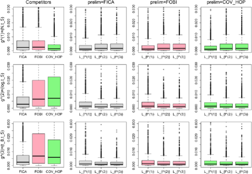
Figure 1: Boxplots of the squared errors $\|\hat{L}-L\|^{2}$ [see (24)] obtained in $M=2\mbox{,}000$ replications from setups $d=1,2,3$ (associated with underlying distributions $g^{(d)}$, $d=1,2,3$) for the competitors $\hat{L}_{\mathrm{FICA}}$, $\hat{L}_{\mathrm{FOBI}}$ and $\hat{L}_{\mathrm{COV}\_\mathrm{HOP}}$, and the nine $R$-estimators $\hat{L}_{f}$ resulting from all combinations of a target density $f^{(j)}=g^{(j)}$, $j=1,2,3$, and one of the three preliminary estimators $\hat{L}_{\mathrm{FICA}}$, $\hat{L}_{\mathrm{FOBI}}$ and $\hat{L}_{\mathrm{COV}\_\mathrm{HOP}}$; see Section 5 for details. The sample size is $n=4\mbox{,}000$.

The results show that, in each setup, all $R$-estimators dramatically improve over their competitors. The behavior of the $R$-estimators does not much depend on the preliminary estimator $\tilde{L}$ used. Optimality of $\hat{L}_{f^{(d)}}$ in Setup $d$ is confirmed. Most importantly, as stated for hypothesis testing at the end of Section 3, the performances of the $R$-estimators do not depend much on the target density $f^{(j)}$ adopted, so that one should not worry much about the choice of the target density in practice. Quite surprisingly, $R$-estimators behave remarkably well even when based on preliminary estimators that, due to heavy tails, fail to be root-$n$ consistent.

In order to investigate small-sample behavior of the estimates, we reran the exact same simulation with sample size $n=800$; in ICA, where most applications involve sample sizes that are not in hundreds, but much larger, this sample size can indeed be considered small. Results are reported in Figure 2. They indicate that, in Setups 2 and 3, $R$-estimators still improve significantly over their competitors, and particularly over $\hat{L}_{\mathrm{FOBI}}$ and $\hat{L}_{\mathrm{COV}\_\mathrm{HOP}}$. In Setup 1, there seem to be no improvement. Compared to results for $n=4\mbox{,}000$, the behavior of one-step $R$-estimators here depends more on the preliminary estimator used. Performances of $R$-estimators again do not depend crucially on the target density, and optimality under correctly specified densities is preserved in most cases.

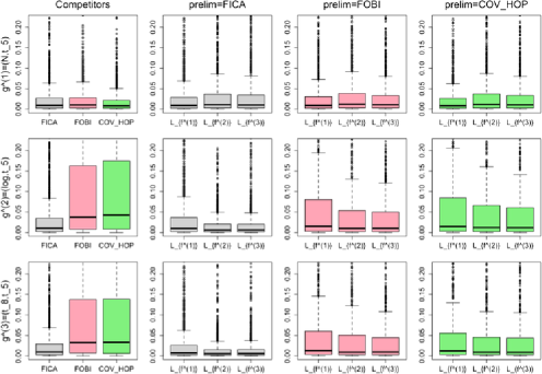
Figure 2: The same boxplots as in Figure 1, but based on sample size $n=800$.

As a conclusion, for practical sample sizes, the proposed $R$-estimators outperform the standard competitors considered, and their behavior is very well in line with our asymptotic results.

Finally, we illustrate the proposed method for estimating cross-information coefficients. We consider again the first 50 replications of our simulation with $n=4\mbox{,}000$, and focus on Setup 1 ($g=g^{(1)}$) and the target density $f=f^{(3)}$ ($\neq$$g^{(1)})$. The cross-information coefficients to be estimated then are $\gamma_{12}(f,g)\approx 1.478$, $\gamma_{21}(f,g)\approx 0.862$, $\rho_{12}(f,g)\approx 1.149$ and $\rho_{21}(f,g)\approx 0.887$. The upper left picture in Figure 3 shows 150 graphs of the mapping $\lambda\mapsto h^{\gamma_{12}}(\lambda)$ (based on $f=f^{(3)}$), among which the 50

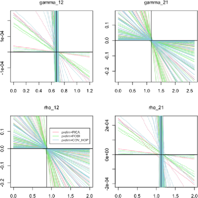
Figure 3: Top left: 150 graphs of the mapping $\lambda\mapsto h^{\gamma_{12}}(\lambda)$ based on $f=f^{(3)}$, associated with the first 50 replications from Setup 1 ($g=g^{(1)}$) in Figure 1 (sample size is $n=4\mbox{,}000$): the 50 curves in pink, green, and blue are based on the preliminary estimators $\hat{L}_{\mathrm{FICA}}$, $\hat{L}_{\mathrm{FOBI}}$ and $\hat{L}_{\mathrm{COV}\_\mathrm{HOP}}$, respectively. Top right, bottom left, and bottom right: the corresponding plots for the mappings $\lambda\mapsto h^{\gamma_{21}}(\lambda)$, $\lambda\mapsto h^{\rho_{12}}(\lambda)$ and $\lambda\mapsto h^{\rho_{21}}(\lambda)$, respectively.

pink curves are based on $\tilde{L}=\hat{L}_{\mathrm{FICA}}$, the 50 green curves are based on $\tilde{L}=\hat{L}_{\mathrm{FOBI}}$, and the 50 blue ones are based on $\tilde{L}=\hat{L}_{\mathrm{COV}\_\mathrm{HOP}}$. The upper right, bottom left and bottom right pictures of the same figure provide the corresponding graphs for the mappings $\lambda\mapsto h^{\gamma_{21}}(\lambda)$, $\lambda\mapsto h^{\rho_{12}}(\lambda)$, and $\lambda\mapsto h^{\rho_{21}}(\lambda)$, respectively. The value at which each graph crosses the $\lambda$-axis is the resulting estimate of the inverse of the associated cross-information coefficient. To be able to evaluate the results, we plotted, in each picture, a vertical black line at the corresponding theoretical value, namely at $1/\gamma_{12}(f,g)$, $1/\gamma_{21}(f,g)$, $1/\rho_{12}(f,g)$ and $1/\rho_{21}(f,g)$. Clearly, the results are excellent, and there does not seem to be much dependence on the preliminary estimator $\tilde{L}$ used.

Appendix A Rank-based efficient central sequences

In this first Appendix, we study the asymptotic behavior of the rank-based efficient central sequences $\underline{\Delta}^{*}_{\vartheta,f;2}$. The main result is the following (see Appendix B for a proof).

Theorem A.1

Fix $\vartheta=(\mu^{\prime},(\operatorname{vecd}^{\circ}L)^{\prime})^{\prime}\in\Theta$ and $f\in\underline{\mathcal{F}}_{\mathrm{ulan}}$. Then, (i) for any $g\in\mathcal{F}$,

$$\underline{\Delta}^{*}_{\vartheta,f;2}=\Delta^{*}_{\vartheta,f,g;2}+o_{L^{2}}(1)$$

as $n\to\infty$, under $\mathrm{P}^{(n)}_{\vartheta,g}$, where $\Delta^{*}_{\vartheta,f,g;2}:=C(I_{p}\otimes L^{-1})^{\prime}\operatorname{vec}[\operatorname{odiag}(\frac{1}{\sqrt{n}}\sum_{i=1}^{n}(S_{i}\odot\varphi_{f}(F_{+}^{-1}(G_{+}(|Z_{i}|))))(S_{i}\odot F_{+}^{-1}(G_{+}(|Z_{i}|)))^{\prime})].$ (ii) Under $\mathrm{P}^{(n)}_{\vartheta+n^{-1/2}\tau,g}$, with $\tau=(\tau_{1}^{\prime},\tau_{2}^{\prime})^{\prime}\in\mathbb{R}^{p}\times\mathbb{R}^{p(p-1)}$ and $g\in{\mathcal{F}}_{\mathrm{ulan}}$,

$$\underline{\Delta}^{*}_{\vartheta,f;2}\stackrel{{\scriptstyle\mathcal{L}}}{{\to}}\mathcal{N}_{p(p-1)}(\Gamma^{*}_{L,f,g;2}\tau_{2},\Gamma^{*}_{L,f;2})$$

as $n\to\infty$ (for $\tau=0$, the result only requires that $g\in\mathcal{F}$). (iii) Still with $\tau=(\tau_{1}^{\prime},\tau_{2}^{\prime})^{\prime}\in\mathbb{R}^{p}\times\mathbb{R}^{p(p-1)}$ and $g\in{\mathcal{F}}_{\mathrm{ulan}}$, $\underline{\Delta}^{*}_{\vartheta+n^{-1/2}\tau,f;2}-\underline{\Delta}_{\vartheta,f;2}^{*}=-\Gamma^{*}_{L,f,g;2}\tau_{2}+o_{\mathrm{P}}(1)$ as $n\to\infty$, under $\mathrm{P}^{(n)}_{\vartheta,g}$.

Both for hypothesis testing and point estimation, we had to replace in $\underline{\Delta}^{*}_{\vartheta,f;2}$ the parameter $\vartheta$ with some estimator ($\check{\vartheta}^{(n)}$, say). The asymptotic behavior of the resulting (so-called aligned) rank-based efficient central sequence $\underline{\Delta}^{*}_{\check{\vartheta}^{(n)},f;2}$ is given in the following result.

Corollary A.1

Fix $\vartheta=(\mu^{\prime},(\operatorname{vecd}^{\circ}L)^{\prime})^{\prime}\in\Theta$, $f\in\underline{\mathcal{F}}_{\mathrm{ulan}}$, and $g\in{\mathcal{F}}_{\mathrm{ulan}}$. Let $\check{\vartheta}=\check{\vartheta}^{(n)}=(\check{\mu}^{\prime},(\operatorname{vecd}^{\circ}\check{L})^{\prime})^{\prime}$ be a locally asymptotically discrete sequence of random vectors satisfying $n^{1/2}(\check{\vartheta}-\vartheta)=O_{\mathrm{P}}(1)$ as $n\to\infty$, under $\mathrm{P}^{(n)}_{\vartheta,g}$. Then $\underline{\Delta}_{\check{\vartheta},f;2}^{*}-\underline{\Delta}_{\vartheta,f;2}^{*}=-\Gamma^{*}_{L,f,g;2}n^{1/2}\operatorname{vecd}^{\circ}(\check{L}-L)+o_{\mathrm{P}}(1),$ still as $n\to\infty$, under $\mathrm{P}^{(n)}_{\vartheta,g}$.

Since the sequence of estimators $\check{\vartheta}^{(n)}$ is assumed to be locally asymptotically discrete [which means that the number of possible values of $\check{\vartheta}^{(n)}$ in balls with $O(n^{-1/2})$ radius centered at $\vartheta$ is bounded as $n\to\infty$], this result is a direct consequence of Theorem A.1(iii) and Lemma 4.4 from kreiss . Local asymptotic discreteness is a concept that goes back to Le Cam and is quite standard in one-step estimation; see, for example, Bi82 or kreiss .

Of course, a sequence of estimators $\check{\vartheta}^{(n)}$ can always be discretized by replacing each component $(\check{\vartheta}^{(n)})_{\ell}$ with

$$\bigl{(}\check{\vartheta}^{(n)}_{\#}\bigr{)}_{\ell}:=(cn^{1/2})^{-1}\operatorname{sign}\bigl{(}\bigl{(}\check{\vartheta}^{(n)}\bigr{)}_{\ell}\bigr{)}\bigl{\lceil}cn^{1/2}\bigl{|}\bigl{(}\check{\vartheta}^{(n)}\bigr{)}_{\ell}\bigr{|}\bigr{\rceil},\qquad\ell=1,\ldots,p^{2},$$

for some arbitrary constant $c>0$. In practice, however, one can safely forget about such discretizations: irrespective of the accuracy of the computer used, the discretization constant $c$ can always be chosen large enough to make discretization be irrelevant at the fixed sample size $n_{0}$ at hand—hence also at any $n>n_{0}$.

Appendix B Proofs

B.1 Proofs of Theorems 2.1 and A.1

The proofs of this section make use of the Hájek projection theorem for linear signed-rank statistics (see, e.g., Pu85 , Chapter 3), which states that, if $Y_{i}=\operatorname{Sign}(Y_{i})|Y_{i}|$, $i=1,\ldots,n$, are i.i.d. with (absolutely continuous) cdf $G$ and if $K\dvtx(0,1)\to\mathbb{R}$ is a continuous and square-integrable score function that can be written as the difference of two monotone increasing functions, then

$$\frac{1}{\sqrt{n}}\sum_{i=1}^{n}\operatorname{Sign}(Y_{i})K(G_{+}(|Y_{i}|))$$ (25)

$$\qquad=\frac{1}{\sqrt{n}}\sum_{i=1}^{n}\operatorname{Sign}(Y_{i})K\biggl{(}\frac{R^{+}_{i}}{n+1}\biggr{)}+o_{L^{2}}(1)$$

$$\qquad=\frac{1}{\sqrt{n}}\sum_{i=1}^{n}\operatorname{Sign}(Y_{i})\mathrm{E}[K(G_{+}(|Y_{i}|))|R^{+}_{i}]+o_{L^{2}}(1)$$ (26)

as $n\to\infty$, where $G_{+}$ stands for the common cdf of the $|Y_{i}|$’s and $R^{+}_{i}$ denotes the rank of $|Y_{i}|$ among $|Y_{1}|,\ldots,|Y_{n}|$. The quantities in (25) and (26) are linear signed-rank quantities that are said to be based on approximate and exact scores, respectively.

In the rest of this section, we fix $\vartheta\in\Theta$, $f\in\underline{\mathcal{F}}_{\mathrm{ulan}}$, and $g\in\mathcal{F}$. We write throughout $Z_{i}$, $S_{i}$, and $R^{+}_{i}$, for $Z_{i}(\vartheta)$, $S_{i}(\vartheta)$, and $R^{+}_{i}(\vartheta)$, respectively. We also write $\mathrm{E}_{h}$ instead of $\mathrm{E}^{(n)}_{\vartheta,h}$, with $h=f,g$. We then start with the proof of Theorem A.1(i). Proof of Theorem A.1(i) Fix $r\neq s\in\{1,\ldots,p\}$ and two score functions $K_{a},K_{b}\dvtx(0,1)\to\mathbb{R}$ with the same properties as $K$ above. Then, by using (i) $\mathrm{E}_{g}[S_{ir}]=0$, (ii) the independence (under $\mathrm{P}^{(n)}_{\vartheta,g}$) between the $S_{ir}$’s and the $(R_{ir},|Z_{ir}|)$’s, and (iii) the independence between the $Z_{ir}$’s and the $Z_{is}$’s, we obtain

$$\mathrm{E}_{g}\Biggl{[}\Biggl{(}\frac{1}{\sqrt{n}}\sum_{i=1}^{n}S_{ir}S_{is}\biggl{(}K_{a}(G_{+r}(|Z_{ir}|))K_{b}(G_{+s}(|Z_{is}|))$$

$$\qquad\quad\hskip 82.2pt{}-K_{a}\biggl{(}\frac{R^{+}_{ir}}{n+1}\biggr{)}K_{b}\biggl{(}\frac{R^{+}_{is}}{n+1}\biggr{)}\biggr{)}\Biggr{)}^{2}\Biggr{]}$$

$$\qquad=\frac{1}{n}\sum_{i=1}^{n}\mathrm{E}_{g}\biggl{[}\biggl{(}K_{a}(G_{+r}(|Z_{ir}|))K_{b}(G_{+s}(|Z_{is}|))$$

$$\qquad\quad\hskip 72.2pt{}-K_{a}\biggl{(}\frac{R^{+}_{ir}}{n+1}\biggr{)}K_{b}\biggl{(}\frac{R^{+}_{is}}{n+1}\biggr{)}\biggr{)}^{2}\biggr{]}$$

$$\qquad\leq 2\mathrm{E}_{g}\biggl{[}\biggl{(}K_{a}(G_{+r}(|Z_{ir}|))-K_{a}\biggl{(}\frac{R^{+}_{ir}}{n+1}\biggr{)}\biggr{)}^{2}\biggr{]}\mathrm{E}_{g}[K^{2}_{b}(G_{+s}(|Z_{is}|))]$$

$$\qquad\quad{}+2\mathrm{E}_{g}\biggl{[}K^{2}_{a}\biggl{(}\frac{R^{+}_{ir}}{n+1}\biggr{)}\biggr{]}\mathrm{E}_{g}\biggl{[}\biggl{(}K_{b}(G_{+s}(|Z_{is}|))-K_{b}\biggl{(}\frac{R^{+}_{is}}{n+1}\biggr{)}\biggr{)}^{2}\biggr{]}.$$

Consequently, the square integrability of $K_{a}$, $K_{b}$, and the convergence to zero of both $\mathrm{E}_{g}[(K_{a}(G_{+r}(|Z_{ir}|))-K_{a}(\frac{R^{+}_{ir}}{n+1}))^{2}]$ and $\mathrm{E}_{g}[(K_{b}(G_{+r}(|Z_{is}|))-K_{b}(\frac{R^{+}_{is}}{n+1}))^{2}]$ [which directly follows from (25)] entail

$$\frac{1}{\sqrt{n}}\sum_{i=1}^{n}S_{ir}S_{is}K_{a}(G_{+r}(|Z_{ir}|))K_{b}(G_{+s}(|Z_{is}|))$$

$$\qquad=\frac{1}{\sqrt{n}}\sum_{i=1}^{n}S_{ir}S_{is}K_{a}\biggl{(}\frac{R^{+}_{ir}}{n+1}\biggr{)}K_{b}\biggl{(}\frac{R^{+}_{is}}{n+1}\biggr{)}+o_{L^{2}}(1)$$

as $n\to\infty$, under $\mathrm{P}^{(n)}_{\vartheta,g}$. Theorem A.1(i) follows by taking $K_{a}=\varphi_{f_{r}}\circ F_{+r}^{-1}$ and $K_{b}=F_{+s}^{-1}$.

We go on with the proof of Theorem 2.1, for which it is important to note that, by proceeding as in the proof of Theorem A.1(i) but with (26) instead of (25), we further obtain that

$$\frac{1}{\sqrt{n}}\sum_{i=1}^{n}S_{ir}S_{is}K_{a}(G_{+r}(|Z_{ir}|))K_{b}(G_{+s}(|Z_{is}|))$$

$$\qquad=\frac{1}{\sqrt{n}}\sum_{i=1}^{n}S_{ir}S_{is}K_{a}\biggl{(}\frac{R^{+}_{ir}}{n+1}\biggr{)}K_{b}\biggl{(}\frac{R^{+}_{is}}{n+1}\biggr{)}+o_{L^{2}}(1)$$

(27)

$$\qquad=\frac{1}{\sqrt{n}}\sum_{i=1}^{n}S_{ir}S_{is}\mathrm{E}_{g}[K_{a}(G_{+r}(|Z_{ir}|))|R_{+{ir}}]$$

$$\qquad\quad\hphantom{\frac{1}{\sqrt{n}}\sum_{i=1}^{n}}{}\times\mathrm{E}_{g}[K_{b}(G_{+s}(|Z_{is}|))|R_{+{is}}]+o_{L^{2}}(1),$$

still as $n\to\infty$ under $\mathrm{P}^{(n)}_{\vartheta,g}$. Proof of Theorem 2.1 It is sufficient to prove Theorem 2.1(i) only, since, as already mentioned at the end of Section 2.3, Theorem 2.1(ii) follows from (8) and Theorem 2.1(i). That is, we have to show that, for any $r,s\in\{1,\ldots,p\}$,

$$\mathrm{E}_{f}\Biggl{[}\frac{1}{\sqrt{n}}\sum_{i=1}^{n}\bigl{(}\varphi_{f}(Z_{i})Z_{i}^{\prime}-I_{p}\bigr{)}_{rs}|S_{1},\ldots,S_{n},R^{+}_{1},\ldots,R^{+}_{n}\Biggr{]}$$

(28)

$$\qquad=(\underline{T}_{\vartheta,f})_{rs}+o_{L^{2}}(1)$$

as $n\to\infty$, under $\mathrm{P}^{(n)}_{\vartheta,f}$. Now, the left-hand side of (B.1) rewrites

$$\mathrm{E}_{f}\Biggl{[}\frac{1}{\sqrt{n}}\sum_{i=1}^{n}\bigl{(}\varphi_{f}(Z_{i})Z_{i}^{\prime}-I_{p}\bigr{)}_{rs}|S_{1},\ldots,S_{n},R^{+}_{1},\ldots,R^{+}_{n}\Biggr{]}$$

$$\qquad=\frac{1}{\sqrt{n}}\sum_{i=1}^{n}\mathrm{E}_{f}[S_{ir}S_{is}\varphi_{f}(|Z_{ir}|)|Z_{is}|-\delta_{rs}|S_{1},\ldots,S_{n},R^{+}_{1},\ldots,R^{+}_{n}]$$

$$\qquad=\frac{1}{\sqrt{n}}\sum_{i=1}^{n}\bigl{(}S_{ir}S_{is}\mathrm{E}_{f}[\varphi_{f}(|Z_{ir}|)|Z_{is}||R^{+}_{1r},\ldots,R^{+}_{nr},R^{+}_{1s},\ldots,R^{+}_{ns}]-\delta_{rs}\bigr{)}.$$

For $r\neq s$, this yields

$$\mathrm{E}_{f}\Biggl{[}\frac{1}{\sqrt{n}}\sum_{i=1}^{n}\bigl{(}\varphi_{f}(Z_{i})Z_{i}^{\prime}-I_{p}\bigr{)}_{rs}|S_{1},\ldots,S_{n},R^{+}_{1},\ldots,R^{+}_{n}\Biggr{]}$$

$$\qquad=\frac{1}{\sqrt{n}}\sum_{i=1}^{n}S_{ir}S_{is}\mathrm{E}_{f}[\varphi_{f}(|Z_{ir}|)|R^{+}_{1r},\ldots,R^{+}_{nr}]\mathrm{E}_{f}[|Z_{is}||R^{+}_{1s},\ldots,R^{+}_{ns}]$$

$$\qquad=\frac{1}{\sqrt{n}}\sum_{i=1}^{n}S_{ir}S_{is}\varphi_{f_{r}}\biggl{(}F_{+r}^{-1}\biggl{(}\frac{R^{+}_{ir}}{n+1}\biggr{)}\biggr{)}F_{+r}^{-1}\biggl{(}\frac{R^{+}_{is}}{n+1}\biggr{)}+o_{L^{2}}(1)$$

$$\qquad=(\underline{T}_{\vartheta,f})_{rs}+o_{L^{2}}(1)$$

as $n\to\infty$, under $\mathrm{P}^{(n)}_{\vartheta,f}$, where we have used (B.1), still with $K_{a}=\varphi_{f_{r}}\circ F_{+r}^{-1}$ and $K_{b}=F_{+s}^{-1}$, but this time at $g=f$. This establishes (B.1) for $r\neq s$. As for $r=s$, (B.1) now entails [writing $K_{ab}(u):=\varphi_{f}(F_{+r}^{-1}(u))\times F_{+r}^{-1}(u)$ for all $u$]

$$\mathrm{E}_{f}\Biggl{[}\frac{1}{\sqrt{n}}\sum_{i=1}^{n}\bigl{(}\varphi_{f}(Z_{i})Z_{i}^{\prime}-I_{p}\bigr{)}_{rs}|S_{1},\ldots,S_{n},R^{+}_{1},\ldots,R^{+}_{n}\Biggr{]}$$

$$\qquad=\Biggl{(}\frac{1}{\sqrt{n}}\sum_{i=1}^{n}\mathrm{E}_{f}[\varphi_{f}(|Z_{ir}|)|Z_{ir}||R^{+}_{1r},\ldots,R^{+}_{nr}]\Biggr{)}-\sqrt{n}$$

$$\qquad=\mathrm{E}_{f}\Biggl{[}\frac{1}{\sqrt{n}}\sum_{i=1}^{n}K_{ab}(F_{+r}(|Z_{ir}|))|R^{+}_{1r},\ldots,R^{+}_{nr}\Biggr{]}-\sqrt{n}$$

$$\qquad=\frac{1}{\sqrt{n}}\sum_{i=1}^{n}K_{ab}\biggl{(}\frac{R^{+}_{i}}{n+1}\biggr{)}-\sqrt{n}+o_{L^{2}}(1)$$ (30)

$$\qquad=\frac{1}{\sqrt{n}}\sum_{i=1}^{n}K_{ab}\biggl{(}\frac{i}{n+1}\biggr{)}-\sqrt{n}+o_{L^{2}}(1)$$

$$\qquad=\sqrt{n}\int_{0}^{1}K_{ab}(u)\,du-\sqrt{n}+o_{L^{2}}(1)$$ (31)

$$\qquad=o_{L^{2}}(1),$$ (32)

still as $n\to\infty$, under $\mathrm{P}^{(n)}_{\vartheta,f}$, where (30), (31) and (32) follow from the Hájek projection theorem for linear rank (not signed-rank) statistics (see, e.g., Pu85 , Chapter 2), the square-integrability of $K_{ab}(\cdot)$ (see the proof of Proposition 3.2(i) in r15 ), and integration by parts, respectively. This further proves (B.1) for $r=s$, hence also the result. Proof of Theorem A.1(ii) and (iii) (ii) In view of Theorem A.1(i), it is sufficient to show that both asymptotic normality results hold for $\Delta^{*}_{\vartheta,f,g;2}$. The result under $\mathrm{P}^{(n)}_{\vartheta,g}$ then straightforwardly follows from the multivariate CLT. As for the result under local alternatives [which, just as the result in part (iii), requires that $g\in\mathcal{F}_{\mathrm{ulan}}$], it is obtained as usual, by establishing the joint normality under $\mathrm{P}^{(n)}_{\vartheta,g}$ of $\log(d\mathrm{P}^{(n)}_{\vartheta+n^{-1/2}\tau,g}/d\mathrm{P}^{(n)}_{\vartheta,g})$ and $\Delta^{*}_{\vartheta,f,g;2}$, then applying Le Cam’s third lemma; the required joint normality follows from a routine application of the classical Cramér–Wold device. (iii) The proof, that is long and tedious, is also a quite trivial adaptation of the proof of Proposition A.1 in Ha06c . We therefore omit it.

B.2 Proof of Theorem 3.1

(i) Applying Corollary A.1, with $\check{\vartheta}:=\break\hat{\vartheta}_{0}=(\hat{\mu}^{\prime},(\operatorname{vecd}^{\circ}L_{0})^{\prime})^{\prime}$ and $\vartheta:=\vartheta_{0}=(\mu^{\prime},(\operatorname{vecd}^{\circ}L_{0})^{\prime})^{\prime}$, entails that $\underline{\Delta}^{*}_{\hat{\vartheta}_{0},f;2}=\underline{\Delta}^{*}_{\vartheta_{0},f;2}+o_{\mathrm{P}}(1)$ as $n\to\infty$ under $\mathrm{P}^{(n)}_{\vartheta_{0},g}$. Consequently, we have that

$$\underline{Q}_{f}=(\operatorname{vec}\underline{\Delta}^{*}_{\vartheta_{0},f;2})^{\prime}(\Gamma^{*}_{L_{0},f;2})^{-1}(\operatorname{vec}\underline{\Delta}^{*}_{\vartheta_{0},f;2})+o_{\mathrm{P}}(1),$$ (33)

still as $n\to\infty$, under $\mathrm{P}^{(n)}_{\vartheta_{0},g}$—hence also under $\mathrm{P}^{(n)}_{\vartheta_{0}+n^{-1/2}\tau,g}$ (from contiguity). The result then follows from Theorem A.1(ii). (ii) It directly follows from (i) that, under the sequence of local alternatives $\mathrm{P}^{(n)}_{\vartheta_{0}+n^{-1/2}\tau,f}$, $\underline{\phi}_{f}^{(n)}$ has asymptotic power $1-\Psi_{p(p-1)}(\chi^{2}_{p(p-1),1-\alpha};\tau_{2}^{\prime}\Gamma^{*}_{L_{0},f;2}\tau_{2})$. This establishes the result, since these local powers coincide with the semiparametrically optimal (at $f$) powers in (7).

B.3 Proofs of Lemma 4.1, Theorems 4.1 and 4.2

Proof of Theorem 4.1 (i) Fix $\vartheta\in\Theta$ and $g\in\mathcal{F}_{\mathrm{ulan}}$. From (15), the fact that $\hat{\Gamma}^{*}_{\tilde{L},f;2}-\Gamma^{*}_{L,f,g;2}=o_{\mathrm{P}}(1)$ as $n\to\infty$ under $\mathrm{P}^{(n)}_{\vartheta,g}$, and Corollary A.1, we obtain

$$\quad\sqrt{n}\operatorname{vecd}^{\circ}(\hat{\underline{L}}_{f}-L) = \sqrt{n}\operatorname{vecd}^{\circ}(\tilde{L}-L)+(\hat{\Gamma}^{*}_{\tilde{L},f;2})^{-1}\underline{\Delta}^{*}_{\tilde{\vartheta},f;2}$$ (34)

$$= \sqrt{n}\operatorname{vecd}^{\circ}(\tilde{L}-L)+(\Gamma^{*}_{L,f,g;2})^{-1}\underline{\Delta}^{*}_{\tilde{\vartheta},f;2}+o_{\mathrm{P}}(1)$$

$$= (\Gamma^{*}_{L,f,g;2})^{-1}\underline{\Delta}^{*}_{\vartheta,f;2}+o_{\mathrm{P}}(1)$$

as $n\to\infty$ under $\mathrm{P}^{(n)}_{\vartheta,g}$. Consequently, Theorem A.1(i) and (ii) entails that, still as $n\to\infty$ under $\mathrm{P}^{(n)}_{\vartheta,g}$,

$$\sqrt{n}\operatorname{vecd}^{\circ}(\hat{\underline{L}}_{f}-L)$$

(35)

$$\qquad=(\Gamma^{*}_{L,f,g;2})^{-1}{\Delta}^{*}_{\vartheta,f,g;2}+o_{\mathrm{P}}(1)$$

$$\qquad\stackrel{{\scriptstyle\mathcal{L}}}{{\to}}\mathcal{N}_{p(p-1)}(0,(\Gamma^{*}_{L,f,g;2})^{-1}\Gamma^{*}_{L,f;2}(\Gamma^{*}_{L,f,g;2})^{-1\prime}).$$ (36)

Now, by using the fact that $C^{\prime}(\operatorname{vecd}^{\circ}H)=(\operatorname{vec}H)$ for any $p\times p$ matrix $H$ with only zero diagonal entries, we have that $\sqrt{n}\operatorname{vec}(\hat{\underline{L}}_{f}-L)=\sqrt{n}C^{\prime}\operatorname{vecd}^{\circ}(\hat{\underline{L}}_{f}-L)$, so that (16), (17) and (18) follow from (34), (B.3) and (36), respectively.

(ii) The asymptotic covariance matrix of $\sqrt{n}\operatorname{vecd}^{\circ}(\hat{\underline{L}}_{f}-L)$, under $\mathrm{P}^{(n)}_{\vartheta,f}$, reduces to $(\Gamma^{*}_{L,f;2})^{-1}$ [let $g=f$ in (36)], which establishes the result.

To prove Theorem 4.2, we will need the following result.

Lemma B.1

Fix $\vartheta=(\mu^{\prime},(\operatorname{vecd}^{\circ}L)^{\prime})^{\prime}\in\Theta$ and $f,g\in\mathcal{F}_{\mathrm{ulan}}$. Then

$$(I_{p}\otimes L^{-1})C^{\prime}(\Gamma^{*}_{L,f,g;2})^{-1}C(I_{p}\otimes L^{-1})^{\prime}$$

$$\qquad=\sum_{r,s=1,r\neq s}^{p}\bigl{\{}\alpha_{rs}(f,g)\bigl{(}e_{r}e_{r}^{\prime}\otimes(L_{rs}^{2}e_{r}e_{r}^{\prime}+e_{s}e_{s}^{\prime}-L_{rs}e_{r}e_{s}^{\prime}-L_{rs}e_{s}e_{r}^{\prime})\bigr{)}$$

$$\hphantom{\sum_{r,s=1,r\neq s}^{p}\bigl{\{}}\qquad\quad{}+\beta_{rs}(f,g)\bigl{(}e_{r}e_{s}^{\prime}\otimes(L_{rs}L_{sr}e_{r}e_{s}^{\prime}-L_{rs}e_{r}e_{r}^{\prime}-L_{sr}e_{s}e_{s}^{\prime}+e_{s}e_{r}^{\prime})\bigr{)}\bigr{\}},$$

where $L_{rs}$ denotes the entry $(r,s)$ of $L$.

Proof of Theorem 4.2 By using again the fact that $C^{\prime}(\operatorname{vecd}^{\circ}H)=(\operatorname{vec}H)$ for any $p\times p$ matrix $H$ with only zero diagonal entries, and then Lemma B.1, we obtain

$$\operatorname{vec}(\hat{\underline{L}}_{f}-\tilde{L})$$

$$\qquad=C^{\prime}\operatorname{vecd}^{\circ}(\hat{\underline{L}}_{f}-\tilde{L})$$

$$\qquad=\frac{1}{\sqrt{n}}C^{\prime}(\hat{\Gamma}^{*}_{\tilde{L},f;2})^{-1}C(I_{p}\otimes\tilde{L}^{-1})^{\prime}\operatorname{vec}\underline{T}_{\tilde{\vartheta},f}$$

$$\qquad=\frac{1}{\sqrt{n}}(I_{p}\otimes\tilde{L})$$

$$\qquad\quad{}\times\Biggl{[}\sum_{r,s=1,r\neq s}^{p}\bigl{\{}\hat{\alpha}_{rs}(f)\bigl{(}e_{r}e_{r}^{\prime}\otimes(\tilde{L}_{rs}^{2}e_{r}e_{r}^{\prime}+e_{s}e_{s}^{\prime}-\tilde{L}_{rs}e_{r}e_{s}^{\prime}-\tilde{L}_{rs}e_{s}e_{r}^{\prime})\bigr{)}$$

$$\hskip 59.0pt\qquad\quad{}+\hat{\beta}_{rs}(f)\bigl{(}e_{r}e_{s}^{\prime}\otimes(\tilde{L}_{rs}\tilde{L}_{sr}e_{r}e_{s}^{\prime}-\tilde{L}_{rs}e_{r}e_{r}^{\prime}$$

$$\qquad\quad\hskip 210.0pt{}-\tilde{L}_{sr}e_{s}e_{s}^{\prime}+e_{s}e_{r}^{\prime})\bigr{)}\bigr{\}}\Biggr{]}$$

$$\qquad\quad{}\times\operatorname{vec}\underline{T}_{\tilde{\vartheta},f}.$$

Since all diagonal entries of $\underline{T}_{\tilde{\vartheta},f}$ are zeros, we have that

$$\operatorname{vec}(\hat{\underline{L}}_{f}-\tilde{L})$$

$$\qquad=\frac{1}{\sqrt{n}}(I_{p}\otimes\tilde{L})$$

$$\qquad\quad{}\times\Biggl{[}\sum_{r,s=1,r\neq s}^{p}\bigl{\{}\hat{\alpha}_{rs}(f)\bigl{(}e_{r}e_{r}^{\prime}\otimes(e_{s}e_{s}^{\prime}-\tilde{L}_{rs}e_{r}e_{s}^{\prime})\bigr{)}$$

$$\hskip 59.3pt\qquad\quad{}+\hat{\beta}_{rs}(f)\bigl{(}e_{r}e_{s}^{\prime}\otimes(e_{s}e_{r}^{\prime}-\tilde{L}_{rs}e_{r}e_{r}^{\prime})\bigr{)}\bigr{\}}\Biggr{]}\operatorname{vec}\underline{T}_{\tilde{\vartheta},f}.$$

The identity $(C^{\prime}\otimes A)(\operatorname{vec}B)=\operatorname{vec}(ABC)$ then yields

$$\operatorname{vec}(\hat{\underline{L}}_{f}-\tilde{L})=\frac{1}{\sqrt{n}}(I_{p}\otimes\tilde{L})\operatorname{vec}\Biggl{[}\sum_{r,s=1,r\neq s}^{p}(\hat{N}_{f})_{sr}(e_{s}e_{r}^{\prime}-\tilde{L}_{rs}e_{r}e_{r}^{\prime})\Biggr{]}.$$

Hence, we have

$$\hat{\underline{L}}_{f}-\tilde{L} = \frac{1}{\sqrt{n}}\tilde{L}\sum_{r,s=1,r\neq s}^{p}(\hat{N}_{f})_{sr}(e_{s}e_{r}^{\prime}-\tilde{L}_{rs}e_{r}e_{r}^{\prime})$$

$$= \frac{1}{\sqrt{n}}\tilde{L}\sum_{r,s=1}^{p}(\hat{N}_{f})_{sr}(e_{s}e_{r}^{\prime}-\tilde{L}_{rs}e_{r}e_{r}^{\prime})$$

$$= \frac{1}{\sqrt{n}}\tilde{L}\Biggl{(}N_{f}-\sum_{r,s=1}^{p}\tilde{L}_{rs}(\hat{N}_{f})_{sr}e_{r}e_{r}^{\prime}\Biggr{)}$$

$$= \frac{1}{\sqrt{n}}\tilde{L}\Biggl{(}\hat{N}_{f}-\sum_{r=1}^{p}(\tilde{L}N_{f})_{rr}e_{r}e_{r}^{\prime}\Biggr{)}$$

$$= \frac{1}{\sqrt{n}}\tilde{L}\bigl{(}\hat{N}_{f}-\operatorname{diag}(\tilde{L}N_{f})\bigr{)},$$

which proves the result. Proof of Lemma 4.1 In this proof, all stochastic convergences are as $n\to\infty$ under $\mathrm{P}^{(n)}_{\vartheta,g}$. First note that, if $\check{\vartheta}:=(\check{\mu}^{\prime},(\operatorname{vecd}^{\circ}\check{L})^{\prime})^{\prime}$ is an arbitrary locally asymptotically discrete root-$n$ consistent estimator for $\vartheta=(\mu^{\prime},(\operatorname{vecd}^{\circ}L)^{\prime})^{\prime}$, we then have that

$$\operatorname{vec}(\underline{T}_{\check{\vartheta},f}-\underline{T}_{\vartheta,f}) = -G_{f,g}(I_{p}\otimes\check{L}^{-1})C^{\prime}\sqrt{n}\operatorname{vecd}^{\circ}(\check{L}-L)$$

$${}+o_{\mathrm{P}}(1)$$

(compare with Corollary A.1). Incidentally, note that (B.3) implies that $\operatorname{vec}\underline{T}_{\check{\vartheta},f}$ is $O_{\mathrm{P}}(1)$ [by proceeding exactly as in the proof of Theorem A.1(i) and (ii), we can indeed show that, under $\mathrm{P}^{(n)}_{\vartheta,g}$, $\operatorname{vec}\underline{T}_{\vartheta,f}$ is asymptotically multinormal, hence stochastically bounded].

Now, from (B.3), we obtain

$$\operatorname{vec}(\underline{T}_{\tilde{\vartheta}_{\lambda}^{\gamma_{rs}},f}-\underline{T}_{\tilde{\vartheta},f})$$

$$\qquad=-G_{f,g}(I_{p}\otimes\tilde{L}^{-1})C^{\prime}\sqrt{n}\operatorname{vecd}^{\circ}(\tilde{L}_{\lambda}^{\gamma_{rs}}-\tilde{L})+o_{\mathrm{P}}(1)$$

$$\qquad=-\lambda(\underline{T}_{\tilde{\vartheta},f})_{rs}G_{f,g}(I_{p}\otimes\tilde{L}^{-1})C^{\prime}\operatorname{vecd}^{\circ}\bigl{(}\tilde{L}e_{r}e_{s}^{\prime}-\tilde{L}\operatorname{diag}(\tilde{L}e_{r}e_{s}^{\prime})\bigr{)}+o_{\mathrm{P}}(1),$$

which, by using the fact that $C^{\prime}(\operatorname{vecd}^{\circ}H)=(\operatorname{vec}H)$ for any $p\times p$ matrix $H$ with only zero diagonal entries, leads to

$$\operatorname{vec}(\underline{T}_{\tilde{\vartheta}_{\lambda}^{\gamma_{rs}},f}-\underline{T}_{\tilde{\vartheta},f})$$

$$\qquad=-\lambda(\underline{T}_{\tilde{\vartheta},f})_{rs}G_{f,g}(I_{p}\otimes\tilde{L}^{-1})\operatorname{vec}\bigl{(}\tilde{L}e_{r}e_{s}^{\prime}-\tilde{L}\operatorname{diag}(\tilde{L}e_{r}e_{s}^{\prime})\bigr{)}+o_{\mathrm{P}}(1)$$

$$\qquad=-\lambda(\underline{T}_{\tilde{\vartheta},f})_{rs}G_{f,g}\operatorname{vec}\bigl{(}e_{r}e_{s}^{\prime}-\operatorname{diag}(\tilde{L}e_{r}e_{s}^{\prime})\bigr{)}+o_{\mathrm{P}}(1).$$

This yields

$$\operatorname{vec}(\underline{T}_{\tilde{\vartheta}_{\lambda}^{\gamma_{rs}},f}-\underline{T}_{\tilde{\vartheta},f})$$

$$\qquad=-\lambda(\underline{T}_{\tilde{\vartheta},f})_{rs}G_{f,g}\operatorname{vec}(e_{r}e_{s}^{\prime})+o_{\mathrm{P}}(1)$$

$$\qquad=-\lambda(\underline{T}_{\tilde{\vartheta},f})_{rs}\bigl{(}\gamma_{rs}(f,g)\operatorname{vec}(e_{r}e_{s}^{\prime})+\rho_{rs}(f,g)\operatorname{vec}(e_{s}e_{r}^{\prime})\bigr{)}$$

$$\qquad\quad{}+o_{\mathrm{P}}(1).$$

Premultiplying by $(\underline{T}_{\tilde{\vartheta},f})_{rs}(e_{s}\otimes e_{r})^{\prime}$, we then obtain

$$(\underline{T}_{\tilde{\vartheta},f})_{rs}(\underline{T}_{\tilde{\vartheta}_{\lambda}^{\gamma_{rs}},f})_{rs}-((\underline{T}_{\tilde{\vartheta},f})_{rs})^{2}=-\lambda((\underline{T}_{\tilde{\vartheta},f})_{rs})^{2}\gamma_{rs}(f,g)+o_{\mathrm{P}}(1)$$

[recall indeed that $\underline{T}_{\tilde{\vartheta},f}=O_{\mathrm{P}}(1)$], which establishes the $\gamma$-part of the lemma. The proof of the $\rho$-part follows along the exact same lines, but for the fact that the premultiplication is by $(\underline{T}_{\tilde{\vartheta},f})_{sr}(e_{r}\otimes e_{s})^{\prime}$.

References

- (1) {barticle}[auto:STB—2011/09/12—07:03:23] \bauthor\bsnmAmari, \bfnmS.\binitsS. (\byear2002). \btitleIndependent component analysis and method of estimating functions. \bjournalIEICE Trans. Fundamentals Electronics, Communications and Computer Sciences \bvolumeE85-A \bpages540–547. \bptokimsref \endbibitem
- (2) {barticle}[mr] \bauthor\bsnmBickel, \bfnmP. J.\binitsP. J. (\byear1982). \btitleOn adaptive estimation. \bjournalAnn. Statist. \bvolume10 \bpages647–671. \bidissn=0090-5364, mr=0663424 \bptokimsref \endbibitem
- (3) {bbook}[auto:STB—2011/09/12—07:03:23] \bauthor\bsnmBickel, \bfnmP. J.\binitsP. J., \bauthor\bsnmKlaassen, \bfnmC. A. J.\binitsC. A. J., \bauthor\bsnmRitov, \bfnmY.\binitsY. and \bauthor\bsnmWellner, \bfnmJ. A.\binitsJ. A. (\byear1993). \btitleEfficient and Adaptive Statistical Inference for Semiparametric Models. \bpublisherJohns Hopkins Univ. Press, \baddressBaltimore. \bptokimsref \endbibitem
- (4) {bmisc}[auto:STB—2011/09/12—07:03:23] \bauthor\bsnmCardoso, \bfnmJ. F.\binitsJ. F. (\byear1989). \bhowpublishedSource separation using higher moments. In Proceedings of IEEE International Conference on Acoustics, Speech and Signal Processing, Glasgow 2109–2112. \bptokimsref \endbibitem
- (5) {bincollection}[auto:STB—2011/09/12—07:03:23] \bauthor\bsnmCassart, \bfnmD.\binitsD., \bauthor\bsnmHallin, \bfnmM.\binitsM. and \bauthor\bsnmPaindaveine, \bfnmD.\binitsD. (\byear2010). \btitleOn the estimation of cross-information quantities in R-estimation. In \bbooktitleNonparametrics and Robustness in Modern Statistical Inference and Time Series Analysis: A Festschrift in Honor of Professor Jana Jurečková (\beditor\bfnmJ.\binitsJ. \bsnmAntoch, \beditor\bfnmM.\binitsM. \bsnmHušková and \beditor\bfnmP. K.\binitsP. K. \bsnmSen, eds.) \bpages35–45. \bpublisherIMS, \baddressBeachwood, OH. \bptokimsref \endbibitem
- (6) {barticle}[mr] \bauthor\bsnmChen, \bfnmAiyou\binitsA. and \bauthor\bsnmBickel, \bfnmPeter J.\binitsP. J. (\byear2006). \btitleEfficient independent component analysis. \bjournalAnn. Statist. \bvolume34 \bpages2825–2855. \biddoi=10.1214/009053606000000939, issn=0090-5364, mr=2329469 \bptokimsref \endbibitem
- (7) {barticle}[mr] \bauthor\bsnmHallin, \bfnmMarc\binitsM., \bauthor\bsnmOja, \bfnmHannu\binitsH. and \bauthor\bsnmPaindaveine, \bfnmDavy\binitsD. (\byear2006). \btitleSemiparametrically efficient rank-based inference for shape. II. Optimal -estimation of shape. \bjournalAnn. Statist. \bvolume34 \bpages2757–2789. \biddoi=10.1214/009053606000000948, issn=0090-5364, mr=2329466 \bptokimsref \endbibitem
- (8) {barticle}[mr] \bauthor\bsnmHallin, \bfnmMarc\binitsM. and \bauthor\bsnmPaindaveine, \bfnmDavy\binitsD. (\byear2006). \btitleSemiparametrically efficient rank-based inference for shape. I. Optimal rank-based tests for sphericity. \bjournalAnn. Statist. \bvolume34 \bpages2707–2756. \biddoi=10.1214/009053606000000731, issn=0090-5364, mr=2329465 \bptokimsref \endbibitem
- (9) {bmisc}[auto:STB—2011/09/12—07:03:23] \bauthor\bsnmHallin, \bfnmM.\binitsM. and \bauthor\bsnmPaindaveine, \bfnmD.\binitsD. (\byear2008). \bhowpublishedSemiparametrically efficient one-step R-estimation. Unpublished manuscript. Univ. Libre de Bruxelles. \bptokimsref \endbibitem
- (10) {barticle}[mr] \bauthor\bsnmHallin, \bfnmMarc\binitsM., \bauthor\bsnmVermandele, \bfnmCatherine\binitsC. and \bauthor\bsnmWerker, \bfnmBas\binitsB. (\byear2006). \btitleSerial and nonserial sign-and-rank statistics: Asymptotic representation and asymptotic normality. \bjournalAnn. Statist. \bvolume34 \bpages254–289. \biddoi=10.1214/009053605000000769, issn=0090-5364, mr=2275242 \bptokimsref \endbibitem
- (11) {barticle}[mr] \bauthor\bsnmHallin, \bfnmMarc\binitsM. and \bauthor\bsnmWerker, \bfnmBas J. M.\binitsB. J. M. (\byear2003). \btitleSemi-parametric efficiency, distribution-freeness and invariance. \bjournalBernoulli \bvolume9 \bpages137–165. \biddoi=10.3150/bj/1068129013, issn=1350-7265, mr=1963675 \bptokimsref \endbibitem
- (12) {barticle}[auto:STB—2011/09/12—07:03:23] \bauthor\bsnmHyvärinen, \bfnmA.\binitsA. (\byear1999). \btitleFast and robust fixed-point algorithms for independent component analysis. \bjournalIEEE Trans. Neural Networks \bvolume10 \bpages626–634. \bptokimsref \endbibitem
- (13) {barticle}[auto:STB—2011/09/12—07:03:23] \bauthor\bsnmHyvärinen, \bfnmA.\binitsA. and \bauthor\bsnmOja, \bfnmE.\binitsE. (\byear1997). \btitleA fast fixed-point algorithm for independent component analysis. \bjournalNeural Comput. \bvolume9 \bpages1483–1492. \bptokimsref \endbibitem
- (14) {barticle}[mr] \bauthor\bsnmIlmonen, \bfnmPauliina\binitsP., \bauthor\bsnmNevalainen, \bfnmJaakko\binitsJ. and \bauthor\bsnmOja, \bfnmHannu\binitsH. (\byear2010). \btitleCharacteristics of multivariate distributions and the invariant coordinate system. \bjournalStatist. Probab. Lett. \bvolume80 \bpages1844–1853. \biddoi=10.1016/j.spl.2010.08.010, issn=0167-7152, mr=2734250 \bptokimsref \endbibitem
- (15) {bmisc}[auto:STB—2011/09/12—07:03:23] \bauthor\bsnmIlmonen, \bfnmP.\binitsP., \bauthor\bsnmNordhausen, \bfnmK.\binitsK., \bauthor\bsnmOja, \bfnmH.\binitsH. and \bauthor\bsnmOllila, \bfnmE.\binitsE. (\byear2011). \bhowpublishedIndependent component (IC) functionals and a new performance index. Unpublished manuscript. Univ. Tampere. \bptokimsref \endbibitem
- (16) {bmisc}[auto:STB—2011/09/12—07:03:23] \bauthor\bsnmIlmonen, \bfnmP.\binitsP. and \bauthor\bsnmPaindaveine, \bfnmD.\binitsD. (\byear2011). \bhowpublishedSupplement to “Semiparametrically efficient inference based on signed ranks in symmetric independent component models.” DOI:10.1214/11-AOS906SUPP. \bptokimsref \endbibitem
- (17) {barticle}[mr] \bauthor\bsnmKreiss, \bfnmJens-Peter\binitsJ.-P. (\byear1987). \btitleOn adaptive estimation in stationary ARMA processes. \bjournalAnn. Statist. \bvolume15 \bpages112–133. \biddoi=10.1214/aos/1176350256, issn=0090-5364, mr=0885727 \bptokimsref \endbibitem
- (18) {bbook}[mr] \bauthor\bsnmLe Cam, \bfnmLucien\binitsL. (\byear1986). \btitleAsymptotic Methods in Statistical Decision Theory. \bpublisherSpringer, \baddressNew York. \bidmr=0856411 \bptokimsref \endbibitem
- (19) {bmisc}[auto:STB—2011/09/12—07:03:23] \bauthor\bsnmOja, \bfnmH.\binitsH., \bauthor\bsnmPaindaveine, \bfnmD.\binitsD. and \bauthor\bsnmTaskinen, \bfnmS.\binitsS. (\byear2011). \bhowpublishedParametric and nonparametric tests for multivariate independence in IC models. Unpublished manuscript. Univ. Libre de Bruxelles. \bptokimsref \endbibitem
- (20) {barticle}[auto:STB—2011/09/12—07:03:23] \bauthor\bsnmOja, \bfnmH.\binitsH., \bauthor\bsnmSirkiä, \bfnmS.\binitsS. and \bauthor\bsnmEriksson, \bfnmJ.\binitsJ. (\byear2006). \btitleScatter matrices and independent component analysis. \bjournalAustrian J. Statist. \bvolume35 \bpages175–189. \bptokimsref \endbibitem
- (21) {barticle}[mr] \bauthor\bsnmOllila, \bfnmEsa\binitsE. (\byear2010). \btitleThe deflation-based FastICA estimator: Statistical analysis revisited. \bjournalIEEE Trans. Signal Process. \bvolume58 \bpages1527–1541. \biddoi=10.1109/TSP.2009.2036072, issn=1053-587X, mr=2758026 \bptokimsref \endbibitem
- (22) {bmisc}[auto:STB—2011/09/12—07:03:23] \bauthor\bsnmOllila, \bfnmE.\binitsE. and \bauthor\bsnmKim, \bfnmH. J.\binitsH. J. (\byear2011). \bhowpublishedOn testing hypotheses of mixing vectors in the ICA model using FastICA. In Proceedings of IEEE International Symposium on Biomedical Imaging (ISBI’), Chicago, IL 11 325–328. \bptokimsref \endbibitem
- (23) {bbook}[mr] \bauthor\bsnmPuri, \bfnmMadan Lal\binitsM. L. and \bauthor\bsnmSen, \bfnmPranab Kumar\binitsP. K. (\byear1985). \btitleNonparametric Methods in General Linear Models. \bpublisherWiley, \baddressNew York. \bidmr=0794309 \bptokimsref \endbibitem
- (24) {bbook}[mr] \bauthor\bsnmRao, \bfnmC. Radhakrishna\binitsC. R. and \bauthor\bsnmMitra, \bfnmSujit Kumar\binitsS. K. (\byear1971). \btitleGeneralized Inverse of Matrices and Its Applications. \bpublisherWiley, \baddressNew York. \bidmr=0338013 \bptokimsref \endbibitem
- (25) {barticle}[pbm] \bauthor\bsnmTheis, \bfnmFabian J.\binitsF. J. (\byear2004). \btitleA new concept for separability problems in blind source separation. \bjournalNeural Comput. \bvolume16 \bpages1827–1850. \biddoi=10.1162/0899766041336404, issn=0899-7667, pmid=15265324 \bptokimsref \endbibitem